Condition prediction and estimation of service life in the presence of data censoring and dependent competing risks

Abstract

An accurate estimation of service life is of primary interest in pavement management systems limiting the time frame for maintenance and rehabilitation (M&R) treatments. Common condition prediction models are derived by regression analysis at the road network level based on empirical data from periodic condition surveys. If a particular section has not failed prior to the last survey or the condition has improved (e.g. due to treatment), it is considered as censored. If censoring is neglected the performance functions, service lives and estimated costs may show substantial bias. The authors who acknowledge this problem have used standard statistical (survival analysis) techniques accounting for censoring. However, any road section may fail due to different but dependent competing failure causes (risks), each leading to treatments. This constitutes a special type of censoring that cannot be addressed with traditional survival analysis methods relying on the assumption of independent censoring. As the number of failure causes usually exceeds one (e.g. fatigue, permanent deformation, thermal cracking), this case is quite common. Moreover, the time until a first failure depends on the sign and degree of correlation between present failure types being modelled by the overall survival function. This paper presents a critical review and comparison of common regression, Markov chain and survival analysis models with and without correlated competing risks based on computer-generated data. Using performance history and distress progression models at the section level in combination with survival analysis improves the accuracy of predictions in comparison. Furthermore, the paper proposes a simultaneous modelling of joint and marginal service life distributions based on copula functions as generalised solution accounting for dependence between competing risks. As the focus of this paper is on condition prediction with censored data, the distress-specific planning and optimisation of treatments will be covered in forthcoming papers.

Keywords:

• Pavement management
• survival analysis
• dependent competing risks
• data censoring
• service life

1. Introduction

1.1. Data censoring in pavement management

Performance models predict when, where and how (cause of failure) a pavement section will fail (deterministic) or may fail including uncertainties (probabilistic). In addition, performance models may be based on material behaviour and pavement response (mechanistic) or survey data and statistical methods (empirical), or a combination of both (empirical-mechanistic). Currently, mainly pure empirical or empirical-mechanistic (E-M) models are applied for prediction in pavement management at the network level (Schram and Abdelrahman 2009, Kargah-Ostadi and Stoffels 2015). However, due to technical, economical and practical reasons, it is not possible to continuously observe the condition deterioration for all road sections during the entire service life. On the contrary, in most cases only data from two consecutive surveys is available. Moreover, survey methods change over time due to technological advancements and maintenance history is not always properly documented, especially for regional and local roads. Thus, the available data for an estimation of service life and development of performance models is censored. If this property of the empirical survey data is neglected, the estimated service life will be over- or underestimated depending on the type of censoring.

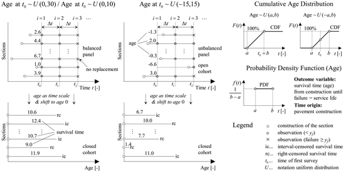
In this paper failure is defined as exceeding a given condition threshold triggering the application of maintenance and rehabilitation treatments. In general, condition thresholds differ among countries, agencies and road classes and have been set more or less arbitrarily (Hoffmann and Donev 2016). Figure 1 provides an overview of all common types of censoring in pavement management. If a road section has failed prior to a first survey, it is considered left censored, i.e. the true (latent) service life is less than the observed service life. Interval censoring occurs if the true lifetime is within a known interval of time (e.g. the survey interval Δt). If a pavement has not failed by the time of the last survey, it is considered right censored, i.e. the observed service life is less than the true service life.

Figure 1. Common types of censoring of the lifetime (service life) of pavements in the context of continuous condition deterioration, application of treatments and periodic condition surveys.

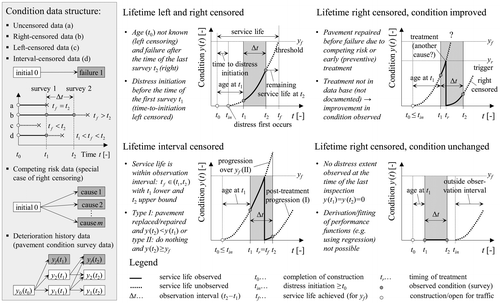
In addition, there are a few special features of condition survey data that have to be considered as well. First, the pavement condition deteriorates continuously reaching different intermediate states before failure in contrast to typical failure-time data with only two discrete states (failure and non-failure). Thus, a model that incorporates this section-specific degradation history will always be superior to other models. Second, a flexible pavement may fail due to one or more failure causes/mechanisms (e.g. rutting, fatigue, low temperature) and a service life can be computed with respect to each failure type as well as an overall service life (time until failure of any cause). Thus, a pavement may be repaired before reaching the end of its service life due to a competing risk failure or due to an early preventive treatment. In this case the failure event cannot be observed in future condition surveys. Finally, for a network with high maintenance standards (highways) the majority of the sections will be in good condition exhibiting no signs of distress. For this case considering only failing sections in the analysis will lead to an underestimation of service life and an overestimation of investment needs. In summary, the provided examples of data censoring are quite common and have to be addressed with appropriate statistical methods.

The reminder of this paper is organised as follows. Sections 1.2 and 1.3 provide an overview of the common survival analysis methods and some applications of these methods in pavement condition data analysis. In Section 2.1, the reasons for using a simulation approach and key settings are explained. In Sections 2.2 to 3.3, the deviations resulting from the application of standard approaches (regression, Markov chains, SA) to the generated data are presented and analysed. Sections 3.4 and 3.5 present innovative ways to overcome the described drawbacks of common models leading to an improved estimation of true service lives. The conclusions regarding comparative analysis and practical application are presented in Section 4.

1.2. Common survival analysis models

Survival analysis (biostatistics), failure-time analysis (engineering), event-history analysis (sociology) or duration analysis (econometrics) provide statistical techniques to estimate the expected time until the occurrence of an event. This event may be an initiation of a distress or failure of a pavement section exceeding a specified condition threshold for a given type of distress. The survival function of a section regarding such an event gives the probability of surviving until time t, while the hazard function gives the instantaneous potential for failure, given survival up to time t (Figure 2(a)). The relationship between survival function S(t), probability density f(t) and hazard function h(t) is of fundamental importance in survival analysis (Kalbfleisch and Prentice 2002, Crowder 2012, Kleinbaum and Klein 2012).

Figure 2. Relationship between probability density, hazard and survival function (a). Parametric likelihood estimation accommodating uncensored, left-, interval- and right-censored data (b).

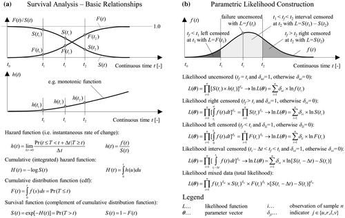
The construction of the parametric likelihood as illustrated in Figure 2(b) is a necessary foundation for understanding the mathematics of survival analysis and correct interpretation of results. The likelihood function L is a function of the observed data, unknown parameters and the probability density of the assumed lifetime distribution. For right-censored observations with failure occurring after the time of observation t, the likelihood contribution is given by the survival function S(t). Left-censored observations (already failed sections) are included in L using the cumulative distribution function F(t). For interval-censored data the likelihood is the difference between survival function estimated at the beginning and the end of the interval. The total likelihood is calculated as a product of n individual likelihood contributions assuming independence between different contributions, i.e. independence between the lifetimes or censoring times of the individual sections. The maximum likelihood estimation method maximises the total likelihood defined as the joint probability of obtaining the observed data with respect to the set of parameters.

Figure 3 provides an overview of common survival-analysis approaches including examples based on Kleinbaum and Klein (2012). The non-parametric Kaplan–Meier (KM) product-limit estimator is based on conditional probability and makes no assumptions about the form of the lifetime distribution. As with other survival-analysis models the validity of the estimation relies on the assumption that the censoring mechanism is statistically independent of the failure process (independent censoring assumption). As attractive as a nonparametric approach might seem, the Kaplan–Meier method cannot accommodate left- and interval-censored data. Out-of-sample prediction or estimation of survival probability beyond the last failure time is also not possible. As a further disadvantage, the model can only account for time-constant categorical explanatory variables (e.g. climatic zone freeze/non-freeze) by stratifying the data and separate analysis.

Figure 3. Overview of classic non-parametric, semi-parametric and parametric models in survival analysis together with their characteristics and limitations.

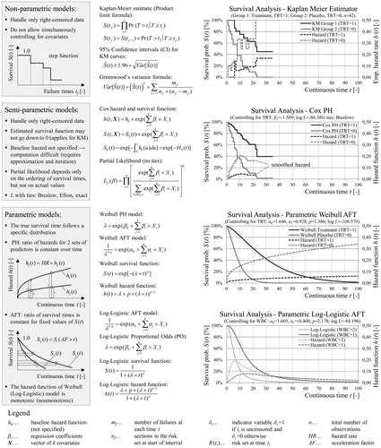
Another popular method is the semi-parametric Cox proportional hazard (PH) model allowing for simultaneous control of covariates without specifying the baseline hazard function. Continuous time-independent variables and interaction terms (product of variables) may be used as explanatory variables. The proportional hazard assumption states that a covariate has a multiplicative effect on the hazard rate that is constant over time. In other words, the ratio of the hazard functions for two different sets of explanatory variables (hazard ratio, HR) does not depend on the time. A time-dependent predictor variable may be accommodated by the extended Cox model that no longer fulfils the PH assumption. Apart from the inclusion of covariates, the Cox model exhibits the same limitations as the KM method. If no covariates are used, as in this paper, the Cox model reduces to the baseline survival function S ₀ (t), which is identical to the KM estimate. For this reason, semi-parametric models are not analysed any further.

In parametric survival analysis the survival and the hazard are fully specified smooth functions being convenient for subsequent optimisation and simulation. Non-parametric estimates, laboratory tests or theoretical assumptions may deliver insights about the selection of an appropriate model form with the exponential, Weibull and log-logistic distributions being very common. Parametric models account for left-, interval- and right-censoring providing even out-of-sample estimates beyond the last failure time. The survival time may be modelled as a function of explanatory variables based on underlying proportionality assumptions (e.g. proportional hazards, accelerated failure time or proportional odds). Parametric models may also incorporate a frailty component to account for unobserved heterogeneity among pavement sections (Kleinbaum and Klein 2012).

In PMS survival analysis may be used as an alternative or better in addition to regression analysis (or other continuous time and state space models). The process of crack initiation as well as the occurrence of some random distresses (e.g. settlement, edge breaks) can be described properly with survival and not regression analysis. However, duration models may be employed also for an estimation of the whole service life. Survival-analysis models require less survey data (one observation for a section) and less precision (status failed/not failed). Thus, with regard to the estimation of service life, SA is less susceptible to inconsistent survey values over time (non-monotonic progression), measurement errors and outliers compared to regression analysis. The obtained robust estimate of the mean service life may then be used for correction and calibration of performance functions developed with regression if the functional form is known. Providing only a survival probability (percentage of surviving/failed section at network level) and no information about the condition progression before failure may be seen as a disadvantage of survival analysis. However, combining both approaches or using even more advanced techniques may help to overcome these limitations.

1.3. Literature review

There is extensive literature on data censoring and application of survival models in pavement management starting with the cracking-initiation model in the highway development and management model (HDM) of the World Bank (Paterson 1987, Van Dam et al. 1997). The outcome variable in all proposed models was either time (age) until failure/distress initiation or the number of cumulative equivalent single-axle loads. Most of the research work was primarily concerned with right censoring and incorporated a large number of explanatory variables selected by statistical tests. A number of researchers estimated the time until crack initiation using parametric (Shin and Madanat 2003, Loizos and Karlaftis 2005) or semi-parametric models (Nakat and Madanat 2008) based on data either from accelerated pavement tests (experimental data) or from condition surveys of in-service pavements (field data). Cracking-initiation models were also derived by joint estimation using both experimental and field data (Christofa and Madanat 2010, Reger et al. 2013). A fewer studies investigated the time to failure (service life) of pavements with failure defined as time from construction/overlay until exceeding either a terminal present serviceability index (Prozzi and Madanat 2000) or a fatigue cracking threshold value (Wang et al. 2005). Dong and Huang (2015) evaluated the effect of preventive maintenance treatments separately for different types of distress but did not address overall service life. Yang and Kim (2015) proposed a non-parametric approach with cracking, rutting and roughness as competing risks, but did not attempt to derive marginal distributions nor did they account for correlation between considered types of distress. In summary, accounting for competing risks is the exemption and there are no known models accounting for multiple failure mechanisms based on marginal distributions.

Apart from very few exceptions, the problem of data censoring is generally neglected in German literature. The pavement management systems in Austria and Germany are based on the Canadian software VIAPMS (dTIMS) and employ deterministic prediction models derived with regression analysis without accounting for censoring excluding road sections exhibiting no distresses (Molzer et al. 2000). Rübensam et al. (2005) compared regression and survival analysis for the evaluation of long-term performance of pavements. Unfortunately, the analysis was limited only to Kaplan–Meier estimates and did not consider correlations between distress types. Nevertheless, the data showed extensive amounts of censoring within the defined failure criteria. Despite the principal agreement of all authors that censoring may lead to bias there is no paper with a systematic investigation of censoring impacts and analysis methods on resulting service lives of pavements available.

2. State-of-the-art estimation of service life

2.1. Distress modelling and data-generation procedure

When analysing real-world condition data, the true survival time as well as the underlying degradation process are always unknown. Goodness-of-fit measures (e.g. R ², AIC) describe how well the model fits the observed data but do not account for unobserved data or the validity of model form and specification. Therefore, it is not possible to determine a priori which model will perform better under given circumstances. With the focus on model comparison and bias identification, this paper adopts an approach based on computer-generated data (Donev and Hoffmann 2016). The main advantage of this approach is that when applying different models to the artificially censored simulated data, the deviations from the ‘true’ complete data are known and can be quantified. Once established, the better performing models can then be applied to real-world condition data allowing for practical conclusions about pavement deterioration and service life. Furthermore, a simulation approach allows for the comparison of models under different settings (e.g. different network age distributions, inspection intervals, number of observations) by means of sensitivity analysis. In contrast, the results of empirical-data applications (even with large sample sizes) often apply for the specific case and cannot not be generalised or transferred to other cases. The simulation as well as the subsequent analysis and all computations are conducted semi-manually using Microsoft Excel 2010.

This study concentrates on two types of distress, fatigue cracking and rutting, as dominant failure causes for flexible pavements at intermediate and high temperatures (Mallick and El-Korchi 2013, Norouzi et al. 2016). The approaches described here may be extended to three or more distress types. The individual steps in modelling and simulation are explained in Figure 4. The distress type cracking is modelled as a combination of two stochastic processes (i.e. initiation and progression) as commonly suggested in the literature (e.g. Paterson 1987, Nakat and Madanat 2008). The time-to-failure (service life) with regard to cracking t _CR is drawn from a Weibull distribution with assumed parameters for each of 1000 fictive sections using Monte Carlo simulation. The time to distress initiation t _INI is generated for the same 1000 sections using a different Weibull distribution (conveniently with the same shape parameter). The graphic on the bottom left (Figure 4(c)) shows the cumulative distribution functions (cdf) for the time until distress initiation as well as the whole service life. The process of crack progression follows a third distribution being the difference between total service life and crack initiation. As shown in Figure 4(d), the total service life h(z) is the sum of initiation f(x) and progression g(y) processes. Moreover, the initiation and progression distribution are usually correlated, since factors causing earlier initiation of cracks will lead to faster progression (e.g. traffic loads). If the two processes are assumed to be independent, the total service life can be computed using the convolution integral (Ross 2014). For simplicity, we assume perfect positive correlation between initiation and cracking. Thus, for a given section j, the same random number is used for the calculation of the time to distress initiation and the total service life (or the time for distress progression). As shown in Figure 4(c) the difference between independence (no correlation) and perfect correlation is not very large regarding the cdf.

Figure 4. Data-generation procedure based on assumed service life (failure) distributions and performance functions with age as a dependent variable (a, b). Modelling of pavement cracking as a combination of two processes - initiation and progression (c, d).

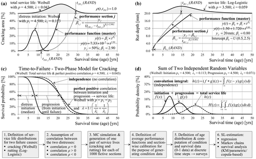
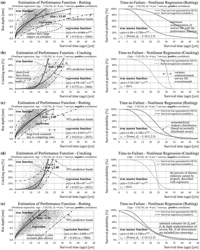
Furthermore, the distress progression and the intermediate conditions until failure can be described with a power function – an approach based on the Hoffmann-process (Hoffmann and Donev 2015, Hoffmann and Donev 2016). The power parameter β ₂ is assumed to be characteristic for each distress type and constant for all sections. In contrast, the scale parameter β ₁ represents the different rate of distress progression among different sections. The parameter β ₁ is estimated using β ₂ (2.90), the condition threshold y _f (50%) and the generated section-specific total service life t _CR,j together with initiation time t _INI,j (Figure 4(a)). Thus, the extent of cracking can be computed for each section at any time. The same procedure is applied for the distress type rutting but without initiation process (Figure 4(b)). The service life is based on a log-logistic distribution (arbitrary) with the corresponding assumptions for β ₂ (0.80) and y _f (20 mm). However, a different set of random numbers was used this time. One difference is that the power function for rutting also includes an intercept term (β ₀), which is assumed to be uniformly distributed among sections. The assumed parameters of the service-life distributions and performance functions are selected to be in accordance with the existing literature. However, it is important to point out that the aim here is to generate data as a basis for a thorough comparison of methods and analysis of resulting bias. Thus, the paper provides readers with the knowledge and means to obtain less biased results from their real world data but draws no conclusions on actual service lives of random pavement data as (out of scope). As a next step, age (i.e. the explanatory variable in the performance function) is generated for each section using a uniform distribution (Figure 5). Consequently cracking area and rut depth are calculated for (seven) different discrete moments in time starting from t ₀ representing consecutive condition surveys. The computations are carried out for three different survey intervals and three different age distributions. The age distribution with a negative minimum value represents an unbalanced panel, since each section is observed for a different number of times and only half of the sections are constructed at time t ₀. However, the analysis is further conducted using age as the time scale, even though sections reach the same age at different calendar times.

Figure 5. Generation of different age distributions (uniform). Definition of survival time as time from construction until failure with the corresponding transformation to age as the time scale.

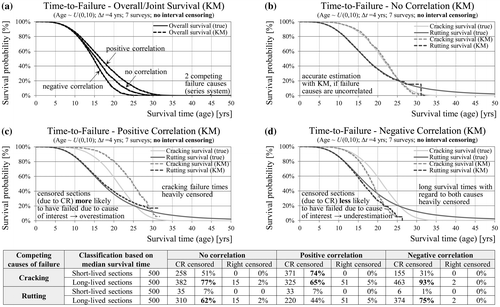
Until now the question about the relationship between cracking and rutting failure times at section level has been neglected here. This study considers three different cases of dependence between the two types of distress illustrated by the scatter plots in Figure 6. The first case assumes independence between service life with regard to rutting and cracking (Figure 6(a)). It must be noted that independence implies zero correlation, but the converse does not necessarily hold true. The second case, as shown in Figure 6(b), is based on mechanistic principles suggesting negative dependence (Smith et al. 2007, Ozer et al. 2016). In practice stiffer asphalt binders are associated with higher cracking potential but better resistance to rutting. Less stiff asphalt binders are more prone to rutting but less susceptible to cracking. The dynamic shear rheometer is used for testing the cracking and rutting potential of asphalt binder under laboratory conditions (Mallick and El-Korchi 2013). The third case of positive dependence has no meaning for these failure types from a mechanistic point of view, but it is considered for reasons of comparison (Figure 6(c)). However, most distresses are expected to be positively correlated, because they share common influencing factors. It is important to point out that the used marginal lifetime distributions for the distress types cracking (Weibull) and rutting (log-logistic) are the same in all three cases. The main difference relates to the ordering of the failure times for individual sections. Thus, in the case of negative correlation, long-lived sections in regard to cracking are more likely to be short-lived in regard to rutting and vice versa.

Figure 6. Scatter-plot of the generated rutting vs. cracking survival times given the same marginal (distress-specific) distributions, but different correlation. Modelling the overall (system) pavement survival as a series system or as a composite index aggregating single distresses (standard approach).

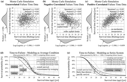
In a situation with competing failure causes the time until a first failure (i.e. the overall survival) might be of interest. Common PMSs use rating and aggregation procedures of subjective nature in order to obtain one total condition for the road section as a basis for the optimisation of treatments. In these systems, as a first step, distress extent or severity are converted into a dimensionless index (school grade) using distress-specific rating scales. In a second step these ratings for different distresses are weighted and combined into one single overall condition index (Hoffmann and Donev 2016). In this example the indices for cracking and rutting are combined by taking the arithmetic average. Alternatively, the pavement as a whole might be modelled with the joint survival function, or what is known as a series system in reliability theory (Figure 6(e)). In that case the joint (system/overall) survival depends on the correlation between the two distresses and falls below the marginal survival probabilities in all three cases with negative correlation leading to the most unfavourable outcomes. As shown in Figure 6(d), the overall survival based on the arithmetic average leads to an overestimation of service life in comparison to the true series-system survival. This holds true even for a different combination of distress weights and marginal distributions. Thus, a systematic overestimation of service life and underestimation of M&R costs is to be expected in any PMS using such overall condition index in the objective function for optimisation (Donev and Hoffmann, 2016).

2.2. Non-linear regression and performance prediction

Observations in the generated data-sets are already left- and right-censored depending on the age distribution. All failed sections are interval-censored because of the survey intervals. The next step is to artificially censor sections due to competing risks. With competing risks only the earliest (first) failure can be observed and failures due to other causes are treated as censored. This holds true if reaching a defined failure threshold for cracking or rutting triggers an immediate application of a treatment restoring or improving the condition. In reality, treatments may be applied only after actually observing the failure (i.e. after periodic surveys) or based on an accurate prediction model at the section level. Furthermore, the pavement may fail due to two causes occurring simultaneously or one after the other (especially in the case of positive correlation). In this paper it is assumed that failures can occur due to only one cause at a time and section, but the problem is quite complex even with this minor simplification.

A standard approach in PMS consists of fitting a regression function to observed continuous data (Figure 7) using the ordinary least squares (OLS) method (Wooldridge 2013). In a regression model the dependent variable is not service life but condition y(t) with censoring affecting the condition distribution. For example, in the case of rutting all observations ≥ 20 mm (failure threshold) are censored. In addition, on sections where cracking failure precedes rutting failure, all rutting observations after the cracking failure are censored (competing event). In the case of positive correlation (Figure 7(a) and (b)) short-lived sections have in average fewer uncensored observations until failure, resulting in enormous overestimation of the service life for rutting and cracking (+15 and +10 years, respectively). In the case of negative correlation (Figure 7(c) and (d)) long-lived sections with respect to rutting and cracking are censored as well reducing the overall bias. Figure 7(e) shows that using all observations beyond the failure threshold (no censoring) in regression analysis leads to less biased results (unbiased intercept and power parameter). Furthermore, prediction intervals, condition distribution and survival function can be estimated under the assumption of normally distributed error terms allowing for a comparison with the true survival function. In summary, standard regression analysis (OLS) does not account for data censoring resulting in biased performance functions and service-life estimates. Moreover, the process of crack initiation cannot be properly modelled with regression analysis leading to additional bias.

Figure 7. Estimation of performance and survival functions with non-linear regression using the generated (censored) condition data and resulting bias with respect to true marginal distributions, mean lifetimes and performance functions.

2.3. Homogeneous Markov chains

Markov chains are a class of stochastic processes describing the transitions of a system between a finite number of states, where the future evolution of the process depends only on the current state and not on the past history (memoryless property). The transition probabilities may be assumed constant (homogeneous) or changing over time (non-homogeneous). Transitions may occur at any time (time continuous) or only at specified time steps (time discrete). The survival time (service life) is defined as the time spent in all states prior to entering the absorbing state. An absorbing state is the failure state (≥ y _f ), from which no further transitions to other states are possible (no treatments). Computational details for Markov chains can be found in the literature and are not provided here (e.g. Crowder 2012, Ross 2014). Figure 8 illustrates a relationship between Markov chains and survival analysis based on a simple two-state (failure/non-failure) inhomogeneous Markov chain (Aalen et al. 2008). The survival probability is equal to the transition probability of remaining in a non-failure state p ₀₀(t). The transition probability for the complementary failure event is the cumulative distribution function F(t). The transition intensity (i.e. the rate at which transitions occur) of changing state q ₀₁(t) correspond to the hazard function h(t). Moreover, in the case of constant transition probabilities and continuous time, the time spent in a non-failure state (i.e. sojourn time) is exponentially distributed with parameter ‒q ₀₀. Thus, the survival time in the two-state homogeneous Markov chain follows an exponential distribution with constant hazard function over time.

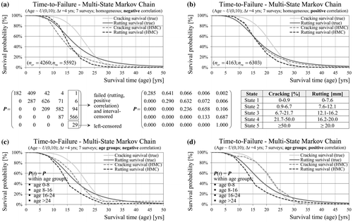
Figure 8. Relationship between survival analysis and Markov chains based on the example of a two-state (a, b) and a competing-risks (c, d) Markov chain.

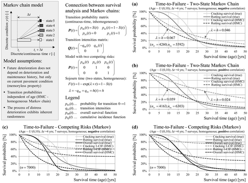
Figure 8(a) and (b) provide an application of such a two-state homogeneous Markov chain model to the generated distress data with resulting survival functions. The computation is based on the full set of 7 surveys (continuous condition) and 4 years inspection interval (transition step). For a section where failure has occurred due to one cause, further observations of all other distress types are censored (competing risk censoring). The transition probabilities are estimated by counting of sections. In the case of negative and positive correlation the deviations from the true model are enormous due to the inflexibility of the exponential distribution. In the case of negative correlation the estimated hazards are higher.

The Markov chain model can be formulated as a competing-risks model with more than one absorbing state (Figure 8(c) and (d)). The probability of remaining in a non-failure state is defined as overall survival function. The transition probability of reaching one failure type is defined as cumulative incidence function (CIF) for this type but has limited practical value (see Section 3.3). An improvement of the resulting estimates of service life may be achieved by using information about the condition states prior to failure. Figure 9(a) and (b) shows a multi-state model with five condition states based on a rating scale. At this point it has to be noted that Markov chain models do not account for interval censoring and dependencies between competing failure causes. Left-censored observations are included in the absorbing state, which therefore plays no role in the computation. Observations of right-censored sections are included in the estimation of the transition probabilities but the model does not explicitly account for right-censoring either. The example also shows that the number of states has a significant impact on the predicted service life. However, any approach for state classification based on rating scale or else is more or less arbitrary. Despite these shortcomings further slight improvements of model accuracy can be achieved by calculation of separate transition matrices for different age groups quite similar to cohort models (Figure 9(c) and (d)).

Figure 9. Survival probabilities based on a five-state Markov chain with transition probabilities being constant for the full analysis period (a, b) or within age groups (c, d).

The Markov chain approach is popular because it allows for modelling of M&R treatments and the use of standard optimisation techniques (dynamic programming). An often made assumption is that within one transition the condition will remain in the current state or will change to next worse state (Butt et al. 1987, Abaza 2017). Although this assumption seems plausible, it is often made without justification in order to reduce the number of unknown probabilities and to simplify the computations. In general, limitations of Markov models include cumbersome estimation of transition probability matrices, small number of observed transitions to states with poorer condition and no section-specific prediction. Explanatory variables may be considered only by further segmentation of the observations in homogeneous groups at the cost of reducing the sample size (Madanat et al. 1995). Furthermore, the assumption of constant transition probabilities in the homogeneous case does not hold true for pavement deterioration due to cumulative traffic and ageing (Li et al. 1996, Abaza 2017, Hoffmann and Donev 2016).

3. Survival analysis for estimation of service life

3.1. Survival analysis in the absence of competing risks

In this section mathematical models accounting for censoring are applied to the generated data. At first it is assumed that failure may occur only due to cracking (i.e. no competing risks). The aim is to investigate the influence of survey interval, number of surveys, age distribution and censoring pattern on the estimation accuracy under ceteris paribus conditions with the non-parametric Kaplan–Meier method. Figure 10(a) and (b) show that wider survey intervals and a higher number of surveys are desirable to obtain a complete estimate of the survival function, but also increase the share of interval-censored sections. Furthermore, Figure 10(c) shows that fitting a parametric Weibull model accounting for interval censoring results in unbiased estimate of the survival function. However, incorrect assumption regarding the distribution (e.g. log-logistic) for cracking lifetime leads to bias (in the lower tail) of the survival function. Using only failed sections and ignoring interval censoring as well results in an underestimation of service life. Figure 10(d) shows that different age distributions are associated with different amount of sections being left-, interval- and right-censored. The age distribution U(030) generates a considerable amount of already failed sections (33%) leading to overestimation, since KM cannot accommodate left-censoring.

Figure 10. KM estimates of cracking survival time in the absence of competing risks - influence of survey interval length (a), number of consecutive surveys (b), assumed lifetime distribution (c), age distribution (d) and (in)dependence of the censoring mechanism (e, f).

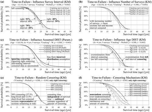
The censoring process may be modelled by two random variables T and C representing the distribution of the failure times and the censoring times, respectively. Thus, for each section only the minimum of the two variables can be observed. In this case the data will only consist of uncensored and right-censored observations making KM an appropriate estimation method. Figure 10(e) shows the special case where the two random variables are statistically independent. Depending on parameters of both distributions, different shares of sections will be censored. However, this does not affect the survival function estimate, which is unbiased even with 80% of the sections being censored. In contrast, if the censoring and failure mechanisms are correlated, the KM estimates will be biased, with direction and size of the bias depending on the sign of the correlation and amount of censoring (Figure 10(f)). This censoring scheme resembles censoring due to dependent competing risks and will be discussed in detail in the next section.

3.2. (Non-)parametric survival analysis in the presence of competing risks

In the next step the two failure types (cracking and rutting) are simultaneously analysed in the cases of independence and positive as well as negative dependence (Figure 11). For the purpose of having only censoring due to competing risks, the generated data is manipulated one more time by replacing all interval-censored observations with the true uncensored lifetimes. Furthermore, with the use of a non-parametric approach any bias due to distribution assumptions will be excluded too. Thus, the overall survival function (failure from any cause) is estimated accurately in all three cases of dependence (Figure 11(a)). Figure 11(b) shows that the KM estimates of the marginal distributions for cracking and rutting are also unbiased, if the assumption of independent competing risks is met (Kleinbaum and Klein 2012). Independence means that sections censored due to the competing event are no more or less likely to fail due to the investigated cause of interest. In the case of positive correlation censored sections are more likely to have failed than those not censored leading to an overestimation of the survival probabilities (Figure 11(c)). In the case of negative correlation short-lived sections with regard to cracking are also long-lived with regard to rutting, and vice versa. Thus, censored sections are less likely to have failed due to the cause of interest resulting in an underestimation of survival probabilities (Figure 11(d)). The size of the under-/overestimation in each case depends on the amount of censored sections and the leading cause of failure.

Figure 11. Unbiased KM estimates (no interval censoring) of joint and marginal (no correlation) survival probabilities (a, b) in contrast to service life over/underestimation in the case of positive/negative correlated competing risks (c, d).

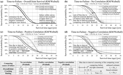
Next, the computations are repeated with the interval-censored data using parametric models. With KM the overall survival function is overestimated in average by 2 years or half of the inspection interval, since the failures are recorded at the upper limit of the interval (Figure 12(a)). The same overestimation is observed for marginal distributions in the case of no correlation (Figure 12(b)). Surprisingly, the estimates with a parametric model are not identical to the true marginal survival functions. The reason for the remaining bias is interval censoring of the competing event. Censored sections due to competing risks are treated as right-censored with the integral of the survival function as contribution to the likelihood. The lower limit of this integral is assumed to be the time of the last inspection, but it should be prior to the inspection, because the competing (censoring) event has happened within the inspection interval. The size of this bias is less significant than the bias due to interval censoring of the event of interest because right-censored observations have a smaller contribution to the total likelihood as compared to interval censoring. In the case of rutting additional bias may be present due to the incorrect assumption of a Weibull distribution. In the case of positive correlation (Figure 12(c)) the bias due to interval censoring and bias due to dependent competing risks are in the same direction leading to increased total bias (summation). In contrast, in the case of negative correlation (Figure 12(d)) the bias due to interval censoring is in the opposite direction of the bias due to competing risks leading to a reduction of the total bias (cancellation).

Figure 12. KM/Weibull estimates of the overall (a) and marginal survival probabilities in the case of uncorrelated (b), positive (c) and negative (d) correlated cracking and rutting.

3.3. Cumulative incidence and conditional probability

Estimation of CIFs and conditional probability curves (CPC) is a common approach for competing risk data that does not rely on the independence assumption. For discussion and details see, for example, Pintilie (2006) or Kleinbaum and Klein (2012). The difference between KM and CIF is that CIF considers competing risk events as failures and not as censored observations as in the case of KM. Figure 13(a) shows the calculation of CIF in the case of negative correlated cracking and rutting failures. CIF provide information about the dominant failure cause, but they cannot be interpreted as survival probabilities. CIF are not equivalent to the marginal distributions and cannot be utilised in prediction models and the subsequent optimisation of treatments.

Figure 13. Overview and estimation of cumulative incidence (a) and cumulative probability curves (b, c) based on competing risk data.

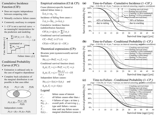
Another concept in SA is the conditional survival defining the probability that a section survives the event of interest given that no competing failure has been experienced. CPC may be estimated based on the CIF estimates. In the case of independent failure causes the marginal and the conditional distributions are identical. In the case of negative correlation (Figure 13(b)) the conditional survival probabilities fall below the marginal survival probabilities, because surviving the competing event makes survival less likely. The opposite relationship can be observed in the case of positive correlation (Figure 13(c)). Even if CPC are estimated without bias, it is not possible to estimate the marginal distribution after the point where the overall survival falls down to 0%.

Yang and Kim (2015) provide the only study known to the authors in pavement management that considers different pavement distress types as competing risks. Unfortunately, the analysis was limited to an estimation of CIF and CPC without acknowledging the limitations of these approaches. Moreover, the nature of possible correlation between the three analysed distresses was not investigated.

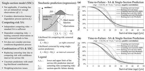
3.4. Performance history-based approach

In summary, traditional survival analysis methods lead to bias in the presence of dependent competing risks. Using information about previous conditions as well as distress progression characteristics has the potential to reduce this bias. A regression function with constant distress progression factor (power factor β ₂) can be fitted at the section level by estimating the scale parameter β ₁ provided that at least three condition observations are available. Since this is the exact same algorithm used for data generation, the performance function will fit perfectly with no deviations (residues). Therefore, a random measurement error is added (subtracted) to (from) each of the observations. Furthermore, condition probability distribution, confidence intervals and failure distribution can be estimated assuming a distribution (e.g. normal) for the error terms (Hoffmann and Donev 2016). The idea is to replace the censoring time for competing-risk censored observations (considered as right-censored) with unbiased upper and lower limits of the confidence interval for the service life derived with regression. Likelihood contributions for failure (censoring) times for the event of interest can be computed as usual without fitting of a regression function. The question how to choose the confidence level for the prediction interval has no correct answer in a mathematical sense. However, confidence levels producing average confidence intervals similar to the inspection interval will ensure that the competing-risk censored sections have no more or less weight in the likelihood than other sections. On the other hand, sections with an unreliable prediction and a wider prediction interval will exhibit a smaller log-likelihood contribution, which is a desirable property.

Figure 14(a) and (b) illustrate the application of this approach to the generated data using single-section regression with a confidence level of 68.2% (one standard deviation of the mean service life). In the case of rutting and cracking (positive correlation) the bias was substantially reduced in comparison to the parametric estimate from Figure 12. The residual bias for rutting is caused by the incorrect distribution assumption (Weibull instead of log-logistic). Nevertheless, in one of the four cases (cracking, negative correlation) the approach was not able to improve the estimates (Figure 14(a)). The reason for this is that the single-section prediction model could not be applied for roughly 1/3 of the competing-risk censored sections because they had less than three observations. Since this group is not random and not representative, the bias was even increased in the lower tail of the survival function in this case. In summary, using a regression prediction model at the section level in addition to survival analysis has the potential to eliminate or reduce bias due to dependent competing risks, if the model can be applied for the majority of the sections and the assumptions of the single-section prediction model are met.

Figure 14. Improvement of survival estimates for dependent competing risks by using previous conditions and distress progression models at section level in combination with survival analysis in the case of negative (a) and positive (b) correlated distresses.

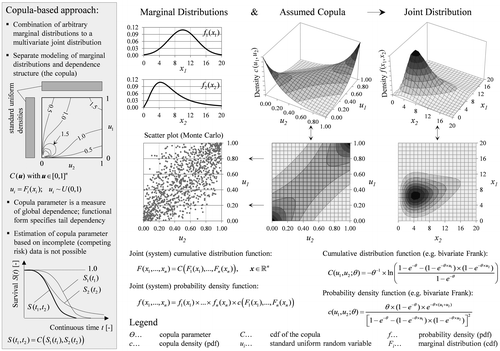
3.5. Copula-based approach

As already shown, if competing risks are independent, the Kaplan–Meier method produces unbiased estimates, but the independence assumption is neither verifiable nor realistic for pavement distress types. Thus, in the presence of dependent competing risks the marginal (latent) lifetime distributions are not identifiable and cannot be estimated without bias with common survival analysis models (Crowder 2012). Moreover, there exists a model with independent competing risks and one or many models with dependent different marginal distributions that produce the same joint (overall) survival function. However, if the dependence structure is known a priori, this identifiability issue can be resolved mathematically. One possibility for a characterisation of dependencies are copula functions providing a way to simultaneously model marginal and joint distributions of random variables. A copula is defined as the multivariate (joint) distribution of standard uniform random variables. Thus, any arbitrary continuous marginal distribution can be uniquely linked to a specific joint distribution using probability integral transformation, if the functional form and parameters of the copula are specified (Figure 15). A description of the mathematical foundations and properties of copulas is beyond the scope of this paper and can be found in the literature (Kurowicka and Cooke 2006, Joe 2015).

Figure 15. Combination of arbitrary marginal distributions to a multivariate joint distribution using copula (dependence) function.

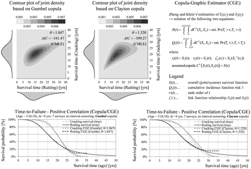
The overall survival function and the CIFs can be estimated from the observed competing risk data. Given these functions and an assumed copula the marginal distributions can be identified with the copula-graphic estimator (CGE) of Zheng and Klein (1995). Figure 16(a) shows the structure of the generated multivariate data in a 3D histogram which can be used for the selection of an appropriate copula form. Furthermore, three different Archimedean copulas are fitted to the uncensored generated data using canonical maximum likelihood (Figure 16(b) and (c)). Finally, the marginal distributions are estimated non-parametrically based on a Frank copula using CGE. The estimates are largely identical to the true survival distributions in both cases of negative and positive dependence (Figure 16 (d)). Figure 17 shows that marginal survival estimates with the flexible Frank copula exhibit almost no bias compared to other forms (Gumbel, Clayton). A critical factor for estimation accuracy is the copula parameter provided that a flexible functional form is selected. This approach may also be generalised to more than two competing risks and extended to a regression model with covariates (Lo 2015). However, in contrast to the performance history-based approach (Section 3.4), the complexity increases substantially when considering more than two failure types.

Figure 16. Histrogram of the generated service life data (a), perspective (b) and contour plots (c) of the joint survival density based on a fitted Frank copula to the true data. Estimation of the marginal survival functions with the competing risk data and an assumed (fitted) copula using copula-graphic estimator (d).

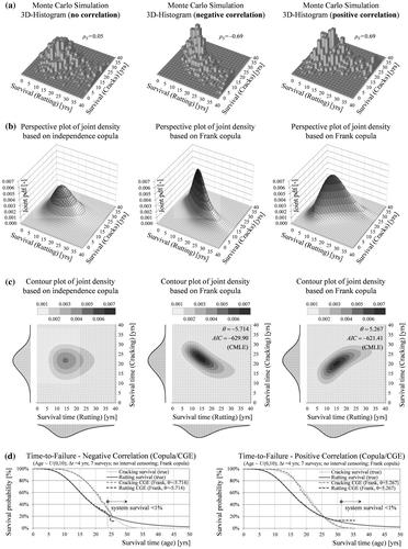
Figure 17. Definition of the copula-graphic estimator and sensitivity of the survival estimates to the functional form of the copula.

Another limitation of the copula-based competing risk approach is that the copula cannot be estimated from the censored data and must be assumed. Laboratory tests and accelerated pavement testing may provide insights about the sign and degree of correlation between different asphalt failure mechanisms. Another approach would be to estimate the survival times until lower condition thresholds (i.e. closer to the initial state) guaranteeing less censored observations. The distress correlation is invariant to this scaling of the survival distribution allowing for the copula to be fitted. In any case further research should be aimed at investigating the dependencies between dominant failure causes from real-world survey data.

4. Conclusions

Reliable pavement performance models are crucial for the planning of maintenance and rehabilitation activities and an efficient use of public funds. For a specific selection and optimisation of treatments performance prediction models and service life estimates for each distress type are needed. The parameters of these models should be estimated with empirical data from periodic condition surveys. Due to the nature of pavement deterioration processes and practical limits of the inspection process, censoring of the data is unavoidable. There are different types of censoring, each showing a different impact on the estimation and a different frequency of occurrence. Approaches like regression analysis (OLS) or Markov chains do not account for censoring. Using them to develop distress progression models may result in substantial bias and more or less arbitrary estimates. Some researchers have used standard non-, semi- and full parametric survival analyses accounting for censoring, but their analyses was limited to the univariate case of only one possible failure type neglecting competing risk and correlation between failure causes. This study covers common cases for pavements exhibiting more than one distress type. Despite the fact that the presented models are in principle capable of accounting for covariates, the related aspects are not included in the paper. Using multiple explanatory variables leads to many issues (e.g. endogeneity bias, multicollinearity, ex-ante prediction, specification errors, etc.) that will be covered in another paper.

Distress modelling in the presence of dependent competing risks poses a challenge, but the reality of more than two and not necessarily mutually exclusive failure causes is even more complex. This paper provides evidence that models with better fit to real-world survey data (e.g. regression) are not necessarily models describing the underlying (unobserved) degradation process and service life accurately. As the ‘true’ degradation process on the network level cannot be observed it is not possible to determine directly which method or model will perform better than others. Therefore, the analysis and conclusions in this paper are based on simulated data allowing a comprehensive and objective comparison of different models to the a priori specified true processes. Based on the results it can be shown that common survival analysis models show substantial bias in the simple case of two positive or negative dependent competing risks. Depending on the present types of censoring and violated assumptions related deviations may partly cancel each other out or add up. Moreover, competing risk approaches based on cumulative incidence reflect the observed data but not the underlying process (marginal distribution). It can be shown that further improvements and bias corrections are achieved by using prior conditions and degradation history at the section level. Another finding is that copulas are a promising alternative for multivariate simultaneous modelling of distress types allowing for an accurate estimation of marginal lifetime distributions with censored data and assumed (estimated) copula parameter. Future research will be concentrated on the comparative application of the presented models and methods to real-world data and the impact of dependence structures between failure causes on estimation accuracy.

Disclosure statement

No potential conflict of interest was reported by the authors.

References

- Aalen, O.O. , Borgan, Ø. and Gjessing, H.K , 2008. Survival and event history analysis. A process point of view . New York, NY: Springer.
- Abaza, K.A. , 2017. Empirical approach for estimating the pavement transition probabilities used in non-homogenous Markov chains. International Journal of Pavement Engineering , 18 (2), 128–137.
- Butt, A.A. , et al. , 1987. Pavement performance prediction model using the Markov process. Transportation Research Record: Journal of the Transportation Research Board , 1123, 12–19.
- Christofa, E.M. and Madanat, S.M. , 2010. Development of pavement cracking initiation models by combining experimental and field data. 89th annual meeting of the transportation research board , 10–14 January, Washington, DC.
- Crowder, M.J. , 2012. Multivariate survival analysis and competing risks . Boca Raton, FL: Chapman & Hall/CRC Press.10.1201/CHTEXSTASCI
- Donev, V. and Hoffmann, M. , 2016. Pavement performance prediction and estimation of service life in the presence of censored condition data. In: Proceedings of the eight international conference on maintenance and rehabilitation of pavements , 27–29 July 2016 Singapore. Singapore: Research Publishing, 680–689.
- Dong, Q. and Huang, B. , 2015. Failure probability of resurfaced preventive maintenance treatments: investigation into long-term pavement performance program. Transportation Research Record: Journal of the Transportation Research Board , 2481, 65–74.10.3141/2481-09
- Hoffmann, M. and Donev, V. , 2015. Probabilistic modeling of flexible pavement performance and LCC – based service lives with failure distributions. In: H. Furuta , D.M. Frangopol and M. Akiyama , eds. Life-cycle of structural systems: design, assessment, maintenance and management , 16–19 November 2014 Tokio. London: Taylor & Francis, 1981–1988.
- Hoffmann, M. and Donev, V. , 2016. Introduction of a new continuous time and state space stochastic process in condition prediction. International Journal of Pavement Engineering . https://doi.org/10.1080/10298436.2016.1162304.
- Joe, H. , 2015. Dependence modeling with copulas . Boca Raton, FL: Chapman & Hall/CRC Press.
- Kalbfleisch, J.D. and Prentice, R.L. , 2002. The statistical analysis of failure time data . 2nd ed. Hoboken, NJ: Wiley.10.1002/9781118032985
- Kargah-Ostadi, N. and Stoffels, S.M. , 2015. Framework for development and comprehensive comparison of empirical pavement performance models. Journal of Transportation Engineering , 141 (8), 04015012.10.1061/(ASCE)TE.1943-5436.0000779
- Kleinbaum, D.G. and Klein, M. , 2012. Survival analysis: a self-learning text . 3rd ed. New York, NY : Springer.10.1007/978-1-4419-6646-9
- Kurowicka, D. and Cooke, R. , 2006. Uncertainty analysis with high dimensional dependence modelling . Chichester: Wiley.10.1002/0470863072
- Li, N. , Xie, W. and Haas, R. , 1996. Reliability-based processing of Markov chains for modeling pavement network deterioration. Transportation Research Record: Journal of the Transportation Research Board , 1524, 203–213.10.3141/1524-24
- Lo, S.M.S. , 2015. Competing risks model and copula . Dissertation (PhD). University of Freiburg.
- Loizos, A. and Karlaftis, M. , 2005. Pavement crack initiation prediction from in-service pavements: a duration model approach. Transportation Research Record: Journal of the Transportation Research Board , 1940, 38–42.10.3141/1940-05
- Madanat, S. , Mishalani, R. and Ibrahim, W.H.W. , 1995. Estimation of infrastructure transition probabilities from condition rating data. Journal of Infrastructure Systems , 1 (2), 120–125.10.1061/(ASCE)1076-0342(1995)1:2(120)
- Mallick, R. and El-Korchi, T. , 2013. Pavement engineering: principles and practice . 2nd ed. Boca Ranton, FL: CRC Press.
- Molzer, C. , et al. , 2000. Statistische Methoden zur Auswertung von Straßenzustandsdaten [Statistics for pavement performance modeling]. Wien: BMVIT, Straßenforschung Heft 499 (in German).
- Nakat, Z.S. and Madanat, S.M. , 2008. Stochastic duration modeling of pavement overlay crack initiation. Journal of Infrastructure Systems , 14 (3), 185–192.10.1061/(ASCE)1076-0342(2008)14:3(185)
- Norouzi, A. , Kim, D. and Kim, Y.R. , 2016. Numerical evaluation of pavement design parameters for the fatigue cracking and rutting performance of asphalt pavements. Materials and Structures , 49 (9), 3619–3634.10.1617/s11527-015-0744-x
- Ozer, H. , et al. , 2016. Fracture characterization of asphalt mixtures with high recycled content using Illinois semicircular bending test method and flexibility index. Transportation Research Record: Journal of the Transportation Research Board , 2575, 130–137.10.3141/2575-14
- Paterson, W.D.O. , 1987. Road deterioration and maintenance effects: models for planning and management . Baltimore, MD : The Johns Hopkins University Press.
- Pintilie, M. , 2006. Competing risks: a practical perspective . 1st ed. Chichester: Wiley.10.1002/9780470870709
- Prozzi, J.A. and Madanat, S.M. , 2000. Using duration models to analyze experimental pavement failure data. Transportation Research Record: Journal of the Transportation Research Board , 1699, 87–94.10.3141/1699-12
- Reger, D. , et al. , 2013. Estimation of pavement crack initiation models by combining experimental and field data. Journal of Infrastructure Systems , 19 (4), 434–441.10.1061/(ASCE)IS.1943-555X.0000148
- Ross, S.M. , 2014. Introduction to probability models . 11th ed. Waltham, MA: Academic Press.
- Rübensam, J. , et al. , 2005. Untersuchungen zur Wirtschaftlichkeit und bautechnischen Bewährung von Fahrbahnbefestigungen aus Asphalt und Beton auf bestehenden Bundesautobahnen [Investigations of the profitability and structural dependability of asphalt and concrete carriageway pavement on existent interstate highways]. Bonn: Forschung Straßenbau und Straßenverkehrstechnik, Heft 914 (in German).
- Schram, S. and Abdelrahman, M. , 2009. Mechanistic-empirical modeling in network-level pavement management. Transportation Research Record: Journal of the Transportation Research Board , 2093, 76–83.10.3141/2093-09
- Shin, H.C. and Madanat, S. , 2003. Development of stochastic model of pavement distress initiation. Journal of Infrastructure Planning and Management , 744 (61), 61–67.
- Smith, A.F. , et al. , 2007. TexSys: guide for selecting HMA for Texas flexible pavements . El Paso, TX: Center for Transportation and Infrastructure Systems, University of Texas at El Paso.
- Van Dam, T.J. , Chesher, A.D. and Peshkin, D.G. , 1997. Evaluation of LTTP data using HDM-III probabilistic failure-time models for crack initiation in bituminous pavements. Transportation Research Record: Journal of the Transportation Research Board , 1592, 125–133.10.3141/1592-15
- Wang, Y. , Mahboub, K.C. and Hancher, D.E. , 2005. Survival analysis of fatigue cracking for flexible pavements based on long-term pavement performance data. Journal of Transportation Engineering , 131 (8), 608–616.10.1061/(ASCE)0733-947X(2005)131:8(608)
- Wooldridge, J. , 2013. Introductory econometrics: a modern approach . 5th ed. Mason, OH: South-Western Cengage Learning.
- Yang, J. and Kim, S.H. , 2015. Investigating the performance of as-built and overlaid pavements: a competing risks approach. International Journal of Pavement Engineering , 16 (3), 191–197.10.1080/10298436.2014.937808
- Zheng, M. and Klein, J.P. , 1995. Estimates of marginal survival for dependent competing risks based on an assumed copula. Biometrika , 82 (1), 127–138.10.1093/biomet/82.1.127