Optimisation of pavement maintenance and rehabilitation activities, timing and work zones for short survey sections and multiple distress types

ABSTRACT

Existing pavement management systems (PMSs) aggregate short survey sections into long homogeneous sections (typically 1–5 km), aiming to reduce the amount of data and formulate a tractable optimisation problem. However, assuming that sections in a similar condition will undergo a similar deterioration of this condition is incorrect, resulting in imprecise predictions and violations of thresholds. Thus, any maintenance and rehabilitation (M&R) optimisation approach based on long road sections and a single condition indicator (aggregated or not) cannot provide applicable results at the project level. This paper provides a holistic model framework and consistent methodology for a new PMS, abolishing the need for composite condition indices, data aggregation and homogeneous sections in the M&R optimisation process. The proposed bottom-up optimisation is based on short survey sections (25–50m) and solves for optimal treatment type, timing, work-zone length and layout, minimising agency, road user and environmental life cycle costs. Instead of using just one condition indicator, the method models the effects of each treatment on multiple distress types and their combinations. Moreover, the short survey sections are grouped into larger work zones based on purely economic criteria (i.e. economies-of-scale costs). Treatment cost, temporary traffic control cost, and work-zone user cost models are derived as a function of the project size and calibrated for actual prices in Austria. Genetic algorithms are employed as a part of the solution algorithm, being capable of handling an unlimited number of road sections. Furthermore, the approach can be extended to account for budget restrictions, risk and cross-asset allocation of funds for any aging repairable infrastructure system.

KEYWORDS:

• Pavement management
• bottom-up optimisation
• life-cycle costs
• work-zone length
• M&R strategies
• economies of scale
• genetic algorithms
• freeways

1. Introduction

Pavement management covers the processes of data collection, condition assessment and prediction, planning, optimisation and application of maintenance and rehabilitation (M&R) treatments, as well as budgeting. The objective of M&R optimisation is to maximise performance (e.g. network condition), or to minimise agency and user costs, or to minimise risk/environmental impacts by selecting appropriate treatments (decision variables), subject to constraints (e.g. budget). This problem can be formulated for a single road section (single facility), for a travel route consisting of multiple sections, or for the entire network (system) covering all sections and other road assets.

In the context of aging infrastructure, increasing traffic loads, demanding public expectations and limited budgets, road agencies in developed countries are faced with several requirements. They have to maintain the network condition, allocating their budget according to the needs by balancing trade-offs between agency and user costs in the long term, but also to reduce accidents, emissions and traffic flow interruptions in the short term. An ideal pavement management system (PMS) would therefore address these goals simultaneously, providing optimal budgets at the network level, as well as detailed location-specific treatment recommendations in terms of timing, type, work-zone length and layout that could be accepted by road engineers and applied with limited need for manual adaptation.

Common PMSs aggregate short survey sections to long homogeneous sections based on different algorithms, effectively resulting in an averaging of measured condition data. The purpose of this approach is to reduce the computing effort and the complexity of the optimisation problem. However, there is a growing discrepancy between the on-going development of automated condition survey systems (laser technology), delivering more accurate measurements with higher resolution and collection frequency, sharply contrasting with the limited capabilities of current PMS, using only a fraction of the provided information in prediction and optimisation.

Surprisingly, the validity of the approaches for sectioning and data aggregation is not questioned in the literature and the consequences of their use are not investigated. The assumption that a similar condition (at the time of the survey) implies similar future deterioration is proven wrong by empirical research. Thus, condition predictions based on homogeneous sections cannot be accurate. Moreover, the defined condition thresholds are systematically violated due to averaging effects, and it is not possible to select optimal work zones since the formation of homogeneous sections is conducted prior to prediction and optimisation.

This paper provides a holistic framework and methodology for an end-to-end PMS which does not rely on homogeneous sections and composite condition indices. The foundations for this system are laid by deriving calibrated cost, performance and duration models which are shortly presented in the paper as well. The core, however, is the new optimisation approach which is based on short survey sections (e.g. 50 m), allowing for precise condition predictions and section-specific treatment recommendations. The developed optimisation algorithm groups the short survey sections into longer work zones based on economies-of-scale costs. The application of this new methodology is demonstrated by using a case study of 1000 road sections, realistic condition data, as well as multiple distress types and treatments.

The following section (Section 2) gives an overview of the relevant literature by focusing on the shortcomings of common approaches. Section 3 introduces the case study, the calibration of the input parameters as well as the developed performance and cost models. The methodology of the optimisation approach and the results of its application are presented in Section 4 and Section 5, respectively. The explicit mathematical formulation of the optimisation model and the details of the solution algorithm are briefly explained, while an in-depth description will be the subject of another paper.

2. Literature review

There is extensive literature on the topic of pavement M&R optimisation. However, most authors approach the problem from different perspectives by focusing only on a single section at the project level, budget allocation at the network level or work-zone scheduling. The research on budget allocation is concerned with long-term performance and selection of M&R strategies, using either prioritisation or optimisation algorithms, but usually does not consider the network configuration or the planning of work zones. The literature on work-zone optimisation considers trade-offs between one-time agency and work-zone user costs but does not optimise treatment type and timing within a comprehensive life cycle costing approach.

Typical prioritisation methods, such as the marginal cost-effectiveness (MCE) approach, are widely used, despite the need for composite condition indices and being inferior to optimisation (Haas et al. 1994, AASHTO 2012). The MCE approach, however, suffers from a few additional drawbacks. First, maximising effectiveness as an objective favours reconstruction and heavy rehabilitation (larger area between the curves) and may produce significantly higher agency costs (only included as a constraint). Second, the computation of effectiveness based on an aggregated index is problematic because the results of the optimisation depend on the aggregation rules and weights, and are therefore subjective.

2.1. Budget allocation and optimisation based on life-cycle costs

In contrast to prioritisation, mathematical optimisation allows for an optimal (near-optimal) solution to be found in the case of exact (heuristic) methods. Moreover, multiple constraints (e.g. annual budget, condition, level of service, etc.) can be incorporated in the formulation of the problem. Two basic approaches are discussed in the literature: top-down and bottom-up. Top-down methods analyse road sections in groups (discrete classes) and treat all sections in a group as identical in terms of deterioration (e.g. Kuhn and Madanat 2005). In this way, these methods are independent of the number of road sections and thus very efficient for large-scale networks. The disadvantage is that all sections in a class receive the same treatment and section-specific recommendations cannot be given.

In contrast, bottom-up approaches consider section-specific distress information and deterioration rates. Bottom-up optimisation can be further divided into one-stage and two-stage solution approaches. One-stage bottom-up approaches consider all possible combinations of road sections, M&R treatment types and application years simultaneously. Each combination is represented by a binary decision variable that takes the value ‘1’ if the treatment is selected and ‘0’ otherwise. The goal is to minimise the discounted total life-cycle costs, subject to budget and condition constraints. The problem cannot be solved exactly, even for a very small number of sections, due to the exponential complexity and inevitable nonlinearities in the objective function. Hence, many authors have adopted a heuristic technique (genetic algorithm) in their solution (Fwa et al. 1996, Ferreira et al. 2002, Santos et al. 2017). However, the major drawback of these approaches is that there is no guarantee and no way to know whether the obtained M&R programme is even close to optimal (for large networks).

Two-stage bottom-up approaches consist of selecting a small set of optimal and sub-optimal M&R strategies for each section. Based on this selection, the objective is to find the optimal combination of strategies at the network level, satisfying the budget constraint in each year. Yeo et al. (2013) and Lee and Madanat (2015) formulate the network-level problem as a constrained combinatorial problem, which they solve with evolutionary algorithm or pattern search heuristic. These models represent pavement condition by using only one indicator, namely the pavement serviceability rating or the international roughness index (IRI), respectively. In reality, however, pavements exhibit various types of distress that may require different treatments in each case. One advantage of the two-stage approaches is that the optimal strategy for each section provides the solution at the network level, if the budget constraint is not binding, which could be used as an orientation value for the constrained problem.

2.2. Optimisation of work zones

The literature on work-zone scheduling is mostly concerned with operational decisions for short-term work zones by optimising project length, duration, traffic control and starting time (e.g. Chien and Schonfeld 2001, Jiang and Adeli 2003). The optimisation is based on the trade-off between economies-of-scale agency costs and work-zone impacts in terms of delays and accident costs. These costs only comprise one-time (initial) costs, with life-cycle costs and future treatments being neglected. Moreover, the analysis focuses only on single projects, where treatment type and timing have already been determined.

As a step forward, these models were extended to account for future costs with a very simplified life cycle (Chen and Schonfeld 2007, Yang 2010). The authors investigate trade-offs between longer service life (resurfacing interval) and higher one-time agency and user costs for thicker pavements. Thereby, resurfacing interval is a linear function of the decision variable overlay thickness. Then again, these studies focus only on a single project with no optimisation of treatment timing or type and no true life cycle.

Hajdin and Lindenmann (2007) consider multiple projects based on a graph model of the network. M&R treatments on pavement sections and other road assets (bridges, tunnels) are grouped into larger work zones which minimise long-term costs, subject to budget constraints. The main limitation of this approach is its reliance on static input from external management systems which determine M&R strategies (optimal and alternatives) independently for each individual asset. Subsequently, the proposed network optimisation considers only those treatments which are scheduled within a single budget period. However, a joint optimisation of work-zone length and M&R timing for all assets (and not only for those with treatments in the budget period) over a longer period may lead to quite different results. But then again, this would enormously increase the complexity of the proposed model.

Medury and Madanat (2013) incorporate work-zone effects in a bottom-up network-level approach (budget allocation) by defining a network capacity threshold as a constraint. The applicability is demonstrated on the basis of a small case study of 11 road sections. Their model, however, neither accounts for economies-of-scale costs nor for different traffic demand on individual sections.

In summary, most of the approaches used in the literature are not scalable for large networks due to complexity issues. The models that are scalable, in turn, include too many simplifications to yield detailed applicable results at the project level. Apart from the mentioned limitations, almost all of the studies referred to above are based on road sections with lengths between 1 and 5 km. Automated condition surveys, however, report data for much shorter survey sections (data segments) (e.g. 10 m in California, 50 m in Austria, 100 m in Germany, etc.). These survey sections are aggregated into homogeneous sections (management segments), with measurements being aggregated to condition variables. These long-used approaches were originally motivated by (i) the storage and processing capabilities of computers at the time, (ii) the exponential complexity of the optimisation problem, and (iii) short sections not being suitable for practical application of treatments. However, the use of homogeneous sections leads to imprecise condition prediction, resulting in over- and underestimating service life on short sections. Imprecise predictions, in turn, lead to imprecise treatment recommendations at the section (project) level. Moreover, long homogeneous sections prevent the selection of work zones based on economies-of-scale costs, reducing the flexibility in the optimisation.

Today, powerful database management systems which are capable of efficiently storing, managing and analysing big data are available, so that the first issue (i) no longer applies. This paper contributes to resolving the second and third issue (ii and iii) by making use of short survey sections which will allow road agencies to benefit from high-quality data obtained by automated surveys.

3. Case study, performance and cost models

3.1. Overview of holistic PMS framework

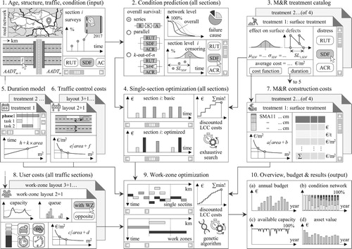
A graphical overview of the new end-to-end PMS incorporating the novel optimisation approach is provided in Figure 1. The figure aims to enhance the understanding of the optimisation framework as a whole, illustrating the flow of information and the different computational steps. Based on a database containing section-specific information (structure, condition, age, traffic, etc.), the first crucial step is predicting the condition for each road section (and each distress type) and deriving a service life/condition distribution at the network level. If condition predictions are biased, the subsequent analysis, treatments and optimisation results will deviate from reality, regardless of the methods applied. Modules 3, 5, 6 and 7 include the developed performance, duration and cost models described in this section. The first stage of optimisation is conducted at the road section level (Section 4.1). The second stage is the optimisation of work zones (Section 4.2), using the results from the first stage as initial values, also considering user costs and traffic control costs. The last stage is the optimisation under budgetary restrictions, leading to less optimal results (as treatments are deferred) and the analysis of obtained results.

Figure 1. Overview of the developed performance, cost, duration and traffic models as modules of a holistic PMS, together with the sequence of computations from input to output.

3.2. Service life with distress and spatial correlation

This section describes the development of the concept and data generation procedure for a case study with a simulated road network replicating real-world data characteristics (Donev and Hoffmann 2017b, Hoffmann and Donev 2017). Simulation studies are used quite often in the research literature on treatment optimisation, especially when demonstrating the applicability of new approaches (e.g. Fwa et al. 1996, Sathaye and Madanat 2012, Yeo et al. 2013). One of the reasons for this is that new approaches have to be tested for a variety of settings, and possible limitations have to be identified prior to any real-world data application. Sensitivity analysis and what-if scenarios help identify key factors, trade-offs and improvement potential of the overall system (e.g. design optimisation, inspection intervals, etc.). Furthermore, a perfect knowledge of service life enables model comparison and objective quantification of the consequences of sectioning and aggregation in terms of threshold violations. This paper offers a general procedure for the simulation of multiple distress types and short survey sections, incorporating spatial correlation based on empirically calibrated input parameters.

The case study is based on 1000 road sections, each with a length of 50 m and located on one of the exterior lanes of a four-lane freeway. All input parameters are calibrated and conceptualised for flexible pavements on freeways in Austria. Other road classes characterised by different design or types of pavements may exhibit different distresses and failure causes. Pavement condition is being modelled by using multiple distress types, with different treatments being possible for different distress combinations. In contrast, many researchers only consider one distress type or aggregate individual distresses into one composite index which is used in the optimisation. Roughness, as measured by the IRI, is perhaps the most common and often the only condition indicator included in optimisation approaches. This is due to the fact that roughness is considered a primary determinant of user costs, and there are many roughness-based performance and user-costs models available in the literature. However, roughness as well as any composite index, is not in itself a failure mechanism but an indicator of several other distress types. Therefore, assigning treatments solely based on composite indices or roughness values fails to address the individual distress types appropriately.

For the purposes of a clear graphical representation of the results, this study considers only three main distress types for asphalt pavements: rutting, surface defects (ravelling, polishing, bleeding, etc.) and alligator (bottom-up fatigue) cracking. However, the complexity of the approach is not affected in any way by the inclusion of more than three distress types, provided that the corresponding condition models are available. Service life with regard to each of these three distress types is assumed to follow its own distribution as shown in Figure 2(a,b). For more flexible modelling, three different distributions are used: the normal, the Weibull and the log-logistic. From a theoretical point of view, the service lives of the three distress types have to be correlated (i.e. correlated random variables). The used correlation coefficients shown in Figure 2(d) are estimated in the course of a preliminary analysis of data based on 1400 km regional roads in Austria (approx. 28,500 road sections). Without any claim to general validity, the assumed matrix is considered a realistic possibility for the purposes of the case study. As expected, the service lives are positively correlated, because most of the distress types share common influencing factors (traffic, climate, etc.). However, the estimated correlation coefficients show that the degree of correlation is not very strong.

Figure 2. Overall service life (a) and dominant failure cause (b) resulting from the distress-specific service life distributions (c) and the correlations between these distributions (d).

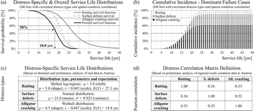
Service life for each distress is defined as the physical time from construction until exceeding a specified condition threshold. The individual distress types are combined in a series system representing the service life of the whole pavement. Thus, on a given section, the individual distresses may be considered as competing risks with the first distress that exceeds its thresholds determining the failure cause and the overall service life. Figure 2(a) shows that the overall service life is on average shorter as the service life of the most critical distress. This follows from the fact that, for a series system, the overall survival probability at any time is the product of the survival probabilities for the individual distress types (in the case of uncorrelated distresses). Details about the estimation of service life with censored data and correlated competing risks can be found in Donev and Hoffmann ( 2017a).

The combination of marginal (distress-specific) distributions and distress-correlation matrix not only defines the overall survival function but also the dominant failure cause given by the cumulative incidence function, as shown on Figure 2(b). In particular, alligator cracking causes 60% of all failures, followed by surface defects with 30% and rutting with 10%. These values are assumed on the basis of the available literature and on the results of network-wide surveys of freeways in Austria (Fromm et al. 2012, unpublished). The parameters of service-life distributions are reverse-engineered based on the assumed failure causes, the estimated distress correlations and a structural life (cracking) of approximately 20 years (FSV, 2016).

So far the spatial arrangement of the road sections has not been taken into account. The assumption of independent condition developments on adjacent sections is unrealistic, as they often exhibit quite similar condition. This study employs a times-series model to account for a positive correlation between adjacent road sections (spatial, serial or autocorrelation). The focus, however, is not on a sequence of observations in time, as it is usual for time series, but on series of ordered measurements at intervals of equal length (survey sections). Thus, a second-order autoregressive process was fitted to real-world data by using conditional maximum likelihood estimation. The basic formulas are shown in Figure 3(d) and for more details on time series, reference to the literature is made (e.g. Hamilton 1994, Montgomery et al. 2015). Condition data of regional roads from two Austrian states was used for this analysis with models being fitted to individual roads. While the mean condition may vary between roads, the estimated autoregressive parameters are relatively consistent with the average values shown in Figure 3(d). The order (i.e. number of lags) of the autoregressive models is determined based on the partial autocorrelogram (Figure 3(c)). For the vast majority of sections, the correlation is significant over a length of one to four sections (50 m length) with two lags being the most common. Furthermore, the results showed that the number of lags and the degree of the correlation depend on the distress type and length of the survey sections (25 m and 50 m were examined). Figure 3(a,b) illustrates the difference between ordered and random sequences of service lives for rutting.

Figure 3. Positive serial correlation (а) vs. no serial correlation (b) of rutting service life for a 3-km road segment with partial autocorrelation function for the two cases (c). Fitting of autoregressive (2) process to real-world data with the estimated autoregressive parameters (d) and graphical representation of the road segment simultaneously exhibiting serial correlation and distress correlation (e).

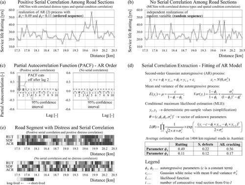
Incorporating spatial correlation will not change the marginal distributions in Figure 2, but will affect the arrangement of the simulated service lives. Generating a data set that simultaneously accounts for distress and spatial correlation, as shown in Figure 3(e), is not straightforward, but a detailed description is beyond the scope of this paper. In short, the procedure consists of the following two steps. First, a set of correlated random numbers is obtained using Cholesky decomposition of the distress correlation matrix (Meissner 2014). In a second step, the spatial correlation is introduced to the same set of correlated random numbers based on the estimated autoregressive parameters. Random variates (service lives) are then obtained by using the inverse-transform method (Rossetti 2016).

The incorporation of spatial correlation is of critical importance as it affects the grouping of adjacent short-survey sections to longer work zones based on economies of scale. The goal here was not to develop a general methodology for modelling of spatial dependence but to generate realistic data set for the case study, also allowing for a ceteris paribus comparison with common approaches. A more accurate and flexible way to account for spatial variability is based on the theory of random fields (Lea and Harvey 2015).

In summary, the simulated road network could be considered as a realistic case study due to the extensive empirical calibration. This not only assigns more weight to the delivered proof of application (see Section 5), but also allows for some practical conclusions to be drawn, which are subject to further investigation.

3.3. M&R treatments: definition and service life

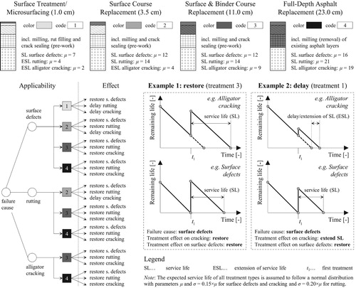
This work assumes a flexible pavement structure which is based on the Austrian design catalogue (FSV 2016) and consists of three asphalt layers (surface, binder and base) as well as two unbound layers (road base and subbase). Accordingly, four M&R treatment types are considered, with each treatment allowing more extensive (deeper) repair of the pavement (Figure 4). Each treatment is represented by a colour code (for visualisation) and an integer code (mathematical model). Since the case study only considers the exterior lane, there is a vertical restriction and the existing pavement height must be maintained. Therefore, all treatments include the removal of the corresponding existing layer(s).

Figure 4. M&R treatment alternatives, characterised by depth of repair, effect (restore/delay) on the different distress types and technical applicability (decision tree).

As will be seen in Section 4.4 of this work, the number of treatment types has a great impact on the complexity of the optimisation problem. Therefore, only a moderate number of M&R alternatives should be considered. Treatments with effect on the same distresses, exhibiting similar service life and costs, can be represented as a group or by the most cost-effective. For example, there are many types of surface treatments: microsurfacing, slurry seal, fog seal, chip seal, ultrathin friction course, and so forth. If the optimisation recommends a surface treatment, then the exact type could be specified at the planning stage based on other factors (e.g. experience, available technology, bidding results). Furthermore, the selection of treatments here represents the most common treatments applied on Austrian freeways. Bearing-capacity problems of the unbound layers, which would require a full-depth pavement replacement, are the exception. Crack sealing and pothole patching are usually considered in the budget for routine (corrective) maintenance and applied on an annual basis or as soon as possible, respectively.

The effect of each treatment on the three modelled distress types is described with a distinct service-life distribution (see Figure 4). Due to the lack of evidence for other functional forms, and for simplicity, it is assumed that the treatment life follows a normal distribution with the mean value based on literature review (e.g. Hall et al. 2001, Cuelho et al. 2006, Anastasopoulos and Mannering 2015, Birbaum 2016, Nobakht et al. 2016). Since the literature rarely distinguishes between effects on different distress types, the values were supplemented using engineering judgment and surveys. The standard deviation is computed as a percentage of the mean value (20% for rutting and 15% otherwise). These values were selected in accordance with the literature and in order to achieve similar distribution of failure causes as compared to the initial service life.

Besides the generated service lives, no continuous distress or improvement model is employed in the current case study. This property ensures a highly robust model which is not dependent on additional assumptions about performance functions. Therefore, service life, defining the latest possible timing of treatment application, is the only information needed. Since all considered treatments apply to the whole area of the lane and no local repairs (patching) are considered, there is no particular benefit in knowing the exact distress extent prior to the threshold. However, if the condition thresholds cannot be satisfied (e.g. due to budgetary restrictions) and the service life is exceeded, a performance model would be necessary to measure the extent of threshold violation. Furthermore, the presented approach can incorporate any mechanistic, empirical or stochastic condition model for the description of intermediate states, with no repercussions as to the complexity of the problem.

In the absence of a performance model, the deterioration is illustrated with the remaining life function, which equals the service life at the time of construction/treatment application and decreases linear to zero at the time of failure (see Figure 4). The model also considers the technical applicability of treatments depending on the failure cause. As illustrated by the decision tree, if the failure cause is alligator cracking, only two treatments can be applied. For the purposes of the case study, it is assumed that rutting is confined within the surface course.

Furthermore, two types of treatment effect are considered: restoration/reset (Example 1) and delay/service life extension (Example 2). The restoration effect is the standard one, and it resets the remaining service life (if any) to the treatment life. For example, if microsurfacing is applied, the service life for surface defects will be reset, but the service lives for rutting and alligator cracking will continue to elapse unaffected. The delay effect, however, assumes that the remaining life for rutting and alligator cracking will be extended by a small amount, shifting the remaining life function horizontally. This assumption is justified by the inclusion of pre-treatment works (crack sealing and rut levelling) in the description of the treatment (microsurfacing).

The treatment life is correlated with the initial service life as well as with the treatment lives on the adjacent road sections. The proposed approach allows for modelling of stochastic treatment lives for the time period after the first treatment when no condition information is yet available. In such cases, deterministic models cannot be calibrated, as customary, using shift or scale factors. Deterministic models will thus predict equal service life, same failure causes and equal treatment intervals for large groups of sections leading to underestimation of M&R needs.

3.4. Agency costs for M&R treatments

The estimation of agency costs for M&R treatments is based on a linear model with fixed and variable cost components. The parameter estimates for the four treatment types are provided in Figure 5 (bottom right) with graphical representation as unit costs and total project costs shown in Figure 5(a,b), respectively. The unit costs decrease with increasing project size due to the spreading of fixed costs over larger work-zone area (economies-of-scale effect). It is not possible to capture these effects with average costs used by many PMSs leading to an over- or underestimation of treatment costs for a given project.

Figure 5. Bottom-up M&R construction cost calculation based on price lists and contractor’s bid prices from Austria. Unit costs (a) and total project costs (b) as a function of the project area for the considered four treatment types.

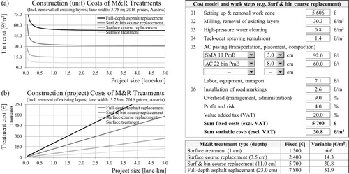
The cost functions are based on detailed bottom-up calculation, a simplified version of which is also shown in Figure 5. The calculation includes the necessary work activities for each treatment, the selection of asphalt mix and thickness, as well as unit prices for each item. The prices for each item are then divided into fixed and variable components and summed up accordingly. The advantage of this bottom-up calculation is its facile adjustment to other regions or countries by using current prices for material, labour, fuel, etc.

The unit cost estimates are based on a comprehensive analysis of contractor’s bid prices for 60 M&R projects in Austria, price lists from asphalt mixing plants, data from road planning offices and available literature (Wießmayer 2006, Lindenmann 2008, Birbaum 2016). All prices were converted to 2016 constant euros using construction price indices for Austria. The costs for setting up and removal of the work zone (often given as a lump sum in bids) cover the following activities: site clearance, office facility setup, power/water supply, material storage, transportation of tools, equipment, machinery, vehicles, scaffolding, and others. The analysis has shown that a large portion of these costs are fixed costs. However, the setup costs not only depend on the treatment type, but on the size and complexity of the project. The cost model accounts for this variable proportion by using empirical relationships, with the project duration as a proxy for size and complexity (Birbaum 2016). If pre-treatment works (crack sealing, rut filling) are considered for a given treatment, their costs are included as well.

3.5. Agency costs for temporary traffic control

Due to extensive work-zone safety measures on freeways with heavy traffic, temporary traffic control costs (TTCCs) represent a large proportion of the total agency costs for M&R projects in Austria and Germany. Naturally, TTCC depend on the work-zone layout and the functional class of the road. Figure 6(a,b) shows two typical configurations for a work zone in the exterior lane of four-lane freeways with the corresponding lane widths, work-zone capacity, speed limit and channelising devices. These layouts are simplified versions of the exemplary traffic management plans for long-term work zones provided in the Austrian standards (FSV 2012). For the estimation of work-zone capacity a base capacity of 2100 veh/h per lane is used, together with capacity reduction factors derived from the literature (Hellmann et al. 2008, Fischer 2009). If the work zone extends over the entire roadway, the construction can be staged with lane closures in sequence shifting traffic from the existing to the newly repaired lane. However, technological and quality considerations may require both lanes to be repaired in a single pass with full-width asphalt paver. In that case, a full roadway closure will be necessary (e.g. layout 3 + 0 or 4 + 0). Each alternative is associated with different agency costs, available roadway capacity and accident risk.

Figure 6. Common exterior-lane work-zone layouts on Austrian freeways (simplified) with corresponding speed limits, channelising devices and roadway capacity values (a,b). TTCCs derived by bottom-up approach as a function of the project length (c,d).

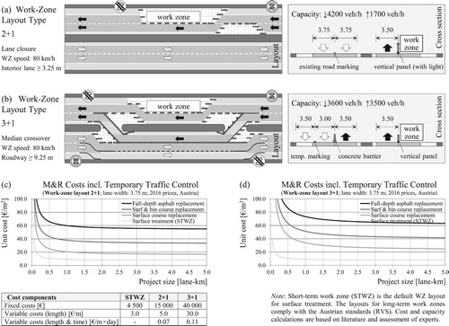
TTCCs are often neglected in the literature on budget allocation (see Section 2.1), as there is no way to attribute these costs without work zones. Moreover, temporary traffic control is sometimes an in-house service, which the agency performs with its own staff. Thus, there is not much literature on the estimation of TTCC, apart from some estimates as a percentage of the project’s total cost. The cost functions for layout 2 + 1 and 3 + 1 given in Figure 6(c,d) are based on data provided in the German literature (Fischer 2009, Birbaum 2016), with adjustment for Austria. The cost functions are based on a more detailed bottom-up cost calculation with unit prices for the different items and services. The fixed component consists of costs for the setup of the work zone approach and transition area, asphalt works for unpaved median strips (where relevant) and installation of lighting devices in crossover areas. Length-dependent variable costs include the delivery/setup of vertical panels separating the worksite from vehicular traffic as well as the installation of temporary markings and traffic signs. Time-dependent costs comprise running costs (e.g. electricity), rental costs (for traffic control devices), surveillance, daily inspections, maintenance, and cleaning. Microsurfacing is applied by a specialised truck- or trailer-mounted mixing and paving machine in a continuous way, which requires a mobile short-term work zone with significantly lower TTCC. In summary, TTCCs are an important component in the agency budget with a high proportion of fixed costs, which is essential for the grouping of work zones.

3.6. Work-zone duration model

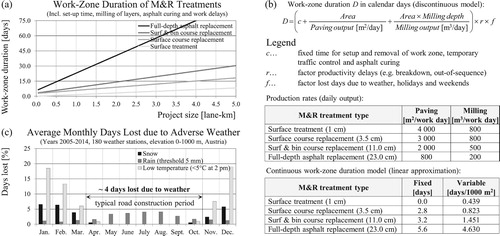
To account for the impact of construction activities on road users as well as time-dependent traffic control costs a treatment duration model is needed. The simplified treatment duration model shown in Figure 7(b) is based on paving and milling production rates and accounts for setup time, delays and adverse weather days. Production rates for an eight-hour workday are selected using literature (Lindenmann 2008, Brozek et al. 2009) and data from manufacturers’ specifications (e.g. Wirtgen 2013). A fixed time for work-zone setup and removal (factor c) is included for each treatment type. Especially for new construction, the setup time will also depend on the size and complexity of the project. The productivity delay factor r is assumed to be equal to 1.2 for M&R works (i.e. 20% increase of project duration), accounting for material- and equipment-related idle times, design changes or errors, poor management, and so forth (Anastasopoulos et al. 2012). Factor f considers days lost due to adverse weather conditions which have an influence on asphalt paving activities (snow, rainfall, low or high temperatures). In order to determine this factor, observations from 180 weather stations in Austria for nine consecutive years were analysed, with the average results shown in Figure 7(c). Region- and month-specific factors could be used in a more detailed model, although the individual analysis of each of the nine Austrian states for two elevation groups (0–500 m and 500–1000 m) showed differences primary in the winter period, when no M&R activities take place. The thresholds defining lost days are based on the Austrian specifications for asphalt paving and suggestions in the literature (Williams et al. 2009). The resulting work-zone duration as a function of the project size for each treatment is graphically represented in Figure 7(a). The linear models represent a very close approximation to the formula, which exhibits discontinuities for a duration of less than five days.

Figure 7. Derivation of the work-zone duration model (a,b) using production rates from the literature and accounting for days lost due to adverse weather conditions based on an extensive analysis of 180 weather stations over nine years in Austria (c).

3.7. Work-zone user and environmental costs

User costs include traffic delay costs (TDC), vehicle operating costs (VOC), emissions costs (EC), and crash costs (CC) according to EU regulations (Eurovignette Directive). In general, a distinction can be made between condition-related and work-zone related user costs. Condition-related user costs are a function of the road condition, with the majority of models linking user costs to roughness (IRI). However, measured IRI values are often not directly comparable between agencies due to differences in equipment, methods, and reporting (Ogwang 2016). Thus, the existing IRI-based models are not always applicable and, in addition, not every agency disposes of sufficient resources in order to develop its own user-cost models. Furthermore, a situation where a poor pavement condition (represented by IRI) will lead to speed reductions and ultimately to delay times is not realistic for freeways in Austria. Condition surveys performed on Austrian freeways show that only 0.3% of the road sections are in the worst roughness class (Fromm et al. 2012, unpublished).

Therefore, condition-related user costs are not considered currently as their effect within the given thresholds is very limited. Instead, the model focuses on the additional work-zone induced user costs, including TDC, VOC, EC, and CC. The employed model parameters and unit costs are representative for the Austrian freeways as they are a result of extensive literature analysis and calibration (e.g. Bennett and Greenwood 2001, Brozek et al. 2009, FSV 2010, BMVIT 2013, Ntziachristos and Samaras 2016). Furthermore, all components of the model are adjusted to 2016 constant euros with the consumer price index. Travel delay costs are estimated for each traffic section, direction of travel and work-zone layout using a macroscopic demand-capacity model based on Walls III and Smith (1998) as well as Mallela and Sadasivam (2011). The hourly traffic demand is the product of the annual average daily traffic and typical hourly distribution factors obtained from historical traffic counting data. The VOC are computed as a product of vehicles number (by type), the additional fuel consumption (gasoline/diesel), and fuel unit costs. The emission costs are estimated on the basis of emission factors (e.g. kg CO₂/kg fuel) and unit costs, assuming proportionality to the additional fuel consumption. The CC per day are calculated using the expected additional number of crashes per day and the average costs per crash, assuming increased risk in the work zone.

With these parameters, daily user-cost functions are derived for each combination of traffic segment and work-zone configuration. The daily user costs apply to all treatment types, being computed as a sum of TDC, VOC, EC, and CC for both directional roadways. The estimated user costs for a given traffic section (AXX_14) and two work-zone layouts (2 + 1 and 3 + 1) are shown in Figure 8(a,b), respectively. The function parameters for the other traffic segments are given in Figure 8 (bottom right). The daily user costs show a linear increase with project size, having a large intercept value (fixed costs). The high proportion of fixed costs results from components independent of work-zone length, namely: speed change delay, stopping delay, queue delay, and fixed lengths for approach, transition and buffer areas. Layout 2 + 1 provides lower capacity due to the closed lane, and the traffic demand on this section exceeds the capacity, leading to the formation of queue. In contrast, layout 3 + 1 provides sufficient capacity and no queue delays occur. Thus, in the case of congestion (layout 2 + 1), fixed costs become extremely high, as the number of work zones increases.

Figure 8. User costs incorporating TDC, VOC, EC and CC derived by bottom-up approach as a function of the project length for a single day (a,b) and for the total project duration by treatment type (c,d). Different traffic volumes and work-zone layouts lead to different parameters of the user-cost functions given in the table.

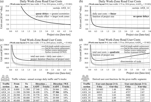
The additional work-zone user costs for the whole project are obtained by multiplying daily user costs by treatment duration in days. Thus, the total (project) user costs are a quadratic function of the project’s size as both daily user costs and project duration are a linear function of the project’s size. In the case of queue formation (layout 2 + 1), the total user costs exhibit economies-of-scale characteristics (Figure 8(c)). If the demand does not exceed the available capacity (layout 3 + 1), the total user costs are lower by an order of magnitude (see Figure 8(d); note the different scale of the y-axis). However, with the increase of project size (>1.0 km), diseconomies of scale occur. The reason for this is that the daily costs converge to a constant value for work zones larger than 1.0 km, while the project duration increases further. In other words, for work-zone lengths which exceed an optimal value (e.g. 1.0 km), it will be more beneficial to have more work zones with shorter durations than to have fewer work zones with longer durations.

In this work, the network-level pavement management is represented by a single freeway or a route (50 lane-km). For a network-wide extension, a network model (e.g. graph) will be needed, taking into account possible detours and the redistribution of traffic demand.

4. Solution methodology

This section describes a new formulation of the M&R optimisation problem based on short survey sections and multiple distress types. The solution is obtained in multiple stages: section-level, work-zone and budget. However, the results from a previous stage are not binding and are only used as initial values, subject to change.

4.1. Section-level optimisation

At the section level, the M&R optimisation problem consists of finding the temporal sequence of treatments (timing and type) that minimises the discounted total agency life-cycle costs over a sufficiently long planning period. In general, there are two principal approaches for determining treatment timing on a single section: threshold-based and/or consideration of user costs. As discussed in Section 3.7, this work does not consider condition-related user costs as their effect within the considered condition thresholds remains limited.

Condition thresholds are employed by many authors as a simplification in the optimisation (e.g. Chu and Chen 2012, Sathaye and Madanat 2012). Although the proposed approach also relies on thresholds at the section level, thresholds are only used as an upper limit for the optimisation of work zones (see Section 4.2). Nevertheless, condition thresholds limit the solution space, with the final solution being optimal only within these limits. This underlines the importance of thresholds in general and their influence on service lives and costs. Furthermore, the fixed thresholds can be relaxed for some distress types (e.g. cracking) if the treatment effectiveness is estimated as a function of the current condition.

The methodology for M&R optimisation at the section level is illustrated in Figure 9. For simplicity, the figure only shows two distress types and the first two treatment applications. As a reminder, service life defines the latest possible timing of treatment application (hard constraint), and at the end of the remaining life a treatment is triggered. The remaining life function equals service life at the time of construction/treatment and decreases linear to zero at the time of failure. For example, in Figure 9, the first failure occurs at t₁ due to surface defects. Alternative 1 includes a surface treatment which delays alligator cracking propagation, but a structural (second) treatment is still needed at time t₂. Alternative 2 consists of bringing forward the structural treatment to the time t₁ resetting both distress types. Depending on the discount rate, if the increase of present value of structural treatment (t₂→t₁) is less than the present value of surface treatment, then the second alternative will be optimal. Although the first distress type that reaches its threshold defines the timing of the first treatment, the type of the selected treatment in the algorithm depends on the effect of the treatment on all distress types and the resulting timing for the second and all subsequent treatments.

Figure 9. Methodology for M&R optimisation on a single road section for multiple distress types based on average costs, condition thresholds and treatment applicability considerations.

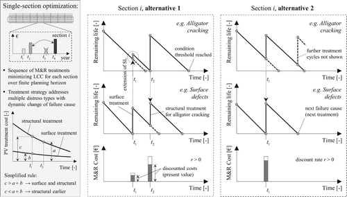
This approach considers all feasible temporal sequences of M&R treatments. In contrast, most models assume repetitive applications of the same treatment or treatment sequence and constant treatment intervals. Furthermore, the selection of a specific treatment determines the failure cause for the next treatment depending on the generated stochastic treatment lives. Thus, failure causes are not known a priori, and the applicability constraints (see Section 3.3) are not fixed but change dynamically during the optimisation.

In this paper, the planning horizon for M&R activities is set to 100 years accounting for residual value at the end of this period. The residual value is computed as a ratio of remaining life to service life of the last planned treatment multiplied by the cost of this treatment (Stone 2013). This value is discounted and subtracted from the total life-cycle costs. In contrast, having a short planning period without accounting for residual value will push the more cost-intensive (structural) repairs right after the end of the period, creating an M&R backlog. As the computation of residual value (with no real market) is somewhat subjective, a combination of long planning period and residual value is preferred. Moreover, a planning horizon of 100 years is adequate with regard to cross-asset optimisation and typical service lives of bridges and tunnels (80–100 years).

The optimisation at the section level uses average treatment costs (without traffic control) and no economies-of-scale cost functions, as the costs would be too high for 50-m sections. This is not a drawback, as both timing and treatment type could be changed at the next stage (work zones). Nevertheless, the single-section optimisation is still needed to optimise the full sequence of treatments up to 100 years. Then, at the second stage, the first three treatments are optimised with regard to work zones, and the remaining sequence of treatments is adopted from the first stage (section level).

4.2. Work-zone optimisation

The work-zone optimisation for short survey sections is, in essence, the main step that distinguishes the proposed methodology from any other approach known to the authors. In contrast to the literature, the focus is not only on operational aspects and short-term impacts of work zones on the road users. Instead, treatment type and timing on short survey sections (50 m) are optimised and coordinated in order to build larger work zones, based on economies-of-scale cost functions (treatment and traffic control costs) and a full life cycle. At the same time, the pavement condition is modelled by using multiple distress types. The present distress or distress combination determines the technical applicability of treatments. Thus, the length and location of a work zone is a pure economic decision, which is based on more accurate predictions with detailed untransformed survey data. The objective for the work-zone optimisation is to minimise the sum of discounted total costs for all considered single sections. The decision variables consist of treatment timing and type with initial (and feasible) values provided by the single-section optimisation.

The proposed approach can only allow the formation of a work zone if the constraints on all involved single sections remain satisfied. Thus, the section with the earliest failure time in a work zone determines the treatment timing for the entire work zone (due to condition thresholds). If failure causes are also different, the treatment selection is based on the most severe (deeper) failure cause (applicability constraint). The methodology for work-zone optimisation is illustrated in Figure 10. For simplicity, only two road sections and one distress type are shown. The treatment on section i corresponds to Alternative 2 in Figure 9. The contiguous section i + 1 has the same first treatment, but at a later time (t₁′). The cost for two separate work zones simply represents the sum of the discounted total costs for both sections. In the case of a combined work zone, both sections share the fixed costs, resulting in lower treatment costs per section. The treatment on section i + 1 is brought forward in this case, resulting in an increased present value and a loss of service life. The optimal alternative is the one with a lower present value of life-cycle costs for both road sections.

Figure 10. Methodology for optimisation of M&R treatment type, timing and work zones for multiple distress types based on economies-of-scale cost functions, condition thresholds and treatment applicability considerations.

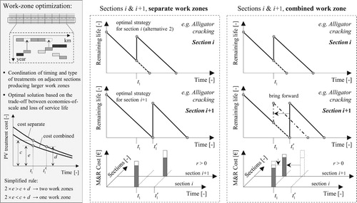
In summary, the work-zone optimisation is based on the trade-off between loss of service life and benefits gained by scale economies. The loss of service life is expressed in monetary terms as the increased present value of the required treatment’s cost. The increase of present value is calculated for all subsequent treatments in the life cycle, as not only the first treatment, but the entire cycle is brought forward. The average work-zone length depends on the degree of spatial correlation (see Section 3.2), the share of fixed costs on total treatment costs and the discount rate. Furthermore, at this stage, work-zone related user costs may be considered as well (see Section 5.4).

4.3. Soft constraints and treatment of outliers

In contrast to long homogeneous sections the proposed model guarantees the satisfaction of all condition thresholds. However, when grouping a number of road sections together, the timing of treatments in resulting work zones equals the timing of the most short-lived section. This may lead to early treatments and an inefficient use of pavement service lives. If the goal is to always satisfy existing condition thresholds, either higher investments will be needed or the agency may choose to adjust these thresholds. In contrast, the current practice is to form long homogeneous sections representing the condition with an average value, which effectively masks current and future condition threshold violations.

A possible way to solve this issue is to model condition thresholds as soft constraints. Thus, the model will allow for the exceedance of thresholds by a specific amount which is determined by a penalty function. For each distress type, one of the two options (hard or soft constraints) has to be chosen. It is reasonable to select hard constraints for distress types related to road safety (e.g. skid resistance, rutting). Soft constraints can be used for other distress types, where the threshold is more arbitrary (e.g. alligator cracking). The use of soft constraints, however, imposes the integration of a performance model which measures the extent of exceedance. The penalty function adds additional costs to the treatment costs, depending on the degree of exceedance. For a road section with more gradual condition deterioration a longer treatment delay will thus be allowed, ceteris paribus, in comparison to a section showing a more rapid deterioration. The penalty cost may be thought of as the additional cost for small repairs maintaining the condition until the timing of the delayed repair is optimal. Alternatively, penalty values may represent condition-related effects from deferring treatments (e.g. water ingress → deeper damage) which are requiring the replacement of more material. In any case, the penalty function must be calibrated in such a way that a postponement of treatments will lead to longer work zones. A first application of this concept is demonstrated in Section 5.2.

Even if soft constraints are used, some sections are not grouped after the optimisation, because it is more economical to pay high fixed costs for a single section then to form a combined work zone. The presence of such outliers (short-lived or long-lived) is not a problem, since these sections could be repaired locally in short-term (daytime) work zones, as long as their number remains limited.

4.4. Complexity and solution approach

A more detailed and accurate modelling (short sections, multiple distress types and treatments) leads to an optimisation problem that is more difficult to solve compared to common approaches. At the section level the number of solutions is limited by applicability and threshold constraints, which allows for an exact solution to be found. An exhaustive search algorithm is automated to perform optimisation for all sections in a sequence. However, the problem of the work-zone optimisation is far more complex (see Figure 11). The decision variables include the type (x_i) and timing (y_i) of treatment on section i. In the literature (e.g. Lee and Madanat 2015), timing is often considered a discrete variable with step size of one year, regardless of the use of a continuous or discrete time deterioration model. In this paper, timing is also an integer. If continuous time is used instead, the solution needs to be rounded to an integer anyway in order for scale economies to apply. Treatment type is also a general integer variable with a domain of possible values {1, 2, 3, 4}.

Figure 11. Size, characteristics and complexity of the formulated optimisation problem. Simple example with 10 sections and evaluation of the objective function for just one decision variable (timing for section 6) and for two decision variables (sections 5 and 6).

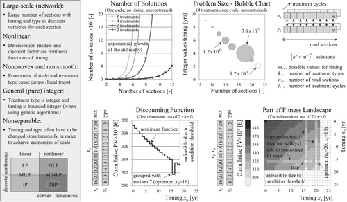
Furthermore, the problem is non-linear as the discounting function and the deterioration models (in general) are not linear. However, the most unpleasant feature of the problem is the non-convex and non-smooth objective function, resulting from economies-of-scale effects and the nominal scale of the treatment type variable. This is another reason why continuous time and mixed-integer formulation are not beneficial, since methods for mixed integer non-linear programming (e.g. outer approximation, generalised Benders decomposition) are suited for solving convex problems.

Thus, an evaluation of the objective function (fitness) landscape for only two variables (timing of sections 5 and 6) sheds light on the complexity of the search space (Figure 11, bottom right). The structure of the real multi-dimensional fitness landscape includes multiple local traps and is difficult to exploit, as there is no specific direction in which the function is increasing or decreasing. Furthermore, the number of possible solutions grows exponentially with the size of the problem (see bubble chart). So, even a relatively small number of road sections (20–30) results in an astronomical number of solutions. Due to the fact that the problem cannot be solved by exact methods, a heuristic method based on stochastic principles is chosen and applied.

The main emphasis of this paper is on the development of a holistic methodology for M&R optimisation, as even the best solution algorithm will be of little use with a poorly developed methodology. Nevertheless, it is important that the formulated problem is tractable and that high-quality solutions can be found within a reasonable time. The results presented in the following section are obtained by making use of a unique algorithm which is tailored to fit the problem at hand. The algorithm is currently being improved, and it will be described in a separate paper due to its complexity. However, some details are already discussed below.

The developed algorithm, currently labelled ‘expand, merge & solve’ (EMS), is based on multiple iterations and resembles features of ‘divide and conquer’ and greedy algorithms (Cormen et al. 2009). Despite the incorporation of a divide and conquer technique, the solution quality is not affected by the decomposition (overlapping is not needed). Thus, EMS is capable of handling an unlimited number of sections, with the running time being proportional to the number of sections. The algorithm code is written using the Visual Basic for Applications (VBA) programming language. For the ‘solve’ part, the commercial software @Evolver 7.5.1, an add-in for Microsoft Excel, is used (Palisade 2015). Evolver’s genetic algorithm is integrated in the EMS algorithm (VBA) using Evolver’s Excel Developer Kit (XDK).

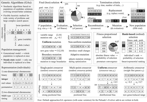
Genetic algorithms (GAs) constitute a metaheuristic search method which is based on the principles of ‘natural selection’ and ‘survival of the fittest’ (Goldberg 1989, Eiben and Smith 2015). GAs are applied in many research areas to solve difficult optimisation problems with complex search spaces. A general overview of GAs is provided in Figure 12. The idea behind GAs is to initially generate and then iteratively enhance a population of solutions with the help of variation (crossover, mutation) and selection (parents, survivor) operators. Eventually, a near-optimal solution will be obtained by examining a relatively small number of possible solutions. Evolver employs an integer representation of solutions, a steady-state population management model, rank-based selection and multiple crossover and mutation operators (see Figure 12). Population size, crossover and mutation rate, as well as stopping time for the algorithm are estimated on the basis of comparative studies. The analysis showed, however, that different combinations of parameters may achieve similar results. Thus, as optimal parameters also depend on the data sample, the importance of parameter tuning should not be overestimated.

Figure 12. General overview of genetic algorithms: simplified example of steady-state GA, as well as most common operators for mutation, parent selection and crossover.

5. Application and results

This section presents the results derived from the application of the proposed methodology (Section 4) to the case study (Section 3.2), with an emphasis on graphical representation which is more suitable for the discussion of the findings on optimal work zones.

5.1. Section-level results

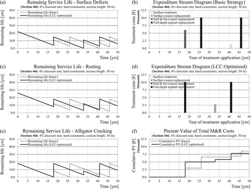
The single-section optimisation is conducted for all 1000 road sections. A (real) discount rate of 4% is used as a standard case (Stone 2013). Figure 13(a,c,e) shows the remaining service life with regard to the three distress types before (basic) and after the optimisation for a randomly chosen section (section 466). The basic (generic) strategy results from selecting the cheapest feasible treatment for the given failure cause. For example, if the failure cause is rutting, the basic strategy will be to select a surface course replacement. The expenditure stream diagrams (Figure 13(b,d)) show that – as a result from life cycle optimisation – three treatments (instead of four) are necessary in the first 50 years, decreasing the associated present value by 9%, as shown in Figure 13(f). Summed up for all 1000 sections, the total reduction of discounted agency costs amounts to 2% (3% undiscounted). Many PMSs, however, do not jointly optimise maintenance, rehabilitation and reconstruction activities and do not consider different temporal treatment sequences. Compared to such strategies, like, for example, ‘treatment 3 only’ (surf & bin course) and ‘treatment 4 only’ (full-depth asphalt), the LCC-optimised strategy results in a total reduction in present value of 9% and 18%, respectively (12% and 17% undiscounted).

Figure 13. Results of the optimisation for a single road section (randomly chosen) with remaining life (a,c,e), expenditure stream (b,d) and present value (f) prior (basic) and after the optimization.

5.2. Work-zone optimisation

The results from the single-section optimisation for 60 contiguous road sections (chosen at random) are shown in Figure 14(a). For simplicity, only the first treatment in the planning period is shown, depicting the positive autocorrelation pattern of service lives. For each section treatment timing is the latest possible. However, such an M&R strategy is not practical due to the excessive number of work zones. For the formation of work zones, scale-economies cost functions must be employed. Minimising the total discounted costs for all sections based on M&R treatment costs generates the work zones shown in Figure 14(b). Significantly larger work zones are obtained from the optimisation when traffic control costs are taken into account according to Figure 14(c). For each work zone, treatment type, timing, work-zone length, layout, duration and costs are computed, together with more a detailed cost calculation and workflow schedule. Despite the fact that, at this point, some work zones already exhibit practical lengths, there is still potential for improvement. For example, a work zone consisting of sections 351–362 may be economically beneficial. The consideration of such an alternative in the optimisation process is not possible due to the condition thresholds. Further investigations show that only a few sections limit the timing of the obtained work zones. For example, the threshold on section 370 is solely responsible for determining the timing (14th year) of the corresponding work zone. Given the subjective nature of condition thresholds, this is a major limitation in any optimisation method.

Figure 14. Results of the work-zone optimization for a segment of 60 road sections (randomly chosen) and 4% discount rate displaying only the first treatment of the life cycle for the cases of no optimization (a), minimum M&R costs (b), minimum total agency costs (c) and minimum total agency costs with soft constraints for alligator cracking (d).

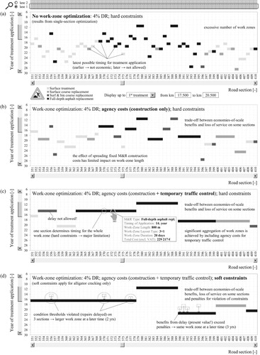
A possible solution to this problem is to model condition thresholds as soft constraints instead of hard constraints (see Section 4.3), with the results shown in Figure 14(d). This approach leads to larger work zones, a better utilisation of service life and longer treatment intervals. In this case, only the threshold for alligator cracking is modelled as a soft constraint. On a general note, in some cases the monetary difference between two separate work zones and one joint work zone is very small (a few euros), so it might be practical to include a small cost tolerance in favour of larger work zones, also benefitting road users.

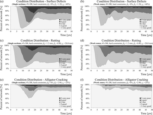
The soft-constraint method requires a penalty function, with penalty costs being added to the objective function (agency costs), taking the amount of threshold violation as a basis. Performance models are needed for estimating threshold violation. Although only alligator cracking is modelled as a soft constraint in the case study, power performance functions (β₀ + β₁ × $\text{S}{\text{L}}^{{\text{β}}_2}$ = y_f) are defined for all distress types. The power parameter implies slightly progressive deterioration (β₂ = 1.20) for surface defects, degressive deterioration (β₂ = 0.80) for rutting and progressive development (β₂ = 2.90) for alligator cracking. The values are taken from previous research (Donev and Hoffmann 2017a), having no impact on the results presented here (except in the case of soft constraints for alligator cracking). Figure 15(a,c,e) shows the condition distribution at the network level (1000 sections) for the three distress types without optimisation of the work zone (see Figure 14(a)). Figure 15(b,d,f) shows the corresponding distributions after the optimisation of work zones (the case of Figure 14(c)). Since both cases employ hard constraints, there is no road section in condition class 5 (very poor). Moreover, the network is in a better average condition as a result of the work-zone optimisation and brought-forward treatments. This secondary effect is more noticeable for the primary and secondary failure cause (alligator cracking and surface defects). At the section level, brought-forward M&R increase the probability of surviving until the treatment timing.

Figure 15. Distress-specific condition distributions for all sections in the cases of no-work zone optimization (a,c,e) and optimal work zones (b,d,f) using power functions to compute intermediate conditions.

5.3. Sensitivity to different discount rates

In the following, the sensitivity of the results should be investigated on the basis of discount rates of 1% and 7%, as presented in Figure 16(a,b), respectively. The results show that lower discount rates lead to greater work-zone lengths. As already mentioned, the work-zone optimisation is based on the trade-off between loss of service life (increase of present value) and economies-of-scale benefits. For the discount rate of 7%, the increase of present value is high, but only for the first treatment, as subsequent treatments show almost no present-value contribution. In the case of 1% discount rate, the increase of present value is not as high, but a greater number or follow-up treatments exhibit a significant increase. In total, the increase of present value for both cases (1% and 7%) is similar. The difference results from discounting the benefit of scale economies. This benefit has much higher present value with lower rates (1%) leading to a greater length of work zones.

Figure 16. Effect of lower (a) and higher (b) than 4% discount rates on optimal work zones, treatment types and timings for the case of minimum total agency costs and hard constraints.

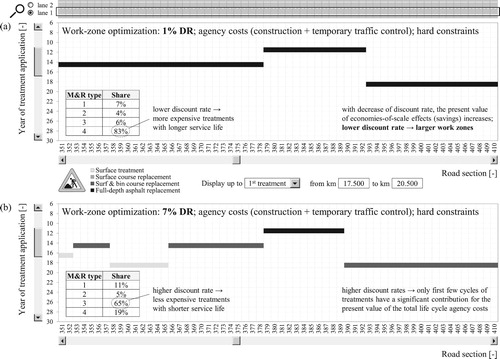
In addition to the length of the work zone, the applied discount rate shows a major impact on the type of the treatment. For example, a higher discount rate leads to preference of partial-depth replacement (treatment 3) over full-depth replacement (treatment 4). High discount rates attach more importance to short-term decisions favouring less costly treatments, despite the shorter service lives. On the other hand, given that future pavement performance and associated treatment costs are largely uncertain, low discount rates (implying a high level of certainty for the type and timing of future treatments) are not very appropriate.

The number of work zones by length and treatment type for all 1000 road sections is presented in Figure 17. Neglecting traffic control costs results in average work zones of 120 m, as shown in Figure 17(e). The average length of a work zone increases with the decrease of discount rates. The greatest average work-zone length (575 m) is achieved in the case of soft constraints (Figure 17(d)). Short work zones (<200 m) mainly include surface treatments which are applied as short-term work zones and may not be representative for the average work zone. In some cases, work zones of up to 4000 m are proposed.

Figure 17. Number of work zones in different length classes by type of treatment for cases of different discount rates (a,b,c), soft constraints (d) and minimum M&R costs (e).

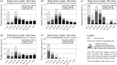
The average length of a work zone may seem too short as compared to typical lengths known from practice. On the one hand, there is no proof that the work zones in practice are optimal from an economic point of view. On the other hand, the optimisation does not yet account for a few factors that will significantly increase the obtained work-zone lengths. First, an aggregated work zone may include multiple M&R activities (see Figure 14(c), sections 390–408). These sections may share the fixed costs for traffic control and part of the fixed costs for construction. Two work zones with a small gap in between (i.e. sections where no construction activities take place, but the same traffic control applies) can also be aggregated in one joint work zone. For this purpose, some additional constraints reflecting the approach in practice have to be defined (e.g. technically reasonable activity combinations, maximum gap length, maximal number of different activities, etc.). These situations are currently not considered, but the model can easily be adjusted to account for them.

Second, the employed cost models currently consider fixed costs related to construction and temporary traffic control. Other (in-house) activities with a high proportion of fixed costs are not included yet (e.g. costs for supervision and planning, road safety audits, carrying out of call-for-tender procedures, quality assurance and acceptance testing). Taking into account these costs will further reduce the number of work zones and increase their length. On the other hand, considering the second roadway lane will lead to a shorter average work-zone length (due to economies-of-scale in transverse direction). With less than 5% of the truck traffic on the interior lane in Austria, however, it is to be expected that the interior lane will require substantially less frequent structural repairs.

5.4. Selection of a work-zone layout

In the following, additional road user costs which are caused by work zones should be considered. The corresponding objective is to minimise the sum of agency (including traffic control) and user costs. The optimisation is conducted for two work-zone layouts: 2 + 1 and 3 + 1, as shown in Figure 18(a,b). The results are proof that the taking into account of user costs leads, in general, to larger work zones. For the given traffic section (AXX_14), the available capacity of layout 2 + 1 is not sufficient to accommodate the traffic demand, resulting in a queue and very high user costs. In contrast, the configuration 3 + 1 does not cause congestion and leads to user costs which are approximately nine times lower (60 sections). However, maintaining the number of open lanes by using median crossover leads to higher agency costs (20%). In the case of 2 + 1, the forced-flow conditions lead to much higher user costs, resulting in a higher level of aggregation (only two work zones) in comparison to 3 + 1.

Figure 18. Effect of considering user costs together with agency costs in the work-zone optimization for layout 2 + 1 (a) and layout 3 + 1 (b) and a given traffic section (AXX_14). Selection of a work-zone layout based on total (agency plus user) costs.

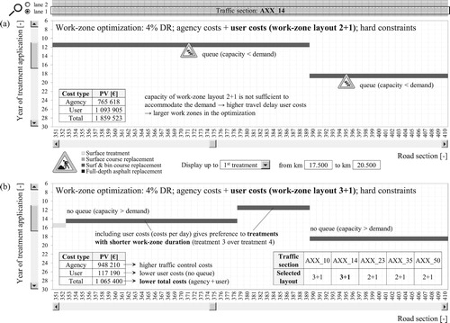
Besides greater work-zone lengths, considering user costs leads to different optimal treatment types (see Figure 14(c) for comparison). Work-zone user costs are computed as the product of daily user costs and project duration. Thus, it is not surprising that treatments with a shorter duration (treatment 3) are preferred over treatments with a longer duration (treatment 4). User costs (non-cash expense) are subjective and primarily represent short-term impacts. Therefore, they should not be mixed with agency costs which are of a more objective nature. Instead, it is recommended to utilise user costs in making short-term decisions (e.g. selection of work-zone configurations). In the present case, layout 3 + 1 will be selected for minimising total costs. The layouts for the other traffic segments are provided in the table of Figure 18(b). Subsequently, work-zone optimisation can be conducted with the determined layouts based solely on the agency costs. By doing so, the interests of road users will be taken into account (even if this adds up to more expensive traffic control), but other decisions with long-term impacts like treatment type and work-zone length will be more stable as they are based on agency costs.

5.5. Special topic: pavement design optimisation

The main idea of long-life (perpetual) pavements is to design thicker pavements in order to avoid premature structural failure (Timm and Newcomb 2006). Such pavements mainly exhibit surface-related distress and require minor (light) rehabilitation which results in lower life cycle costs despite higher initial construction costs. In the context of the case study (with alligator cracking as a dominant failure cause), the effects of extending structural life by thicker design is investigated. For this purpose, the expectation of the service-life distribution for alligator cracking is extended from 19.4 to 24.2 years (by 4.8 years). The service life distributions for surface defects and rutting remain unchanged, as they are not affected by thicker design.

Figure 19(a) shows the optimal work zones minimising agency life cycle costs (including traffic control) for the standard design case (19.4 years). This figure supplements Figure 14(c) by displaying the second and the third treatment, not previously shown, as the focus of the discussion was on work zones. It is also shown that the employed (EMS) algorithm evaluates work zones consisting of, for example, the second treatment (on one section) and the third treatment (on the neighbouring section). Figure 19(c) includes the corresponding work zones with enhanced design (24.2 years). Extending the life for alligator cracking by 4.8 years on average leads to a new dominant (first) failure cause (surface defects with 55%). The first visible consequences based on the segment of 60 sections are an increased share of minor treatments (treatments 1 and 2), as well as shorter work zones and treatment intervals.

Figure 19. Comparison of work zones, annual budget and distribution of treatment types for the standard case of minimum total agency costs, hard constraints and 4% discount rate (a,b) and for the case of enhanced design life for alligator cracking under the same conditions (c,d) with display of the first three treatment cycles.

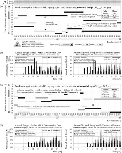
For the entire network (50 lane-km), the annual M&R expenditures and length-dependent treatment type distributions (treatment demand) for both cases of standard and enhanced design are shown in Figure 19(b,d). The annual costs are provided in 2016 constant-value euros (inflation free) and constitute net costs excluding value-added tax (VAT). For simplicity, only the first 30 years are shown, although the planning horizon is 100 years. The comparison of average annual M&R costs (years 6–30) shows that extending design life leads to a reduction in costs from €0.65 million to €0.57 million per year (12% reduction), despite shorter work zones and treatment intervals. The treatment-demand diagrams show that the share of minor treatments is significantly increased in the case of enhanced design. Furthermore, the treatment-demand peak has shifted from years 13–14 to years 17–18, but the total repaired network area is almost the same in both cases.

The difference in annual expenditures and present value is highlighted in Figure 20(a,b). The strategy with extended structural life leads to an M&R cost reduction of €2.08 million over 30 years. The majority of these M&R savings are incurred in the first 15 years, with the enhanced design being more expensive in the second half of the shown period. The total reduction in present value amounts to €1.73 million (4% discount rate). In order to determine whether the enhanced design reduces total life cycle costs or not, the initial construction costs have to be considered. These costs are not taken into account here due to the absence of a reliable empirical model which links pavement thickness and service life. However, for €1.73 million, approximately 7 cm of asphalt base course could be added to the pavement structure (for all 1000 sections). The singular aim of this example is to show that structural design life has a major impact on life-cycle costs, and pavement thickness should therefore be a subject of optimisation. This conclusion is in contrast to the fixed design life of 20 years which is embedded in the standard procedures of many countries, but is in accordance with similar findings in scientific literature (McDonald and Madanat 2012, Lee and Madanat 2014).

Figure 20. Potential savings as a result of avoiding premature structural failures by extending design life for alligator cracking in terms of annual budget (a) and present value (b). Total agency costs including TTCC (c) with histogram of treatment intervals (d) in the standard design case.

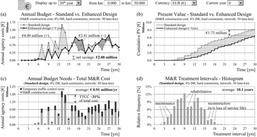
The total agency costs are shown in Figure 20(c), with the costs for temporary traffic control amounting to 31% of total costs. This percentage can be reduced with the ongoing development of the approach and the potential increase of the length of work zones (see Section 5.3). The probability distribution of treatment intervals shows a wide dispersion which is attributed to the different service lives of the employed treatments (see Figure 20(d)), with the average interval being 10.1 years.

If budget constraints are not binding, the solution derived by unconstrained work-zone optimisation is final. The network-level M&R optimisation under annual agency budget constraints will be the subject of a forthcoming paper. The solution of the unconstrained problem, however, is the best possible solution for the agency. Any other M&R programme resulting from budgetary restrictions is suboptimal, assuming that condition thresholds are not violated.

6. Conclusions

The primary goal of any PMS is to determine optimal M&R strategies for each section of a road network, subject to an annual budget. State-of-the-art PMS aggregate short survey sections into longer homogeneous sections, prior to any optimisation. Due to averaging effects, the estimated service lives are not accurate, condition thresholds are systematically violated and a determination of optimal work zones is no longer possible. Instead of forming long homogeneous sections, the proposed approach is based on short survey sections, allowing for more accurate condition predictions for each failure type and stricter threshold control. Survey sections are combined into longer work zones based on economies-of-scale effects, optimising agency M&R and TTCCs. In addition, work-zone related user and environmental costs are taken into account in order to select appropriate work-zone layouts.

Common approaches are based on a single condition index which represents pavement condition and on predefined M&R strategies (temporal sequence of treatment types). In contrast, the suggested method considers every possible sequence of treatments, depending on the predicted distress types or a combination thereof. The proposed approach is unique in its capabilities to simultaneously account for multiple treatments, multiple distress types, stochastic treatment lives, scale economies, traffic control, work-zone layouts, capacity and road user impacts. The developed cost and performance models are an integral part of the optimisation approach. All input information is estimated on the basis of real data or an extensive literature comparison and calibrated for flexible pavements on freeways in Austria. The formulated optimisation problem exhibits exponential complexity and is solved by a unique algorithm which is specifically designed for this class of problems.

The proposed methodology is successfully applied to a case study with a realistic road network consisting of 1000 consecutive sections. The results show the superiority of the proposed approach when compared to a predefined sequence of treatments at the single section level. According to the results, traffic control costs are the primary driver for the formation of work zones. The use of soft constraints increases the flexibility of the approach, reducing the dependence of the results on condition thresholds and outliers. Furthermore, the conducted sensitivity analysis shows that discount rates have a huge impact on the length of work zones and the type of the treatment. Higher discount rates attach more weight to short-term decisions and favour less costly treatments, despite shorter service lives. The consideration of additional user costs due to work zones leads to larger work zones and treatments with a shorter duration. In the light of the European Commission’s strategy towards internalisation of transport accident and environmental costs, the model is capable of addressing these challenges, providing the means for an estimation of future infrastructure charges.

Furthermore, the designed structural life has a huge impact on the extent of subsequent treatments and life cycle costs. Extended-life pavements have the potential to reduce total agency costs and road user impacts with less costly surface treatments, shorter work zone durations and a reduction of lane closures, especially in the case of low discount rates. Future developments include the extension of the model to simultaneous modelling of multiple lanes, estimation of optimal inspection intervals, application to rigid pavements and cross-asset optimisation. A follow-up paper that is currently under preparation will compare the developed holistic model framework and methodology to existing PMS approaches, with and without budget constraints, based on the presented case study.

Acknowledgement

The authors acknowledge the TU Wien University Library for financial support through its Open Access Funding Programme.

Disclosure statement

No potential conflict of interest was reported by the authors.

ORCID

Valentin Donev http://orcid.org/0000-0002-3933-971X

References

- AASHTO, 2012. Pavement management guide. 2nd ed. Washington, DC: American Association of State Highway and Transportation Officials.
- Anastasopoulos, P.C., et al., 2012. Empirical assessment of the likelihood and duration of highway project time delays. Journal of Construction Engineering and Management, 138 (3), 390–398. doi: 10.1061/(ASCE)CO.1943-7862.0000437
- Anastasopoulos, P.C. and Mannering, F.L., 2015. Analysis of pavement overlay and replacement performance using random parameters hazard-based duration models. Journal of Infrastructure Systems, 21 (1), 04014024. doi: 10.1061/(ASCE)IS.1943-555X.0000208
- Bennett, C.R. and Greenwood, I.D., 2001. Modeling road user and environmental effects in HDM-4. Highway development and management series, vol. 7. Paris: World Road Association (PIARC).
- Birbaum, J., 2016. Entwicklung eines Verfahrens zur Ermittlung der Lebenszykluskosten von Straßen in Asphaltbauweise [Development of a procedure to determine the life-cycle-costs of asphalt roads]. Dissertation (PhD). Universität Siegen (in German).
- BMVIT, 2013. Transport in figures: Austria – edition 2011. Vienna: Federal Ministry for Transport, Innovation and Technology (BMVIT).
- Brozek, B., Litzka, J., and Weninger-Vycudil, A., 2009. Entwicklung eines nutzerkostenmoduls im österreichischen PMS [Development of a user cost module in the Austrian pavement management system]. Wien: BMVIT, Straßenforschung Heft 585 (in German).
- Chen, C.H. and Schonfeld, P., 2007. Pavement resurfacing intervals in work zone optimization. 86th annual meeting of the Transportation Research Board, 21–25 January, Washington, DC.
- Chien, S. and Schonfeld, P., 2001. Optimal work zone lengths for four-lane highways. Journal of Transportation Engineering, 127 (2), 124–131. doi: 10.1061/(ASCE)0733-947X(2001)127:2(124)
- Chu, J.C. and Chen, Y.-J., 2012. Optimal threshold-based network-level transportation infrastructure life-cycle management with heterogeneous maintenance actions. Transportation Research Part B, 46 (9), 1123–1143. doi: 10.1016/j.trb.2012.05.002
- Cormen, T.H., et al., 2009. Introduction to algorithms. 3rd ed.Cambridge, МА: MIT Press.
- Cuelho, E., Mokwa, R., and Akin, M., 2006. Preventive maintenance treatments of flexible pavements: a synthesis of highway practice. Report no. FHWA/MT-06-009/8117-26. Helena, MT: Montana Department of Transportation.
- Donev, V., and Hoffmann, M., 2017a. Condition prediction and estimation of service life in the presence of data censoring and dependent competing risks. International Journal of Pavement Engineering. doi.10.1080/10298436.2017.1293264.
- Donev, V., and Hoffmann, M., 2017b. Network-level optimization of pavement M&R activities, timing and work-zone length for multiple distress types. World Conference on Pavement and Asset Management, 12–16 June, Milan, Italy.
- Eiben, A.E. and Smith, J.E., 2015. Introduction to evolutionary computing. 2nd ed.Berlin: Springer.
- Ferreira, A., Picado-Santos, L., and Antunes, A., 2002. A segment-linked optimization model for deterministic pavement management systems. International Journal of Pavement Engineering, 3 (2), 95–105. doi: 10.1080/10298430290030603
- Fischer, L., 2009. Wirtschaftlichkeitsuntersuchung von Behelfsverkehrsführungen an Autobahnarbeitsstellen unter Berücksichtigung der Querschnittsabmessungen [Economic feasbility study of work-zone layout types and traffic control on freeways with regard to the dimensions of the cross section]. Bauhaus-Universität Weimar (in German).
- Frommet al., 2012. ASFINAG: erhaltungsstrategie [ASFINAG: asset management strategy]. Wien: ASFINAG Service GmbH und ASFINAG Alpenstraßen (unpublished, in German).
- FSV, 2010. RVS 02.01.22: nutzen-kosten-untersuchungen im verkehrswesen [Transportation cost and benefit analysis]. Wien: Forschungsgesellschaft Straße-Schiene-Verkehr (in German).
- FSV, 2012. RVS 05.05.42: straßen mit getrennten richtungsfahrbahnen [Roads with separate directional carriageway]. Wien: Forschungsgesellschaft Straße-Schiene-Verkehr (in German).
- FSV, 2016. RVS 03.08.63: oberbaubemessung [Pavement design]. Wien: Forschungsgesellschaft Straße-Schiene-Verkehr (in German).
- Fwa, T.F., Chan, W.T., and Tan, C.Y., 1996. Genetic-algorithm programming of road maintenance and rehabilitation. Journal of Transportation Engineering, 122 (3), 246–253. doi: 10.1061/(ASCE)0733-947X(1996)122:3(246)
- Goldberg, D.E., 1989. Genetic algorithms in search, optimization & machine learning. Reading, MA: Addison-Wesley.
- Haas, R., Hudson, W.R., and Zaniewski, J., 1994. Modern pavement management. Malabar, FL: Krieger.
- Hajdin, R. and Lindenmann, H.-P., 2007. Algorithm for the planning of optimum highway work zones. Journal of Infrastructure Systems, 13 (3), 202–214. doi: 10.1061/(ASCE)1076-0342(2007)13:3(202)
- Hall, K.T., et al., 2001. Rehabilitation strategies for highway pavements. NCHRP Project C1-38: Conctractor’s final report. Washington, DC: Transportation Research Board.
- Hamilton, J.D., 1994. Time series analysis. Princeton, NJ: Princeton University Press.
- Hellmann, L., Rübensam, J., and Schwiethal, S., 2008. Entwicklung von verfahrenshilfen zur berücksichtigung baustellenbedingter nutzerkosten im erhaltungsmanagement [Development of process procedures in the maintenance management, considering construction site-specific user costs]. Bonn: Forschung Straßenbau und Straßenverkehrstechnik, Heft 988 (in German).
- Hoffmann, M., and Donev, V., 2017. Optimization of pavement M&R activities and work zones with user costs for multiple distress types. World Conference on Pavement and Asset Management, 12-16 June, Milan, Italy.
- Jiang, X. and Adeli, H., 2003. Freeway work zone traffic delay and cost optimization model. Journal of Transportation Engineering, 129 (3), 230–241. doi: 10.1061/(ASCE)0733-947X(2003)129:3(230)
- Kuhn, K.D. and Madanat, S.M., 2005. Model uncertainty and management of a system of infrastructure facilities. Transportation Research Part C, 13 (5), 391–404. doi: 10.1016/j.trc.2006.02.001
- Lea, J.D. and Harvey, J.T., 2015. Using spatial statistics to characterise pavement properties. International Journal of Pavement Engineering, 16 (3), 239–255. doi: 10.1080/10298436.2014.942856
- Lee, J. and Madanat, S., 2014. Joint optimization of pavement design, resurfacing and maintenance strategies with history-dependent deterioration models. Transportation Research Part B, 68, 141–153. doi: 10.1016/j.trb.2014.06.008
- Lee, J. and Madanat, S., 2015. A joint bottom-up solution methodology for system-level pavement rehabilitation and reconstruction. Transportation Research Part B, 78, 106–122. doi: 10.1016/j.trb.2015.05.001
- Lindenmann, H.P., 2008. Massnahmenplanung im erhaltungsmanagement von fahrbahnen; synthesebericht [Action planning within the management of road maintenance; synthesis report]. UVEK-schriftenreihe Nr. 1259. Zürich: Schweizerischer Verband der Strassen- und Verkehrsfachleute (in German).
- Mallela, J. and Sadasivam, S., 2011. Work zone road user costs: concepts and applications. Report no. FHWA-HOP-12-005. Washington, DC: Federal Highway Administration.
- McDonald, M. and Madanat, S., 2012. Life-cycle cost minimization and sensitivity analysis for mechanistic-empiric pavement design. Journal of Transportation Engineering, 138 (6), 706–713. doi: 10.1061/(ASCE)TE.1943-5436.0000346
- Medury, A. and Madanat, S., 2013. Incorporating network considerations into pavement management systems: a case for approximate dynamic programming. Transportation Research Part C, 33, 134–150. doi: 10.1016/j.trc.2013.03.003
- Meissner, G., 2014. Correlation risk modeling and management: an applied guide including the basel III correlation framework – with interactive correlation models in excel/VBA. 1st ed.Singapore: Wiley.
- Montgomery, D.C., Jennings, C.L., and Kulahci, M., 2015. Introduction to time series analysis and forecasting. 2nd ed.Hoboken, NJ: Wiley.
- Nobakht, M., et al., 2016. Mechanistic-empirical methodology for the selection of cost-effective rehabilitation strategy for flexible pavements. International Journal of Pavement Engineering. doi./10.1080/10298436.2016.1199878.
- Ntziachristos, L. and Samaras, Z., 2016. Exhaust emissions from road transport. In: EMEP/EEA air pollutant emission inventory guidebook 2016. EEA Report no. 21/2016. Luxembourg: European Environment Agency.
- Ogwang, A., 2016. Threshold-based resurfacing policies in pavement management to minimize costs and greenhouse gas emissions. Dissertation (PhD). University of California, Berkeley.
- Palisade, 2015. Evolver: the genetic algorithm solver for Microsoft Excel. User’s guide, version 7. Ithaca, NY: Palisade.
- Rossetti, M.D., 2016. Simulation modeling and arena. 2nd ed.Hoboken, NJ: Wiley.
- Santos, J., Ferreira, A., and Flintsch, G., 2017. An adaptive hybrid genetic algorithm for pavement management. International Journal of Pavement Engineering. doi.10.1080/10298436.2017.1293260.
- Sathaye, N. and Madanat, S., 2012. A bottom-up optimal pavement resurfacing solution approach for large-scale networks. Transportation Research Part B, 46 (4), 520–528. doi: 10.1016/j.trb.2011.12.001
- Stone, M.L.C., 2013. Development of unit cost estimating models with respect to scale economies and material price volatility for use in probabilistic life cycle cost analysis. Dissertation (PhD). University of Alabama.
- Timm, D.H. and Newcomb, D.E., 2006. Perpetual pavement design for flexible pavements in the US. International Journal of Pavement Engineering, 7 (2), 111–119. doi: 10.1080/10298430600619182
- Walls III, J. and Smith, M.R., 1998. Life-cycle cost analysis in pavement design: interim technical bulletin. Report no. FHWA-SA-98-079. Washington, DC: Federal Highway Administration.
- Wießmayer, W., 2006. B1 Wiener Straße Teststrecke: Abschlussbericht [B1 Wiener Straße test track: final report]. Linz: Amt der O.ö. Landesregierung – Landesbaudirektion, Abteilung Straßenerhaltung und – betrieb (in German).
- Williams, R.C., Hildreth, J.C., and Vorster, M.C., 2009. Highway construction data collection and treatment in preparation for statistical regression analysis. Journal of Construction Engineering and Management, 135 (12), 1299–1306. doi: 10.1061/(ASCE)CO.1943-7862.0000112
- Wirtgen, 2013. Wirtgen cold milling manual: technology and application. Windhagen, Germany: Wirtgen GmbH.
- Yang, N., 2010. Optimization of highway work zone decisions considering short-term and long-term impacts. Dissertation (PhD). University of Maryland.
- Yeo, H., Yoon, Y., and Madanat, S., 2013. Algorithms for bottom-up maintenance optimisation for heterogeneous infrastructure systems. Structure and Infrastructure Engineering, 9 (4), 317–328. doi: 10.1080/15732479.2012.657649