Effect of stone-on-stone contact on porous asphalt mixes: micromechanical analysis

ABSTRACT

Within the pavement engineering community, porous asphalt (PA) mixes are regarded as mixes capable of reducing noise and improving wet skid resistance. However, these mixes are likely to have the distress of ravelling. In order to analyse the propensity of a given PA mix for ravelling, the homogenisation technique can be considered as an attractive method. Along the line of the homogenisation technique, micromechanical models have been used to predict the stiffness of asphalt mixes. However, it was found that the predicted results were not in good agreement with the experimental values due to the fact that the stiffness of interacted aggregates was not accurately accounted in the models. To deal with this issue, it is important for researchers to study the stiffness of the interacted aggregates network and its role in the behaviour of a given mix. Based on this realisation, this paper provided a methodology to estimate the stiffness of the stone-on-stone skeleton and its role in the overall response of PA mixes. The results showed that the predicted stiffness of the stone-on-stone skeleton is dependent on the loading frequency/temperature and the compaction effort. The frequency response of the stone-on-stone skeleton is similar to that of the mix.

KEYWORDS:

• Porous asphalt mixes (open graded friction course mixture; permeable friction course mixture)
• stone-on-stone skeleton
• micromechanical analysis

Introduction

Porous asphalt (PA) mix (also called open graded friction course mixture or permeable friction course mixture) is a pavement surfacing material with a high air voids content as compared to the commonly used dense asphalt (DA) mix. PA mix is known to have the advantage of improving skid resistance and reducing noise (Hardiman 2004, Mansour and Putman 2013, Srirangam et al. 2015). It is also effective in reducing the splashing and spraying in wet weather to improve the safety of the pavement (Hardiman 2004, Mansour and Putman 2013).

Although there are many advantages of PA mixes, it has been widely reported that these mixes are likely to have the distress of ravelling (Kandhal and Mallick 1988, Mansour and Putman 2013), where aggregate particles are separated from the surface of the pavement. In some cases, ravelling can dominate the failure of the mix and significantly reduce the expected service life of the pavement (Kringos and Scarpas 2008).

Researchers (Mo et al. 2007) have pointed out that insights into ravelling can be obtained by investigating the stress/strain fields of each constituent (phase). This is due to the fact that ravelling is contributed by the cohesive damage which is a failure of binder properties, and the adhesive damage which is a failure of the bond between the binder and aggregate particles (Mo et al. 2007, Kringos and Scarpas 2008).

Over the years, many studies have been conducted to obtain the stress/strain fields of each phase and further analyse the propensity of a given PA mix for ravelling (Kringos and Scarpas 2005, Mo et al. 2007, Kringos and Scarpas 2008, Mo et al. 2009, Ghauch et al. 2015, Manrique-Sanchez et al. 2018). Most of these studies used the computational technique based on the finite element method (FEM)/discrete element method (DEM). Although FEM/DEM based models are able to handle the detailed characteristics of various phases, they require large-scale and sometimes impractical computational facilities (Anupam et al. 2014, Anupam et al. 2016, Anupam et al. 2017).

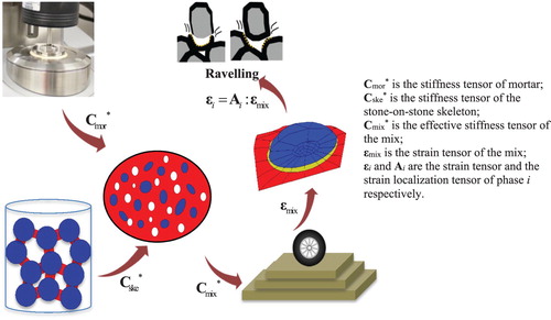
The homogenisation technique can be considered as an attractive alternative to obtain the stress/strain fields of each phase without the need for much computation facilities, see Figure 1. By means of the homogenisation technique, the effective stiffness of the mix is determined from the properties of its different phases. On the basis of the homogenised stiffness, the stress/strain fields of the mix can be calculated by means of pavement analysis tools (Siddharthan et al. 1998, Siddharthan et al. 2000). Lastly, the local stress/strain fields in the individual phases can be calculated by using the homogenisation technique in an inverse way. These local stress/strain fields can be further used to analyse the propensity of a given mix for ravelling by comparing them to the experimental results of the characteristics of the cohesive fatigue damage and adhesive fatigue damage.

Figure 1. The diagram of the homogenisation technique.

Along the line of the homogenisation technique, micromechanical models, i.e. the Mori-Tanaka (MT) model (Mori and Tanaka 1973, Benveniste 1987), the Self-consistent (SC) model (Budiansky 1965, Hill 1965), the Generalised self-consistent (GSC) model (Christensen and Lo 1979), the differential model (Norris 1985), etc. have been evaluated by several research groups (Buttlar 1996, Kim and Little 2004, Lackner et al. 2005, Shu and Huang 2008, Kim and Buttlar 2011, Underwood and Kim 2013) with the objective of predicting the stiffness of asphalt mixes.

However, most of the studies (Shu and Huang 2008, Kim and Buttlar 2011, Underwood and Kim 2014, Zhang et al. 2018a) found that the predicted results were not in good agreement with the experimental values especially at lower frequencies. It was hypothesised by the authors of these works (Buttlar 1996, Buttlar et al. 1999, Kim and Little 2004, Abbas et al. 2005, Underwood and Kim 2014) that this could be associated with the fact that the stiffness of the interacted aggregates was not accurately taken into account.

To deal with the above issue, it is important for researchers to study the stiffness of the interacted aggregates network and its role in the behaviour of a given mix. On the basis of the obtained knowledge, the micromechanical models could be developed and the accuracy of the predictions could be improved. For example, learning about whether the stiffness of the interacted aggregates network is temperature dependent or not could help researchers accurately consider the effect of frequencies on the predictions.

In a PA mix, it is known that an interconnected coarse aggregates network (called as a stone-on-stone skeleton) is formed among a large volume fraction of coarse aggregates (Alvarez et al. 2010, Wang et al. 2016, Chen and Wong 2017, Alvarez et al. 2018, Li et al. 2019). Due to the formation of the stone-on-stone skeleton, the performance of PA mixes, such as the ravelling resistance, the permanent deformation resistance, etc., significantly depends on its material properties. In this case, the study on the stiffness of the stone-on-stone skeleton and its role in the behaviour of PA mixes is even more important for researchers.

With the above realizations, the aim of this paper is to provide a methodology to estimate the stiffness of the stone-on-stone skeleton and its role in the behaviour of PA mixes. The scope of this study includes:

• To propose a way to obtain the stiffness of the stone-on-stone skeleton in PA mixes;

• To discuss the effect of the loading temperature/frequency and the compaction effort on the stiffness of the stone-on-stone skeleton;

• To discuss the role of the stone-on-stone skeleton on the behaviour of PA mixes.

Background

Micromechanical modelling

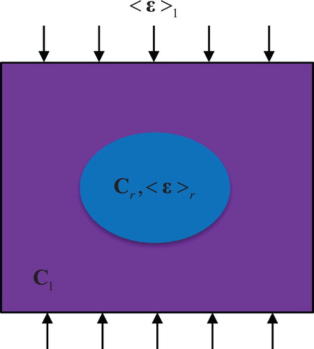
In micromechanical modelling, a material is considered to be composed of a matrix with different inclusions embedded into it. The effective stiffness of the composite C _eff can be related to the properties of the matrix and the inclusions via the following equation:(1) ${\mathbf{C}}_{\mathrm{eff}}=f_1{\mathbf{C}}_1:{\mathbf{A}}_1+\sum _{r=2}^N{f}_r{\mathbf{C}}_r:{\mathbf{A}}_r(1)$(1) where f₁ and C ₁ denote the volume fraction and the stiffness tensor of the matrix; f_r and C_r are the volume fraction and the stiffness tensor of the rth inclusion phase; and A ₁ and A_r are known as the strain localisation tensors, which describe the relationship between the average strains of the matrix and each inclusion phase with the average strain of the overall composite (Ghossein and Lévesque 2014).

Equation (1) shows that the value of C _eff can be obtained from the volume fraction and the stiffness of each phase. However, it can also be seen that once the value of C _eff is known, the stiffness of any phase can be obtained as well. Based on this realisation, a methodology for calculating the stiffness of the stone-on-stone skeleton was proposed.

A proposed methodology to predict the stiffness of the stone-on-stone skeleton

To calculate the stiffness of the stone-on-stone skeleton, any of the micromechanical models (i.e. the MT model, the SC model, the GSC model and the differential model, etc.) can be used. However, the MT model was chosen as the most appropriate one in this study. This is based on the fact that the performance of this model for predicting the stiffness of PA mixes is better than the SC model and the GSC model according to the previous research of the authors (Zhang et al. 2018a). In addition, in comparison to the differential model, the MT model is much easier to be used.

Mori-Tanaka model

In the MT model, inclusions are considered to be embedded into the deformed matrix with an average strain of <ε>₁, see Figure 2. The average strain in each inclusion phase <ε>_r is related to the value of <ε>₁ via Equation (2).(2) $<\epsilon {>}_r={\mathbf{T}}_r:<\epsilon {>}_1,r=2,3,\dots ,N$(2) with(3) ${\mathbf{T}}_r=[\mathbf{I}+{\mathbf{S}}_1:({\mathbf{C}}_1{)}^{-1}:({\mathbf{C}}_r-{\mathbf{C}}_1){]}^{-1}$(3) where I is the fourth-order identity tensor.

Figure 2. Illustration for the MT model.

In Equation (3), S ₁ is known as the Eshelby’s tensor (Eshelby 1957). The value of S ₁ is related to the mechanical and geometrical properties of the matrix and the inclusions. By considering both the matrix and the inclusions as isotropic and the inclusions as spherical, the value of S ₁ can be calculated as follows:(4) ${\mathbf{S}}_1={\alpha }_1{\mathbf{I}}^{\mathrm{v}}+{\beta }_1{\mathbf{I}}^{\mathrm{d}}$(4) with(5) ${\alpha }_1={\displaystyle \frac{3{\kappa }_1}{3{\kappa }_1+4{\mu }_1},{\beta }_1={\displaystyle \frac{6({\kappa }_1+2{\mu }_1)}{5(3{\kappa }_1+4{\mu }_1)}}}$(5) where I _v and I _d denote the volumetric part and deviatoric part of I, respectively; and κ₁ and μ₁ are the bulk modulus and the shear modulus of the matrix, respectively.

On the basis of the well-known relationship between <ε>_r and the average strain of the composite <ε>_c (Equation (6)), Equation (2) can be substituted into Equation (6) to obtain the relationship between <ε>₁ and <ε>_c, see Equation (7).(6) $<\epsilon {>}_{\mathrm{c}}=\sum _{r=1}^N{f}_r<\epsilon {>}_r$(6) (7) $<\epsilon {>}_1={\left(f_1\mathbf{I}+\sum _{r=2}^N{f}_r{\mathbf{T}}_r\right)}^{-1}:<\epsilon {>}_{\mathrm{c}}$(7) From Equation (7), the value of A ₁ for the matrix can be given as:(8) ${\mathbf{A}}_1={\left(f_1\mathbf{I}+\sum _{r=2}^N{f}_r{\mathbf{T}}_r\right)}^{-1}$(8) By substituting Equation (7) into Equation (2), the value of A_r for each inclusion phase can be obtained as:(9) ${\mathbf{A}}_r={\mathbf{T}}_r:{\left(f_1\mathbf{I}+\sum _{j=2}^N{f}_j{\mathbf{T}}_j\right)}^{-1},r=2,3,\dots ,N$(9) The predicted value of C _eff by the MT model can be further obtained by substituting the values of A ₁ and A_r into Equation (1):(10) ${\mathbf{C}}_{\mathrm{eff}}=\left(f_1{\mathbf{C}}_1+\sum _{r=2}^N{f}_r{\mathbf{C}}_r:{\mathbf{T}}_r\right):{\left(f_1\mathbf{I}+\sum _{j=2}^N{f}_j{\mathbf{T}}_j\right)}^{-1}$(10) It is noted here that although the MT model was initially developed for elastic materials, the model can use the elastic-viscoelastic correspondence principle to obtain solutions of the effective mechanical properties of viscoelastic materials (Hashin 1970). Effective complex moduli of a viscoelastic material can simply be obtained by replacing the elastic moduli (Equation (10)) with their equivalent complex moduli.

Procedures for calculating the stiffness of the stone-on-stone skeleton

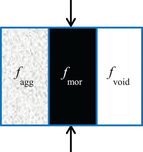
In most of the previous studies (Abbas et al. 2005, Shu and Huang 2009, Underwood and Kim 2013), typically, the mortar (asphalt binder, filler and sand) is regarded as the matrix phase in an asphalt composite. However, this assumption might not be valid for PA mix because in comparison to DA mix, PA mix has a higher air voids content and a lower mortar content, which means that the mortar may not completely interact with each other and form a continuum medium, see Figure 3. Furthermore, since a stone-on-stone skeleton is formed in PA mix, the transfer of the load in the mix should mainly depend on the connected stone particles rather than the mortar. Therefore, in PA mix, a more accurate representation of the matrix can be assumed as a medium whose properties are affected by the stone-on-stone skeleton, see Figure 4.

Figure 3. Configurations of different asphalt mixes.

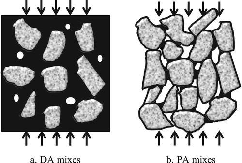
Figure 4. Illustration of the MT model for PA mixes.

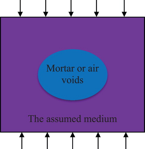
Under the assumption presented above, Equation (10) can be rewritten as Equation (11), where the subscripts ‘mix’, ‘mor’, ‘void’ and ‘ske’ denote PA mixes, mortar, air voids and the stone-on-stone skeleton, respectively. The terms ‘$f_{\mathrm{ske}}{\mathbf{C}}_{\mathrm{ske}}^{\ast }:{\mathbf{A}}_{\mathrm{ske}}^{\ast }$’ and ‘$f_{\mathrm{mor}}{\mathbf{C}}_{\mathrm{mor}}^{\ast }:{\mathbf{A}}_{\mathrm{mor}}^{\ast }$’ represent the contributions of the stone-on-stone skeleton and the mortar to the stiffness of PA mixes, respectively.

By considering all the phases to be isotropic and the inclusions to be spherical, the value of ${\mathbf{C}}_{\mathrm{mix}}^{\ast }$ can be calculated by Equations (12 and 13) in terms of the bulk modulus κ* and the shear modulus μ*, respectively. It is highlighted here that in reality neither the materials are isotropic nor the inclusions are spherical. However, many research studies (Lackner et al. 2005, Yin et al. 2008, Kim 2009, Underwood and Kim 2013) have demonstrated that both assumptions can be made to obtain solutions within reasonable accuracy. Furthermore, since the aim of this paper is to provide a methodology to estimate the stiffness of the stone-on-stone skeleton of PA mixes, the impacts of the non-spherical shapes of inclusions and anisotropic material properties of the mix are beyond the scope of this paper and will be considered in the future research.(11) $\begin{array}{rl}{\mathbf{C}}_{\mathrm{mix}}^{\ast }=& f_{\mathrm{ske}}{\mathbf{C}}_{\mathrm{ske}}^{\ast }:{\mathbf{A}}_{\mathrm{ske}}^{\ast }+f_{\mathrm{mor}}{\mathbf{C}}_{\mathrm{mor}}^{\ast }:{\mathbf{A}}_{\mathrm{mor}}^{\ast }\\ =& (f_{\mathrm{ske}}{\mathbf{C}}_{\mathrm{ske}}^{\ast }+f_{\mathrm{mor}}{\mathbf{C}}_{\mathrm{mor}}^{\ast }:{\mathbf{T}}_{\mathrm{mor}}^{\ast }):\\ & (f_{\mathrm{ske}}\mathbf{I}+f_{\mathrm{mor}}{\mathbf{T}}_{\mathrm{mor}}^{\ast }+f_{\mathrm{void}}{\mathbf{T}}_{\mathrm{void}}^{\ast }{)}^{-1}\end{array}$(11) (12) $\begin{array}{rl}3{\kappa }_{\mathrm{mix}}^{\ast }& =\{f_{\mathrm{ske}}\cdot 3{\kappa }_{\mathrm{ske}}^{\ast }+f_{\mathrm{mor}}\cdot 3{\kappa }_{\mathrm{mor}}^{\ast }\cdot {[1+{\alpha }_{\mathrm{ske}}^{\ast }\cdot 3\kappa {{}_{\mathrm{ske}}^{\ast }}^{-1}\cdot (3{\kappa }_{\mathrm{mor}}^{\ast }-3{\kappa }_{\mathrm{ske}}^{\ast })]}^{-1}\}\\ & \cdot {\left\{\begin{array}{c}{f}_{\mathrm{ske}}+f_{\mathrm{mor}}\cdot [1+{\alpha }_{\mathrm{ske}}^{\ast }\cdot 3\kappa {{}_{\mathrm{ske}}^{\ast }}^{-1}\cdot (3{\kappa }_{\mathrm{mor}}^{\ast }-3{\kappa }_{\mathrm{ske}}^{\ast }){]}^{-1}\\ +f_{\mathrm{void}}\cdot [1+{\alpha }_{\mathrm{ske}}^{\ast }\cdot 3\kappa {{}_{\mathrm{ske}}^{\ast }}^{-1}\cdot (-3{\kappa }_{\mathrm{ske}}^{\ast }){]}^{-1}\end{array}\right\}}^{-1}\end{array}$(12) (13) $\begin{array}{rl}{\mu }_{\mathrm{mix}}^{\ast }=& \{f_{\mathrm{ske}}\cdot 2{\mu }_{\mathrm{ske}}^{\ast }+f_{\mathrm{mor}}\cdot 2{\mu }_{\mathrm{mor}}^{\ast }\\ & \cdot {[1+{\beta }_{\mathrm{ske}}^{\ast }\cdot 2\mu {{}_{\mathrm{ske}}^{\ast }}^{-1}\cdot (2{\mu }_{\mathrm{mor}}^{\ast }-2{\mu }_{\mathrm{ske}}^{\ast })]}^{-1}\}\\ & \cdot {\left\{\begin{array}{c}{f}_{\mathrm{ske}}+f_{\mathrm{mor}}\cdot [1+{\beta }_{\mathrm{ske}}^{\ast }\cdot 2\mu {{}_{\mathrm{ske}}^{\ast }}^{-1}\cdot (2{\mu }_{\mathrm{mor}}^{\ast }-2{\mu }_{\mathrm{ske}}^{\ast }){]}^{-1}\\ +f_{\mathrm{void}}\cdot [1+{\beta }_{\mathrm{ske}}^{\ast }\cdot 2\mu {{}_{\mathrm{ske}}^{\ast }}^{-1}\cdot (-2{\mu }_{\mathrm{ske}}^{\ast }){]}^{-1}\end{array}\right\}}^{-1}\end{array}$(13)

with(14) ${\alpha }_{\mathrm{ske}}^{\ast }={\displaystyle \frac{3{\kappa }_{\mathrm{ske}}^{\ast }}{3{\kappa }_{\mathrm{ske}}^{\ast }+4{\mu }_{\mathrm{ske}}^{\ast }},{\beta }_{\mathrm{ske}}^{\ast }={\displaystyle \frac{6({\kappa }_{\mathrm{ske}}^{\ast }+2{\mu }_{\mathrm{ske}}^{\ast })}{5(3{\kappa }_{\mathrm{ske}}^{\ast }+4{\mu }_{\mathrm{ske}}^{\ast })}}}$(14) In Equations (12 and 13), it is difficult to get an explicit expression in terms of ${\kappa }_{\mathrm{ske}}^{\ast }$ and ${\mu }_{\mathrm{ske}}^{\ast }$, therefore numerical methods are necessary. One of the most commonly used numerical methods for solving a nonlinear equation (f (x) = 0) is the Newton-Raphson method (Galántai 2000). This method uses the following formula to approximate the solution of f (x) in an iterative procedure:(15) $x_{i+1}=x_i-{\displaystyle \frac{f(x_i)}{f^{\mathrm{\prime }}(x_i)}}$(15) where x_n and x_n + 1 are the estimates of x in step n and n + 1, respectively, and f (x) is the derivative of f (x). In the residual form, Equations (12 and 13) can be rewritten as (16) and (17) respectively. The values of ${\kappa }_{\mathrm{ske}}^{\ast }$ and ${\mu }_{\mathrm{ske}}^{\ast }$ at each step can be calculated by solving Equation (18). The iteration stops when the error term |e|, as shown in Equation (19), is within the expected tolerance (0.0001 in this study).(16) $\begin{array}{rl}{R}_{\kappa }=& 3{\kappa }_{\mathrm{mix}}^{\ast }-\{f_{\mathrm{ske}}\cdot 3{\kappa }_{\mathrm{ske}}^{\ast }+f_{\mathrm{mor}}\cdot 3{\kappa }_{\mathrm{mor}}^{\ast }\\ & \cdot {[1+{\alpha }_{\mathrm{ske}}^{\ast }\cdot 3\kappa {{}_{\mathrm{ske}}^{\ast }}^{-1}\cdot (3{\kappa }_{\mathrm{mor}}^{\ast }-3{\kappa }_{\mathrm{ske}}^{\ast })]}^{-1}\}\\ & \cdot {\left\{\begin{array}{c}{f}_{\mathrm{ske}}+f_{\mathrm{mor}}\cdot [1+{\alpha }_{\mathrm{ske}}^{\ast }\cdot 3\kappa {{}_{\mathrm{ske}}^{\ast }}^{-1}\cdot (3{\kappa }_{\mathrm{mor}}^{\ast }-3{\kappa }_{\mathrm{ske}}^{\ast }){]}^{-1}\\ +f_{\mathrm{void}}\cdot [1+{\alpha }_{\mathrm{ske}}^{\ast }\cdot 3\kappa {{}_{\mathrm{ske}}^{\ast }}^{-1}\cdot (-3{\kappa }_{\mathrm{ske}}^{\ast }){]}^{-1}\end{array}\right\}}^{-1}\end{array}$(16) (17) $\begin{array}{rl}{R}_{\mu }=& 2{\mu }_{\mathrm{mix}}^{\ast }-\{f_{\mathrm{ske}}\cdot 2{\mu }_{\mathrm{ske}}^{\ast }+f_{\mathrm{mor}}\cdot 2{\mu }_{\mathrm{mor}}^{\ast }\\ & \cdot {[1+{\beta }_{\mathrm{ske}}^{\ast }\cdot 2\mu {{}_{\mathrm{ske}}^{\ast }}^{-1}\cdot (2{\mu }_{\mathrm{mor}}^{\ast }-2{\mu }_{\mathrm{ske}}^{\ast })]}^{-1}\}\\ & \cdot {\left\{\begin{array}{c}{f}_{\mathrm{ske}}+f_{\mathrm{mor}}\cdot [1+{\beta }_{\mathrm{ske}}^{\ast }\cdot 2\mu {{}_{\mathrm{ske}}^{\ast }}^{-1}\cdot (2{\mu }_{\mathrm{mor}}^{\ast }-2{\mu }_{\mathrm{ske}}^{\ast }){]}^{-1}\\ +f_{\mathrm{void}}\cdot [1+{\beta }_{\mathrm{ske}}^{\ast }\cdot 2\mu {{}_{\mathrm{ske}}^{\ast }}^{-1}\cdot (-2{\mu }_{\mathrm{ske}}^{\ast }){]}^{-1}\end{array}\right\}}^{-1}\end{array}$(17) (18) ${\left[\begin{array}{c}{\kappa }_{\mathrm{ske}}^{\ast }\\ {\mu }_{\mathrm{ske}}^{\ast }\end{array}\right]}_{i+1}={\left[\begin{array}{c}{\kappa }_{\mathrm{ske}}^{\ast }\\ {\mu }_{\mathrm{ske}}^{\ast }\end{array}\right]}_i-[\begin{array}{c}{\displaystyle \frac{\mathrm{\partial }{R}_{\kappa }}{\mathrm{\partial }{\kappa }_{\mathrm{ske}}^{\ast }}}\\ {\displaystyle \frac{\mathrm{\partial }{R}_{\mu }}{\mathrm{\partial }{\kappa }_{\mathrm{ske}}^{\ast }}}\end{array}{\begin{array}{c}{\displaystyle \frac{\mathrm{\partial }{R}_{\kappa }}{\mathrm{\partial }{\mu }_{\mathrm{ske}}^{\ast }}}\\ {\displaystyle \frac{\mathrm{\partial }{R}_{\mu }}{\mathrm{\partial }{\mu }_{\mathrm{ske}}^{\ast }}}\end{array}]}_i^{-1}{\left[\begin{array}{c}{R}_{\kappa }\\ R_{\mu }\end{array}\right]}_i$(18) (19) $|e|=\Vert {\left[\begin{array}{c}{\kappa }_{\mathrm{ske}}^{\ast }\\ {\mu }_{\mathrm{ske}}^{\ast }\end{array}\right]}_{i+1}-{\left[\begin{array}{c}{\kappa }_{\mathrm{ske}}^{\ast }\\ {\mu }_{\mathrm{ske}}^{\ast }\end{array}\right]}_i\Vert$(19)

Materials and experiments

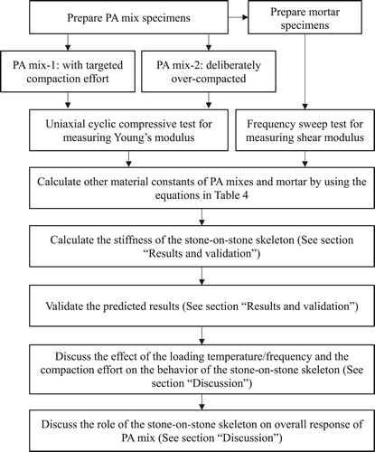
As shown in the flowchart of Figure 5, the study was carried out in different steps which are briefly described in this paragraph. PA mix specimens were prepared according to the standards (NEN-EN 2007, CROW 2015) while mortar specimens were prepared according to previous research works (Huurman 2007, Dijkhuis 2016). Half of the total PA mix specimens were compacted at targeted air voids and the rest were deliberately over-compacted. The Young’s modulus of PA mix specimens ($E_{\mathrm{mix}}^{\ast }$) was measured by using the uniaxial cyclic compressive test, whereas ${\mu }_{\mathrm{mor}}^{\ast }$ was measured from the frequency sweep test, as described later in the paper. Other material constants (${\kappa }_{\mathrm{mix}}^{\ast }$, ${\mu }_{\mathrm{mix}}^{\ast }$ and ${\kappa }_{\mathrm{mor}}^{\ast }$) were calculated by using equations shown in Table 4. The stiffness of the stone-on-stone skeleton was further calculated by using Equations (16 and 17). Two methods of validations were carried out. In the first validation method, the predicted stiffness was compared against the prediction from Christensen’s model; whereas in the second method, the modulus of the mix was back-calculated using Equations (12 and 13). The obtained results were used to discuss the effect of the loading temperature/frequency & the compaction effort on the behaviour of the stone-on-stone skeleton, and the role of the skeleton on overall mix response was highlighted.

Figure 5. Workflow diagram.

Specimens preparation

Specimens preparation for PA mixes

The preparation of PA mixes specimens conforms to the Dutch standard specifications (NEN-EN 2007, CROW 2015). The content of asphalt binder (Pen 70–100) is 4.3% by the total weight of the mix and the gradation of the aggregates is shown in Table 1. These specimens, with a diameter of 100 mm and a height of 150 mm, were compacted via a gyratory compactor. The reference compaction effort was applied to half of the specimens (labelled as PA mix-1) to target the designed air voids content of 18%. In order to create a different stone-on-stone skeleton and investigate the effect of the compaction effort on the stiffness of the skeleton, more compaction effort was deliberately applied on the remaining specimens (labelled as PA mix-2).

Table 1. Gradation and density of aggregates.

Size (mm)	16	11.2	8	5.6	2	0.5	0.18	0.125	0.063	Filler
% Passing	98	77	44	22	15	14	9	6	4	0
Density (kg/m^3)	2686	2686	2678	2670	2673	2658	2658	2658	2658	2638

The volume fraction of each phase, f_ske, f_mor and f_void, is shown in Table 2. The value of f_void was measured from laboratory tests according to ASTM D7063 (ASTM 2011). The values of f_ske and f_mor were obtained on the basis of the measured densities of aggregates (Table 1) and the assumed density of 1030 kg/m³ for asphalt binder.

Table 2 . The volume fraction of each phase.

PA mixes	Stone-on-stone skeleton	Mortar	Air voids
PA mix-1	0.624	0.197	0.179
PA mix-2	0.66	0.208	0.132

Specimens preparation for mortar

In this study, mortar specimens contained sand particles smaller than 0.5 mm, filler and asphalt binder. The proportioning of the fine aggregates in mortar was kept the same as that in the full mixture, but it was normalised with respect to the largest sieve in the mortar (0.5 mm), see Table 3. The content of the asphalt binder was calculated as 23% by the total weight of the mortar specimen.

Table 3. Gradation of aggregates in mortar.

Size (mm)	0.5	0.18	0.125	0.063	Filler
Gradation (% Passing)	100	62	39	29	0

A brief overview of the preparation of mortar specimens is presented as follows. At first, the preheated asphalt binder, filler and sand particles were mixed by hand to obtain the mortar material. In order to make mortar flow smoothly, the material and the special designed mould (see Figure 6(a)) were heated up in the oven at 160°C for 30 min. The mortar was slowly poured into the mould to prevent the formation of air voids. Then, the filled mould was placed back in the oven at 160°C for 10 min to remove air bubbles in the mortar. After cooling down the mould for 10 min at room temperature and around 24 h in the freezer, the specimens were removed from the mould.

Figure 6. Preparation of mortar specimens.

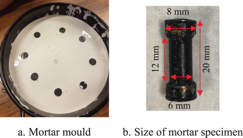
The size of the obtained specimens is 6 mm in diameter and 12 mm in height, see Figure 6(b). In order to clamp specimens on the Dynamic Shear Rheology (DSR) device, steel rings of 1 mm in thickness and 4 mm in height are attached at the top and bottom (Huurman 2007). It is highlighted here that the air voids content of the mortar specimens in this study was assumed to be very low and thus no compaction effort was applied during the fabrication. This assumption was verified by performing Nano CT scans which showed that the air voids content of mortar was lower than 0.9%.

Laboratory tests

DSR test

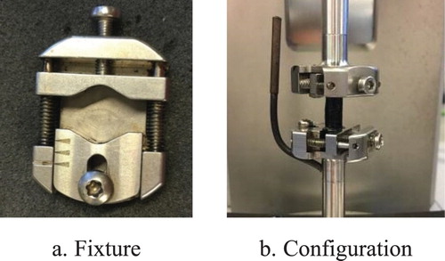
The value of ${\mu }_{\mathrm{mor}}^{\ast }$ was measured by using the so-called ‘Column Configuration’ of the DSR device, as shown in Figure 7. This measurement was on the basis of three replicates. Frequency sweep tests were performed in a frequency range of 50 to 0.1 Hz, at four different temperatures, −10°C, 4°C, 21°C and 37°C; and at each temperature, constant small strains were applied.

Figure 7. DSR setup for mortar tests.

Uniaxial cyclic compressive test

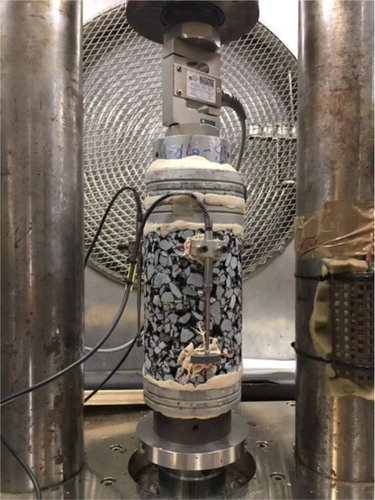
The value of $E_{\mathrm{mix}}^{\ast }$ was measured by using the Universal Testing Machine (UTM), see Figure 8. Uniaxial cyclic compressive forces were applied on the specimens at four temperatures of −10°C, 4°C, 21°C and 37°C. At each temperature, six frequencies of 20, 10, 5, 1, 0.5 and 0.1 Hz were performed. The displacements were measured by using three linear variable differential transformers (LVDT) which were equally distributed around the specimens. In this test, three replicates were used for each PA mix.

Figure 8. Setup for the uniaxial cyclic compressive test.

Calculation of material constants of PA mixes and mortar

On the basis of the measured results of $E_{\mathrm{mix}}^{\ast }$ and ${\mu }_{\mathrm{mor}}^{\ast }$, the values of ${\kappa }_{\mathrm{mix}}^{\ast }$, ${\mu }_{\mathrm{mix}}^{\ast }$ and ${\kappa }_{\mathrm{mor}}^{\ast }$ were calculated by using the equations in Table 4. It is highlighted here that the values of ν_mix and ν_mor are supposed to be frequency and temperature dependent (Di Benedetto et al. 2007, Kim and Buttlar 2011); however, it is difficult to accurately measure these values due to the limitations of testing devices. Furthermore, sensitivity analysis conducted by the authors indicated that the predicted stiffness of the stone-on-stone skeleton is not very sensitive to the values of ν_mix and ν_mor. An increase of ν_mix and ν_mor from 0.1 to 0.45 reduces the predicted results by less than 5%. Therefore, constant values of ν_mix and ν_mor were assumed in this study, as followed by other researchers (Kim and Little 2004, Abbas et al. 2005).

Table 4. Mechanical properties of PA mixes and mortar.

Material constants	Mix	Mortar
Shear modulus	${\mu }_{\mathrm{mix}}^{\ast }={\displaystyle \frac{E_{\mathrm{mix}}^{\ast }}{2(1+{\nu }_{\mathrm{mix}})}}$	${\mu }_{\mathrm{mor}}^{\ast }$
Bulk modulus	${\kappa }_{\mathrm{mix}}^{\ast }={\displaystyle \frac{E_{\mathrm{mix}}^{\ast }}{3(1-2{\nu }_{\mathrm{mix}})}}$	${\kappa }_{\mathrm{mor}}^{\ast }={\displaystyle \frac{2{\mu }_{\mathrm{mor}}^{\ast }(1+{\nu }_{\mathrm{mor}})}{3(1-2{\nu }_{\mathrm{mor}})}}$
Poisson’s ratio	νmix = 0.3	νmor = 0.3
Young’s modulus	$E_{\mathrm{mix}}^{\ast }$	$E_{\mathrm{mor}}^{\ast }=2{\mu }_{\mathrm{mor}}^{\ast }(1+{\nu }_{\mathrm{mor}})$

Results and validation

Predicted stiffness of the stone-on-stone skeleton

By substituting the volume fraction (Table 2) and the mechanical properties of each phase (Table 4) into Equations (16 and 17), the values of ${\mu }_{\mathrm{ske}}^{\ast }$ and ${\kappa }_{\mathrm{ske}}^{\ast }$ were obtained. The complex Young’s modulus of the stone-on-stone skeleton $E_{\mathrm{ske}}^{\ast }$ was further calculated by using Equation (20). 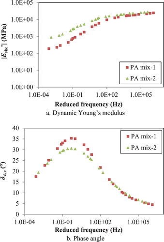The obtained average values of $|E_{\mathrm{ske}}^{\ast }|$ and δ_ske of three replicates are presented in Figure 9. The coefficient of variation was calculated as less than 6% at high frequencies; while it increased up to 15% at low frequencies. This can be explained by the fact that at low frequencies (high temperatures), the applied force was low and thus easier to be affected by the electronic noise of the measurement system (Underwood 2011).(20) $E_{\mathrm{ske}}^{\ast }={\displaystyle \frac{9{\kappa }_{\mathrm{ske}}^{\ast }{\mu }_{\mathrm{ske}}^{\ast }}{3{\kappa }_{\mathrm{ske}}^{\ast }+{\mu }_{\mathrm{ske}}^{\ast }}}$(20)

Figure 9. Predicted results of the stone-on-stone skeleton’s stiffness.

Validation of the proposed methodology for predicting the stiffness of the stone-on-stone skeleton

Validation by Christensen’s model

Christensen’s model (Christensen et al. 2003) is one of the most commonly used semi-empirical models for predicting the stiffness of asphalt mixture. In the previous work of the authors (Zhang et al. 2018b), a modified arrangement of Christensen’s model was proposed for predicting the stiffness of a PA mix. In the modified arrangement, the total volumes of binder (considered as mortar in this paper), aggregates and air voids are considered to be in parallel, see Figure 10. Accordingly, the general equation proposed by Christensen was also modified, as shown in Equation (21), where a new term P_a (aggregate organisation factor) was introduced. The in-detail description of P_a is beyond the scope of this study and can be found elsewhere (Zhang et al. 2018b).(21) $|E_{\mathrm{mix}}^{\ast }|=f_{\mathrm{agg}}{P}_{\mathrm{a}}{E}_{\mathrm{agg}}+f_{\mathrm{mor}}|E_{\mathrm{mor}}^{\ast }|$(21) where f_agg and E_agg are the volume fraction and the Young’s modulus of aggregates, respectively.

Figure 10. Modified arrangement of the Christensen’s model.

The term ‘f_agg P_a E_agg’ in Equation (21) represents the temperature/frequency dependent contribution of aggregates’ stiffness in the total mix. A comparison of Equation (21) with the MT model (see Equation (11)) shows that the term ‘f_agg P_a E_agg’ is similar to ‘$f_{\mathrm{ske}}{\mathbf{C}}_{ske}^{\ast }:{\mathbf{A}}_{ske}^{\ast }$’ (or $E_{\mathrm{mix}\mathrm{\_}\mathrm{agg}}^{\ast }$ in this case). Since both terms account for the contribution of aggregates to the stiffness of PA mixes, the values of f_agg P_a E_agg and $E_{\mathrm{mix}\mathrm{\_}\mathrm{agg}}^{\ast }$ can be compared to indirectly validate the proposed methodology.

By rearranging Equation (21), the value of f_agg P_a E_agg can be obtained, see Equation (22); and the value of $E_{\mathrm{mix}\mathrm{\_}\mathrm{agg}}^{\ast }$ can be obtained by rearranging Equations (12 and 13), see Equations (23–25). Figure 11 shows the comparison between f_agg P_a E_agg and $|E_{\mathrm{mix}\mathrm{\_}\mathrm{agg}}^{\ast }|$. It can be seen that for both mixes, i.e. PA mix-1 and PA mix-2, the values of $|E_{\mathrm{mix}\mathrm{\_}\mathrm{agg}}^{\ast }|$ and f_agg P_a E_agg match quite well along the equality line.(22) $f_{\mathrm{agg}}{P}_{\mathrm{a}}{E}_{\mathrm{agg}}=|E_{\mathrm{mix}}^{\ast }|-f_{\mathrm{mor}}|E_{\mathrm{mor}}^{\ast }|$(22) (23) $\begin{array}{rl}& 3{\kappa }_{\mathrm{mix}\mathrm{\_}\mathrm{agg}}^{\ast }=f_{\mathrm{ske}}\cdot 3{\kappa }_{\mathrm{ske}}^{\ast }\\ & \cdot {\left\{\begin{array}{c}{f}_{\mathrm{ske}}+f_{\mathrm{mor}}\cdot [1+{\alpha }_{\mathrm{ske}}^{\ast }\cdot 3\kappa {{}_{\mathrm{ske}}^{\ast }}^{-1}\cdot (3{\kappa }_{\mathrm{mor}}^{\ast }-3{\kappa }_{\mathrm{ske}}^{\ast }){]}^{-1}\\ +f_{\mathrm{void}}\cdot [1+{\alpha }_{\mathrm{ske}}^{\ast }\cdot 3\kappa {{}_{\mathrm{ske}}^{\ast }}^{-1}\cdot (-3{\kappa }_{\mathrm{ske}}^{\ast }){]}^{-1}\end{array}\right\}}^{-1}\end{array}$(23)

(24) $\begin{array}{rl}& 2{\mu }_{\mathrm{mix}\mathrm{\_}\mathrm{agg}}^{\ast }=f_{\mathrm{ske}}\cdot 2{\mu }_{\mathrm{ske}}^{\ast }\\ & \cdot {\left\{\begin{array}{c}{f}_{\mathrm{ske}}+f_{\mathrm{mor}}\cdot [1+{\beta }_{\mathrm{ske}}^{\ast }\cdot 2\mu {{}_{\mathrm{ske}}^{\ast }}^{-1}\cdot (2{\mu }_{\mathrm{mor}}^{\ast }-2{\mu }_{\mathrm{ske}}^{\ast }){]}^{-1}\\ +f_{\mathrm{void}}\cdot [1+{\beta }_{\mathrm{ske}}^{\ast }\cdot 2\mu {{}_{\mathrm{ske}}^{\ast }}^{-1}\cdot (-2{\mu }_{\mathrm{ske}}^{\ast }){]}^{-1}\end{array}\right\}}^{-1}\end{array}$(24) (25) $E_{\mathrm{mix}\mathrm{\_}\mathrm{agg}}^{\ast }={\displaystyle \frac{9{\kappa }_{\mathrm{mix}\mathrm{\_}\mathrm{agg}}^{\ast }{\mu }_{\mathrm{mix}\mathrm{\_}\mathrm{agg}}^{\ast }}{3{\kappa }_{\mathrm{mix}\mathrm{\_}\mathrm{agg}}^{\ast }+{\mu }_{\mathrm{mix}\mathrm{\_}\mathrm{agg}}^{\ast }}}$(25)

Figure 11. Comparison between $|E_{\mathrm{mix}\mathrm{\_}\mathrm{agg}}^{\ast }|$ and f_aggP_aE_agg.

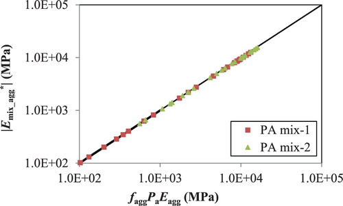
The above comparison clearly demonstrates the applicability of the proposed methodology. However, the comparison could not validate the applicability of the methodology in the prediction of the phase angle (δ_ske), because Christensen’s model cannot predict δ_mix from the properties of different phases for a given mix. Therefore, the back-calculated values of $E_{\mathrm{mix}}^{\ast }$ were compared with the experimental values of $E_{\mathrm{mix}}^{\ast }$.

Validation by back-calculation method

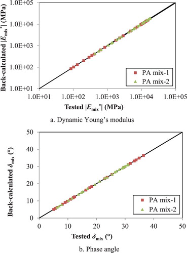
By substituting predicted results of ${\kappa }_{\mathrm{ske}}^{\ast }$ and ${\mu }_{\mathrm{ske}}^{\ast }$ into Equations (12 and 13), $|E_{\mathrm{mix}}^{\ast }|$ and δ_mix were obtained, see Figure 12. The back-calculated values and the experimental results show a good agreement. This shows that the proposed method is suitable not only for elastic properties but also for predicting viscoelastic material properties.

Figure 12. Comparison between tested $E_{\mathrm{mix}}^{\ast }$ and back-calculated $E_{\mathrm{mix}}^{\ast }$.

Discussion

Effect of temperature/frequency on the behaviour of the stone-on-stone skeleton

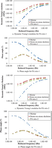
From Figure 9, it can be seen that the predicted values of $|E_{\mathrm{ske}}^{\ast }|$ and δ_ske are both frequency dependent. A brief explanation of the observation will be provided below.

Influence of frequency/temperature on $|E_{\mathrm{ske}}^{\ast }|$

The value of $|E_{\mathrm{ske}}^{\ast }|$ decreases with the decrease of frequency. For example, on a log-log scale a decrease of frequency from 10⁵ to 10⁻³ Hz reduces the value of $|E_{\mathrm{ske}}^{\ast }|$ by approximately 48% for PA mix-1 and 34% for PA mix-2. At first glance, it may seem to be counter-intuitive that the value of $E_{\mathrm{ske}}^{\ast }$ depends on frequency. It is noted here that $E_{\mathrm{ske}}^{\ast }$ reflects the stiffness of the mortar coated stone-on-stone skeleton rather than the uncoated stone-on-stone skeleton. It is easier to understand the behaviour of the coated stone-on-stone skeleton by examining extreme conditions, i.e. low temperature (or high frequency) and high temperature (or low frequency), see Figure 13.

Figure 13. The behaviour of the stone-on-stone skeleton at different frequencies/temperatures.

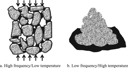
At low temperatures since the binder is stiff enough to form a stable network, the stone particles are expected to be bonded together. In this case, the applied load can be distributed to different particles via the skeleton network. Thus, the whole stone-on-stone skeleton acts together to provide stiffness.

On the contrary, at high temperatures, see Figure 13(b), the soft binder might not be able to bind particles well and thus the stone-on-stone skeleton would form a weaker network. In this case, once a load is applied on the mix, the load will mostly be transferred via the direct contacts between the stone particles. Since the total stone-binder contact area is expected to dominate over the stone-stone contact area, the overall stiffness of the stone-on-stone skeleton decreases drastically.

Influence of frequency/temperature on δ_ske

The value of δ_ske initially increases and further starts to decrease beyond a peak point. A decrease of frequency from 10⁵ to 0.5 Hz increases δ_ske from 5 degrees to peak values of 35 and 30 degrees for PA mix-1 and PA mix-2, respectively. Whereas, a further decrease from 0.5 to 10⁻³ Hz reduces the value of δ_ske to 20 degrees. This could be explained by the fact that at low temperatures the phase angle of the stone-on-stone skeleton heavily relies on the viscous properties of the binder, which increase with temperature. Whereas, at high temperatures, the phase angle would be governed by the particle-particle contact response. Since the response of the direct contact between two particles is elastic, the overall behaviour of the stone-on-stone skeleton also tends to be elastic (lower values of δ_ske). This could also explain the peak formation in the middle range of temperatures.

It is noted here that the mechanism shown in Figure 13 is a hypothesis that could explain the results obtained from the tests. The validation of this hypothesis is beyond the scope of this paper, which will be conducted in the future research.

Effect of compaction effort on the behaviour of the stone-on-stone skeleton

In order to understand the role of the compaction effort, two mixes with the same properties but different compaction effort were prepared in the laboratory. The predicted results on the basis of the experimental data are compared in Figure 9. It can be clearly observed that the amount of the compaction effort affects the behaviour of the coated stone-on-stone skeleton:

• The values of $|E_{\mathrm{ske}}^{\ast }|$ of PA mix-2, which has a higher compaction effort, are found to be higher than the values of $|E_{\mathrm{ske}}^{\ast }|$ of PA mix-1.

• The lack of proper compaction effort is significantly reflected at lower frequencies. For example, at a frequency of 10⁵ Hz, $|E_{\mathrm{ske}}^{\ast }|$ of PA mix-2 is higher by 12%; while at a frequency of 10⁻³ Hz, it is approximately five times of $|E_{\mathrm{ske}}^{\ast }|$ of PA mix-1.

Influence of compaction effort on $|E_{\mathrm{ske}}^{\ast }|$

With more compaction effort, it is expected that stone particles will be more in contact with each other, resulting in a more pronounced stone-on-stone skeleton, as illustrated in Figure 14. It can be clearly seen that in a more compacted PA mix, there are much more contact areas between different stones. Therefore, the load can be transferred more efficiently providing a better load bearing capacity.

Figure 14. The behaviour of the stone-on-stone skeleton with different amount of compaction effort.

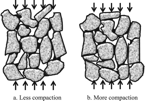
As discussed in the previous section, at high temperatures, the load transfer characteristics are mainly governed by the stone-stone contact. Under the high-temperature condition, the lack of the stone-binder contact in combination with the lack of the stone-stone contact (due to insufficient compaction), result in a further reduction of the stiffness.

Role of the stone-on-stone skeleton on the overall response of PA mixes

In order to examine the role of the stone-on-stone skeleton on the overall response of PA mixes, the predicted $E_{\mathrm{ske}}^{\ast }$ was compared to $E_{\mathrm{mor}}^{\ast }$ and $E_{\mathrm{mix}}^{\ast }$, see Figure 15.

Figure 15. Comparison of stiffness between the stone-on-stone skeleton with mortar and PA mixes.

It can be observed that at higher frequencies, $E_{\mathrm{mix}}^{\ast }$ is close to $E_{\mathrm{mor}}^{\ast }$, whereas at lower frequencies $E_{\mathrm{mix}}^{\ast }$ is much higher than $E_{\mathrm{mor}}^{\ast }$. For example, at a frequency of 10⁵ Hz, $E_{\mathrm{mix}}^{\ast }$ is higher than $E_{\mathrm{mor}}^{\ast }$ by 23% and 42% for PA mix-1 and PA mix-2, respectively; while at a frequency of 10⁻³ Hz, $E_{\mathrm{mix}}^{\ast }$ is more than 500 times higher than $E_{\mathrm{mor}}^{\ast }$. This can be explained by the fact that at high frequencies, asphalt binder is stiff enough to make a significant contribution to the load-bearing capacity of the mortar. At low frequencies, the mortar cannot withstand significant load because not only the binder is too soft but also there is a lack of a skeletal framework. On the contrary, the binder in the mix is also not able to provide any significant resistance but the availability of the stone-on-stone skeleton provides additional resistance. This shows that the stone-on-stone skeleton plays an important role in the overall response of a mix, which is in line with the findings from previous studies (Alvarez et al. 2010, Mansour and Putman 2013, Chen and Wong 2017).

Furthermore, it can also be seen that the shapes of $E_{\mathrm{mix}}^{\ast }$ and $E_{\mathrm{mor}}^{\ast }$ differ from each other; while $E_{\mathrm{mix}}^{\ast }$ has a similar shape as predicted $E_{\mathrm{ske}}^{\ast }$. This indicates that the frequency responses of both the mix and the stone-on-stone skeleton (coated) are similar in nature. It can be hypothesised that the load transfer mechanism of the stone-on-stone skeleton in a way affects the shape of $|E_{\mathrm{mix}}^{\ast }|$.

Conclusions

This paper presents a methodology to estimate the stiffness of the stone-on-stone skeleton and its role in the behaviour of PA mixes. By means of micromechanical models, the stiffness of the stone-on-stone skeleton was predicted on the basis of the properties of mortar and PA mixes. Based on the predictions, the effects of the loading temperatures/frequencies and the compaction effort on the behaviour of the stone-on-stone skeleton, as well as the role of the skeleton on the overall response of PA mixes, were discussed. From the predicted results and the discussion, the following conclusions can be drawn:

• The stiffness of the stone-on-stone skeleton is frequency dependent. The magnitude of the stiffness decreases with the decrease of frequency, and the phase angle initially increases and further starts to decrease beyond a peak point.

• The stiffness of the stone-on-stone skeleton is also dependent on the compaction effort. The lack of proper compaction effort induces lower stiffness of the stone-on-stone skeleton, which is significantly reflected in the lower frequencies range.

• The frequency dependency of the stiffness of the stone-on-stone skeleton can be explained by the load transfer mechanisms at different temperatures. At low temperatures, the transfer of the load relies on the bonding effect of the binder; while at high temperatures, the load is transferred via the direct contact between stone particles.

• More compaction effort results in more direct contact between stone particles, which provides a better load-bearing capacity of the stone-on-stone skeleton especially in the higher temperatures range.

• The stone-on-stone skeleton plays an important role in the overall response of PA mixes. The stiffness of the mix has a similar shape as the predicted stiffness of the stone-on-stone skeleton, which indicates that the frequency responses of both the mix and the stone-on-stone skeleton are similar in nature.

Recommendation for the future research

The limitation of this study is that the stiffness of the stone-on-stone skeleton was obtained on the basis of laboratory tests of PA mixes. In the future research, the current work will be extended to enable the prediction of the stone-on-stone skeleton’s stiffness exclusively on the basis of the properties of mortar and aggregate particles. On the basis of the obtained stiffness of the skeleton, the stiffness of PA mixes will be determined and the propensity of a given PA mix for ravelling will be further analysed.

Disclosure statement

No potential conflict of interest was reported by the authors.

References

- Abbas, A., et al., 2005. Modelling asphalt mastic stiffness using discrete element analysis and micromechanics-based models. International Journal of Pavement Engineering, 6 (2), 137–146.
- Alvarez, A.E., et al., 2010. Stone-on-stone contact of permeable friction course mixtures. Journal of Materials in Civil Engineering, 22 (11), 1129–1138.
- Alvarez, A.E., Mora, J.C., and Espinosa, L.V., 2018. Quantification of stone-on-stone contact in permeable friction course mixtures based on image analysis. Construction and Building Materials, 165, 462–471.
- Anupam, K., et al., 2014. Study of cornering maneuvers of a pneumatic tire on asphalt pavement surfaces using the finite element method. Transportation Research Record: Journal of the Transportation Research Board, 2457 (1), 129–139.
- Anupam, K., et al., 2016. Microstructural analysis of porous asphalt concrete mix subjected to rolling truck tire loads. Transportation Research Record: Journal of the Transportation Research Board, 2575, 113–122.
- Anupam, K., et al., 2017. Finite element framework for the computation of runway friction of aircraft tires. Journal of Transportation Research Record, 2641, 126–138.
- ASTM, 2011. Standard test method for effective porosity and effective air voids of compacted bituminous paving mixture samples.
- Benveniste, Y., 1987. A new approach to the application of mori-tanaka’s theory in composite materials. Mechanics of Materials, 6 (2), 147–157.
- Budiansky, B., 1965. On the elastic moduli of some heterogeneous materials. Journal of the Mechanics and Physics of Solids, 13 (4), 223–227.
- Buttlar, W.G.R., 1996. Evaluation of empirical and theoretical models to determine asphalt mixture stiffnesses at low temperatures. Journal of the Association of Asphalt Paving Technologists, 65, 99–141.
- Buttlar, W., et al., 1999. Understanding asphalt mastic behavior through micromechanics. Transportation Research Record: Journal of the Transportation Research Board, 1681, 157–169.
- Chen, M.J. and Wong, Y.D., 2017. Evaluation of the development of aggregate packing in porous asphalt mixture using discrete element method simulation. Road Materials and Pavement Design, 18 (1), 64–85.
- Christensen, R.M. and Lo, K.H., 1979. Solutions for effective shear properties in three phase sphere and cylinder models. Journal of the Mechanics and Physics of Solids, 27 (4), 315–330.
- Christensen, D.W., Pellinen, T., and Bonaquist, R.F., 2003. Hirsch model for estimating the modulus of asphalt concrete. Journal of the Association of Asphalt Paving Technologists, 72, 97–121.
- CROW, 2015. Standaard RAW bepalingen. Ede, The Netherlands.
- Di Benedetto, H., Delaporte, B., and Sauzéat, C., 2007. Three-dimensional linear behavior of bituminous materials: experiments and modeling. International Journal of Geomechanics, 7 (2), 149–157.
- Dijkhuis, S.L., 2016. Fatigue and healing of asphalt mortar. Delft, The Netherlands: Delft University of Technology.
- Eshelby, J.D., 1957. The determination of the elastic field of an ellipsoidal inclusion, and related problems. Proceedings of the Royal Society of London. Series A. Mathematical and Physical Sciences, 241 (1226), 376–396.
- Galántai, A., 2000. The theory of newton’s method. Journal of Computational and Applied Mathematics, 124 (1), 25–44.
- Ghauch, Z.G., Ozer, H., and Al-Qadi, I.L., 2015. Micromechanical finite element modeling of moisture damage in bituminous composite materials. Construction and Building Materials, 80, 9–17.
- Ghossein, E. and Lévesque, M., 2014. A comprehensive validation of analytical homogenization models: the case of ellipsoidal particles reinforced composites. Mechanics of Materials, 75, 135–150.
- Hardiman, H., 2004. Application of packing theory on grading design for porous asphalt mixtures. Civil Engineering Dimension, 6 (2), 57–63.
- Hashin, Z., 1970. Complex moduli of viscoelastic composites—i. General theory and application to particulate composites. International Journal of Solids and Structures, 6 (5), 539–552.
- Hill, R., 1965. A self-consistent mechanics of composite materials. Journal of the Mechanics and Physics of Solids, 13 (4), 213–222.
- Huurman, M., 2007. Lifetime optimisation tool, lot.
- Kandhal, P.S. and Mallick, R.B., 1988. Open graded asphalt friction course: state of the practice.
- Kim, M., 2009. Development of differential scheme micromechanics modeling framework for predictions of hot-mix asphalt (hma) complex modulus and experimental validations. Urbana, Illinois: University of Illinois at Urbana-Champaign.
- Kim, M. and Buttlar, W.G., 2011. Differential scheme effective medium theory for hot-mix asphalt |e*| prediction. Journal of Materials in Civil Engineering, 23 (1), 69–78.
- Kim, Y.-R. and Little, D.N., 2004. Linear viscoelastic analysis of asphalt mastics. Journal of Materials in Civil Engineering, 16 (2), 122–132.
- Kringos, N. and Scarpas, A., 2005. Raveling of asphaltic mixes due to water damage: computational identification of controlling parameters. Transportation Research Record: Journal of the Transportation Research Board, 1929, 79–87.
- Kringos, N. and Scarpas, A., 2008. Physical and mechanical moisture susceptibility of asphaltic mixtures. International Journal of Solids and Structures, 45 (9), 2671–2685.
- Lackner, R., et al., 2005. Is low-temperature creep of asphalt mastic independent of filler shape and mineralogy? - arguments from multiscale analysis. Journal of Materials in Civil Engineering, 17 (5), 485–491.
- Li, J., et al., 2019. Three-dimensional simulation of aggregate and asphalt mixture using parameterized shape and size gradation. Journal of Materials in Civil Engineering, 31 (3), 1–9.
- Manrique-Sanchez, L., Caro, S., and Arámbula-Mercado, E., 2018. Numerical modelling of ravelling in porous friction courses (pfc). Road Materials and Pavement Design, 19 (3), 668–689.
- Mansour, T.N. and Putman, B.J., 2013. Influence of aggregate gradation on the performance properties of porous asphalt mixtures. Journal of Materials in Civil Engineering, 25 (2), 281–288.
- Mo, L.T., et al., 2007. Investigation into stress states in porous asphalt concrete on the basis of fe-modelling. Finite Elements in Analysis and Design, 43 (4), 333–343.
- Mo, L., et al., 2009. Ravelling investigation of porous asphalt concrete based on fatigue characteristics of bitumen–stone adhesion and mortar. Materials & Design, 30 (1), 170–179.
- Mori, T. and Tanaka, K., 1973. Average stress in matrix and average elastic energy of materials with misfitting inclusions. Acta Metallurgica, 21 (5), 571–574.
- Nen-En, 2007. Specimen preparation by gyratory compactor. Bituminous Mixtures - Test Methods for Hot Mix Asphalt.
- Norris, A.N., 1985. A differential scheme for the effective moduli of composites. Mechanics of Materials, 4 (1), 1–16.
- Shu, X. and Huang, B., 2008. Dynamic modulus prediction of hma mixtures based on the viscoelastic micromechanical model. Journal of Materials in Civil Engineering, 20 (8), 530–538.
- Shu, X. and Huang, B., 2009. Predicting dynamic modulus of asphalt mixtures with differential method. Road Materials and Pavement Design, 10 (2), 337–359.
- Siddharthan, R.V., Krishnamenon, N., and Sebaaly, P.E., 2000. Finite-layer approach to pavement response evaluation. Transportation Research Record: Journal of the Transportation Research Board, 1709 (1), 43–49.
- Siddharthan, R.V., Yao, J., and Sebaaly, P.E., 1998. Pavement strain from moving dynamic 3d load distribution. Journal of Transportation Engineering, 124 (6), 557–566.
- Srirangam, S.K., et al., 2015. Study of influence of operating parameters on braking friction and rolling resistance. Transportation Research Record: Journal of the Transportation Research Board, 2525 (1), 79–90.
- Underwood, B.S., 2011. Multiscale constitutive modeling of asphalt concrete.
- Underwood, B.S. and Kim, Y.R., 2013. Effect of volumetric factors on the mechanical behavior of asphalt fine aggregate matrix and the relationship to asphalt mixture properties. Construction and Building Materials, 49, 672–681.
- Underwood, B.S. and Kim, Y.R., 2014. A four phase micro-mechanical model for asphalt mastic modulus. Mechanics of Materials, 75, 13–33.
- Wang, J., et al., 2016. Behaviour of asphalt concrete mixtures under tri-axial compression. Construction and Building Materials, 105, 269–274.
- Yin, H.M., et al., 2008. Assessment of existing micro-mechanical models for asphalt mastics considering viscoelastic effects. Road Materials and Pavement Design, 9 (1), 31–57.
- Zhang, H., et al., 2018a. Comparison of different micromechanical models for predicting the effective properties of open graded mixes. Transportation Research Record: Journal of the Transportation Research Board, 2672 (28), 404–415.
- Zhang, H., et al., 2018b. Issues in the prediction of the mechanical properties of open graded mixes. Transportation Research Record: Journal of the Transportation Research Board, 2672 (40), 32–40.