Investigating mechanical characteristics of aggregate structure for road materials

ABSTRACT

Aggregate structure plays a significant role in the pavement performance of road materials. However, there is a lack of fundamental understanding of mechanical characteristics and evolution characteristics of the aggregate structure in the existing research. To understand this complex structure, laboratory tests and numerical simulations using the discrete element method were used to investigate macroscopic mechanical properties of aggregate structure and microscopic aggregate contact forces, thus revealing the mechanical role of each size aggregate and evolution characteristics of the aggregate structure. Based on this, the specification gradations of road materials were optimised to build a strong aggregate structure. Laboratory tests and engineering application show that road materials using the proposed gradation can exhibit improved pavement performance and engineering effects.

KEYWORDS:

• Road materials
• aggregate structure
• macroscopic mechanical property
• microscopic aggregate contact force
• discrete element method (DEM)

1. Introduction

As particulate composite materials, road materials are composed of coarse aggregates, fine aggregates and binders (asphalt or cement). Among the constituents, the aggregates occupy the biggest volume proportion within road materials, which interlock with each other and form a stable structure to transmit and distribute traffic loads. Obviously, the aggregate structure plays an important role in the performance of road materials. Shen et al. (2010, 2011) specifically stated in their researches that aggregate structure is the primary factor influencing the performance of road materials, which is confirmed by Dukatz (1989), Dondi et al. (2012), Vignali et al. (2014) and Zhang et al. (2016). Therefore, an in-depth analysis of aggregate structure characteristics has an important signification.

At present, there are two general methods to investigate the aggregate structure characteristics: experimental tests and numerical techniques.

Experimental tests employ the volumetric indices of aggregate structure to evaluate packing characteristics. In the National Center for Asphalt Technology, the aggregate structure is assumed to be established when the voids of the aggregate structure are less than the dry-rodded voids (Brown et al. 1997). Ghabchi et al. (2015) analysed the effect of shape parameters and gradation on the aggregate packing characteristics. However, the mechanical resistance to deformation is the essential feature of aggregate structure rather than the volumetric property (Azéma et al. 2010, 2012, Mostofinejad et al. 2012, Visseq et al. 2012, Chen et al. 2015). Experimental tests are designed to investigate macroscopic mechanical characteristics of aggregate structure and reveal the effect on each size of aggregates of the microscopic mechanical characteristics.

To solve the above problems, numerical techniques are used to study the mechanical mechanisms of aggregate structure. Shashidhar et al. (2000) used photo-elastic methods to analyse the force transmission path of aggregate packing. Shen et al. (2011) analysed contact force distribution between aggregates using an ideal sphere. Bernal et al. (1970) studied the contact structure of aggregate packing using the paint and optical method. Gatchalian et al. (2006) applied the X-ray to evaluate the resistance of the aggregate structure to degradation in asphalt concrete. Masad (2004) investigated the morphology of aggregate structure in asphalt mixes using X-ray. Dondi et al. (2012) investigated the combined effect of grain shape and angularity on the packing and stability of aggregate structure for asphalt concrete using regular spheres based on DEM simulations. Yideti and Birgisson et al. (2013, 2014a, 2014b) analysed the effect of the particle size and its distribution on the aggregate structure characteristics and built the primary and secondary structure system. Chen et al. (2015) performed DEM simulation to study the micromechanical characteristics of aggregate structure for asphalt concrete using an ideal sphere. Xiao et al. (2016) analysed the gradation and packing characteristics of aggregate structure-based aggregate imaging and DEM simulations. These studies contribute to the improvement of our understanding of mechanical characteristics of the aggregate structure. However, there are the following drawbacks in the literature of DEM models for asphalt concrete: (a) the irregular aggregate shape is not considered, (b) the contribution of each sieve size to the aggregate structure is still not fully understood and (c) the evolution characteristics of aggregate structure are not revealed.

In response to the above questions, we investigate the macroscopic and microscopic mechanical characteristics of the aggregate structure, analyse the mechanical role of each size aggregate to the aggregate structure and reveal the evolution characteristics of the aggregate structure through experimental tests and DEM simulations in this study. Based on this, the specification gradations of road materials are optimised to build a stronger aggregate structure, thus providing an improved pavement performance.

2. Laboratory test

2.1. Test preparation

To investigate the mechanical behaviour of aggregate structure, a modified experimental test method based on the triaxial testing system is used in this study, as shown in Figure 1.

Figure 1. Sketch of loading device.

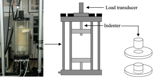
In the test method, a modified loading device like that used in the CBR test is used instead of the original loading device used in the standard triaxial test. The loading device is composed of one cylindrical indenter with a diameter of 5cm and one circular press plate. The cylindrical indenter and the press plate are under control using two independent loading systems. The loading rate is 1 mm/min. Moreover, according to the Chinese specification ‘Test Methods of Soils for Highway Engineering’ (Ministry of Communications of PRC 2007), the requirement of sample size and aggregate diameter is that: (a) the sample diameter is 5 times of the maximum aggregate diameter (when the maximum aggregate diameter is larger than 10 mm) and the sample height is 2–2.5 times of sample diameter in triaxial tests, and (b) the sample size is Φ150×h120 mm and the maximum aggregate diameter must be less than 40 mm in CBR tests. In this study, the proposed test method combines the characteristics of triaxial tests and CBR tests. The sample size is set as Φ150×h300 mm, and the maximum aggregate diameter is 31.5 mm. In the following section, the reasonability of sample size is demonstrated from a view of the stability of testing data via the coefficient of variation. Other testing devices are identical to that used in the standard triaxial test.

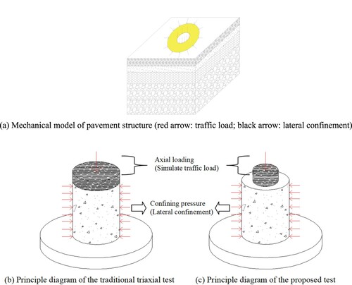
Figure 2 plots the mechanical model of pavement structure and principle diagram of different tests. It can be found that although the vehicle load doesn’t directly act on the materials in the yellow region, it still indirectly affects these materials. The comparison with Figure 2(a,b) shows that the traditional triaxial test cannot clearly reflect the mechanical behaviour of the materials outside the range of the loading zone. Hence, as shown in the Figure 2(b,c), it is reasonable to speculate that the proposed test approach can simulate the actual stress state of pavement materials more closely.

Figure 2. Principle diagram of the proposed test. (a) Mechanical model of pavement structure (red arrow: traffic load; black arrow: lateral confinement). (b) Principle diagram of the traditional triaxial test (c) Principle diagram of the proposed test.

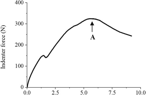
Figure 3 plots a relationship between indenter-force and indenter-displacement. The peak indenter-force (point A) is used to evaluate the macroscopic mechanical property of the aggregate structure.

Figure 3. Relationship between indenter-force and indenter-displacement.

2.2. Test programme

In this study, limestone aggregates of Chuzhou city in Anhui Province of China are used in laboratory tests. 19–31.5 mm aggregates (D1), 13.2–19 mm aggregates (D2), 9.5–13.2 mm aggregates (D3), 4.75–9.5 mm aggregates (D4), 2.36–4.75 mm aggregates (D5), 1.18–2.36 mm aggregates (D6) and 0.6–1.18 mm aggregates (D7) are employed to analyse the mechanical characteristics of the aggregate structure. Five confining pressures are selected: 50, 100, 150, 200, 300 and 400 KPa. For each material, composition and test condition, six specimens are tested successfully.

The testing programme is shown as follows:

1. The specimen formed of D1 is denoted as P1. The peak indenter-force of P1 is investigated at different confining pressures.

2. Peak indenter-forces of aggregate packing using different proportions of P1 and D2 are investigated. When the peak indenter-force reached the maximum value, the proportion of P1 and D2 is recorded and named ‘the optimal proportion’. The specimen formed using the optimal proportion is denoted as P2.

3. Peak indenter-forces of aggregate packing using different proportions of P2 and D3 are investigated. When the peak indenter-force reached the maximum value, the proportion of P2 and D3 is recorded and named ‘the optimal proportion’. The specimen mixed using the optimal proportion is denoted as P3.

4. By analogy, P4 (D1–D4), P5 (D1–D5), P6 (D1–D6) and P7 (D1–D7) are determined.

The detailed test results are listed in Tables 1–7. Under 50 KPa confining pressure, P1, P2, P3, P4, P5, P6 and P7 are tests No.1, No.8, No.40, No.68, No.93, No.108 and No.133, respectively. Under 100 KPa confining pressure, P1, P2, P3, P4, P5, P6 and P7 are tests No.2, No.16, No.46, No.73, No.98, No.113 and No.138, respectively. Under 150KPa confining pressure, P1, P2, P3, P4, P5, P6 and P7 are tests No.3, No.23, No.52, No.78, No.93, No.118 and No.143, respectively. Under 250KPa confining pressure, P1, P2, P3, P4, P5, P6 and P7 are tests No.4, No.30, No.58, No.83, No.98, No.123 and No.148, respectively. Under 350KPa confining pressure, P1, P2, P3, P4, P5, P6 and P7 are tests No.5, No.35, No.63, No.88, No.103, No.128 and No.153, respectively. CV is the coefficient of variation and calculated through Equation (1). (1) $CV=\sigma /\mu \times 100\text{\%}$(1) where σ is the standard deviation, and μ is the average value.

Table 1. Lab test results of aggregate packing composed of D1.

No.	Confining pressure (KPa)	Mass fraction (%) of aggregates	Indenter peak-force (N)	CV (%)
1	50	100	119.2	6.9
2	100	100	124.7	6.7
3	150	100	136.7	8.6
4	250	100	144.0	6.2
5	350	100	159.3	3.9

Table 2. Lab test results of aggregate packing composed of D1 and D2.

No.	Confining pressure (kPa)	Mass fraction (%) of aggregates		Indenter peak-force (N)	CV (%)
		D1 (P1)	D2
6	50	90	10	228.1	7.2
7		85	15	238.1	9.7
8		80	20	254.6	9.8
9		75	25	224.8	8.3
10		70	30	181.9	6.5
11		65	35	171.9	6.9
12		60	40	155.4	3.0
13	100	90	10	222.1	6.9
14		85	15	237.7	6.8
15		80	20	248.5	5.3
16		75	25	266.3	4.8
17		70	30	234.7	4.9
18		65	35	189.5	7.6
19		60	40	178.8	9.1
20	150	90	10	216.6	7.8
21		85	15	237.7	7.6
22		80	20	251.0	6.8
23		75	25	277.2	3.9
24		70	30	265.5	6.0
25		65	35	233.0	6.3
26		60	40	205.3	5.5
27	250	85	15	259.6	8.4
28		80	20	283.1	4.0
29		75	25	304.0	9.7
30		70	30	312.3	7.9
31		65	35	269.7	8.1
32		60	40	214.1	4.7
33	350	80	20	303.8	8.5
34		75	25	328.6	7.9
35		70	30	341.7	9.0
36		65	35	308.7	8.8
37		60	40	235.3	6.2

Table 3. Lab test results of aggregate packing composed of D1–D3.

No.	Confining pressure (kPa)	Mass fraction (%) of aggregates			Indenter peak-force (N)	CV (%)
		P2		D3
		D1	D2
38	50	76	19	5	314.6	6.2
39		72	18	10	325.6	8.4
40		68	17	15	334.3	8.3
41		64	16	20	319.9	8.8
42		60	15	25	304.9	9.1
43		56	14	30	287.1	7.7
44	100	71.2	23.8	5	328.3	9.2
45		67.5	22.5	10	339.8	6.1
46		63.7	21.3	15	349.6	7.6
47		60	20	20	333.9	7.8
48		56.2	18.8	25	318.1	7.5
49		52.5	17.5	30	301.2	2.6
50	150	71.3	23.7	5	337.2	8.1
51		67.5	22.5	10	353.3	7.7
52		63.8	21.2	15	374.0	7.2
53		60	20	20	365.5	8.3
54		56.3	18.7	25	358.7	4.4
55		52.5	17.5	30	335.9	8.7
56	250	63	27	10	377.7	5.1
57		59.5	25.5	15	394.6	6.3
58		56	24	20	405.6	9.8
59		52.5	22.5	25	397.1	6.8
60		49	21	30	374.6	7.1
61	350	63	27	10	435.5	8.5
62		59.5	25.5	15	446.6	6.1
63		56	24	20	450.3	8.3
64		52.5	22.5	25	437.1	9.5
65		49	21	30	409.7	9.3

Table 4. Lab test results of aggregate packing composed of D1–D4.

No.	Confining pressure (kPa)	Mass fraction (%) of aggregates				Indenter peak-force (N)	CV (%)
		P3			D4
		D1	D2	D3
66	50	64.6	16.2	14.2	5	386.2	4.6
67		61.2	15.3	13.5	10	398.5	6.6
68		57.8	14.5	12.7	15	408.7	5.5
69		54.4	13.6	12	20	393.2	7.6
70		51	12.7	11.3	25	375.2	8.8
71	100	60.5	20.2	14.3	5	404.2	5.8
72		57.4	19.1	13.5	10	417.9	6.1
73		54.2	18	12.8	15	427.7	6.9
74		51	17	12	20	410.6	7.1
75		47.8	15.9	11.3	25	391.3	8.3
76	150	60.6	20.1	14.3	5	428.6	9.9
77		57.4	19.1	13.5	10	439.2	7.1
78		54.2	18	12.8	15	446.4	7.2
79		51	17	12	20	437.1	6.8
80		47.9	15.9	11.2	25	429.2	6.6
81	250	53.2	22.8	19	5	490.1	6.1
82		50.4	21.6	18	10	496.2	6.9
83		47.6	20.4	17	15	499.6	8.9
84		44.8	19.2	16	20	488.8	5.3
85		42	18	15	25	468.6	6.4
86	350	53.2	22.8	19	5	548.6	9.1
87		50.4	21.6	18	10	558.5	7.3
88		47.6	20.4	17	15	561.3	6.2
89		44.8	19.2	16	20	549.3	3.8
90		42	18	15	25	530.1	6.1

Table 5. Lab test results of aggregate packing composed of D1–D5.

No.	Confining pressure (kPa)	Mass fraction (%) of aggregates					Indenter peak-force (N)	CV (%)
		P4				D5
		D1	D2	D3	D4
91	50	54.9	13.8	12	14.3	5	428.4	8.0
92		52	13.1	11.4	13.5	10	443.1	5.5
93		49.1	12.3	10.8	12.8	15	450.1	6.6
94		46.2	11.6	10.2	12	20	435.5	5.8
95		43.3	10.9	9.5	11.3	25	415.3	6.2
96	100	51.5	17.1	12.1	14.3	5	447.1	9.2
97		48.8	16.2	11.5	13.5	10	462.6	9.1
98		46	15.3	10.9	12.8	15	470.7	4.6
99		43.4	14.4	10.2	12	20	454.6	8.1
100		40.6	13.5	9.6	11.3	25	433.1	6.2
101	150	51.5	17.1	12.2	14.2	5	481.9	8.3
102		48.8	16.2	11.5	13.5	10	491.1	10.0
93		45.6	15.4	11.1	12.9	15	500.8	9.1
94		43.4	14.4	10.2	12	20	486.9	5.5
95		40.7	13.5	9.6	11.2	25	471.1	8.9
96	250	45.2	19.4	16.2	14.2	5	540.5	6.1
97		42.8	18.4	15.3	13.5	10	551.5	9.0
98		40.5	17.3	14.5	12.7	15	555.1	5.8
99		38.1	16.3	13.6	12	20	547.0	6.7
100		35.7	15.3	12.8	11.2	25	531.5	9.5
101	350	45.2	19.4	16.2	14.2	5	608.6	9.1
102		42.8	18.4	15.3	13.5	10	619.9	3.7
103		40.5	17.3	14.5	12.7	15	621.3	5.0
104		38.1	16.3	13.6	12	20	606.6	7.6
105		35.7	15.3	12.8	11.2	25	594.0	6.2

Table 6. Lab test results of aggregate packing composed of D–D6.

No.	Confining pressure (kPa)	Mass fraction (%) of aggregates						Indenter peak-force (N)	CV (%)
		P5					D6
		D1	D2	D3	D4	D5
106	50	46.6	11.7	10.2	12.2	14.3	5	444.3	8.4
107		44.2	11.1	9.7	11.5	13.5	10	458.7	4.3
108		41.7	10.5	9.2	10.8	12.8	15	465.5	9.6
109		39.3	9.9	8.6	10.2	12	20	451.6	6.9
110		36.8	9.2	8.1	9.6	11.3	25	431.7	6.3
111	100	43.7	14.5	10.3	12.2	14.3	5	464.0	7.3
112		41.4	13.8	9.8	11.5	13.5	10	479.0	4.5
113		39.1	13	9.3	10.8	12.8	15	486.8	9.5
114		36.8	12.3	8.7	10.2	12	20	471.1	8.8
115		34.5	11.5	8.1	9.6	11.3	25	450.9	8.7
116	150	43.8	14.5	10.4	12.1	14.2	5	498.5	8.4
117		41.5	13.8	9.8	11.4	13.5	10	509.3	9.6
118		39.2	13	9.3	10.8	12.7	15	515.1	7.0
119		36.9	12.2	8.7	10.2	12	20	498.5	8.9
120		34.6	11.5	8.2	9.5	11.2	25	479.7	4.3
121	250	38.4	16.5	13.7	12.1	14.3	5	562.6	7.2
122		36.4	15.6	13	11.5	13.5	10	566.8	8.6
123		34.4	14.7	12.3	10.8	12.8	15	571.9	8.6
124		32.4	13.9	11.6	10.2	12	20	561.2	5.9
125		30.3	13	10.8	9.6	11.3	25	539.3	9.1
126	350	38.4	16.5	13.7	12.1	14.3	5	644.3	7.3
127		36.4	15.6	13	11.5	13.5	10	647.8	6.3
128		34.4	14.7	12.3	10.8	12.8	15	655.1	6.2
129		32.4	13.9	11.6	10.2	12	20	647.0	7.2
130		30.3	13	10.8	9.6	11.3	25	634.4	8.6

Table 7. Lab test results of aggregate packing composed of D1–D7.

No.	Confining pressure (kPa)	Mass fraction (%) of aggregates							Indenter peak-force (N)	CV (%)
		P6						D7
		D1	D2	D3	D4	D5	D6
131	50	39.6	10	8.7	10.3	12.2	14.3	5	445.8	8.3
132		37.5	9.5	8.3	9.7	11.5	13.5	10	460.1	7.6
133		35.4	8.9	7.8	9.2	10.9	12.8	15	467.0	7.7
134		33.4	8.4	7.4	8.6	10.2	12	20	453.0	8.0
135		31.2	7.9	6.9	8.1	9.6	11.3	25	433.3	6.0
136	100	37.1	12.3	8.8	10.3	12.2	14.3	5	465.7	9.1
137		35.2	11.7	8.4	9.7	11.5	13.5	10	480.4	7.7
138		33.2	11	7.9	9.2	10.9	12.8	15	488.4	6.2
139		31.3	10.4	7.5	8.6	10.2	12	20	473.1	6.7
140		29.3	9.7	7	8.1	9.6	11.3	25	453.7	6.6
141	150	37.2	12.4	8.8	10.3	12.1	14.2	5	496.8	7.6
142		35.3	11.7	8.4	9.7	11.4	13.5	10	507.6	5.1
143		33.3	11.1	7.9	9.2	10.8	12.7	15	518.8	3.3
144		31.4	10.4	7.4	8.6	10.16	12	20	506.6	9.8
145		29.4	9.8	7.0	8.1	9.5	11.2	25	491.9	8.7
146	250	32.7	14	11.7	10.3	12.1	14.2	5	568.2	5.5
147		31	13.2	11.1	9.7	11.5	13.5	10	576.7	9.6
148		29.2	12.5	10.5	9.2	10.9	12.7	15	579.3	8.8
149		27.5	11.8	9.8	8.6	10.3	12	20	568.7	6.2
150		25.8	11	9.2	8.1	9.6	11.3	25	559.1	9.0
151	350	32.7	14	11.7	10.3	12.1	14.2	5	651.0	7.1
152		31	13.2	11.1	9.7	11.5	13.5	10	656.9	5.3
153		29.2	12.5	10.5	9.2	10.9	12.7	15	658.4	9.5
154		27.5	11.8	9.8	8.6	10.3	12	20	651.1	4.4
155		25.8	11	9.2	8.1	9.6	11.3	25	641.9	6.6

As shown in Tables 1–7, the coefficients of variation are all less than 10%, which meets the specification requirement of the triaxial test (20%) and the CBR test (12%), showing that the relationship of sample size and aggregate diameter used in this study can ensure the testing stability. The peak indenter-forces of P1–P7 are used to evaluate the macroscopic mechanical performance of aggregate structure in Section 2.3. The optimal aggregate proportions in P1–P7 are used to optimise the aggregate gradation in Section 4.

2.3. Indenter peak-force

The peak indenter force (f) of P1–P7 are shown in Figure 4.

Figure 4. f of P1–P7.

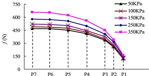
In Figure 4, the peak indenter force rapidly grows with the addition of D1–D3. The peak indenter force of P3 is, on average, 2.82 times higher than that of P1. Subsequently, the growth of peak indenter force becomes slow with the addition of D4–D5. The peak indenter force of P5 is, on average, 1.36 times higher than that of P3. Particularly, the peak indenter force almost stops growing with the addition of D6 and D7. The peak indenter force of P7 is only, on average, 1.04 times higher than that of P5. It shows that D1–D3 is the main section of aggregate structure and D6–D7 have little impact on the formation of the aggregate structure. In the following section, we will elucidate these phenomena from a view of microscopic aggregate contact force.

3. DEM simulation

To analyse the mechanical behaviour of the aggregate structure further, a series of 2D-DEM simulations containing irregular aggregate elements are used to investigate the microscopic contact forces of aggregates in this section.

3.1. Numerical model preparation

In a general discussion on 2D analysis, Brooks (2009) described 2D ‘flatland’ as a space with ‘just enough room for interesting and useful things to arise’. This is certainly the case in DEM analyses in granular materials. O’Sullivan (2011) considered that ‘The overall response of a 2D system is qualitatively similar to a 3D system, i.e. phenomena such as the dependence of the material response on the stress state, hysteresis, dilation upon shearing, etc. are all observed’. As a 2D DEM model captures many of the key complex mechanical response features unique to granular materials, it can be used with a large degree of confidence to study the internal mechanics of granular materials and to assess how different particle-scale parameters influence the overall material response.

Based on the 2D-DEM software package PFC^2D (Itasca Consulting Group 2004), Figure 5 shows the modelling procedure for building numerical samples containing irregular aggregate elements.

Figure 5. Procedure for a randomly generated numerical model.

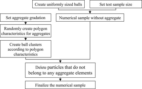
The detailed modelling process is as follow:

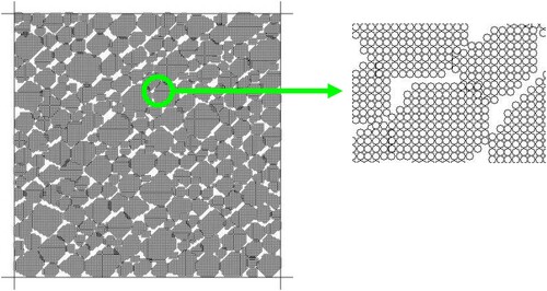
According to the sample size, the densely assembled particles with the same diameter are generated in a regular pattern to build the DEM model without aggregates. Polygon characteristics (central coordinates, vertex coordinates and the number of vertexes) are created randomly. The length of the longest diagonal and the area of the polygon should be calculated and recorded. For one group of polygon characteristics, a polygon zone can be obtained by connecting all the vertexes in sequence. The particles within the polygon zone are grouped to simulate one aggregate element. Similarly, all the aggregate elements are created according to the corresponding polygon characteristics. Particles that do not belong to any aggregate elements are deleted. Figure 6 plots the completed DEM model.

Figure 6. Numerical specimen.

It should be noted that:

1. The length of the longest polygon diagonal is used to determine the aggregate specification (D1, D2, … , D7);

2. The total area of polygons corresponding to different aggregates can be controlled through Equation (2) (derivation process is shown in Appendix), so that these polygons match the aggregate proportion in different aggregate packing (P1, P2, … , P7);

3. These polygons cannot overlap with each other. (2) $S_{Di}={\displaystyle \frac{dh{P}_{Di}}{{\rho }_{Di}}{\rho }_{max}}$(2) where S_Di is the total area of polygons corresponding to aggregate Di, d is the specimen diameter, h is the specimen height, P_Di is the proportion of aggregate Di, ρ_Di is the density of aggregate Di, and ρ_max is the maximum dry density.

The above can be controlled through the FISH programming language of PFC software.

3.2. Numerical test process

The numerical test (Figure 7) is developed to investigate the mechanical characteristics of the aggregate structure. The detailed process of the numerical test is as follows.

Figure 7. Numerical specimen.

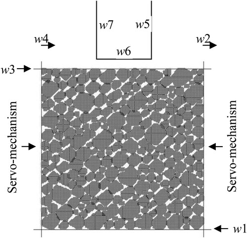
Step 1: Aggregate packing using irregular polygons according to section 3.1 can be generated in a square region composed of four rigid walls (w1–w4).

Step 2: A numerical ‘servo-mechanism’ introduced by ‘Itasca Consulting Group’ is used to control velocities of w2 and w4 to make the confining stress acting on the walls equal to the target value. The ‘servo-mechanism’ algorithm functions during the whole numerical test and can be expressed as follows: (3) $v^{t+1}-v^t=\mathrm{\Delta }\sigma \alpha A/k_{n}N$(3) where v^{t +1} and v^t are the velocity of the target wall at time t + 1 and t, Δσ is the difference between required confining stress and measured confining stress acting on the target wall, α is the relaxation factor, A is the target wall’s area, and k_n and N are the average normal stiffness and the total number of contacts between the target wall and particles, respectively.

Step 3: Three rigid walls (w5–w7) are generated to simulate the indenter which penetrates into the numerical aggregate packing using the constant speed. During the penetration process, the indenter force and displacement should be recorded.

3.3. Verification

The linear contact model embedded in PFC is used in numerical simulations, which contain the reasonable constitutive relation and is recommended to characterise the mechanical behaviour of unbound particle packing by PFC (Itasca Consulting Group 2004). Due to the detailed physical modelling and the special calculative mechanism, PFC can simulate complex particle packing using relatively simple parameters. Moreover, the same contact model and parameter system (normal stiffness k_n, shear stiffness k_s and friction coefficient μ) based on PFC has successfully simulated the mechanical behaviour of the aggregate structure in the existing studies (Zeghal 2004, Uthus et al. 2008, Chen et al. 2015) and delivered satisfactory simulation results. The contact normal stiffness k_n and the contact shear stiffness k_s are calculated through Equation (4). (4) $k_n=2Et{k}_s=2Gt$(4) where E is the Young’s modulus, G is the shear modulus, and t is the initial disk thickness. In PFC software, the initial disk thickness is equal to the standard unit length (1m). After calculating and inputting model parameters, the disk thickness should be redefined according to the ball diameter using the PFC command ‘set disk t’.

Moreover, a limitation in the approach taken herein is that the micro-structure is idealised as a 2D structure, while in reality, the 3D effect will influence the strength of the aggregate structure. In this study, although the irregular shape of 2D particle has been simulated using the randomising algorithm, the 2D model is impossible to represent the 3D particle shape directly. In response, as a common trick in the DEM-simulations, adopting a high value of friction coefficient (compared to the actual value of aggregates) to the 2D particle is widely accepted to simulate the effect of 3D shape indirectly (Wang et al. 2014, Li et al. 2019, Tang et al. 2019), so as to offset the error derived from the difference between 2D and 3D shape as much as possible. Figure 8 plots the variations of the average values of the errors (P1–P7) between simulation results and laboratory data in the case of using different friction coefficients and the same k_n and k_s.

Figure 8. Average values of the errors (P1–P7) in the case of using different friction coefficients.

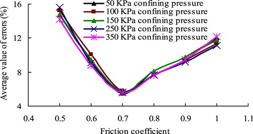
As shown in Figure 8, it can be found that the average values of the errors (P1–P7) at different confining pressures are in general running at a comparatively low level when the friction coefficient is equal to 0.7. Hence, the friction coefficient is set to 0.7 in this study.

Finally, the input parameters are listed in Table 8.

Table 8. Input parameters for DEM simulations.

Contact normal stiffness	Contact Shear stiffness	Friction coefficient
460 MPa	177 MPa	0.7

The comparison between simulation results and laboratory data is shown in Table 9.

Table 9. Errors between laboratory data and simulation results.

Confining pressure/KPa	Aggregate packing	Error (%) of the peak indenter force	Confining pressure/KPa	Aggregate packing	Error (%) of the peak indenter force
50	P1	4.87	100	P1	5.22
	P2	6.11		P2	5.07
	P3	6.68		P3	6.07
	P4	4.43		P4	4.44
	P5	5.11		P5	7.58
	P6	5.57		P6	4.55
	P7	5.93		P7	6.77
150	P1	5.61	250	P1	3.89
	P2	4.53		P2	6.62
	P3	6.34		P3	5.96
	P4	7.43		P4	4.87
	P5	5.57		P5	5.83
	P6	5.55		P6	6.78
	P7	5.33		P7	5.22
350	P1	4.82
	P2	6.15
	P3	5.22
	P4	7.77
	P5	5.27
	P6	6.59
	P7	4.37

According to the Chinese specification ‘Test Methods of Soils for Highway Engineering’ (Ministry of Communications of PRC 2007), the error of the repetitive test in the triaxial test and the CBR test must be less than 20% and 12%, respectively. We consider that the numerical test can be treated as another type of repetitive test. As shown in Table 9, the errors of the numerical tests in different conditions are all less than 10%. Hence, it can be speculated that the simulation results have an acceptable match with the laboratory data, indicating the reliability of the proposed numerical test.

Moreover, because of a high computational cost and complexity in conducting 3D micro-models, many current studies of particle packing has focused on performing 2D simulations and achieved satisfactory results (Azéma et al. 2010, 2012, Estrada et al. 2011, Mostofinejad et al. 2012, Visseq et al. 2012, Zhu et al. 2013, Wang et al. 2014, Chen et al. 2017, Li et al. 2019, Tang et al. 2019). Hence, the current DEM approach can provide a useful tool to investigate the mechanical behaviour of the aggregate structure for this study.

In addition, it is worth noticing that the 2D numerical test method proposed in this study contains three parts: the physical model of aggregates packing with irregular sharp, the simulated loading process and the determination of parameters. We consider that the first two parts can be suitable for various conditions. However, the third part (the determination of parameters) is satisfactory only for this study, because the friction coefficient is obtained by fitting the laboratory test results. The reliability of the parameters should be re-verified to ensure the simulation precision when other assumptions outside of this study (e.g. the change of aggregate texture and lithology) are made.

3.4. Simulation results and discussion

In this study, the number and distribution of aggregate contact force in different aggregate packing are investigated when the aggregate structure reaches the ultimate bearing capacity. Aggregate contact forces are divided into three grades (Sun et al. 2010): weak→(0,<{F}), slightly-strong→[{F}, double {F}] and strong→(double {F}, +∞). {F} is the average value of aggregate contact forces.

Table 10 shows the distribution of aggregate contact forces of P1–P7. Thereby, P(f) is the distribution probability of aggregate contact forces and can be calculated as Equation (5). (5) $P(f)=N_i/N_t\times 100\text{\%}$(5) where N_i (i = 1,2,3) is the number of aggregate contact forces in Grade i, and N_t is the total number of aggregate contact forces.

Table 10. Distribution of aggregate contact force in different aggregate packing.

Packing	Confining pressure (KPa)	Index	Grade 1: (double {F}, +∞)	Grade 2: [{F}, double {F}]	Grade 3: (0,<{F})
P1	50	P(f) /%	34.1	30.6	35.3
		Ni	29	26	30
	100	P(f) /%	39.1	36.8	24.1
		Ni	34	32	21
	150	P(f) /%	44.8	41.4	13.8
		Ni	39	36	12
	250	P(f) /%	48.4	43.0	8.6
		Ni	45	40	8
	350	P(f) /%	50	43.8	6.2
		Ni	48	42	6
P2	50	P(f) /%	41.3	24.9	33.8
		Ni	83	50	68
	100	P(f) /%	42.4	30.5	27.1
		Ni	86	62	55
	150	P(f) /%	45.0	35.0	20.0
		Ni	90	70	40
	250	P(f) /%	47.6	38.3	14.1
		Ni	98	79	29
	350	P(f) /%	49.5	40.4	10.1
		Ni	103	84	21
P3	50	P(f) /%	32.6	26.2	41.2
		Ni	126	101	159
	100	P(f) /%	35.2	31.6	33.2
		Ni	136	122	128
	150	P(f) /%	36.8	36.9	26.3
		Ni	143	143	102
	250	P(f) /%	38.6	40.7	20.7
		Ni	151	159	81
	350	P(f) /%	39.7	43.5	16.8
		Ni	157	172	66
P4	50	P(f) /%	27.7	32.1	40.2
		Ni	164	190	238
	100	P(f) /%	29.1	36.7	34.2
		Ni	172	217	202
	150	P(f) /%	30.5	40.6	28.9
		Ni	180	240	171
	250	P(f) /%	31.8	44.8	23.4
		Ni	189	266	139
	350	P(f) /%	33.4	48.1	18.5
		Ni	201	289	111
P5	50	P(f) /%	18.0	32.7	49.3
		Ni	172	312	470
	100	P(f) /%	18.9	39.4	41.7
		Ni	180	376	398
	150	P(f) /%	19.5	45.9	34.6
		Ni	186	439	331
	250	P(f) /%	20.4	53.5	26.1
		Ni	196	513	250
	350	P(f) /%	21.4	59.3	19.3
		Ni	206	571	186
P6	50	P(f) /%	13.1	25.4	61.5
		Ni	172	335	811
	100	P(f) /%	13.9	30.1	56.0
		Ni	183	397	738
	150	P(f) /%	14.3	35.4	50.3
		Ni	188	466	661
	250	P(f) /%	15.2	41.1	43.7
		Ni	201	545	579
	350	P(f) /%	15.9	45.0	39.1
		Ni	211	598	519
P7	50	P(f) /%	9.9	19.1	71.0
		Ni	176	338	1260
	100	P(f) /%	10.5	22.7	66.8
		Ni	186	402	1182
	150	P(f) /%	10.8	26.6	62.6
		Ni	191	471	1109
	250	P(f) /%	11.4	31.0	57.6
		Ni	203	550	1021
	350	P(f) /%	12.2	34.0	53.8
		Ni	217	608	961

Moreover, to analyse the contribution provided by each size aggregates for the aggregate strength, Figure 9 plot the contact force proportion carried by different size aggregates under confining pressure of 100 KPa and 350KPa.

Figure 9. Contact force proportion carried by different size aggregates.

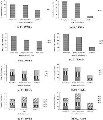
As shown in Table 10 and Figure 9, we can find that the following observations.

In P1–P3, the strong contact forces and slightly-strong contact forces continue to grow, especially the strong contact forces. In P4–P5, the slightly-strong contact forces increase rapidly, while the growth of strong contact forces becomes slow. In P6–P7, the strong contact forces and slightly-strong contact forces almost stop growing. The manner in which strong and slightly-strong contact forces change in different aggregate packings is very consistent with the manner in which peak indenter forces change. The aggregate structure can be defined as a contact force transmission system composed of a series of strong and slightly-strong contact forces.

In P4–P5, although the slightly-strong contact forces increase rapidly, the growth of peak indenter forces becomes slow. It indicates that the role of strong contact forces in the formation of the aggregate strength is higher than that of slightly-strong contact forces.

In P6–P7, there is a large rise in weak contact forces, but the growth of peak indenter forces is not obvious. It shows that weak contact forces have less contribution to enhancing the aggregate structure.

For the same aggregate packing, the total number of contact forces has a little difference under different confining pressures. The weak contact forces reduce with the increase of confining pressure, while the strong and slightly-strong contact forces increase. Meanwhile, the growth rate of slightly-strong contact forces is obviously higher than that of strong contact forces with the increase of confining pressure, implying that the increase of confining pressure mainly transforms weak contact forces into slightly-strong contact forces. The above explains why the peak indenter forces enhance with the increase of confining pressure.

As shown in Figure 9(a)–(n), the strong contact forces are always mainly provided by D1–D3 in different aggregate packing, which shows that D1–D3 is the main section of the aggregate structure. Moreover, D6 and D7 hardly provide any strong contact force or slightly-strong contact force.

As shown in Figure 9(g)–(n), the proportion of slightly-strong contact forces provided by D4 and D5 almost exceeds 50%. Moreover, D4 and D5 also provide about 20% of the strong contact forces in different aggregate packings, and the proportion of slightly-strong contact forces provided by D1–D3 reduces with the addition of D4 and D5. It can be speculated that D4 and D5 transforms the slightly-strong contact forces provided by D1–D3 into strong contact forces, which play a role in structural strengthening for the main aggregate structure. The same thesis would explain why the proportion of strong contact forces provided by D4 and D5 marginally increases with the increase of confining pressure, while that of the slightly-strong contact forces reduces accordingly.

As shown in Figure 9(k)–(n), D6 and D7 provide a large number of weak contact forces for aggregate packing. The proportion of weak contact forces provide by D6 and D7 slightly increases with the increase of confining pressure, because some weak contact forces provided by larger aggregates have been transformed into slightly-strong contact forces under the action of confining pressure. As previously mentioned, weak contact forces have no effect on enhancing the peak indenter-force, which shows that D6 and D7 have little contribution to the formation of aggregate structure strength. In addition, D1–D3 only provide a few weak contact forces.

4. Gradation majorisation

As previously mentioned, D1–D5 (2.36–31.5 mm aggregates) have a significant effect on the aggregate structure strength. Hence, the specification gradations of D1–D5 in different road materials (asphalt concrete and cement stabilised macadam) are optimised to build a stronger aggregate structure in this section. The specification gradations are employed from the Chinese design specifications including ‘Specifications for design of highway asphalt pavement’ (Ministry of Communications of PRC 2017) and ‘Technical specifications for construction of highway road bases’ (Ministry of Communications of PRC 2015) are shown in Table 11.

Table 11. Specification gradation.

Materials	Pass percent/% through the following sieve pore
	31.5 mm	19 mm	13.2 mm	9.5 mm	4.75 mm	2.36m m	1.18 mm	0.6 mm	0.3 mm	0.15 mm	0.075 mm
Asphalt concrete	100	53–72	39–60	31–51	20–40	15–32	10–25	8–18	5–14	3–10	2–6
Cement stabilised macadam	100	68–86	38–58		22–32	16–28	8–15		0–7

4.1. Aggregate structure internal

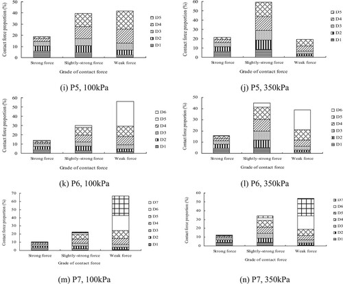
To analyse the aggregate internal structure of D1–D5, the optimal mass fraction of different aggregates in P5 showed in Table 5 is displayed in Figure 10.

Figure 10. The optimal mass proportion of different aggregates in P5.

As shown in Figure 10, the optimal mass fraction of D1, D2, D3, D4 and D5 are 40.5–49.1%, 12.3–17.3%, 10.8–14.5%, 12.7–12.9% and 15%, respectively. The optimal mass proportion of D1 reduces with the increasing confining pressure and that of D2 and D3 increase accordingly, while the total mass proportion of D1 + D2 + D3 has less difference under the three confining pressure. This is due to that the contact forces between aggregates are improved with the increase of confining pressure. Thus some slightly-strong contact forces provided by D2 and D3 are promoted to strong contact forces, so the need for D1 in terms of strong contact forces is reduced. The optimal mass proportion of D4 and D5 hardly changes under different confining pressures.

4.2. Gradation calculation

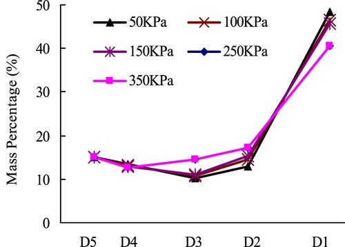
As previously mentioned, D1–D5 (2.36–31.5 mm aggregates) have a significant effect on the aggregate structure strength. Hence, the specification gradation larger than 2.36 mm diameter is recalculated, as shown in Table 12. LP is the total percentage of aggregates whose diameters are larger than 2.36 mm in specification gradation. The proposed gradations are shown in Table 13. Figure 11 displays the comparison between specification gradation and proposed gradation in linear-log scales.

Figure 11. Comparison between specification gradation and proposed gradation. (a) Asphalt concrete. (b) Cement stabilised macadam.

Table 12. Gradation calculation.

Materials	Confining pressure	LP/%	D1:D2:D3:D4:D5	Pass percent/% through the following sieve pore
				31.5 mm	19 mm	13.2 mm	9.5 mm	4.75 mm	2.36 mm
Asphalt concrete	50 KPa	68–85	49.1:12.3:10.8:12.8:15	100	58–66	47–58	38–50	27–41	15–32
	100 KPa		46.0:15.3:10.9:12.8:15	100	60–67	47–58	38–50	27–41	15–32
	150 KPa		45.6:15.4:11.1:12.9:15	100	61–68	48–59	39–51	27–41	15–32
	250 KPa		40.5:17.3:14.5:12.7:15	100	65–72	50–60	39–51	27–41	15–32
	350 KPa		40.5:17.3:14.5:12.7:15	100	65–72	50–60	39–51	27–41	15–32
Cement stabilised macadam	50 KPa	72–84	49.1:12.3:10.8:12.8:15	100	58–64	39–47		26–37	16–28
	100 KPa		46.0:15.3:10.9:12.8:15	100	61–66	39–47		26–37	16–28
	150 KPa		45.6:15.4:11.1:12.9:15	100	62–67	39–48		26–37	16–28

Table 13. Proposed gradation.

Materials	Pass percent/% through the following sieve pore
	31.5 mm	19 mm	13.2 mm	9.5 mm	4.75 mm	2.36 mm	1.18 mm	0.6 mm	0.3 mm	0.15 mm	0.075 mm
Asphalt concrete	100	58–72	47–60	38–51	27–41	15–32	10–25	8–18	5–14	3–10	2–6
Cement stabilised macadam	100	58–66	39–48		26–37	16–28	8–15		0–7

In addition, according to the analysis in Sections 2 and 3, the aggregates whose diameters are smaller than 2.36 mm have little contribution to the formation of aggregate structure strength. Hence, we consider that the interaction between the aggregates (diameter ≤ 2.36 mm) and binders (asphalt or cement) should be more important than the influence of the aggregates (diameter ≤ 2.36 mm) on the aggregate structure in material design. On the other hand, the core aim of this section is to build a strong aggregate structure through the gradation majorisation, and the interaction between the aggregates (diameter ≤ 2.36 mm) and binders is not studied in this paper. Hence, the proportion of the aggregates (diameter ≤ 2.36 mm) follows that in Chinese specifications and does not adopt the optimum proportion in Section 2.

4.3. Pavement performance

To compare the pavement performance of road materials using the proposed gradation and the specification gradation, rutting tests and −10°C bending tests of asphalt concrete and seven-day compressive strength tests and splitting strength tests of cement stabilised macadam are implemented according to Chinese test specifications including ‘Test methods of materials stabilized with inorganic binders for highway engineering’ (Ministry of Communications of PRC 2009) and ‘Standard test methods of bitumen and bituminous mixtures for highway engineering’ (Ministry of Communications of PRC 2011), respectively. The mid-value of the proposed gradation is selected to prepare the samples and test the pavement performance. Proportions of other sizes can be obtained from the Chinese specifications (Ministry of Communications of PRC 2015, 2017). The test results are listed in Table 14. The two Chinese test specifications stipulate that the number of testing replicates for the rutting test, −10°C bending test, compressive strength test and splitting strength test is no less than 3, 6, 9 and 9, respectively. Moreover, the coefficient of variation calculated by Equation (5) is stipulated to be not greater than 20%. In Table 14, AVG is the average value, CV is the coefficient of variation, and NR is the number of testing replicates.

Table 14. Pavement performance of road materials.

Materials	Performance index		Proposed gradation	Specification gradation
Asphalt concrete	Dynamic stability/times·mm^−1	AVG	3589	3151
		CV	6.02%	9.39%
		NR	6	6
	Bending stiffness modulus/MPa	AVG	10,167	10,821
		CV	6.98%	8.93%
		NR	9	9
Cement stabilised macadam	Seven-day compressive strength/MPa	AVG	5.3	4.5
		CV	7.88%	8.67%
		NR	9	9
	Seven-day splitting strength/MPa	AVG	0.78	0.70
		CV	8.03%	9.43%
		NR	9	9

It is observed that road materials using the revised gradation bring improved performance. The seven-day compressive strength and seven-day splitting strength of cement stabilised macadam increase 18% and 11%, respectively. The dynamic stability of asphalt concrete increases by 14%, and the bending stiffness modulus reduces 6% accordingly.

The proposed gradation has been used in the cement stabilised macadam base course of the highway from chuzhou city to chahe city in China, where it achieved a better engineering effect. Figure 12 displays the base course cores using the specification gradation and the proposed gradation.

Figure 12. Base course cores. (a) Specification gradation. (b) Revised gradation.

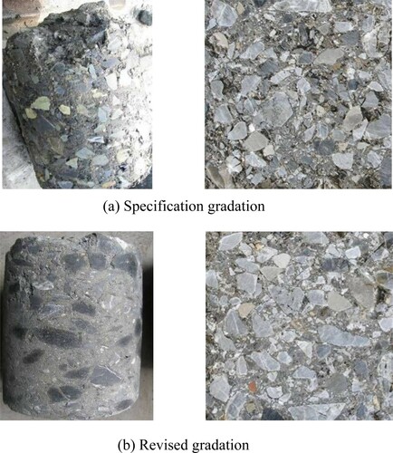
It can be observed that the cores using the designed gradation have a better aggregate interlocked degree than that using the specification gradation. The compressive strength of cores using the proposed gradation is on average 12% higher than that using the specification gradation. It shows that the designed gradation brings a stronger aggregate structure.

5. Conclusions

In this study, the mechanical characteristics of the aggregate structure in road materials are investigated using experimental tests and DEM simulations. The following observations can be made:

• Strong and slightly-strong contact forces play an important role in the load resistant capacity of aggregate structure, especially the strong contact forces, while weak contact forces have less contribution.

• Diameter 9.5–31.5 mm aggregates mainly provide strong contact forces and provide the main structure of aggregate skeleton. The proportion of these aggregates needs to be assured adequately during material design.

• Diameter 2.36– 9.5 mm aggregates bring a large number of slightly-strong contact forces, which play a role in structural strengthening for the main aggregate structure and transform the slightly-strong contact forces provided by diameter 9.5–31.5 mm aggregates to strong contact forces.

• Diameter 0.6–2.36 mm aggregates mainly provide weak contact forces, which have less effect on the formation of aggregate structure. The interaction between these aggregates and binders (asphalt or cement) should be more important than the influence of these aggregates on the aggregate structure in material design.

• The peak indenter-forces increase with increasing confining pressure because the confining pressure transforms the weak and slightly-strong contact forces to slightly-strong and strong contact forces, especially the weak contact forces.

The specification gradation of road materials is optimised to build a stronger aggregate structure. Experimental results and engineering application show that the proposed gradation delivers an improved pavement performance.

In our future research, the evolution mechanisms of contact force network in road materials will be deeply analysed at 3D-scale.

Disclosure statement

No potential conflict of interest was reported by the author(s).

Additional information

Funding

This work was supported by National Natural Science Foundation of China [grant numbers 51808326, 51808327].

Appendix

The DEM simulation software ‘PFC^2D’ is used in this study. In PFC^2D, one of the most important fundamental assumptions is that the density of 3D-entity is equal to that of the corresponding 2D-element. 2D-DEM analysis is not a plane analysis actually, the 2D-element is treated as a element with unit thickness. Hence, the sample density ρ_max can be expressed as, (6) ${\rho }_{max}={\displaystyle \frac{M}{V}={\displaystyle \frac{m}{v}={\displaystyle \frac{m}{St}={\displaystyle \frac{m}{dht}}}}}$(6) where M is the mass of 3D sample, m is the mass of 2D numerical sample, V is the volume of 3D sample, v is the volume of 2D numerical sample, S is the area of the 2D numerical sample, d is the sample diameter, h is the sample height, and t is the thickness of 2D numerical sample.

Thus, S_Di could be calculated through Equations (7)–(9). (7) $m_{Di}=m{P}_{Di}=dht{\rho }_{max}{P}_{Di}$(7) (8) $S_{Di}t={\displaystyle \frac{m_{Di}}{{\rho }_{Di}}={\displaystyle \frac{dht{P}_{Di}}{{\rho }_{Di}}{\rho }_{max}}}$(8) (9) $S_{Di}={\displaystyle \frac{dh{P}_{Di}}{{\rho }_{Di}}{\rho }_{max}}$(9) where S_Di is the total area of polygons corresponding to aggregate Di, m_Di is the mass of aggregate Di in 2D numerical model, P_Di is the proportion of aggregate Di, and ρ_Di is the density of aggregate Di.

References

- Azéma, E., and Radjaï, F, 2010. Stress-strain behavior and geometrical properties of packings of elongated particles. Physical Review E, 81 (5), 703–708. doi: https://doi.org/10.1103/PhysRevE.81.051304
- Azéma, E., and Radjaï, F, 2012. Force chains and contact network topology in sheared packings of elongated particles. Physical Review E, 85 (3), 2655–2675. doi: https://doi.org/10.1103/PhysRevE.85.031303
- Bernal, J.D., et al., 1970. An optical machine for measuring sphere coordinates in random packings. Journal of Physics E: Scientific Instruments, 3 (5), 388–390. doi: https://doi.org/10.1088/0022-3735/3/5/312
- Brooks, M, 2009. To the Nth dimension: 2D vistas of flatland. New Scientist, 203 (2723), 33. doi: https://doi.org/10.1016/S0262-4079(09)62284-3
- Brown, E.R., and Haddock, J.E, 1997. A method to ensure stone-on-stone contact stone matrix asphalt paving mixtures. National Center for Asphalt Technology Report, 97-2, 11–44.
- Chen, J., et al., 2015. Micromechanical characteristics of aggregate particles in asphalt mixtures. Construction and Building Materials, 91, 80–85. doi: https://doi.org/10.1016/j.conbuildmat.2015.05.076
- Chen, J., Wang, H., and Li, L, 2017. Virtual testing of asphalt mixture with two-dimensional and three-dimensional random aggregate structures. International Journal of Pavement Engineering, 18 (9), 824–836. doi: https://doi.org/10.1080/10298436.2015.1066005
- Dondi, G., et al., 2012. Discrete particle element analysis of aggregate interaction in granular mixes for asphalt: combined DEM and experimental study. Proceedings of 7th RILEM International Conference on Cracking in Pavements, 4, 389–398. doi: https://doi.org/10.1007/978-94-007-4566-7_38
- Dukatz, E.L., 1989. “Aggregate properties related to pavement performance”. In: Proceedings of the Association of asphalt Paving Technologists.
- Estrada, N., et al., 2011. Identification of rolling resistance as a shape parameter in sheared granular media. Physical Review E, 84, 011306. doi: https://doi.org/10.1103/PhysRevE.84.011306
- Gatchalian, D, et al., 2006. Characterization of aggregate resistance to degradation in stone matrix asphalt mixtures. International Center for Aggregate Research Report, 204-1F, 25–46.
- Ghabchi, R., et al., 2015. Effect of shape parameters and gradation on laboratory-measured permeability of aggregate bases. International Journal of Geomechanics, 15 (4), 04014070. doi: https://doi.org/10.1061/(ASCE)GM.1943-5622.0000397
- Itasca Consulting Group, 2004. “PFC 2D Ver. 3.1.” Minneapolis.
- Li, L., et al., 2019. DEM analysis of the sand plug behavior during the installation process of open-ended pile. Computers and Geotechnics, 109, 23–33. doi: https://doi.org/10.1016/j.compgeo.2019.01.014
- Masad, E, 2004. X-ray computed tomography of aggregates and asphalt mixes. Materials Evaluation, 62 (7), 775–783.
- Ministry of Communications of PRC, 2007. Test methods of Soils for highway engineering (JTG E40). Beijing: China Communications Press.
- Ministry of Communications of PRC, 2009. Test methods of materials stabilized with inorganic binders for highway engineering (JTG E51). Beijing: China Communications Press.
- Ministry of Communications of PRC, 2011. Standard test methods of bitumen and bituminous mixtures for highway engineering (JTG E20). Beijing: China Communications Press.
- Ministry of Communications of PRC, 2015. Technical specifications for construction of highway roadbases (JTG/T F20). Beijing: China Communications Press.
- Ministry of Communications of PRC, 2017. Specifications for design of highway asphalt pavement (JTG D50). Beijing: China Communications Press.
- Mostofinejad, D., and Reisi, M, 2012. A new DEM-based method to predict packing density of coarse aggregates considering their grading and shapes. Construction and Building Materials, 35, 414–420. doi: https://doi.org/10.1016/j.conbuildmat.2012.04.008
- O'Sullivan, C, 2011. Particulate discrete element modelling: A geomechanics perspective. Boca Raton: CRC Press.
- Shashidhar, N., et al., 2000. “Investigating the role of aggregate structure in asphalt pavements”. In: International Center for aggregates research 8th Annual Symposium: aggregates - asphalt ConcreteBases and Fines.
- Shen, S., and Yu, H, 2010. Analysis of aggregate gradation and packing for easy estimation of hot-mix-asphalt voids in mineral aggregate. Journal of Materials in Civil Engineering, 23 (5), 664–672. doi: https://doi.org/10.1061/(ASCE)MT.1943-5533.0000224
- Shen, S., and Yu, H, 2011. Characterize packing of aggregate particles for paving materials: particle size impact. Construction and Building Materials, 25 (3), 1362–1368. doi: https://doi.org/10.1016/j.conbuildmat.2010.09.008
- Sun, Q., et al., 2010. Force chains in a uniaxially compressed static granular matter in 2D. ACTA PHYSICA SINICA, 59 (1), 30–37.
- Tang, Y., et al., 2019. Research on simulation analysis method of microbial cemented sand based on discrete element method. Advances in Materials Science and Engineering, 2019, 7173414.
- Uthus, L., Hopkins, M. A., and Horvli, I, 2008. Discrete element modelling of the resilient behaviour of unbound granular aggregates. International Journal of Pavement Engineering, 9 (6), 387–395. doi: https://doi.org/10.1080/10298430802169382
- Vignali, V., et al., 2014. Rheological and 3D DEM characterization of potential rutting of cold bituminous mastics. Construction and Building Materials, 73, 339–349. doi: https://doi.org/10.1016/j.conbuildmat.2014.09.051
- Visseq, V., et al., 2012. Dense granular dynamics analysis by a domain decomposition approach. Computational Mechanics, 49 (6), 709–723. doi: https://doi.org/10.1007/s00466-012-0699-5
- Wang, Z., Jacobs, F., and Ziegler, M, 2014. Visualization of load transfer behaviour between geogrid and sand using PFC2D. Geotextiles and Geomembranes, 42 (2), 83–90. doi: https://doi.org/10.1016/j.geotexmem.2014.01.001
- Xiao, Y., and Tutumluer, E, 2016. Gradation and packing characteristics affecting stability of granular materials: aggregate imaging-based discrete element modeling approach. International Journal of Geomechanics, 17 (3), 04016064. doi: https://doi.org/10.1061/(ASCE)GM.1943-5622.0000735
- Yideti, T. F., et al., 2013. Packing theory-based framework to evaluate permanent deformation of unbound granular materials. International Journal of Pavement Engineering, 14 (3), 309–320. doi: https://doi.org/10.1080/10298436.2012.736620
- Yideti, T. F., et al., 2014b. Packing theory-based framework for evaluating resilient modulus of unbound granular materials. International Journal of Pavement Engineering, 15 (8), 689–697. doi: https://doi.org/10.1080/10298436.2013.857772
- Yideti, T. F., Birgisson, B., and Jelagin, D, 2014a. Influence of aggregate packing structure on california bearing ratio values of unbound granular materials. Road Materials and Pavement Design, 15 (1), 102–113. doi: https://doi.org/10.1080/14680629.2013.863160
- Zeghal, M, 2004. Discrete-element method investigation of the resilient behavior of granular materials. Journal of Transportation Engineering, 130 (4), 503–509. doi: https://doi.org/10.1061/(ASCE)0733-947X(2004)130:4(503)
- Zhang, J., and Yang, J, 2016. Experimental and numerical investigation of dilation behavior of asphalt mixture. International Journal of Geomechanics, 17 (2), 04016062. doi: https://doi.org/10.1061/(ASCE)GM.1943-5622.0000738
- Zhu, J., Liang, Y., and Zhou, Y, 2013. The effect of the particle aspect ratio on the pressure at the bottom of sandpiles. Powder Technology, 234, 37–45. doi: https://doi.org/10.1016/j.powtec.2012.09.032