A nonlinear spectral element model for the simulation of traffic speed deflectometer tests of asphalt pavements

ABSTRACT

A non-destructive testing method suitable for network-level pavement structural evaluation is the traffic speed deflectometer (TSD) test. However, the analysis of TSD measurements still needs a proper parameter back-calculation procedure, which requires an accurate and efficient forward calculation model. As a first step to solving this issue, a nonlinear spectral element model which can simulate TSD tests of asphalt pavements is developed. The model is used to investigate the characteristics and parameter sensitivity of the response of asphalt pavements caused by the TSD loading. The results indicate that the vertical deflection curve along the direction of movement observed on the asphalt pavement surface is slightly asymmetric, and the maximum deflection appears behind the centre of the loading area. In addition, the slope curve of vertical deflection is highly sensitive to the magnitude of the applied force, the moduli of the base layer and subgrade, and the thicknesses of the asphalt layer and base layer. Furthermore, the slope curve is relatively sensitive to the glassy modulus of the asphalt layer. Because of its good predictive capability and high computational efficiency, the proposed model has the desired characteristics to be used as the computational kernel for parameter back-calculation procedures of TSD measurements.

KEYWORDS:

• Asphalt pavement
• traffic speed deflectometer
• dynamic model
• spectral element method
• moving load

Highlights

• A theoretical model is developed to simulate TSD tests of asphalt pavements

• The response characteristics of asphalt pavements under TSD loading are studied

• The model could be used as the computational kernel for parameter back-calculation

1. Introduction

As important components of transportation systems, pavements enable us to travel conveniently. However, the service performance of pavements deteriorates over time because of the influence of traffic loading and environmental factors, which decreases the comfort and safety of driving. In order to maintain and recover the service performance of pavements, a large amount of money is spent on maintenance and rehabilitation activities every year. Actually, money is sometimes spent on pavement sections which do not really need treatments, which situation can be reduced if the maintenance and rehabilitation strategies are sufficiently accurate (Nobakht et al. 2018).

An important index for the formulation of pavement maintenance and rehabilitation strategies is the structural performance, which can be evaluated by the structural parameters back-calculated from non-destructive testing results. Hence, reliable parameter back-calculation procedures based on non-destructive testing are necessary to ensure the accuracy of pavement maintenance and rehabilitation strategies. In general, a complete parameter back-calculation procedure consists of two essential components (Lee et al. 2017): (1) a forward calculation model which can simulate the response of the considered structure caused by the applied load; (2) a backward calculation model which can identify the structural parameters based on the measured response. In order to be used in engineering practice, the desired parameter back-calculation procedure should be both numerically accurate and computationally efficient (Roddis et al. 1992, Li and Wang 2019).

A commonly used parameter back-calculation procedure for pavement structural evaluation is based on the Falling Weight Deflectometer (FWD) test (Reddy et al. 2014, Nobakht et al. 2016, Yang and Deng 2019). The FWD test applies an impact load on a pavement surface by a falling mass, which gives rise to waves that propagate in the pavement structure (Chatti et al. 2017). The FWD measurements show that the applied load and the displacements of different detection points reach their maximum values at different times. The time dependent pavement response can be well simulated by a theoretical model considering wave propagation, and the combination of this model with a nonlinear minimisation algorithm gives a reliable parameter back-calculation procedure for the FWD test (Al-Khoury et al. 2001a, 2001b). Although the FWD test is widely used by many pavement agencies, it still has some limitations because of the stop-and-go testing process (Rada et al. 2016). For example, the lanes are required to be closed during the test, which causes traffic delays and has potential safety hazards. Furthermore, this test is not that cost-effective because of the requirements of operation time and manpower, especially for network-level testing. These limitations of the FWD test have encouraged and led to the development of non-destructive testing methods that can conduct continuous measurements, a typical one of which is the Traffic Speed Deflectometer (TSD) test.

The TSD test can measure the surface response of pavements caused by a wheel loading at normal driving speeds (5–80 km/h), so it is more suitable for network-level pavement structural evaluation. Currently, the possible application of the TSD measurements is investigated by many researchers. For example, Nasimifar et al. (2016) proposed two TSD measurements-based indices which have good relationships with critical pavement response to be used in network-level pavement management system. Maser et al. (2017) integrated TSD and ground-penetrating radar (GPR) to conduct pavement structural evaluation at network level. Levenberg et al. (2018) studied the methodologies which can be used to compare TSD and FWD measurements. Uddin Ahmed Zihan et al. (2018) developed a nonlinear regression model to predict the pavement structural number based on TSD measurements. However, the application of TSD measurements for back-calculating structural parameters of pavements is rarely reported. The main reason is the lack of a proper parameter back-calculation procedure to deal with TSD measurements. The existing FWD test-based parameter back-calculation procedures are not recommended to be used for analysing TSD measurements because these two tests have different mechanical mechanisms.

In order to develop a TSD test-based parameter back-calculation procedure, the most important step is to formulate a forward calculation model. This model should be not only mechanically correct to ensure the accuracy of simulation, but also computationally efficient to ensure the feasibility of application in the parameter back-calculation process. Developing such a forward calculation model for TSD tests of asphalt pavements is the main objective of this paper. In addition, this study also aims to investigate the parameter sensitivity of the simulated response for asphalt pavements under the TSD load.

2. Model formulation

The TSD device has a similar appearance to truck trailers, and it can measure the surface response of pavements around the right rear wheel pair during the driving process. With considering the actual testing conditions, the following assumptions are made to formulate a model for TSD tests of asphalt pavements: (1) the response of the measuring points is only caused by the right rear wheel pair; (2) the right rear wheel pair of the TSD device applies a constant force which is uniformly distributed over a pair of rectangular areas; (3) the TSD device moves with a constant speed. The schematic representation of TSD tests of asphalt pavements is shown in Figure 1.

Figure 1. Schematic representation of TSD tests of asphalt pavements.

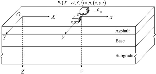
Theoretically, TSD tests of asphalt pavements can be simulated by a layered system subjected to a pair of uniformly moving constant rectangular surface loads. The asphalt layer in asphalt pavements is considered to be viscoelastic, while other components are considered to be elastic with hysteretic damping. In order to deal with the problem described above, a stationary Cartesian coordinate system (OXYZ) which is fixed on the pavement with origin being located at the centre of the initial loading area is introduced. Furthermore, the TSD device always measures the response of points around the right rear wheel pair, so it is convenient to introduce a moving Cartesian coordinate system (oxyz) which follows the load with origin being located at the centre of the moving loading area. These two coordinate systems are illustrated in Figure 1, it is clear that the TSD measurements correspond to the response of a set of fixed points in the moving coordinate system. It is assumed that the load moves along the X-axis with a constant speed c and these two coordinate systems are coincident when time t equals to zero, then the following coordinate relationships hold: (1) $x=X-ct,y=Y,z=Z$(1)

Furthermore, the relationships between the partial derivatives are as follows for nonnegative integer n: (2) $\frac{{\mathrm{\partial }}^n}{\mathrm{\partial }{X}^n}=\frac{{\mathrm{\partial }}^n}{\mathrm{\partial }{x}^n},\frac{{\mathrm{\partial }}^n}{\mathrm{\partial }{Y}^n}=\frac{{\mathrm{\partial }}^n}{\mathrm{\partial }{y}^n},\frac{{\mathrm{\partial }}^n}{\mathrm{\partial }{Z}^n}=\frac{{\mathrm{\partial }}^n}{\mathrm{\partial }{z}^n}$(2) (3) $\frac{{\mathrm{\partial }}^n}{\mathrm{\partial }{t}^n}|{}_{\underset{\_}{\mathbf{X}}}={\left(\frac{\mathrm{\partial }}{\mathrm{\partial }t}-c\frac{\mathrm{\partial }}{\mathrm{\partial }x}\right)}^n|{}_{\underset{\_}{\mathbf{x}}}$(3) where $\underset{\_}{\mathbf{X}}={\left[\begin{array}{ccc}X& Y& Z\end{array}\right]}^{\mathrm{T}}$ is the stationary coordinate vector and $\underset{\_}{\mathbf{x}}={\left[\begin{array}{ccc}x& y& z\end{array}\right]}^{\mathrm{T}}$ is the moving coordinate vector. The subscripts ‘$\underset{\_}{\mathbf{X}}$’ and ‘$\underset{\_}{\mathbf{x}}$’ indicate that corresponding functions are expressed in the stationary coordinate system and the moving coordinate system, respectively.

In this paper, the following Fourier transform conventions are used: (4) $\tilde{f}\left(k_x,k_y,z,\omega \right)={\int }_{-\mathrm{\infty }}^{\mathrm{\infty }}{\int }_{-\mathrm{\infty }}^{\mathrm{\infty }}{\int }_{-\mathrm{\infty }}^{\mathrm{\infty }}f\left(x,y,z,t\right)e^{\mathrm{i}\left(k_{x}x+k_{y}y-\omega t\right)}dxdydt$(4) (5) $\begin{array}{rl}& f\left(x,y,z,t\right)\\ & =\frac{1}{{\left(2\pi \right)}^3}{\int }_{-\mathrm{\infty }}^{\mathrm{\infty }}{\int }_{-\mathrm{\infty }}^{\mathrm{\infty }}{\int }_{-\mathrm{\infty }}^{\mathrm{\infty }}\tilde{f}\left(k_x,k_y,z,\omega \right)e^{-\mathrm{i}\left(k_{x}x+k_{y}y-\omega t\right)}d{k}_{x}d{k}_{y}d\omega \end{array}$(5) in which i is the imaginary unit satisfying ${\mathrm{i}}^2=-1$, $k_x$ is the wavenumber in the x-direction, $k_y$ is the wavenumber in the y-direction, $\omega$ is the angular frequency, $f\left(x,y,z,t\right)$ is an arbitrary function in the space–time domain related to the moving coordinate system, and $\tilde{f}\left(k_x,k_y,z,\omega \right)$ is the corresponding function in the wavenumber-frequency domain related to the moving coordinate system.

2.1. Spectral element formulation for viscoelastic layered systems

For a homogeneous, isotropic, and linearly viscoelastic material, the equation of motion in the frequency domain related to the stationary coordinate system can be expressed as follows in the absence of body forces (Al-Khoury et al. 2002): (6) $\left[{\hat{\lambda }}_0\left(\omega \right)+{\hat{\mu }}_0\left(\omega \right)\right]{\mathrm{\nabla }}_0{\mathrm{\nabla }}_0\cdot \widehat{\underset{\_}{\mathbf{U}}}\left(\underset{\_}{\mathbf{X}},\omega \right)+{\hat{\mu }}_0\left(\omega \right){\mathrm{\nabla }}_0^2\widehat{\underset{\_}{\mathbf{U}}}\left(\underset{\_}{\mathbf{X}},\omega \right)+\rho {\omega }^2\widehat{\underset{\_}{\mathbf{U}}}\left(\underset{\_}{\mathbf{X}},\omega \right)=\underset{\_}{\mathbf{0}}$(6) where the ‘hat’ means these quantities are frequency domain representations, ${\mathrm{\nabla }}_0={\left[\begin{array}{ccc}{\displaystyle \frac{\mathrm{\partial }}{\mathrm{\partial }X}}& {\displaystyle \frac{\mathrm{\partial }}{\mathrm{\partial }Y}}& {\displaystyle \frac{\mathrm{\partial }}{\mathrm{\partial }Z}}\end{array}\right]}^{\mathrm{T}}$ is the Del operator, ${\mathrm{\nabla }}_0^2={\displaystyle \frac{{\mathrm{\partial }}^2}{\mathrm{\partial }{X}^2}+\frac{{\mathrm{\partial }}^2}{\mathrm{\partial }{Y}^2}+\frac{{\mathrm{\partial }}^2}{\mathrm{\partial }{Z}^2}}$ is the Laplacian operator, ${\hat{\lambda }}_0\left(\omega \right)$ and ${\hat{\mu }}_0\left(\omega \right)$ are the complex Lamé constants, $\rho$ is the density, and $\widehat{\underset{\_}{\mathbf{U}}}\left(\underset{\_}{\mathbf{X}},\omega \right)$ is the displacement vector.

In order to solve Equation (6), the Helmholtz decomposition of the displacement vector is used: (7) $\widehat{\underset{\_}{\mathbf{U}}}\left(\underset{\_}{\mathbf{X}},\omega \right)={\mathrm{\nabla }}_0\hat{\mathrm{\Phi }}\left(\underset{\_}{\mathbf{X}},\omega \right)+{\mathrm{\nabla }}_0\times \widehat{\underset{\_}{\mathbf{\Psi }}}\left(\underset{\_}{\mathbf{X}},\omega \right)$(7) in which $\hat{\mathrm{\Phi }}\left(\underset{\_}{\mathbf{X}},\omega \right)$ is a scalar potential related to the P-wave, while $\widehat{\underset{\_}{\mathbf{\Psi }}}\left(\underset{\_}{\mathbf{X}},\omega \right)$ is a vector potential related to the S-wave and satisfies the gauge condition ${\mathrm{\nabla }}_0\cdot \widehat{\underset{\_}{\mathbf{\Psi }}}\left(\underset{\_}{\mathbf{X}},\omega \right)=0$. After substituting Equation (7) into Equation (6), the following equation can be obtained by using the identities ${\mathrm{\nabla }}_0\cdot {\mathrm{\nabla }}_0\hat{\mathrm{\Phi }}\left(\underset{\_}{\mathbf{X}},\omega \right)={\mathrm{\nabla }}_0^2\hat{\mathrm{\Phi }}\left(\underset{\_}{\mathbf{X}},\omega \right)$ and ${\mathrm{\nabla }}_0\cdot {\mathrm{\nabla }}_0\times \widehat{\underset{\_}{\mathbf{\Psi }}}\left(\underset{\_}{\mathbf{X}},\omega \right)=0$, and exchanging the order of operations: (8) ${\mathrm{\nabla }}_0\left\{\left[{\hat{\lambda }}_0\left(\omega \right)+2{\hat{\mu }}_0\left(\omega \right)\right]{\mathrm{\nabla }}_0^2\hat{\mathrm{\Phi }}+\rho {\omega }^2\hat{\mathrm{\Phi }}\right\}+{\mathrm{\nabla }}_0\times \left[{\hat{\mu }}_0\left(\omega \right){\mathrm{\nabla }}_0^2\widehat{\underset{\_}{\mathbf{\Psi }}}+\rho {\omega }^2\widehat{\underset{\_}{\mathbf{\Psi }}}\right]=\underset{\_}{\mathbf{0}}$(8)

Equation (8) will be satisfied if the following equations hold: (9) $\left[{\hat{\lambda }}_0\left(\omega \right)+2{\hat{\mu }}_0\left(\omega \right)\right]{\mathrm{\nabla }}_0^2\hat{\mathrm{\Phi }}\left(\underset{\_}{\mathbf{X}},\omega \right)+\rho {\omega }^2\hat{\mathrm{\Phi }}\left(\underset{\_}{\mathbf{X}},\omega \right)=0$(9) (10) ${\hat{\mu }}_0\left(\omega \right){\mathrm{\nabla }}_0^2\widehat{\underset{\_}{\mathbf{\Psi }}}\left(\underset{\_}{\mathbf{X}},\omega \right)+\rho {\omega }^2\widehat{\underset{\_}{\mathbf{\Psi }}}\left(\underset{\_}{\mathbf{X}},\omega \right)=\underset{\_}{\mathbf{0}}$(10)

According to Equations (2)–(5), for the transformation from the frequency domain related to the stationary coordinate system to the wavenumber-frequency domain related to the moving coordinate system, the following replacements need to be introduced in the terms related to partial derivatives: (11) $\frac{\mathrm{\partial }}{\mathrm{\partial }X}\to -\mathrm{i}{k}_x,\frac{\mathrm{\partial }}{\mathrm{\partial }Y}\to -\mathrm{i}{k}_y,\frac{\mathrm{\partial }}{\mathrm{\partial }Z}\to \frac{\mathrm{\partial }}{\mathrm{\partial }z}$(11) (12) $\omega \to \omega +c{k}_x$(12)

Hence, Equations (9) and (10) can be written as follows in the wavenumber-frequency domain related to the moving coordinate system: (13) $\left[\tilde{\lambda }\left(k_x,\omega \right)+2\tilde{\mu }\left(k_x,\omega \right)\right]{\tilde{\mathrm{\nabla }}}^2\tilde{\phi }\left(k_x,k_y,z,\omega \right)+\rho \left(\omega +c{k}_x{)}^2\tilde{\phi }\right(k_x,k_y,z,\omega )=0$(13) (14) $\tilde{\mu }\left(k_x,\omega \right){\tilde{\mathrm{\nabla }}}^2\widetilde{\underset{\_}{\psi }}\left(k_x,k_y,z,\omega \right)+\rho \left(\omega +c{k}_x{)}^2\underset{\_}{\tilde{\mathbf{\Psi }}}\right(k_x,k_y,z,\omega )=\underset{\_}{\mathbf{0}}$(14) where ${\tilde{\mathrm{\nabla }}}^2={\displaystyle \frac{{\mathrm{\partial }}^2}{\mathrm{\partial }{z}^2}-k_x^2-k_y^2}$ is the corresponding quantity of the Laplacian operator, $\tilde{\lambda }\left(k_x,\omega \right)$ and $\tilde{\mu }\left(k_x,\omega \right)$ are the corresponding quantities of the complex Lamé constants, $\tilde{\phi }\left(k_x,k_y,z,\omega \right)$ and $\widetilde{\underset{\_}{\psi }}\left(k_x,k_y,z,\omega \right)$ are respectively the corresponding quantities of the scalar and vector potentials. The solutions of Equations (13) and (14) can be sought in the following forms: (15) $\tilde{\phi }\left(k_x,k_y,z,\omega \right)=A{e}^{-\mathrm{i}{k}_{\mathrm{P}z}z}$(15) (16) $\underset{\_}{\tilde{\mathbf{\Psi }}}\left(k_x,k_y,z,\omega \right)={\left[\begin{array}{ccc}B& C& D\end{array}\right]}^{\mathrm{T}}{e}^{-\mathrm{i}{k}_{\mathrm{S}z}z}$(16) in which A, B, C, D are unknown coefficients to be determined by the boundary conditions, $k_{\mathrm{P}z}$ and $k_{\mathrm{S}z}$ are the wavenumbers in the z-direction of the P-wave and S-wave, respectively. It should be highlighted that the signs of $k_{\mathrm{P}z}$ and $k_{\mathrm{S}z}$ should be chosen carefully in accordance with the radiation condition for the case of the semi-infinite spectral element referred to below.

By substituting Equations (15) and (16) into Equations (13) and (14), the expressions of $k_{\mathrm{P}z}$ and $k_{\mathrm{S}z}$ are obtained: (17) $k_{\mathrm{P}z}^2=\frac{{\left(\omega +c{k}_x\right)}^2}{{\tilde{c}}_{\mathrm{P}}^2\left(k_x,\omega \right)}-k_x^2-k_y^2$(17) (18) $k_{\mathrm{S}z}^2=\frac{{\left(\omega +c{k}_x\right)}^2}{{\tilde{c}}_{\mathrm{S}}^2\left(k_x,\omega \right)}-k_x^2-k_y^2$(18) with ${\tilde{c}}_{\mathrm{P}}\left(k_x,\omega \right)=\sqrt{\left[\tilde{\lambda }\left(k_x,\omega \right)+2\tilde{\mu }\left(k_x,\omega \right)\right]/\rho }$ and ${\tilde{c}}_{\mathrm{S}}\left(k_x,\omega \right)=\sqrt{\tilde{\mu }\left(k_x,\omega \right)/\rho }$, which are related to the phase velocities of the P-wave and S-wave, respectively. In addition, by combining Equations (17) and (18) with the definitions of ${\tilde{c}}_{\mathrm{P}}\left(k_x,\omega \right)$ and ${\tilde{c}}_{\mathrm{S}}\left(k_x,\omega \right)$, the complex Lamé constants can be found to have the following relationship in the wavenumber-frequency domain: (19) $\tilde{\lambda }\left(k_x,\omega \right)=-\frac{k_x^2+k_y^2+2k_{\mathrm{P}z}^2-k_{\mathrm{S}z}^2}{k_x^2+k_y^2+k_{\mathrm{P}z}^2}\tilde{\mu }\left(k_x,\omega \right)$(19) Then, by following the same procedure as that for elastic layered systems shown in Sun et al. (2019), a layer spectral element and a semi-infinite spectral element are developed for viscoelastic layered systems based on the Spectral Element Method (SEM). The detailed formulation of these two spectral elements for viscoelastic layered systems is omitted in this paper because of the similarity to that for elastic layered systems. These two spectral elements can respectively simulate a layer and a half-space, and combinations of them are able to simulate different viscoelastic layered systems.

2.2. Simulation of material damping

The asphalt layer in asphalt pavements exhibits typical frequency/temperature dependent viscoelastic behaviours, which can be numerically simulated by different viscoelastic models. In this paper, the viscoelastic behaviours of the asphalt layer are simulated by the so-called 2S2P1D model (Olard and Di Benedetto 2003). This model consists of 2 spring elements, 2 parabolic elements, and 1 dashpot element, as shown in Figure 2.

Figure 2. Schematic representation of the 2S2P1D model.

The expression of the complex Young’s modulus of the 2S2P1D model in the frequency domain related to the stationary coordinate system has been presented in Olard and Di Benedetto (2003). With considering Equation (12), the complex Young’s modulus of the 2S2P1D model has the following expression in the wavenumber-frequency domain related to the moving coordinate system: (20) $\tilde{E}\left(k_x,\omega \right)=E_0+\left(E_{\mathrm{\infty }}-E_0\right)\left(\frac{{\kappa }_1}{{\kappa }_1^2+{\kappa }_2^2}+\mathrm{i}\frac{{\kappa }_2}{{\kappa }_1^2+{\kappa }_2^2}\right)$(20) where $\tilde{E}\left(k_x,\omega \right)$ is the complex Young’s modulus, and the definitions of ${\kappa }_1$ and ${\kappa }_2$ are: ${\kappa }_1=1+\zeta [\left(\omega +c{k}_x\right)\tau {]}^{-k}\cos \left(\frac{k\pi }{2}\right)+[\left(\omega +c{k}_x\right)\tau {]}^{-h}\cos \left(\frac{h\pi }{2}\right)$ ${\kappa }_2=\zeta [\left(\omega +c{k}_x\right)\tau {]}^{-k}\sin \left(\frac{k\pi }{2}\right)+[\left(\omega +c{k}_x\right)\tau {]}^{-h}\sin \left(\frac{h\pi }{2}\right)+[\text{β}\left(\omega +c{k}_x\right)\tau {]}^{-1}$in which $E_0$ is the static modulus obtained when $\omega \to 0$ ($E_0$ can be set to zero for binders), $E_{\mathrm{\infty }}$ is the glassy modulus obtained when $\omega \to \mathrm{\infty }$, $k$ and $h$ are dimensionless exponents of the two parabolic elements with relationship $0<k<h<1$, $\zeta$ is a positive dimensionless constant, $\tau$ is the characteristic time that depends only on temperature, and $\text{β}$ is a dimensionless constant which is related to the Newtonian viscosity $\eta$ of the dashpot via $\eta =\text{β}\tau \left(E_{\mathrm{\infty }}-E_0\right)$.

Other layers in asphalt pavements are generally composed of granular materials, which exhibit the so-called hysteretic damping (Sousa and Monismith 1987). For this kind of damping, the energy loss only depends on the path of a given motion. The complex Young’s modulus of such materials has the following expression in the wavenumber-frequency domain: (21) $\tilde{E}\left(k_x,\omega \right)=E\left[1+2\mathrm{i}\xi \mathrm{sgn}\left(\omega +c{k}_x\right)\right]$(21) where $E$ is the Young’s modulus, $\xi$ is the damping ratio, and $\mathrm{sgn}(\cdot )$ is the signum function.

For viscoelastic materials, the Poisson’s ratio could also be frequency/temperature dependent (Graziani et al. 2014). However, assuming a constant Poisson’s ratio still simulates the viscoelastic behaviours reasonably well, and it simplifies the simulation significantly. Therefore, it is assumed that each layer of asphalt pavements has a constant Poisson’s ratio. Consequently, the complex Lamé constants can be expressed as follows in the wavenumber-frequency domain: (22) $\tilde{\lambda }\left(k_x,\omega \right)=\frac{\nu \tilde{E}\left(k_x,\omega \right)}{\left(1+\nu \right)\left(1-2\nu \right)}$(22) (23) $\tilde{\mu }\left(k_x,\omega \right)=\frac{\tilde{E}\left(k_x,\omega \right)}{2\left(1+\nu \right)}$(23) in which $\nu$ is the Poisson’s ratio.

2.3. Simulation of TSD loading

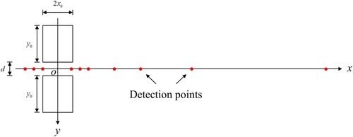
The TSD device can measure the vertical velocities of different points on the pavement surface by Doppler lasers mounted on a steel beam along the midline of the right rear wheel pair, and the positions of the detection points are shown in Figure 3. By combining the measured vertical velocities of these points with the driving speed, corresponding slopes of vertical deflection can be calculated. In reality, the contact area between the TSD wheel pair and the pavement surface is not regular, and the contact pressure is not uniform. However, to reasonably simplify the simulation, it is assumed that the contact area is rectangular and the contact pressure is uniform. The simulated TSD loading configuration used in this study is shown in Figure 3, which is in correspondence with the actual TSD loading configuration presented in Nasimifar et al. (2017).

Figure 3. Simulated TSD loading configuration.

In the moving coordinate system, the load applied by the TSD device can be expressed as follows: (24) $p_z\left(x,y,t\right)=h_0\left(x,y\right)p\left(t\right)$(24) where $p_z\left(x,y,t\right)$ is the load applied in the positive z-direction with dimension of force/area, $h_0\left(x,y\right)$ is the spatial distribution function of the load without dimension, and $p\left(t\right)$ is the loading history function with dimension of force/area. In order to describe the loading area shown in Figure 3, the spatial distribution function can be expressed as follows: (25) $\begin{array}{rl}& h_0\left(x,y\right)=\\ & H\left(x_0-\left|x\right|\right)\left[H\left(\frac{y_0}{2}-\left|y+\frac{y_0+d}{2}\right|\right)+H\left(\frac{y_0}{2}-\left|y-\frac{y_0+d}{2}\right|\right)\right]\end{array}$(25) in which $H(\cdot )$ is the Heaviside step function, $2x_0$ is the length of one rectangular loading area in x-direction, $y_0$ is the length of one rectangular loading area in y-direction, and $d$ is the distance between two rectangular loading areas. In addition, it is assumed that the TSD device applies a constant force on constant areas, which makes the loading history function constant, i.e. $p\left(t\right)=p_0$.

In the wavenumber-frequency domain, Equation (24) has the following form: (26) ${\tilde{p}}_z\left(k_x,k_y,\omega \right)=2\pi p_0\delta \left(\omega \right)h_1\left(k_x\right)h_2\left(k_y\right)$(26) where $\delta (\cdot )$ is the Dirac delta function, and the expressions of $h_1\left(k_x\right)$ and $h_2\left(k_y\right)$ are as follows: (27) $h_1\left(k_x\right)=\left\{\begin{array}{c}\frac{2\sin \left(k_x{x}_0\right)}{k_x},k_x\ne 0\\ 2x_0,k_x=0\end{array}\right.$(27) (28) $h_2\left(k_y\right)=\left\{\begin{array}{c}\frac{2}{k_y}\left\{\sin \left[\frac{k_y\left(2y_0+d\right)}{2}\right]-\sin \left(\frac{k_{y}d}{2}\right)\right\},k_y\ne 0\\ 2y_0,k_y=0\end{array}\right.$(28)

2.4. Solution procedure

In order to calculate the response of layered systems subjected to moving loads, the following steps are performed:

1. In the wavenumber-frequency domain, assemble the element stiffness matrices of all the spectral elements to obtain the system stiffness matrix;

2. Apply boundary conditions to calculate the nodal displacements, which are further used to compute the response fields within a certain spectral element;

3. Conduct inverse Fourier transform to obtain the response fields within this spectral element in the space–time domain.

In the inverse Fourier transform process, the integral with respect to $\omega$ is first evaluated analytically by using the property of the Dirac delta function, then the integrals with respect to $k_x$ and $k_y$ are discretised into summations to calculate the response fields in the space–time domain. The wavenumbers in the x-direction and y-direction are discretised with increments $\mathrm{\Delta }{k}_x=\pi /X_0$ and $\mathrm{\Delta }{k}_y=\pi /Y_0$, respectively. Parameters $2X_0$ and $2Y_0$ are the dimensions of a rectangular space window in the x-direction and y-direction, respectively. The space window has a centre located at the origin of the moving coordinate system, and its dimensions are large enough to ensure that the response outside the space window is negligible.

Actually, for a structure subjected to a moving constant load, the response in the moving coordinate system is constant over time. In other words, a moving constant load generates ‘frozen’ response fields which follow the load.

3. Model performance

In order to have an insight into the performance of the presented model, a case study is conducted in this section. The response of an asphalt pavement caused by a uniformly moving constant TSD load is considered. According to the actual loading conditions, the following parameters are used to represent the TSD load:

• The speed of movement $c=13.9\mathrm{m}/\mathrm{s}\left(50\mathrm{k}\mathrm{m}/\mathrm{h}\right);$

• The loading pressure $p_0=707\mathrm{k}\mathrm{P}\mathrm{a};$

• The distance between two rectangular loading areas $d=0.15\mathrm{m};$

• The parameters of the loading area $x_0=0.06316\mathrm{m}\mathrm{a}\mathrm{n}\mathrm{d}{y}_0=0.27432\mathrm{m};$

• The parameters of the space window $X_0=Y_0=200\mathrm{m}.$

The rear axle of the TSD device is loaded with 10 tonnes. With the parameter combination shown above, the total force $F_0$ used in the simulation is about 49 kN, which is comparable to the force applied by the right rear wheel pair of the TSD device. In addition, $4096\times 4096$ wavenumbers are consistently used in this paper to obtain converged results. The structural parameters of the asphalt pavement are shown in Table 1.

Table 1. Structural parameters of the asphalt pavement.

Layers	E	ξ	ν	ρ	l
	MPa	–	–	kg/m^3	m
Asphalt	–	–	0.3	2400	0.1
Base	500	0.05	0.3	2000	0.3
Subgrade	60	0.05	0.3	1600	Infinite

Note: E is the Young’s modulus, ξ is the damping ratio, ν is the Poisson’s ratio, ρ is the density, and l is the thickness.

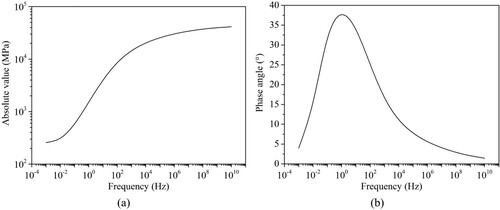
The complex Young’s modulus of the asphalt layer is simulated by the 2S2P1D model, which has the following parameters to represent an asphalt mixture labelled as ‘50/70 mix’ in Olard and Di Benedetto (2003): $E_0=250\mathrm{M}\mathrm{P}\mathrm{a}$, $E_{\mathrm{\infty }}=45400\mathrm{M}\mathrm{P}\mathrm{a}$, $k=0.175$, $h=0.55$, $\zeta =2.0$, $\text{β}=320$, and $\tau =3.855\times {10}^{-4}\mathrm{s}$ (at 25 degrees Celsius). With this parameter combination, the absolute value and phase angle of the complex Young’s modulus in the stationary coordinate system versus frequency are obtained, as shown in Figure 4.

Figure 4. Simulated complex Young’s modulus versus frequency: (a) absolute value, (b) phase angle.

3.1. Characteristics of model response

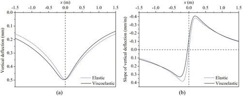
In this part, the performance of the presented model is demonstrated by investigating the characteristics of the model response. For the asphalt pavement with the specified loading and structural configuration, the vertical deflection curve and corresponding slope curve along the x-axis observed on the pavement surface are shown in Figure 5. These results are compared with those of a purely elastic model, in which the Young’s modulus of the asphalt layer is set to 3000 MPa and all the damping ratios are set to zero. The results indicate that the vertical deflection curve of the elastic layered system is totally symmetric and the maximum deflection appears at the centre of the loading area. However, for the viscoelastic layered system, the vertical deflection curve is slightly asymmetric and the maximum deflection appears behind the centre of the loading area. Compared with the case of the elastic layered system, the vertical deflection curve of the viscoelastic layered system increases more slowly after the load and decreases more quickly before the load with increasing x, which is also obvious from the slope curve. These conclusions are consistent with those shown in Nielsen (2019).

Figure 5. Comparison between the results of elastic and viscoelastic models: (a) vertical deflection curve, (b) slope curve of vertical deflection.

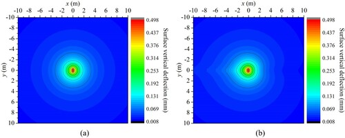
To have an insight into the surface deflection basin, the contour curves of surface vertical deflection for both the elastic and viscoelastic models are shown in Figure 6. The results indicate that the contour curves of surface vertical deflection for the elastic layered system are symmetric with respect to both y = 0 and x = 0. Hence, the surface deflection basin of the elastic layered system decreases at the same rate before and after the load. However, for the viscoelastic layered system, the contour curves of surface vertical deflection are only symmetric with respect to y = 0, while they are asymmetric with respect to x = 0. Specifically, the surface deflection basin of the viscoelastic layered system decreases more quickly before the load than after the load.

Figure 6. Contour curves of surface vertical deflection for different models: (a) elastic model, (b) viscoelastic model.

3.2. Comparison of model response

In this part, the performance of the presented Spectral Element Method-based (SEM-based) model is validated by comparing the response calculated by this model with that calculated by a Finite Element Method-based (FEM-based) model (Scarpas 1993). For convenience of calculation, the base layer is considered to be purely elastic and the subgrade is considered to be a purely elastic layer with a thickness of 5.0 m, while other loading and structural parameters remain the same.

The surface vertical deflection curves calculated by the two models are shown in Figure 7, which shows that the results calculated by different models have good agreement. The relative error of the maximum deflection is only 6.8%, which is acceptable considering different methodologies used in the two models. In addition, the computational requirements for different models are summarised in Table 2. The comparison indicates that the SEM-based model needs much less time and resource than the FEM-based model while giving relatively similar results. Hence, with considering the relatively high computational efficiency, the SEM-based model has the potential to be used as the computational kernel for parameter back-calculation procedures based on TSD measurements.

Figure 7. Comparison of vertical deflection curves calculated by different models.

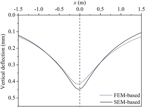
Table 2. Computational requirements for different models.

Models	Number of elements	Computational time	Number of processors	Type of processors
FEM-based	91800	4 h	32	Intel Xeon E5-2620 @ 2.40 GHz
SEM-based	3	2 min	8	Intel i7-7700HQ @ 2.80 GHz

4. Parameter sensitivity analysis

In this section, the sensitivity of the slope curve of vertical deflection along the x-axis observed on the surface of asphalt pavements to different parameters is investigated by conducting the single factor analysis. The loading and structural configuration presented in Section 3 is considered as a reference, the results of which are shown in solid lines. In the following analysis, the variation of a certain parameter is 50% of its reference value. In addition, for the convenience of description, the sensitivity of the slope curve to different parameters is qualitatively categorised into five levels: hardly sensitive, slightly sensitive, moderately sensitive, relatively sensitive, and highly sensitive.

4.1. Sensitivity to loading parameters

The sensitivity of the slope curve of vertical deflection to different loading parameters is researched in this part.

4.1.1. Magnitude of force

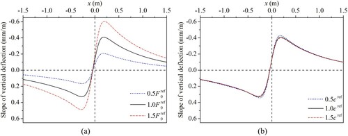
The slope curves of vertical deflection caused by a moving constant load with different magnitudes of force are presented in Figure 8(a). The variation of the magnitude of force is achieved by changing the loading area. The results show that the slope curve is highly sensitive to the magnitude of force. In addition, the results also indicate that, if the magnitude of force is greater, the vertical deflection curve will increase more quickly after the load and decrease more quickly before the load with increasing x.

Figure 8. Sensitivity of the slope curve of vertical deflection to loading parameters: (a) magnitude of force, (b) speed of movement.

4.1.2. Speed of movement

The slope curves of vertical deflection caused by a constant load with different speeds of movement are presented in Figure 8(b). The results show that the slope curve is moderately sensitive to the speed of movement, especially around the extrema.

4.2. Sensitivity to parameters of the 2S2P1D model

The sensitivity of the slope curve of vertical deflection to the parameters of the 2S2P1D model is studied in this part.

4.2.1. Static modulus

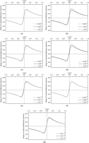
If the asphalt layer is simulated by the 2S2P1D model with different static moduli, the slope curves of vertical deflection as presented in Figure 9(a) are obtained. It can be seen that the results are almost identical, which means the slope curve is hardly sensitive to the static modulus.

Figure 9. Sensitivity of the slope curve of vertical deflection to parameters of the 2S2P1D model: (a) static modulus, (b) glassy modulus, (c) exponent k, (d) exponent h, (e) constant ζ, (f) constant β, (g) characteristic time.

4.2.2. Glassy modulus

If the asphalt layer is simulated by the 2S2P1D model with different glassy moduli, the slope curves of vertical deflection as presented in Figure 9(b) are obtained. The results show that the slope curve is relatively sensitive to the glassy modulus.

4.2.3. Exponent k

If the asphalt layer is simulated by the 2S2P1D model with different values of exponent k, the slope curves of vertical deflection as presented in Figure 9(c) are obtained. The results show that the slope curve is slightly sensitive to the exponent k.

4.2.4. Exponent h

If the asphalt layer is simulated by the 2S2P1D model with different values of exponent h, the slope curves of vertical deflection as presented in Figure 9(d) are obtained. The results show that the slope curve is relatively sensitive to the exponent h.

4.2.5. Constant ζ

If the asphalt layer is simulated by the 2S2P1D model with different values of constant ζ, the slope curves of vertical deflection as presented in Figure 9(e) are obtained. The results show that the slope curve is slightly sensitive to the constant ζ.

4.2.6. Constant β

If the asphalt layer is simulated by the 2S2P1D model with different values of constant β, the slope curves of vertical deflection as presented in Figure 9(f) are obtained. It can be seen that the results are almost identical, which means the slope curve is hardly sensitive to the constant β.

4.2.7. Characteristic time

If the asphalt layer is simulated by the 2S2P1D model with different values of characteristic time, the slope curves of vertical deflection as presented in Figure 9(g) are obtained. The results show that the slope curve is moderately sensitive to the characteristic time.

4.3. Sensitivity to structural parameters

The sensitivity of the slope curve of vertical deflection to different structural parameters is investigated in this part. In the legends of Figure 10, the subscripts ‘1’, ‘2’, and ‘3’ correspond to the asphalt layer, base layer, and subgrade, respectively

Figure 10. Sensitivity of the slope curve of vertical deflection to structural parameters: (a) Young’s modulus of base layer, (b) Young’s modulus of subgrade, (c) damping ratio of base layer, (d) damping ratio of subgrade, (e) Poisson’s ratio of asphalt layer, (f) Poisson’s ratio of base layer, (g) Poisson’s ratio of subgrade, (h) density of asphalt layer, (i) density of base layer, (j) density of subgrade, (k) thickness of asphalt layer, (l) thickness of base layer.

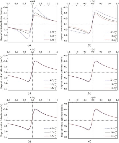
Figure 10. Continued.

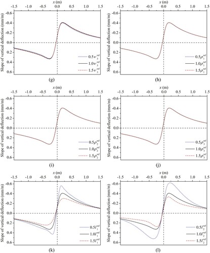
4.3.1. Young’s modulus

The slope curves of vertical deflection for asphalt pavements with different Young’s moduli of the base layer and subgrade are presented in Figure 10(a,b), respectively. The results show that the slope curve is highly sensitive to these two Young’s moduli, and the Young’s modulus of subgrade influences the response in a larger area than that of base layer.

4.3.2. Damping ratio

The slope curves of vertical deflection for asphalt pavements with different damping ratios of the base layer and subgrade are presented in Figure 10(c,d), respectively. The results show that the slope curve is slightly sensitive to these two damping ratios, and it is a bit more sensitive to the damping ratio of subgrade. In addition, it can also be concluded that the vertical deflection curve will be more asymmetric with increasing damping ratio.

4.3.3. Poisson’s ratio

The slope curves of vertical deflection for asphalt pavements with different Poisson’s ratios of the asphalt layer, base layer, and subgrade are presented in Figure 10(e–g), respectively. The results show that the slope curve is slightly sensitive to the Poisson’s ratios of the asphalt layer and subgrade, while it is moderately sensitive to the Poisson’s ratio of the base layer.

4.3.4. Density

The slope curves of vertical deflection for asphalt pavements with different densities of the asphalt layer, base layer, and subgrade are presented in Figure 10(h–j), respectively. It can be seen that the results are almost identical, which means the slope curve is hardly sensitive to all the densities.

4.3.5. Thickness

The slope curves of vertical deflection for asphalt pavements with different thicknesses of the asphalt layer and base layer are presented in Figure 10(k,l), respectively. The results show that the slope curve is highly sensitive to these two thicknesses.

5. Conclusions

This paper presents the formulation and application of a nonlinear spectral element model for the simulation of TSD tests of asphalt pavements. This model properly simulates the viscous damping in the asphalt layer (via the so-called 2S2P1D model) and the hysteretic damping in other layers. The spectral element model was used to demonstrate the differences between the response of elastic and viscoelastic layered systems under a pair of moving constant surface loads. In addition, the sensitivity of the slope curve of vertical deflection to different parameters was also investigated. On the basis of the discussions shown in this paper, the following conclusions can be drawn:

1. The vertical deflection curve along the x-axis observed on the surface of elastic layered systems is totally symmetric and the maximum deflection appears at the centre of the loading area. However, for viscoelastic layered systems, the vertical deflection curve is slightly asymmetric and the maximum deflection appears behind the centre of the loading area.

2. The slope curve of vertical deflection is highly sensitive to the magnitude of the applied force, the moduli of the base layer and subgrade, and the thicknesses of the asphalt layer and base layer. However, it is hardly sensitive to all the densities, the static modulus of the asphalt layer, and the constant β of the 2S2P1D model.

3. The slope curve of vertical deflection is relatively sensitive to the glassy modulus of the asphalt layer and the exponent h of the 2S2P1D model. It is moderately sensitive to the speed of movement, the Poisson’s ratio of the base layer, and the characteristic time of the 2S2P1D model. In addition, it is slightly sensitive to the damping ratios of the base layer and subgrade, the Poisson’s ratios of the asphalt layer and subgrade, and the exponent k and constant ζ of the 2S2P1D model.

The presented work gives a clear understanding of the mechanical mechanism, response characteristics, and response parameter sensitivity for TSD tests of asphalt pavements. In addition, the comparison with a finite element model shows that the proposed spectral element model has good predictive capability and high computational efficiency, so it has the potential to be used as the computational kernel for parameter back-calculation procedures based on TSD measurements.

6. Recommendations

The response of points around the right rear wheel pair of the TSD device could be affected by other wheel pairs. In the future work, it is recommended to consider the whole loading configuration of the TSD device to make the presented model even more realistic.

Acknowledgements

The first author would like to thank the financial support from the China Scholarship Council.

Disclosure statement

No potential conflict of interest was reported by the author(s).

Correction Statement

This article has been republished with minor changes. These changes do not impact the academic content of the article.

Additional information

Funding

This work was supported by the China Scholarship Council [grant number: 201608230114].

References

- Al-Khoury, R., et al., 2001a. Spectral element technique for efficient parameter identification of layered media. Part I: forward calculation. International Journal of Solids and Structures, 38 (9), 1605–1623. doi: https://doi.org/10.1016/S0020-7683(00)00112-8
- Al-Khoury, R., et al., 2001b. Spectral element technique for efficient parameter identification of layered media. Part II: inverse calculation. International Journal of Solids and Structures, 38 (48-49), 8753–8772. doi: https://doi.org/10.1016/S0020-7683(01)00109-3
- Al-Khoury, R., et al., 2002. Spectral element technique for efficient parameter identification of layered media. Part III: viscoelastic aspects. International Journal of Solids and Structures, 39 (8), 2189–2201. doi: https://doi.org/10.1016/S0020-7683(02)00079-3
- Chatti, K., et al., 2017. Enhanced analysis of falling weight deflectometer data for use with mechanistic-empirical flexible pavement design and analysis and recommendations for improvements to falling weight deflectometers. McLean, VA: Federal Highway Administration (FHWA). Publication No. FHWA-HRT-15-063.
- Graziani, A., Bocci, M., and Canestrari, F., 2014. Complex Poisson’s ratio of bituminous mixtures: measurement and modeling. Materials and Structures, 47 (7), 1131–1148. doi: https://doi.org/10.1617/s11527-013-0117-2
- Lee, H.S., Ayyala, D., and Von Quintus, H., 2017. Dynamic backcalculation of viscoelastic asphalt properties and master curve construction. Transportation Research Record: Journal of the Transportation Research Board, 2641 (1), 29–38. doi: https://doi.org/10.3141/2641-05
- Levenberg, E., et al., 2018. Comparing traffic speed deflectometer and falling weight deflectometer data. Transportation Research Record: Journal of the Transportation Research Board, 2672 (40), 22–31. doi: https://doi.org/10.1177/0361198118768524
- Li, M. and Wang, H., 2019. Development of ANN-GA program for backcalculation of pavement moduli under FWD testing with viscoelastic and nonlinear parameters. International Journal of Pavement Engineering, 20 (4), 490–498. doi: https://doi.org/10.1080/10298436.2017.1309197
- Maser, K., et al., 2017. Integration of traffic speed deflectometer and ground-penetrating radar for network-level roadway structure evaluation. Transportation Research Record: Journal of the Transportation Research Board, 2639 (1), 55–63. doi: https://doi.org/10.3141/2639-08
- Nasimifar, M., et al., 2016. Robust deflection indices from traffic-speed deflectometer measurements to predict critical pavement responses for network-level pavement management system application. Journal of Transportation Engineering, 142 (3), 04016004. doi: https://doi.org/10.1061/(ASCE)TE.1943-5436.0000832
- Nasimifar, M., Thyagarajan, S., and Sivaneswaran, N., 2017. Backcalculation of flexible pavement layer moduli from traffic speed deflectometer data. Transportation Research Record: Journal of the Transportation Research Board, 2641 (1), 66–74. doi: https://doi.org/10.3141/2641-09
- Nielsen, C.P., 2019. Visco-elastic back-calculation of traffic speed deflectometer measurements. Transportation Research Record: Journal of the Transportation Research Board, 2673 (12), 439–448. doi: https://doi.org/10.1177/0361198118823500
- Nobakht, M., et al., 2018. Mechanistic-empirical methodology for the selection of cost-effective rehabilitation strategy for flexible pavements. International Journal of Pavement Engineering, 19 (8), 675–684. doi: https://doi.org/10.1080/10298436.2016.1199878
- Nobakht, M., Sakhaeifar, M.S., and Newcomb, D., 2016. Development of rehabilitation strategies based on structural capacity for composite and flexible pavements. Journal of Transportation Engineering, Part A: Systems, 143 (4), 04016016. doi: https://doi.org/10.1061/JTEPBS.0000012
- Olard, F. and Di Benedetto, H., 2003. General “2S2P1D” model and relation between the linear viscoelastic behaviours of bituminous binders and mixes. Road Materials and Pavement Design, 4 (2), 185–224.
- Rada, G.R., et al., 2016. Pavement structural evaluation at the network level. McLean, VA: Federal Highway Administration (FHWA). Publication No. FHWA-HRT-15-074.
- Reddy, M.A., Reddy, K.S., and Pandey, B.B., 2014. Evaluation of rehabilitated urban recycled asphalt pavement. Road Materials and Pavement Design, 15 (2), 434–445. doi: https://doi.org/10.1080/14680629.2013.876924
- Roddis, W.M., Maser, K., and Gisi, A.J., 1992. Radar pavement thickness evaluations for varying base conditions. Transportation Research Record: Journal of the Transportation Research Board, 1355, 90–98.
- Scarpas, A., 1993. CAPA-3D finite elements system user’s manual: Parts I, II, and III. Delft, The Netherlands: Section of Structural Mechanics, Faculty of Civil Engineering and Geosciences, Delft University of Technology.
- Sousa, J.B. and Monismith, C.L., 1987. Dynamic response of paving materials. Transportation Research Record: Journal of the Transportation Research Board, 1136, 57–68.
- Sun, Z., et al., 2019. Dynamic analysis of layered systems under a moving harmonic rectangular load based on the spectral element method. International Journal of Solids and Structures, 180-181, 45–61. doi: https://doi.org/10.1016/j.ijsolstr.2019.06.022
- Uddin Ahmed Zihan, Z., et al., 2018. Development of a structural capacity prediction model based on traffic speed deflectometer measurements. Transportation Research Record: Journal of the Transportation Research Board, 2672 (40), 315–325. doi: https://doi.org/10.1177/0361198118758058
- Yang, Q. and Deng, Y., 2019. Evaluation of cracking in asphalt pavement with stabilized base course based on statistical pattern recognition. International Journal of Pavement Engineering, 20 (4), 417–424. doi: https://doi.org/10.1080/10298436.2017.1299528