Multiscale model for predicting freeze-thaw damage in asphalt mixtures

ABSTRACT

Freeze-thaw cycles in combination with long-term moisture exposure and traffic is a major threat to the performance of asphalt pavements. To enable characterisation and understanding of the damage process, this paper presents a new thermodynamics-based multiscale model of freeze-thaw damage in asphalt mixtures which also accounts for the damage due to moisture and traffic. The developed model consists of a microscale and a macroscale and is thereby able to account for the effect of the different microscale material components on the homogenous macroscale damage development. Additionally, the model is able to account for the acceleration of freeze-thaw damage which occurs when moisture infiltrates a damaged pavement with an increased effective air void content between freeze-thaw cycles. The novelty of the model lies in the ability to simulate the in-time acceleration of damage, the combined deteriorating effect of freeze-thaw cycles, moisture and traffic, as well as the coupling of the two scales to enable accurate predictions and understanding of the damage evolution. These features are demonstrated through a set of parametric examples which demonstrate the importance of including the effect of long-term moisture exposure and freeze-thaw cycles as well as the coupling between the different damage modes.

KEYWORDS:

• Asphalt mixture
• freeze-thaw damage
• micro-mechanics
• moisture damage
• multiscale model
• thermodynamics

1. Introduction

In many countries, asphalt concrete is the most commonly used material on paved roads. Its porous composite structure, consisting of load-carrying large aggregates, bitumen which acts as a binder in the material, and finer particles which increase the stiffness of the binder, gives it a complex behaviour, which includes: heterogeneity, viscoelasticity and viscoplasticity, and susceptibility to both cohesive damage in the mastic (i.e. the binder and filler mix) and adhesive damage between the aggregates and the mastic. The bituminous phase makes the mixture behaviour extremely sensitive to temperature, resulting in viscous behaviour at high temperatures and a more brittle elastic behaviour at low temperatures. Additionally, the porosity allows moisture to infiltrate the material, making it prone to moisture damage as well as freeze-thaw damage when subjected to low (cyclic) temperatures.

Infiltration of moisture into the asphalt mixture by diffusion may lead to emulsification of the binder close to the surface (Varveri et al. 2015) as well as stripping at the mastic-aggregate interface (Kringos et al. 2008b). Additionally, in more open asphalt structures, the moisture might erode the asphalt as it flows through the air void system (Kringos et al. 2008b). These mechanisms all cause a deterioration of material and structural properties that increase the risk of freeze-thaw damage, which occurs as the moisture trapped inside the air voids expands as it freezes to ice. The cyclic pressure inside the material caused by the freeze-thaw cycle may also lead to damage in the form of erosion, micro-cracks and chemo-mechanically induced deterioration of the material properties, eventually leading to an increase in volumetric pore volume in the mixture (Xu et al. 2015). This effectively leads to an overall decrease of different properties of the mixture, such as its strength and stiffness (Feng et al. 2010, Si et al. 2014, Luo et al. 2017, Pan et al. 2017).

In order to minimise or prevent this freeze-thaw damage from happening, it is important to understand and to be able to characterise the damage development as well as being able to identify the dominant parameters. Considering the complex behaviour of asphalt and the complex mechanism of the damage which may also be affected by other mechanisms, this characterisation is difficult to do experimentally. Computational modelling is therefore an important tool in the effort towards a better understanding of the damage process and which changes in the material and maintenance actions that could minimise the damage. Larger scale works for asphalt include Yi et al. (2014) which accounted for the material deterioration by a damage variable described by a Weibull distribution. Thermodynamics-based models include the works by Zhang et al. (2021) where the freeze-thaw damage was seen as a fatigue-type of damage and coupled to plasticity, Lövqvist et al. (2020b) which coupled the freeze-thaw damage to the damage caused by other external forces, and Kringos and Liu (2004) where a multiphase model approach was used which included an extra strain term for the freezing expansion and a Hoffman fracture criterion for the damage. While these models are able to make reliable predictions of the damage evolution and its effect on the material behaviour, they do not give further insight in how the material components affect the damage evolution and which parameters might be the most dominant for the mechanism. For this purpose, microscale models can provide a better understanding. Such a model was developed by Varveri et al. (2014), where the temperature dependent extra strain due to freezing was included in the deformation tensor, and also accounted for the cohesive damage in the binder. Another microscale model was suggested in Lövqvist et al. (2021), which included the moisture infiltration, a temperature dependent strain inside the air voids, as well as coupled the moisture damage and freeze-thaw damage inside both the mastic (cohesive damage) and in the mastic-aggregate interface (adhesive damage).

However, even though these types of models can provide much useful information on the behaviour of the asphalt mixture and the damage mechanism, using them directly for an entire asphalt pavement is not feasible considering the very high number of degrees of freedom that would be required due to the complex microstructure and many potential damage locations. This would require a high computational power and time effort, which is not optimal for the purpose. The level of detail included in a microscale model is thus not suitable for simulations at the pavement scale. Furthermore, microscale models of asphalt microstructures are also not able to easily include effects of other mechanisms that occur on different scales or in different layers of the pavement, e.g. frost heave. To avoid these limitations, but still be able to use the information given from the microscale for the whole asphalt layer(s) in the pavement, multiscale modelling is a useful approach.

Multiscale models enable linking of separately run continuum mechanics simulations on different scales without losing a substantial amount of accuracy, under the condition that the two length scales are widely different (Allen 2001). This allows inclusion of the effects of different parameters on the smaller scale without requiring the inclusion of all microstructural details in the larger scale simulation, thus saving a substantial amount of computational effort and time. The dependency of the larger scale on the smaller scale can be achieved by performing analyses on a Representative Volume Element (RVE) on the smaller structural scale, which fulfils statistical homogeneity, in a macroscopic body and then utilising the homogenisation principle to determine the field equations for the larger scale. Only using this homogenisation principle to determine the material properties on the larger scale, such that the model is one-way coupled, is possible in the case that the RVE does not change during the simulation and the material behaviour is not history dependent. This type of one-way coupled model, which only predicts the behaviour of the larger scale based on the smaller scale once, can also be called a ‘bottom-up’ (Aigner et al. 2009) or ‘expanding’ (Allen et al. 2017a) multiscale model. In addition to being able to predict the material behaviour on the larger scale based on the material properties of the constituents (Aigner et al. 2009, Garcia Cucalon et al. 2016) and thereby saving effort on experimental testing, this type of multiscale models can also aid in understanding the role of different design variables and material properties on the smaller scale (Füssl and Lackner 2011, Allen et al. 2017a). Another type of one-way coupled models is ‘top-down’ or ‘contracting’ multiscale models, which can be utilised to predict the location, initiation and propagation of cracks on the smaller scale based on the design variables given by the larger scale (Allen et al. 2017b). In the case that the material behaviour is history dependent, the RVE experiences changes (e.g. cracking) or the boundary conditions are differed during the simulation, two-way coupled models are more suitable. The different scales (two or more) are then run simultaneously, with the larger scale controlling the boundary conditions or stresses of the local scale and the results from the smaller scale being homogenised to get the properties for the next time step of the larger scale (Souza et al. 2008, Lutif et al. 2010, Souza and Allen 2010, Teixeira et al. 2014, Allen et al. 2017c, Sun et al. 2019, Wollny et al. 2020). These multiscale models clearly show the advantages of multiscale models regarding the improvement of understanding of the effects of different material parameters, improved predictions, the saved computational effort and minimisation of experimental tests needed for calibration. Despite this, there is a lack of multiscale models which can concern the effect of environmental impact, such as freeze-thaw cycles, on asphalt materials.

1.1. Aim of paper

Despite the large problem of freeze-thaw damage in asphalt pavements in regions with cold and wet climates, there is a lack of models which can both predict the damage development and also aid in characterising the damage process and understanding the role of different parameters of the material constituents. This paper therefore aims to develop a new multiscale model of freeze-thaw damage in the asphalt layers of the pavement. The emphasis of the multiscale model lies on the damage evolution due to freeze-thaw cycles but also includes the effect of moisture and mechanical loading. As the aim is to develop a model which can be used to understand the role of different parameters on the damage evolution, the multiscale is of a bottom-up type and consists of two scales: a microscale consisting of mastic, aggregates and air voids, and a macroscale which treats the asphalt concrete as a homogenous material.

This paper first gives a description of the multiscale model as well as most of the details of the microscale and macroscale equations. This includes the equation for accounting for the effect of the overall increase of air voids on the evolution of the freeze-thaw damage on the macroscale in case the new air voids are filled with more moisture. Thereafter, the procedure for determining the damage parameters for the macroscale is presented, utilising a multiscale approach. Finally, the application of the model is presented by using a set of different weather scenarios for which the total damage evolution is predicted.

2. Model formulation

The purpose of the developed multiscale model presented herein is to obtain a deeper understanding of how different parameters on the scale of the material constituents affect the development of freeze-thaw damage in an asphalt pavement. For this reason, together with the requirement (1) $l^G\gg l^L$(1) where $l^G$ is the global length scale and $l^L$ the local length scale, the multiscale framework is chosen to consist of two scales: a local microscale, including the mastic, large aggregates and the air voids which can consist of either moisture or ice, and a global scale of the pavement. The local scale is a micromechanical model which includes the infiltration of moisture, the expansion of moisture inside the air voids due to freezing and a coupled damage depending on both the moisture and mechanical stresses. For the global scale of the asphalt pavement, a macroscale model of a homogenised asphalt mixture material is used, which includes the damage due to the internal stresses caused by the freeze-thaw cycles and the damage due to the energy caused by external forces acting on the material.

Considering the purpose of the multiscale model, the model is set up as a one-way coupled ‘bottom-up’ type model such that the global scale is affected by the local scale but not vice versa. However, as it has been shown that the air void content of the mixture affects the freeze-thaw damage evolution (Feng et al. 2010, Lövqvist et al. 2020a), it is important to account for the effect of an increasing air void content on the damage evolution. This effect is therefore included in the evolution of freeze-thaw damage on the macroscale. As the model focuses on the behaviour of the asphalt mixture at low temperatures, behaviours associated with higher temperatures, such as healing and (visco)plasticity, are neglected.

In the following sections, the equations for the two scales are briefly described. A more detailed description about the microscale model and macroscale model can be found in Lövqvist et al. (2020b, 2021), respectively. Both models are based on continuum mechanics and thermodynamics. For all following model descriptions, the notations x, $\mathit{x}$ and $\overline{\mathit{x}}$ stand for scalar and second- and fourth-order tensors, respectively, $(:)$ is the double contraction product, and $〈x〉$ are Macaulay brackets, i.e. $〈x〉=\frac{x+\left|x\right|}{2}$.

2.1. Effective configuration

Both scales utilise the concept of Continuum Damage Mechanics (CDM) (Kachanov 1958, Rabotnov 1969) to relate the effective undamaged state of a material to its nominal damaged one. In this concept, a damage variable, d, is introduced to represent the density of microcracks in the material and is only allowed to vary between 0, undamaged state, and 1, fully damaged state. In this work, an isotropic damage evolution is considered and the damage variable is then a scalar. Utilising the CDM concept, the effective stress $\tilde{\mathit{\sigma }}$ can be formulated as (2) $\tilde{\mathit{\sigma }}=\frac{\mathit{\sigma }}{1-d},$(2) where $\mathit{\sigma }$ is the nominal stress. Furthermore, both models assume that the free energy is equal in the effective and nominal configurations (energy equivalence hypothesis) such that (3) $\psi (\tilde{\mathit{\sigma }},\widetilde{\mathit{ϵ}})=\psi (\mathit{\sigma },\mathit{ϵ}),$(3) where the effective strain is (4) $\widetilde{\mathit{ϵ}}=(1-d)\mathit{ϵ}.$(4)

2.2. The microscale model

The micromechanical model used for the microscale consists of three parts: the moisture transportation, the expansion from moisture to ice, and the damage caused by both moisture and mechanical loading. The model considers a microstructure including larger aggregates, mastic and air voids. Damage can occur both inside the mastic itself (cohesive damage) and between the aggregates and the mastic (adhesive damage). The aggregates are assumed to have a linear elastic behaviour and the mastic to be viscoelastic.

2.2.1. Moisture transportation

To model the infiltration of moisture into the mastic from the surrounding environment and intrinsic air voids, Fick's second law is utilised (5) $\frac{\mathrm{\partial }{c}^L}{\mathrm{\partial }t}=D^L\frac{{\mathrm{\partial }}^2{c}^L}{\mathrm{\partial }{x}^2},$(5) in which c is the concentration of moisture, $D^L$ the diffusion coefficient, in this work assumed to be isotropic, and x the location. This work uses a normalised concentration such that (6) ${\theta }^L=\frac{c^L}{c_{max}^L},$(6) where $c_{max}^L$ is the maximum concentration in the air voids, thus changing Equation (5(5) $\frac{\mathrm{\partial }{c}^L}{\mathrm{\partial }t}=D^L\frac{{\mathrm{\partial }}^2{c}^L}{\mathrm{\partial }{x}^2},$(5) ) to (7) $\frac{\mathrm{\partial }{\theta }^L}{\mathrm{\partial }t}=D^L\frac{{\mathrm{\partial }}^2{\theta }^L}{\mathrm{\partial }{x}^2}.$(7) At the interfaces between the different material components (aggregates, mastic and air voids), continuity is assumed to apply such that (8) ${\theta }^{aggregates}={\theta }^{mastic}={\theta }^{voids}.$(8) To ensure that moisture only diffuses in the asphalt mixture at temperatures above the freezing point, in this work assumed as $0^{\circ }\mathrm{C}$, the diffusion coefficients are set as a function of temperature according to (9) $D^L\left(T\right)=D^L\frac{〈T_{freezing}-T〉}{T_{freezing}-T},$(9) where $T_{freezing}$ is the freezing temperature.

2.2.2. Expansion of ice

To model the stress in the air voids which occurs when they are filled with ice, the multi-phase formulation from Kringos and Liu (2004) is used (10) ${\mathit{\sigma }}^{L,voids}=(K^{ice}-\frac{2}{3}{G}^{ice})[\mathrm{t}\mathrm{r}({\mathit{ϵ}}^{L,voids})-\alpha |\mathrm{\Delta }T|-{ϵ}_{\varphi }]\mathit{I}+2G^{ice}{\mathit{ϵ}}^{L,voids},$(10) in which $K^{ice}$ and $G^{ice}$ are the bulk and shear modulus of the ice, respectively, ${\mathit{ϵ}}^{L,voids}$ the strain, $\mathrm{t}\mathrm{r}\left({\mathit{ϵ}}^{L,voids}\right)$ the volumetric strain, α the temperature expansion coefficient of ice, $\mathrm{\Delta }T$ the change in temperature, ${ϵ}_{\varphi }$ the strain occurring from the expansion from water to ice, and I the identity matrix. This work considers the expansion from water to ice to occur as purely volumetric and assumes that the temperature expansion coefficient of ice, α, is negligible compared to the strain occurring from the expansion from water to ice, ${ϵ}_{\varphi }$, of approximately 0.09 (e.g. Kringos and Liu 2004, Varveri et al. 2014, Lövqvist et al. 2021). Additionally, the bulk shear modulus of the ice and the ice expansion strain are assumed to depend on the temperature to account for the change of properties caused by the temperature changes, (11) $K^{ice}\left(T\right)=K^{ice}\frac{〈T_{freezing}-T〉}{T_{freezing}-T},$(11) (12) ${ϵ}_{\varphi }\left(T\right)={ϵ}_{\varphi }\frac{〈T_{freezing}-T〉}{T_{freezing}-T}.$(12) Equation (10(10) ${\mathit{\sigma }}^{L,voids}=(K^{ice}-\frac{2}{3}{G}^{ice})[\mathrm{t}\mathrm{r}({\mathit{ϵ}}^{L,voids})-\alpha |\mathrm{\Delta }T|-{ϵ}_{\varphi }]\mathit{I}+2G^{ice}{\mathit{ϵ}}^{L,voids},$(10) ) can thus be rewritten as (13) ${\mathit{\sigma }}^{L,voids}=K^{ice}[\mathrm{t}\mathrm{r}\left({\mathit{ϵ}}^{L,voids}\right)-{ϵ}_{\varphi }]\mathit{I}.$(13)

2.2.3. Mastic material model

The mastic is considered to be viscoelastic and is exposed to both mechanical damage, $d^{L,\mathrm{\Psi }}$, and moisture damage, $d^{L,\theta }$. In this work, it is assumed that moisture damage can occur inside the mastic (cohesive damage) and in the aggregate-mastic interface (adhesive damage) due to the existence of moisture inside the material components which deteriorates the strength of the material. Other moisture damage sources such as erosion and pumping action are disregarded in this model considering their different time scales compared to the freeze-thaw damage which is the focus of this work.

To couple the two types of damages such that both contribute to the total damage on the local scale, a multiplicative coupling approach is used (see, e.g. Kringos et al. 2008c, Shakiba et al. 2016) (14) $(1-d^L)=(1-d^{L,\theta })(1-d^{L,\mathrm{\Psi }}).$(14) The free energy of the mastic is therefore a function of the two damage variables, together with the viscoelastic strain and an internal variable $h^{L,\mathrm{\Psi }}$, related to the change in size of the mechanical damage surface, according to (15) ${\psi }^L={\psi }^L({\mathit{ϵ}}^L,{\mathit{ϵ}}_n^{L,v},d^{L,\theta },d^{L,\mathrm{\Psi }},h^{L,\mathrm{\Psi }}).$(15) The viscoelastic behaviour of the mastic is in this work described by using a Prony series of the Generalised Maxwell model, consisting of n terms. The total strain for a Maxwell element of the mastic ${\mathit{ϵ}}^L$ therefore consists of an elastic part, ${\mathit{ϵ}}^{L,e}$, and a viscous part, ${\mathit{ϵ}}_n^{L,v}$, such that (16) ${\mathit{ϵ}}^L={\mathit{ϵ}}_n^L={\mathit{ϵ}}_n^{L,e}+{\mathit{ϵ}}_n^{L,v}.$(16) The viscoelastic part of the free energy can also be decomposed into a long-term equilibrium part, ${\psi }^{L,\mathrm{\infty }}$, and a non-equilibrium part, ${\psi }_n^{L,v}$ according to the Generalised Maxwell model (17) ${\psi }^{L,ve}={\psi }^{L,\mathrm{\infty }}+\sum _{n=1}^N{\psi }_n^{L,v}.$(17) Considering Equation (4(4) $\widetilde{\mathit{ϵ}}=(1-d)\mathit{ϵ}.$(4) ), the two parts of the elastic free energy can be written as (18) ${\psi }^{L,\mathrm{\infty }}=(1-d^{L,\theta }{)}^2(1-d^{L,\mathrm{\Psi }}{)}^2\cdot \frac{1}{2}{\mathit{ϵ}}_n^L:{\mathit{E}}_{\mathrm{\infty }}^L:{\mathit{ϵ}}_n^L,$(18) (19) $\sum _{n=1}^N{\psi }_n^{L,v}=(1-d^{L,\theta }{)}^2(1-d^{L,\mathrm{\Psi }}{)}^2\cdot \frac{1}{2}\sum _{n=1}^N({\mathit{ϵ}}_n^L-{\mathit{ϵ}}_n^{L,v}):{\overline{\mathit{E}}}_n^L\left(t\right):({\mathit{ϵ}}_n^L-{\mathit{ϵ}}_n^{L,v}),$(19) where t is the time, ${\mathit{E}}_{\mathrm{\infty }}^L$ the long-term stiffness tensor, and ${\overline{\mathit{E}}}_n^L\left(t\right)$ the fourth-order stiffness tensor of the nth branch in the viscoelastic formulation, according to (20) ${\overline{\mathit{E}}}_n^L\left(t\right)={\overline{\mathit{E}}}_n^L\cdot \exp (-\frac{t}{{\tau }_n^L}),$(20) in which ${\tau }_n^L$ is the relaxation time of the nth branch. To account for the temperature dependent behaviour of the mastic, a William-Landel-Ferry (WLF) shift factor is used according to (21) $\log \left({\alpha }_T^L\right)=-\frac{C_1^L(T-T_{ref}^L)}{C_2+T-T_{ref}^L},$(21) where ${\alpha }_T^L$ is the shift factor, $C_1^L$ and $C_2^L$ empirical constants, T the temperature and $T_{ref}^L$ the reference temperature. The reduced time, $t_R$, is determined by using the shift factor such that (22) $t_R^L=\frac{t}{{\alpha }_T^L}.$(22) This gives the resulting Prony series for the stiffness of the mastic (23) ${\overline{\mathit{E}}}^L\left(T\right)={\overline{\mathit{E}}}_{\mathrm{\infty }}^L+\sum _{n=1}^N{\overline{\mathit{E}}}_n^L\exp (-\frac{t_R^L\cdot {\alpha }_T^L}{{\tau }_n^L}).$(23) The part of the free energy which describes the effect of an increase in size of the damage surface, similar to a hardening of the damage, is described by (24) ${\psi }^{L,h}=K_1[\frac{1}{K_2}\cdot \exp \left(K_2{h}^{L,\mathrm{\Psi }}\right)-h^{L,\mathrm{\Psi }}],$(24) in which $K_1$ and $K_2$ are material parameters. The total mastic free energy is thus (25) $\begin{array}{rl}{\psi }^L& ={\psi }^{L,ve}+{\psi }^{L,h}\\ & =\frac{1}{2}(1-d^{L,\theta }{)}^2(1-d^{L,\mathrm{\Psi }}{)}^2\cdot [{\mathit{ϵ}}_n^L:{\overline{\mathit{E}}}_{\mathrm{\infty }}^L:{\mathit{ϵ}}_n^L\phantom{\sum _{n=1}^N}\\ & +\sum _{n=1}^N({\mathit{ϵ}}_n^L-{\mathit{ϵ}}_n^{L,v}):{\overline{\mathit{E}}}_n^L\left(t\right):({\mathit{ϵ}}_n^L-{\mathit{ϵ}}_n^{L,v})]\\ & +K_1[\frac{1}{K_2}\cdot \exp \left(K_2{h}^{L,\mathrm{\Psi }}\right)-h^{L,\mathrm{\Psi }}].\end{array}$(25) By using the second law of thermodynamics and time differentiating the free energy, the Clausius–Duhem inequality equation for the local dissipation can be written as (26) $\frac{\mathrm{\partial }{\psi }^L}{{\mathit{ϵ}}^L}:{\mathit{ϵ}}^L-\frac{\mathrm{\partial }{\psi }^L}{\mathrm{\partial }{\mathit{ϵ}}_n^{L,v}}:{\dot{\mathit{ϵ}}}_n^{L,v}-\frac{\mathrm{\partial }{\psi }^L}{\mathrm{\partial }{d}^{L,\theta }}:{\dot{d}}^{L,\theta }-\frac{\mathrm{\partial }{\psi }^L}{\mathrm{\partial }{d}^{L,\mathrm{\Psi }}}:{\dot{d}}^{L,\mathrm{\Psi }}-\frac{\mathrm{\partial }{\psi }^L}{\mathrm{\partial }{h}^{L,\mathrm{\Psi }}}:{\dot{h}}^{L,\mathrm{\Psi }}\ge 0.$(26) The thermodynamic forces which are work-conjugated to the internal variables can thus be defined according to (27) ${\mathit{\sigma }}^L=\frac{\mathrm{\partial }{\psi }^L}{\mathrm{\partial }{\mathit{ϵ}}^L},$(27) (28) ${\mathit{\sigma }}_n^{L,v}=\frac{\mathrm{\partial }{\psi }^L}{\mathrm{\partial }{\mathit{ϵ}}_n^{L,v}},$(28) (29) $Y^{L,\theta }=-\frac{\mathrm{\partial }{\psi }^L}{\mathrm{\partial }{d}^{L,\theta }},$(29) (30) $Y^{L,\mathrm{\Psi }}=-\frac{\mathrm{\partial }{\psi }^L}{\mathrm{\partial }{d}^{L,\mathrm{\Psi }}},$(30) (31) $H^{L,\mathrm{\Psi }}=\frac{\mathrm{\partial }{\psi }^L}{\mathrm{\partial }{h}^{L,\mathrm{\Psi }}},$(31) where ${\mathit{\sigma }}^L$ is the stress in the mastic, ${\mathit{\sigma }}_n^{L,v}$ the viscous part of the stress in the mastic, $Y^{L,\theta }$ and $Y^{L,\mathrm{\Psi }}$ the moisture and mechanical damage strain energy release rates, respectively, and $H^{L,\mathrm{\Psi }}$ a generalised force related to the increase rate of the damage surface. The principle of maximum dissipation is used so that the dissipation potentials can be used to derive the evolution equations of the internal variables. In this work, a decomposed dissipation potential is used such that $F^L=F_n^{L,v}+F^{L,\theta }+F^{L,\mathrm{\Psi }}$, where $F_n^{L,v}$ is the viscoelastic dissipation, $F^{L,\theta }$ the dissipation due to moisture damage and $F^{L,\mathrm{\Psi }}$ the dissipation due to mechanical damage. Furthermore, this study assumes the case of associated damage laws for the mechanical damage such that $f^{L,\mathrm{\Psi }}=F^{L,\mathrm{\Psi }}$. This leads to the following derivations of the evolution equations: (32) ${\dot{\mathit{ϵ}}}_n^{L,v}=\frac{\mathrm{\partial }{F}_n^{L,v}}{\mathrm{\partial }{\mathit{\sigma }}_n^{L,v}},$(32) (33) ${\dot{d}}^{L,\theta }=\frac{\mathrm{\partial }{F}^{L,\theta }}{\mathrm{\partial }{Y}^{L,\theta }},$(33) (34) ${\dot{d}}^{L,\mathrm{\Psi }}=\frac{\mathrm{\partial }{F}^{L,\mathrm{\Psi }}}{\mathrm{\partial }{Y}^{L,\mathrm{\Psi }}}{\dot{\lambda }}^{L,\mathrm{\Psi }}=\frac{\mathrm{\partial }{f}^{L,\mathrm{\Psi }}}{\mathrm{\partial }{Y}^{L,\mathrm{\Psi }}}{\dot{\lambda }}^{L,\mathrm{\Psi }},$(34) (35) ${\dot{h}}^{L,\mathrm{\Psi }}=-\frac{\mathrm{\partial }{F}^{L,\mathrm{\Psi }}}{\mathrm{\partial }{H}^{L,\mathrm{\Psi }}}{\dot{\lambda }}^{L,\mathrm{\Psi }}=-\frac{\mathrm{\partial }{f}^{L,\mathrm{\Psi }}}{\mathrm{\partial }{H}^{L,\mathrm{\Psi }}}{\dot{\lambda }}^{L,\mathrm{\Psi }},$(35) where ${\dot{\lambda }}^{L,\mathrm{\Psi }}$ is a Lagrangian damage multiplier.

2.2.3.1. Viscoelasticity

The thermodynamic force work-conjugated to the viscous part of the strain is the viscous part of the stress according to (36) ${\mathit{\sigma }}_n^{L,v}=\frac{\mathrm{\partial }{\psi }^L}{\mathrm{\partial }{\mathit{ϵ}}_n^{L,v}}=(1-d^{L,\theta }{)}^2(1-d^{L,\mathrm{\Psi }}{)}^2\cdot \sum _{n=1}^N{\overline{\mathit{E}}}_n^L\left(t\right):({\mathit{ϵ}}_n^L-{\mathit{ϵ}}_n^{L,v}).$(36) The viscous part of the dissipation potential is defined as (Onifade et al. 2015) (37) $F_n^{L,v}=\frac{1}{2{\mu }_n^L}{\mathit{\sigma }}_n^{L,v}:{\mathit{\sigma }}_n^{L,v},$(37) where ${\mu }_n^L$ is the viscosity of the nth viscous component of the Generalised Maxwell model. Using Equation (32(32) ${\dot{\mathit{ϵ}}}_n^{L,v}=\frac{\mathrm{\partial }{F}_n^{L,v}}{\mathrm{\partial }{\mathit{\sigma }}_n^{L,v}},$(32) ), the evolution of the viscous part of the strain can thus be written as (38) ${\dot{\mathit{ϵ}}}_n^{L,v}=\frac{\mathrm{\partial }{F}_n^{L,v}}{\mathrm{\partial }{\mathit{\sigma }}_n^{L,v}}=\frac{1}{{\mu }_n^L}{\mathit{\sigma }}_n^{L,v}.$(38)

2.2.3.2. Moisture damage

The thermodynamic force which is work-conjugated to the moisture damage variable is derived according to Equation (29(29) $Y^{L,\theta }=-\frac{\mathrm{\partial }{\psi }^L}{\mathrm{\partial }{d}^{L,\theta }},$(29) ) such that (39) $\begin{array}{rl}{Y}^{L,\theta }=-\frac{\mathrm{\partial }{\psi }^L}{\mathrm{\partial }{d}^{L,\theta }}& =(1-d^{L,\theta })(1-d^{L,\mathrm{\Psi }}{)}^2\cdot [{\mathit{ϵ}}_n^L:{\overline{\mathit{E}}}_{\mathrm{\infty }}^L:{\mathit{ϵ}}_n^L\phantom{\sum _{n=1}^N}\\ & +\sum _{n=1}^N({\mathit{ϵ}}_n^L-{\mathit{ϵ}}_n^{L,v}):{\overline{\mathit{E}}}_n^L\left(t\right):({\mathit{ϵ}}_n^L-{\mathit{ϵ}}_n^{L,v})].\end{array}$(39) Remembering that $\begin{array}{rl}{\mathit{\sigma }}^L& =\frac{\mathrm{\partial }{\psi }^L}{\mathrm{\partial }{\mathit{ϵ}}^L}=(1-d^{L,\theta }{)}^2(1-d^{L,\mathrm{\Psi }}{)}^2\\ \left(40\right)& & \cdot [{\overline{\mathit{E}}}_{\mathrm{\infty }}^L:{\mathit{ϵ}}_n^L+\sum _{n=1}^N{\overline{\mathit{E}}}_n^L\left(t\right):({\mathit{ϵ}}_n^L-{\mathit{ϵ}}_n^{L,v})],\end{array}$Equation (39(39) $\begin{array}{rl}{Y}^{L,\theta }=-\frac{\mathrm{\partial }{\psi }^L}{\mathrm{\partial }{d}^{L,\theta }}& =(1-d^{L,\theta })(1-d^{L,\mathrm{\Psi }}{)}^2\cdot [{\mathit{ϵ}}_n^L:{\overline{\mathit{E}}}_{\mathrm{\infty }}^L:{\mathit{ϵ}}_n^L\phantom{\sum _{n=1}^N}\\ & +\sum _{n=1}^N({\mathit{ϵ}}_n^L-{\mathit{ϵ}}_n^{L,v}):{\overline{\mathit{E}}}_n^L\left(t\right):({\mathit{ϵ}}_n^L-{\mathit{ϵ}}_n^{L,v})].\end{array}$(39) ) can be rewritten as (41) $\begin{array}{rl}{Y}^{L,\theta }& =(1-d^{L,\theta })(1-d^{L,\mathrm{\Psi }}{)}^2\cdot [\frac{{\mathit{\sigma }}^{L,\mathrm{\infty }}}{(1-d^{L,\theta }{)}^2(1-d^{L,\mathrm{\Psi }}{)}^2}:{\mathit{ϵ}}_n^L\phantom{\sum _{n=1}^N}\\ & +\sum _{n=1}^N\frac{{\mathit{\sigma }}_n^{L,v}}{(1-d^{L,\theta }{)}^2(1-d^{L,\mathrm{\Psi }}{)}^2}:({\mathit{ϵ}}_n^L-{\mathit{ϵ}}_n^{L,v})]\\ & =\frac{{\mathit{\sigma }}^{L,\mathrm{\infty }}}{(1-d^{L,\theta })}:{\mathit{ϵ}}_n^L+\sum _{n=1}^N\frac{{\mathit{\sigma }}_n^{L,v}}{(1-d^{L,\theta })}:({\mathit{ϵ}}_n^L-{\mathit{ϵ}}_n^{L,v}).\end{array}$(41) The moisture damage part of the dissipation is defined as (42) $F^{L,\theta }=Y^{L,\theta }p{\theta }^L\left(t\right){(1-d^L)}^r,$(42) where p and r are material parameters and ${\theta }^L\left(t\right)$ the normalised moisture concentration defined in Section 2.2.1. The evolution of the moisture damage, based on the work of Shakiba et al. (2014), is thus derived as (43) ${\dot{d}}^{L,\theta }=\frac{\mathrm{\partial }{F}^{L,\theta }}{\mathrm{\partial }{Y}^{L,\theta }}=p{\theta }^L\left(t\right)(1-d^L{)}^r.$(43)

2.2.3.3. Cohesive mechanical damage

The cohesive damage strain energy release rate in the mastic, $Y^{L,\mathrm{\Psi }}$, and the generalised force, $H^{L,\mathrm{\Psi }}$, are derived according to Equations (30(30) $Y^{L,\mathrm{\Psi }}=-\frac{\mathrm{\partial }{\psi }^L}{\mathrm{\partial }{d}^{L,\mathrm{\Psi }}},$(30) ) and (31(31) $H^{L,\mathrm{\Psi }}=\frac{\mathrm{\partial }{\psi }^L}{\mathrm{\partial }{h}^{L,\mathrm{\Psi }}},$(31) ) and can after considering Equation (40$\begin{array}{rl}{\mathit{\sigma }}^L& =\frac{\mathrm{\partial }{\psi }^L}{\mathrm{\partial }{\mathit{ϵ}}^L}=(1-d^{L,\theta }{)}^2(1-d^{L,\mathrm{\Psi }}{)}^2\\ \left(40\right)& & \cdot [{\overline{\mathit{E}}}_{\mathrm{\infty }}^L:{\mathit{ϵ}}_n^L+\sum _{n=1}^N{\overline{\mathit{E}}}_n^L\left(t\right):({\mathit{ϵ}}_n^L-{\mathit{ϵ}}_n^{L,v})],\end{array}$) be written as (44) $\begin{array}{rl}{Y}^{L,\mathrm{\Psi }}& =(1-d^{L,\theta }{)}^2(1-d^{L,\mathrm{\Psi }})\cdot [\frac{{\mathit{\sigma }}^{L,\mathrm{\infty }}}{(1-d^{L,\theta }{)}^2(1-d^{L,\mathrm{\Psi }}{)}^2}:{\mathit{ϵ}}_n^L\phantom{\sum _{n=1}^N}\\ & +\sum _{n=1}^N\frac{{\mathit{\sigma }}_n^{L,v}}{(1-d^{L,\theta }{)}^2(1-d^{L,\mathrm{\Psi }}{)}^2}:({\mathit{ϵ}}_n^L-{\mathit{ϵ}}_n^{L,v})]\\ & =\frac{{\mathit{\sigma }}^{L,\mathrm{\infty }}}{(1-d^{L,\mathrm{\Psi }})}:{\mathit{ϵ}}_n^L+\sum _{n=1}^N\frac{{\mathit{\sigma }}_n^{L,v}}{(1-d^{L,\mathrm{\Psi }})}:({\mathit{ϵ}}_n^L-{\mathit{ϵ}}_n^{L,v}),\end{array}$(44) (45) $H^{L,\mathrm{\Psi }}=\frac{\mathrm{\partial }{\psi }^L}{\mathrm{\partial }{h}^{L,\mathrm{\Psi }}}=K_1[\exp \left(K_2{h}^{L,\mathrm{\Psi }}\right)-1].$(45) The cohesive damage strain energy release rate is used in the simple formulation of the damage surface, $f^{L,\mathrm{\Psi }}$, such that (46) $f^{L,\mathrm{\Psi }}=Y^{L,\mathrm{\Psi }}-Y_0^{L,\mathrm{\Psi }}-\omega H^{L,\mathrm{\Psi }},$(46) in which $Y_0^{L,\mathrm{\Psi }}$ is the damage initiation threshold and ω a material parameter. The evolution equations for the mechanical damage variable and the hardening can thus be derived according to Equations (34(34) ${\dot{d}}^{L,\mathrm{\Psi }}=\frac{\mathrm{\partial }{F}^{L,\mathrm{\Psi }}}{\mathrm{\partial }{Y}^{L,\mathrm{\Psi }}}{\dot{\lambda }}^{L,\mathrm{\Psi }}=\frac{\mathrm{\partial }{f}^{L,\mathrm{\Psi }}}{\mathrm{\partial }{Y}^{L,\mathrm{\Psi }}}{\dot{\lambda }}^{L,\mathrm{\Psi }},$(34) ) and (35(35) ${\dot{h}}^{L,\mathrm{\Psi }}=-\frac{\mathrm{\partial }{F}^{L,\mathrm{\Psi }}}{\mathrm{\partial }{H}^{L,\mathrm{\Psi }}}{\dot{\lambda }}^{L,\mathrm{\Psi }}=-\frac{\mathrm{\partial }{f}^{L,\mathrm{\Psi }}}{\mathrm{\partial }{H}^{L,\mathrm{\Psi }}}{\dot{\lambda }}^{L,\mathrm{\Psi }},$(35) ) as (47) ${\dot{d}}^{L,\mathrm{\Psi }}=\frac{\mathrm{\partial }{F}^{L,\mathrm{\Psi }}}{\mathrm{\partial }{Y}^{L,\mathrm{\Psi }}}{\dot{\lambda }}^{L,\mathrm{\Psi }}=\frac{\mathrm{\partial }{f}^{L,\mathrm{\Psi }}}{\mathrm{\partial }{Y}^{L,\mathrm{\Psi }}}{\dot{\lambda }}^{L,\mathrm{\Psi }}={\dot{\lambda }}^{L,\mathrm{\Psi }},$(47) (48) ${\dot{h}}^{L,\mathrm{\Psi }}=-\frac{\mathrm{\partial }{F}^{L,\mathrm{\Psi }}}{\mathrm{\partial }{H}^{L,\mathrm{\Psi }}}{\dot{\lambda }}^{L,\mathrm{\Psi }}=-\frac{\mathrm{\partial }{f}^{L,\mathrm{\Psi }}}{\mathrm{\partial }{H}^{L,\mathrm{\Psi }}}{\dot{\lambda }}^{L,\mathrm{\Psi }}=\omega {\dot{\lambda }}^{L,\mathrm{\Psi }}.$(48) As the dissipation of the mechanical damage is assumed to be rate-dependent, the damage multiplier can be determined as a function of the damage surface, in this work a Norton-type power law (e.g. Balieu and Kringos 2015), according to (49) ${\dot{\lambda }}^{L,\mathrm{\Psi }}={〈\frac{f^{L,\mathrm{\Psi }}}{k}〉}^n,$(49) where k and n are material parameters.

2.2.4. Adhesive mechanical damage

To account for the adhesive damage in the aggregate-mastic interface, $d_{if}^{L,\mathrm{\Psi }}\left(u\right)$, a cohesive zone model is used where the damage is a function of the displacement, u. The failure initiation displacement is defined as (50) $u_{i0}=\frac{{\sigma }_{i0}}{K_i},$(50) where i can represent either tension or shear, ${\sigma }_{i0}$ is the critical (threshold) stress and $K_i$ the stiffness of the contact. The failure displacement is defined as (51) $u_{if}=\frac{2G_{i0}}{{\sigma }_{i0}},$(51) in which $G_{i0}$ is the critical energy release rate. The total failure displacement, $u_f$, depends on both modes, controlled by a failure criterion which is in this work defined by the power-law criterion (52) ${\left(\frac{G_I}{G_{I0}}\right)}^H+{\left(\frac{G_{II}}{G_{II0}}\right)}^H=1,$(52) where H is a material constant. The total failure displacement can thus be written as (53) $u_f=\frac{2(1+{\left(\frac{u_{II}}{u_I}\right)}^2)}{u_0}\cdot {({\left(\frac{K_I}{G_{I}0}\right)}^H+{\left(\frac{(\frac{u_{II}}{u_I}{)}^2\cdot K_{II}}{G_{II0}}\right)}^H)}^{-\frac{1}{H}}.$(53) The damage law, controlling the damage evolution, is in this work defined according to (54) $d_{if}^{L,\mathrm{\Psi }}=\frac{u_f}{u}\left(\frac{u-u_0}{u_f-u_0}\right).$(54)

2.3. The macroscale model

The macroscale model considers the asphalt as a homogenous material. The model includes a temperature-dependent viscoelastic material behaviour and damage which depends on both the elastic energy, as in the microscale model, and the freeze-thaw cycles the material is subjected to. The damage due to the elastic energy is temperature dependent and the freeze-thaw damage depends on both the number and duration of the freeze-thaw cycles.

2.3.1. Moisture transportation

Similar to the microscale, it is assumed that no flow occurs in the asphalt due to relatively low mixture porosity and that the major mode of moisture infiltration is long term diffusion. Fick's second law is therefore used again to model the diffusion according to (55) $\frac{\mathrm{\partial }{\theta }^G}{\mathrm{\partial }t}=D^G\frac{{\mathrm{\partial }}^2{\theta }^G}{\mathrm{\partial }{x}^2},$(55) where $D^G\left(T\right)$ is the temperature-dependent homogenised diffusion coefficient for the asphalt mixture and ${\theta }^G$ the normalised concentration in the asphalt mixture.

2.3.2. Asphalt mixture material model

Three separate damage variables are used for the moisture damage caused by the existence of moisture in the material, $d^{G,\theta }$, the elastic energy damage caused by stresses and strains occurring from external mechanical loads (i.e. traffic), $d^{G,E}$, and the freeze-thaw damage caused by the internal stresses and strains from freeze-thaw cycles, $d^{G,FTC}$. These are coupled using a multiplicative approach, similar to the microscale, such that (56) $(1-d^G)=(1-d^{G,\theta })(1-d^{G,E})(1-d^{G,FTC}).$(56) These damage variables control the free energy of the material, together with the viscoelastic strain, and two internal variables, $h^{G,E}$ and ${\eta }^G$, which are related to the change in size of the elastic strain energy based and freeze-thaw damage surfaces, respectively, thus giving (57) ${\psi }^G={\psi }^G({\mathit{ϵ}}^G,{\mathit{ϵ}}_n^{G,v},d^{G,\theta },d^{G,E},d^{G,FTC},h^{G,E},{\eta }^G).$(57) Furthermore, the free energy consists of three parts, a viscoelastic part, ${\psi }^{G,E}$, which includes damage, a part related to the increase of the elastic strain energy based damage, ${\psi }^{G,h}$, and a freeze-thaw damage part, ${\psi }^{G,FTC}$, thus giving (58) $\begin{array}{rl}& {\psi }^G({\mathit{ϵ}}^G,{\mathit{ϵ}}_n^{G,v},d^{G,\theta },d^{G,E},d^{G,FTC},h^{G,E},{\eta }^G)\\ & ={\psi }^{G,E}({\mathit{ϵ}}^G,{\mathit{ϵ}}_n^{G,v},d^{G,\theta },d^{G,E},d^{G,FTC})\\ & +{\psi }^{G,h}(h^{G,E})+{\psi }^{G,FTC}(d^{G,FTC},{\eta }^G).\end{array}$(58) The parts of the free energy related to the viscoelasticity and change in size of the elastic strain energy based damage are similar to the descriptions for the mastic and are thus defined as (59) $\begin{array}{rl}{\psi }^{G,E}& ={\psi }^{G,\mathrm{\infty }}+\sum _{n=1}^N{\psi }_n^{G,v}\\ & =\frac{1}{2}(1-d^{G,\theta }{)}^2(1-d^{G,E}{)}^2(1-d^{G,FTC}{)}^2\\ & \cdot [{\mathit{ϵ}}_n^G:{\overline{\mathit{E}}}_{\mathrm{\infty }}^G:{\mathit{ϵ}}_n^G+\sum _{n=1}^N({\mathit{ϵ}}_n^G-{\mathit{ϵ}}_n^{G,v}):{\overline{\mathit{E}}}_n^G\left(t\right):({\mathit{ϵ}}_n^G-{\mathit{ϵ}}_n^{G,v})],\end{array}$(59) (60) ${\psi }^{G,h}=K_3[\frac{1}{K_4}\cdot \exp \left(K_4{h}^{G,E}\right)-h^{G,E}],$(60) where $K_3$ and $K_4$ are material parameters. The freeze-thaw damage part of the free energy depends in addition to the internal variables $d^{G,FTC}$ and ${\eta }^G$ also on the number of freeze-thaw cycles, C, increasing with the number of cycles. Furthermore, as the damage increases, this entails an overall increase of the air void content in the form of cracks. The damage rate should thus increase if these new or larger voids are filled with moisture in between the freeze-thaw cycles. With this in mind, the freeze-thaw part of the free energy can be defined as (61) $\begin{array}{rl}{\psi }^{G,FTC}& =k_1[\frac{1}{k_2}\cdot \exp \left(k_2{\eta }^G\right)-{\eta }^G]+(1-d^{G,FTC})\cdot aC\\ & -{\mathrm{\Theta }}^{eff}B\cdot \exp \left(A{d}^{G,FT{C}^2}\right),\end{array}$(61) where $k_1$, $k_2$, a, B and A are material parameters controlling the size of the freeze-thaw damage surface and ${\mathrm{\Theta }}^{eff}$ the normalised moisture concentration in the increased volume of the internal voids. ${\mathrm{\Theta }}^{eff}$ has the limitation to only either be 0, such that no moisture has infiltrated after the overall air void content as increased and they do not give any effect on the damage evolution and free energy, or 1, such that the increased volume of air voids has been saturated and thereby affects the internal energy. There is no intermediate value of ${\mathrm{\Theta }}^{eff}$ since water that freezes to ice in a pore space which is not fully filled will expand into the empty pore space and will thus not apply any pressure on the walls of the pore space. The total free energy can thus be written as (62) $\begin{array}{rl}{\psi }^G& =\frac{1}{2}(1-d^{G,\theta }{)}^2(1-d^{G,E}{)}^2(1-d^{G,FTC}{)}^2\cdot [{\mathit{ϵ}}_n^G:{\overline{\mathit{E}}}_{\mathrm{\infty }}^G:{\mathit{ϵ}}_n^G\phantom{\sum _{n=1}^N}\\ & +\sum _{n=1}^N({\mathit{ϵ}}_n^G-{\mathit{ϵ}}_n^{G,v}):{\overline{\mathit{E}}}_n^G\left(t\right):({\mathit{ϵ}}_n^G-{\mathit{ϵ}}_n^{G,v})]\\ & +K_3[\frac{1}{K_4}\cdot \exp \left(K_4{h}^{G,E}\right)-h^{G,E}]+k_1[\frac{1}{k_2}\cdot \exp \left(k_2{\eta }^G\right)-{\eta }^G]\\ & +(1-d^{G,FTC})\cdot aC-{\mathrm{\Theta }}^{eff}B\cdot \exp \left(A{d}^{G,FT{C}^2}\right).\end{array}$(62) From the time differentiation of the free energy, the Clausius–Duhem inequality is (63) $\begin{array}{rl}& \frac{\mathrm{\partial }{\psi }^G}{{\mathit{ϵ}}^G}:{\mathit{ϵ}}^G-\frac{\mathrm{\partial }{\psi }^G}{\mathrm{\partial }{\mathit{ϵ}}_n^{G,v}}:{\dot{\mathit{ϵ}}}_n^{G,v}-\frac{\mathrm{\partial }{\psi }^G}{\mathrm{\partial }{d}^{G,\theta }}:{\dot{d}}^{G,\theta }-\frac{\mathrm{\partial }{\psi }^G}{\mathrm{\partial }{d}^{G,E}}:{\dot{d}}^{G,E}\\ & -\frac{\mathrm{\partial }{\psi }^G}{\mathrm{\partial }{d}^{G,FTC}}:{\dot{d}}^{G,FTC}-\frac{\mathrm{\partial }{\psi }^G}{\mathrm{\partial }{h}^{G,E}}:{\dot{h}}^{G,E}-\frac{\mathrm{\partial }{\psi }^G}{\mathrm{\partial }{\eta }^G}:{\dot{\eta }}^G\ge 0.\end{array}$(63) Based on this, the thermodynamical forces work-conjugated to the internal variables are defined as (64) ${\mathit{\sigma }}^G=\frac{\mathrm{\partial }{\psi }^G}{\mathrm{\partial }{\mathit{ϵ}}^G},$(64) (65) ${\mathit{\sigma }}_n^{G,v}=\frac{\mathrm{\partial }{\psi }^G}{\mathrm{\partial }{\mathit{ϵ}}_n^{G,v}},$(65) (66) $Y^{G,\theta }=-\frac{\mathrm{\partial }{\psi }^G}{\mathrm{\partial }{d}^{G,\theta }},$(66) (67) $Y^{G,E}=-\frac{\mathrm{\partial }{\psi }^G}{\mathrm{\partial }{d}^{G,E}},$(67) (68) $Y^{G,FTC}=-\frac{\mathrm{\partial }{\psi }^G}{\mathrm{\partial }{d}^{G,FTC}},$(68) (69) $H^{G,E}=\frac{\mathrm{\partial }{\psi }^G}{\mathrm{\partial }{h}^{G,E}},$(69) (70) ${\mathrm{\Gamma }}^{G,E}=\frac{\mathrm{\partial }{\psi }^G}{\mathrm{\partial }{\eta }^G},$(70) where ${\mathit{\sigma }}^G$ is the stress, ${\mathit{\sigma }}_n^{G,v}$ the viscous part of the stress, $Y^{G,\theta }$ the moisture damage energy release rate, $Y^{G,E}$ strain energy based damage energy release rate, $Y^{G,FTC}$ the freeze-thaw damage energy release rate, and $H^{G,E}$ and ${\mathrm{\Gamma }}^{G,E}$ generalised forces related to the elastic energy damage and freeze-thaw damage variables, respectively. As for the microscale, the dissipation potential is assumed to be decomposed such that $F^G=F_n^{G,v}+F^{G,\theta }+F^{G,E}+F^{G,FTC}$, where $F_n^{G,v}$ is the viscoelastic dissipation, $F^{G,\theta }$ the moisture damage dissipation, $F^{G,E}$ the strain energy based damage dissipation, and $F^{G,FTC}$ the freeze-thaw damage dissipation. Using the principle of maximum dissipation and the assumption of associated damage laws for the strain energy based damage and the freeze-thaw damage, i.e. $F^{G,E}=f^{G,E}$ and $F^{G,FTC}=f^{G,FTC}$, the evolution equations for the internal variables can be derived as (71) ${\dot{\mathit{ϵ}}}_n^{G,v}=\frac{\mathrm{\partial }{F}_n^{G,v}}{\mathrm{\partial }{\mathit{\sigma }}_n^{G,v}},$(71) (72) ${\dot{d}}^{G,\theta }=\frac{\mathrm{\partial }{F}^{G,\theta }}{\mathrm{\partial }{Y}^{G,\theta }},$(72) (73) ${\dot{d}}^{G,E}=\frac{\mathrm{\partial }{F}^{G,E}}{\mathrm{\partial }{Y}^{G,E}}{\dot{\lambda }}^{G,E}=\frac{\mathrm{\partial }{f}^{G,E}}{\mathrm{\partial }{Y}^{G,E}}{\dot{\lambda }}^{G,E},$(73) (74) ${\dot{d}}^{G,FTC}=\frac{\mathrm{\partial }{F}^{G,FTC}}{\mathrm{\partial }{Y}^{G,FTC}}{\dot{\lambda }}^{G,FTC}=\frac{\mathrm{\partial }{f}^{G,FTC}}{\mathrm{\partial }{Y}^{G,FTC}}{\dot{\lambda }}^{G,FTC},$(74) (75) ${\dot{h}}^{G,E}=-\frac{\mathrm{\partial }{F}^{G,E}}{\mathrm{\partial }{H}^{G,E}}{\dot{\lambda }}^{G,E}=-\frac{\mathrm{\partial }{f}^{G,E}}{\mathrm{\partial }{H}^{G,E}}{\dot{\lambda }}^{G,E},$(75) (76) ${\dot{\eta }}^G=-\frac{\mathrm{\partial }{F}^{G,FTC}}{\mathrm{\partial }{\mathrm{\Gamma }}^G}{\dot{\lambda }}^{G,FTC}=-\frac{\mathrm{\partial }{f}^{G,FTC}}{\mathrm{\partial }{\mathrm{\Gamma }}^G}{\dot{\lambda }}^{G,FTC},$(76) where ${\dot{\lambda }}^{G,E}$ and ${\dot{\lambda }}^{G,FTC}$ are Lagrangian multipliers, in this work assumed to be decoupled.

2.3.2.1. Viscoelasticity

The viscous part of the stress is derived from the free energy according to Equation (65(65) ${\mathit{\sigma }}_n^{G,v}=\frac{\mathrm{\partial }{\psi }^G}{\mathrm{\partial }{\mathit{ϵ}}_n^{G,v}},$(65) ), such that (77) $\begin{array}{rl}{\mathit{\sigma }}_n^{G,v}=\frac{\mathrm{\partial }{\psi }^G}{\mathrm{\partial }{\mathit{ϵ}}_n^{G,v}}=& (1-d^{G,\theta }{)}^2(1-d^{G,E}{)}^2(1-d^{G,FTC}{)}^2\\ & \cdot \sum _{n=1}^N{\overline{\mathit{E}}}_n^G\left(t\right):({\mathit{ϵ}}_n^G-{\mathit{ϵ}}_n^{G,v}).\end{array}$(77) The same formulation as for the mastic is chosen for the viscous part of the dissipation potential, i.e. (78) $F_n^{G,v}=\frac{1}{2{\mu }_n^G}{\mathit{\sigma }}_n^{G,v}:{\mathit{\sigma }}_n^{G,v},$(78) where ${\mu }_n^G$ is the viscosity of the nth viscous component of the Generalised Maxwell model. Considering this, the evolution of the viscous part of the strain is (79) ${\dot{\mathit{ϵ}}}_n^{G,v}=\frac{\mathrm{\partial }{F}_n^{G,v}}{\mathrm{\partial }{\mathit{\sigma }}_n^{G,v}}=\frac{1}{{\mu }_n^G}{\mathit{\sigma }}_n^{G,v}.$(79)

2.3.2.2. Moisture damage

The thermodynamic force $Y^{G,\theta }$ work-conjugated to the moisture damage variable $d^{G,\theta }$ is derived according to Equation (66(66) $Y^{G,\theta }=-\frac{\mathrm{\partial }{\psi }^G}{\mathrm{\partial }{d}^{G,\theta }},$(66) ), such that (80) $Y^{G,\theta }=-\frac{\mathrm{\partial }{\psi }^G}{\mathrm{\partial }{d}^{G,\theta }}=\frac{{\mathit{\sigma }}^{G,\mathrm{\infty }}}{(1-d^{G,\theta })}:{\mathit{ϵ}}_n^G+\sum _{n=1}^N\frac{{\mathit{\sigma }}_n^{G,v}}{(1-d^{G,\theta })}:({\mathit{ϵ}}_n^G-{\mathit{ϵ}}_n^{G,v}).$(80) Using the same formulation of the moisture damage dissipation potential as for the microscale gives (81) $F^{G,\theta }=Y^{G,\theta }P{\theta }^G\left(t\right){(1-d^G)}^R,$(81) where P and R are material constants. The moisture damage evolution (Shakiba et al. 2014) is thus again derived according to (82) ${\dot{d}}^{G,\theta }=\frac{\mathrm{\partial }{F}^{G,\theta }}{\mathrm{\partial }{Y}^{G,\theta }}=P{\theta }^G\left(t\right){(1-d^G)}^R.$(82)

2.3.2.3. Elastic strain energy based damage

The elastic energy damage release rate, $Y^{G,E}$, which is work-conjugated to $d^{G,E}$, and the generalised force $H^{G,E}$ work-conjugated to $h^{G,E}$ are derived according to Equations (67(67) $Y^{G,E}=-\frac{\mathrm{\partial }{\psi }^G}{\mathrm{\partial }{d}^{G,E}},$(67) ) and (69(69) $H^{G,E}=\frac{\mathrm{\partial }{\psi }^G}{\mathrm{\partial }{h}^{G,E}},$(69) ), such that (83) $Y^{G,E}=-\frac{\mathrm{\partial }{\psi }^G}{\mathrm{\partial }{d}^{G,E}}=\frac{{\mathit{\sigma }}^{G,\mathrm{\infty }}}{(1-d^{G,E})}:{\mathit{ϵ}}_n^G+\sum _{n=1}^N\frac{{\mathit{\sigma }}_n^{G,v}}{(1-d^{G,E})}:({\mathit{ϵ}}_n^G-{\mathit{ϵ}}_n^{G,v}),$(83) (84) $H^{G,E}=\frac{\mathrm{\partial }{\psi }^G}{\mathrm{\partial }{h}^{G,E}}=K_3[\exp \left(K_4{h}^{G,E}\right)-1].$(84) A simple function is again used for the damage surface (85) $f^{G,E}=Y^{G,E}-Y_0^{G,E}\cdot \vartheta \left(T\right)-\mathrm{\Omega }{H}^{G,E},$(85) where $Y_0^{G,E}$ is the damage initiation threshold, Ω a material parameter, and $\vartheta \left(T\right)$ a function which controls the temperature dependency of the damage evolution according to (86) $\vartheta \left(T\right)=\exp \left({\xi }^G(1-\frac{T}{T_0^G})\right),$(86) in which $T_0^G$ is the reference temperature and ${\xi }^G$ a material parameter. Inserting Equation (85(85) $f^{G,E}=Y^{G,E}-Y_0^{G,E}\cdot \vartheta \left(T\right)-\mathrm{\Omega }{H}^{G,E},$(85) ) in Equations (73(73) ${\dot{d}}^{G,E}=\frac{\mathrm{\partial }{F}^{G,E}}{\mathrm{\partial }{Y}^{G,E}}{\dot{\lambda }}^{G,E}=\frac{\mathrm{\partial }{f}^{G,E}}{\mathrm{\partial }{Y}^{G,E}}{\dot{\lambda }}^{G,E},$(73) ) and (75(75) ${\dot{h}}^{G,E}=-\frac{\mathrm{\partial }{F}^{G,E}}{\mathrm{\partial }{H}^{G,E}}{\dot{\lambda }}^{G,E}=-\frac{\mathrm{\partial }{f}^{G,E}}{\mathrm{\partial }{H}^{G,E}}{\dot{\lambda }}^{G,E},$(75) ) gives the evolution equations (87) ${\dot{d}}^{G,E}=\frac{\mathrm{\partial }{F}^{G,E}}{\mathrm{\partial }{Y}^{G,E}}{\dot{\lambda }}^{G,E}=\frac{\mathrm{\partial }{f}^{G,E}}{\mathrm{\partial }{Y}^{G,E}}{\dot{\lambda }}^{G,E}={\dot{\lambda }}^{G,E},$(87) (88) ${\dot{h}}^{G,E}=-\frac{\mathrm{\partial }{F}^{G,E}}{\mathrm{\partial }{H}^{G,E}}{\dot{\lambda }}^{G,E}=-\frac{\mathrm{\partial }{f}^{G,E}}{\mathrm{\partial }{H}^{G,E}}{\dot{\lambda }}^{G,E}=\mathrm{\Omega }{\dot{\lambda }}^{G,E}.$(88) As the damage evolution is assumed to be rate-dependent, the power-law function used for the microscale Lagrangian damage multiplier is used on the macroscale as well, i.e. (89) ${\dot{\lambda }}^{G,E}={〈\frac{f^{G,E}}{K}〉}^N,$(89) where K and N are material parameters.

2.3.2.4. Freeze-thaw damage

The thermodynamical forces $Y^{G,FTC}$ and ${\mathrm{\Gamma }}^G$, which are work-conjugated to the internal variables $d^{G,FTC}$ and ${\eta }^G$, respectively, are derived according to (90) $\begin{array}{rl}{Y}^{G,FTC}& =-\frac{\mathrm{\partial }{\psi }^G}{\mathrm{\partial }{d}^{G,FTC}}=\frac{{\mathit{\sigma }}^{G,\mathrm{\infty }}}{(1-d^{G,FTC})}:{\mathit{ϵ}}_n^G\\ & +\sum _{n=1}^N\frac{{\mathit{\sigma }}_n^{G,v}}{(1-d^{G,FTC})}:({\mathit{ϵ}}_n^G-{\mathit{ϵ}}_n^{G,v})+aC\\ & +2d^{G,FTC}{\mathrm{\Theta }}^{eff}AB\cdot \exp \left(A{d}^{G,FT{C}^2}\right),\end{array}$(90) (91) ${\mathrm{\Gamma }}^{G,E}=\frac{\mathrm{\partial }{\psi }^G}{\mathrm{\partial }{\eta }^G}=k_1[\exp \left(k_2{\eta }^G\right)-1].$(91) By formulating the freeze-thaw damage surface as (92) $f^{G,FTC}=Y^{G,FTC}-\kappa {\mathrm{\Gamma }}^G,$(92) where κ is a material parameter, the evolution laws can be determined as (93) ${\dot{d}}^{G,FTC}=\frac{\mathrm{\partial }{F}^{G,FTC}}{\mathrm{\partial }{Y}^{G,FTC}}{\dot{\lambda }}^{G,FTC}=\frac{\mathrm{\partial }{f}^{G,FTC}}{\mathrm{\partial }{Y}^{G,FTC}}{\dot{\lambda }}^{G,FTC}={\dot{\lambda }}^{G,FTC},$(93) (94) ${\dot{\eta }}^G=-\frac{\mathrm{\partial }{F}^{G,FTC}}{\mathrm{\partial }{\mathrm{\Gamma }}^G}{\dot{\lambda }}^{G,FTC}=-\frac{\mathrm{\partial }{f}^{G,FTC}}{\mathrm{\partial }{\mathrm{\Gamma }}^G}{\dot{\lambda }}^{G,FTC}=\kappa {\dot{\lambda }}^{G,FTC}.$(94) Assuming a viscous evolution of the freeze-thaw damage as well, a Norton-type power law function is once again used so that (95) ${\dot{\lambda }}^{G,FTC}={〈\frac{f^{G,FTC}}{S}〉}^q,$(95) where S and q are material parameters.

3. Multiscale determination of damage model parameters

This section presents the multiscale procedure for how the microscale damage behaviour can be utilised to determine the macroscale damage model parameters. As this paper focuses on the damage evolution, the parameters calibrated herein are purely related to the damage initiation and evolution due to moisture, elastic strain energy and freeze-thaw. The other material parameters controlling the moisture diffusion and elastic and viscoelastic behaviour on the macroscale are therefore of less interest and are thus obtained from literature references without any further calibration.

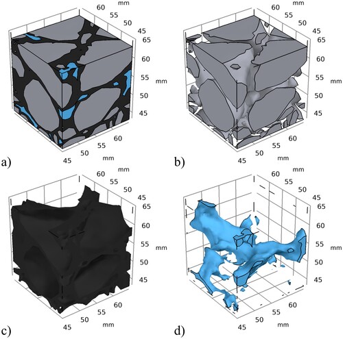
To determine the macroscale damage model parameters, a set of FE simulated tests using the microscale model was utilised. For this purpose, a microscale FE mesh, shown in Figure 1 was used. The mesh was obtained by using X-ray CT scans of a real asphalt mixture sample and resulted in a geometry consisting of 59.3 volume% aggregates ($2\mathrm{m}\mathrm{m}\le \mathrm{d}\le 16\mathrm{m}\mathrm{m}$), 32.1 volume% mastic, and 8.6% air voids.¹ From these simulations, the overall damage evolution of the microstructure was obtained. Thereafter, FE macroscale simulations were performed and the macroscale damage model parameters were calibrated by minimising the difference between the macroscale damage evolution and the microscale damage evolution.

Figure 1. (a) The microstructure, (b) the aggregates, (c) the mastic and (d) the air voids.

The microscale model material parameters used in the simulations are summarised in Table 1. The parameters are either obtained from the literature (de Souza et al. 2004, Kringos et al. 2008a, Kim and Buttlar 2009, Aragão et al. 2011, Yin et al. 2012, Apeagyei et al. 2014, Shakiba et al. 2014, Wang et al. 2014) or assumed to achieve a reasonable behaviour. This is marked in the table by colouring all the values obtained from the literature in blue, while the set values are black. As there is no increase of the damage surface, the values of $K_1$ and $K_2$ are not relevant.

Table 1. Summary of the material properties of the components on the microscale (colour online).

Mastic			Aggregates	Air voids
Diffusive properties
	$\mathrm{D}=1.5\cdot {10}^{-12}$ m^2/s		$\mathrm{D}=2\cdot {10}^{-10}$ m^3/s	$\mathrm{D}=2.8\cdot {10}^{-4}$ m^2/s
Mechanical properties
	$\nu =0.35$		$\nu =0.15$	$\nu =0.31$
	$E_i^L$	${\tau }_i^L$	$E=5\cdot {10}^4$ MPa	$E=8.7\cdot {10}^3$ MPa
1	$4.5\cdot {10}^3$	$1\cdot {10}^{-4}$
2	$1.7\cdot {10}^3$	$1\cdot {10}^{-2}$
3	$2.5\cdot {10}^2$	$1\cdot {10}^0$
4	$2.0\cdot {10}^1$	$1\cdot {10}^2$
∞	$1.6\cdot {10}^2$	–
$C_1=19$, $C_2=150$ K, $T_{ref}^L=293.15$ K
Damage properties
Moisture damage
$p=1.14\cdot {10}^{-6}$ s^-1, r=8
Adhesive mechanical damage
${\sigma }_{I,II0}=3.44$ MPa
$G_{I0}=77$ J/m^2, $G_{II0}=231$ J/m^2
Cohesive mechanical damage
$Y_0^{L,\mathrm{\Psi }}=2\cdot {10}^{10}$ J/m^3, $k=5\cdot {10}^4$ J/m^3
$\omega =0$, n=1

Note: Blue text indicates that the values are obtained from the literature while black text means they are set.

3.1. Moisture damage parameters

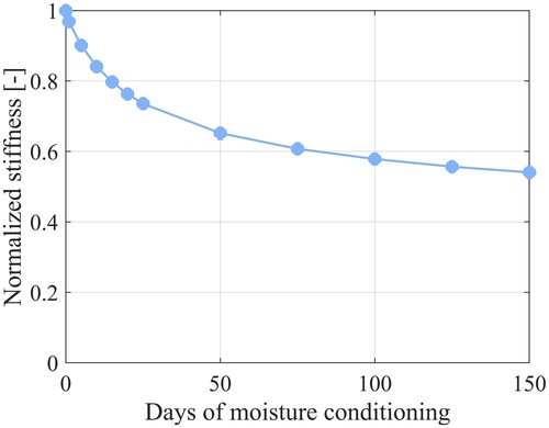
In this section, the parameters P and R which control the moisture damage evolution are determined. The calibration is performed by using a multiscale approach where the results on the microscale are used to determine the macroscale parameters. To do this for the moisture damage parameters, the microstructure depicted in Figure 1 is subjected to moisture, with a normalised concentration of 1, from the top surface for a selected range of times up to 150 days. The resulting adhesive and cohesive moisture damage evolution is shown in Figure 2. This damage causes an overall stiffness degradation of the microstructure which can be evaluated for these selected times by subjecting the microstructure to a compression test, as seen in Figure 3. From the calculated stiffness degradation, the overall effective damage for the microstructure can be calculated by using the relations in Equations (2(2) $\tilde{\mathit{\sigma }}=\frac{\mathit{\sigma }}{1-d},$(2) ) and (3(3) $\psi (\tilde{\mathit{\sigma }},\widetilde{\mathit{ϵ}})=\psi (\mathit{\sigma },\mathit{ϵ}),$(3) ).

Figure 2. Microscale adhesive damage after being subjected to moisture for (a) 10 days, (b) 50 days, and (c) 150 days, and cohesive damage after (d) 10 days, (e) 50 days, and (f) 150 days.

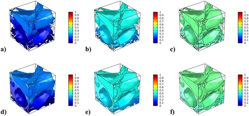
Figure 3. Effective stiffness of the microstructure after being subjected to moisture.

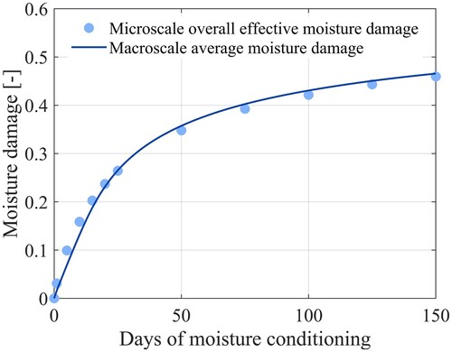
These results are then used to calibrate P and R for the asphalt on the macroscale by comparing the macroscale moisture damage evolution to the one on the microscale. This fitting is performed by utilising the optimisation module in Comsol Multiphysics, which minimises the squared difference between the macroscale and microscale results. A comparison between the fitted macroscale damage evolution and the microscale overall effective damage is shown in Figure 4.

Figure 4. Comparison of the macroscale and microscale predictions of the effective moisture damage evolution.

3.2. Elastic strain energy damage parameters

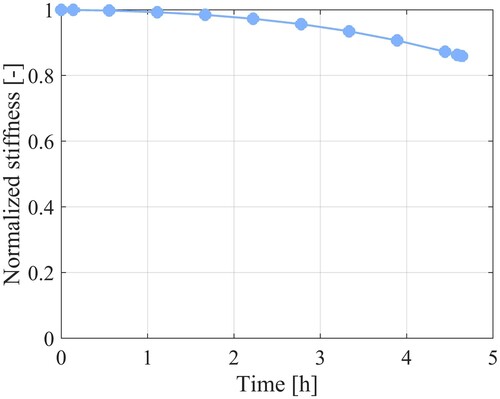
This section regards the calibration of the parameters related to the elastic strain energy damage for the asphalt on the microscale. To do this, a creep test is first performed on the microscale where a stress of 3 MPa is applied on the top of the microstructure at a temperature of $0^{\circ }\mathrm{C}$. It should be noted that this load is not chosen to represent an actual traffic load but to get a feasibly fast damage evolution at the low temperature of the simulated test. The adhesive and cohesive damage evolutions caused by the creep load are shown in Figure 5. The overall stiffness of the microstructure is evaluated at different times during the test, and the resulting degradation of the normalised stiffness is shown in Figure 6.

Figure 5. Microscale adhesive damage after being subjected to a creep load for (a) 1000 s (0.28 h), (b) 10,000 s (2.8 h), and (c) 16,800 s (4.7 h), and cohesive damage after (d) 1000 s (0.28 h), (e) 10,000 s (2.8 h), and (f) 16,800 s (4.7 h).

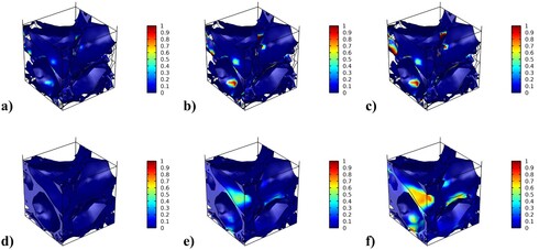
Figure 6. Effective stiffness of the microstructure during the creep test.

For the calibration of the macroscale damage parameters, the reference temperature in the temperature dependency function, $T_0^G$, is set as the creep test temperature $0^{\circ }\mathrm{C}$, i.e. 273.15 K, thus removing the influence of the temperature dependency function, and thereby also the effect of the parameter ${\xi }^G$. Additionally, as there is no size increase of the damage surface on the microscale, the same is assumed for the macroscale by setting the parameter Ω as 0. The material parameters $K_3$ and $K_4$ therefore do not need to be determined. For the case that the material of interest has a damage behaviour where the damage rate decreases after some time such that it ‘hardens’, similar to e.g. plastic hardening, these parameters can be included in the calibration to be able to accurately capture the damage behaviour. 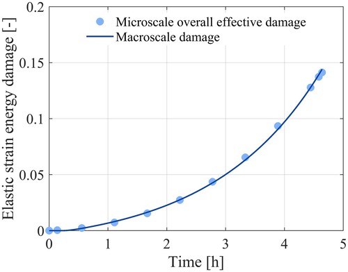The only parameters left to determine is thus the damage initiation threshold $Y_0^{G,E}$ and the damage evolution parameter K. These are determined by applying the same creep load on an asphalt mixture cube on the macroscale and fitting the resulting damage evolution curve to the one obtained from the microscale model simulation. A comparison between the resulting macroscale damage curve and the microscale curves is shown in Figure 7.

Figure 7. Comparison of the macroscale and microscale predictions of the effective elastic strain energy damage evolution.

Since this paper focuses purely on the behaviour of the asphalt mixture in the freezing temperature range, the temperature dependency of the elastic strain energy damage is assumed to be negligible. The material parameter ${\xi }^G$ is therefore not determined in this paper. For the case that a larger temperature range is of interest and ${\xi }^G$ would need to be determined, creep tests at different temperatures on both scales need to be performed. By fixing the already found values of $Y_0^{G,E}$ and K, the temperature dependency could easily be calibrated by fitting the macroscale creep curves to the microscale ones at the different temperatures.

3.3. Freeze-thaw damage parameters

This section regards the calibration of the parameters which control the damage evolution due to freeze-thaw cycles. Only the parameters which affect the original damage evolution, i.e. not the accelerated damage evolution, are calibrated in this paper. The parameters A and B which control the accelerated evolution can in the future be calibrated by using a microstructure with different air void contents and relating these contents to the damage evolution.

The calibration is performed by using a multiscale approach where the microstructure is firstly subjected to 10 consecutive freeze-thaw cycles where each cycle consisted of 6 h freezing from $1^{\circ }\mathrm{C}$ to $-1^{\circ }\mathrm{C}$, 6 h at a constant freezing temperature of $-1^{\circ }\mathrm{C}$, 6 h thawing from $-1^{\circ }\mathrm{C}$ to $1^{\circ }\mathrm{C}$, and finally 6 h at a constant thawing temperature of $1^{\circ }\mathrm{C}$. 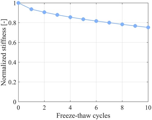Figure 8 shows the resulting evolution of the cohesive damage. Since the adhesive damage caused by the freeze-thaw cycles was minimal, it is not shown in this paper. Thereafter, the degradation of the entire microstructure can be evaluated by performing a simulated compression test on the microstructure to obtain its effective stiffness degradation, shown in Figure 9. The stiffness is evaluated both at an undamaged nominal state before the microstructure was subjected to any freeze-thaw cycles and after each freeze-thaw cycle.

Figure 8. Microscale cohesive damage after being subjected to (a) 2 FTCs, (b) 6 FTCs and (c) 10 FTCs.

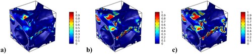
Figure 9. Effective stiffness of the microstructure after being subjected to freeze-thaw cycles.

By recalculating the normalised stiffness degradation to the overall effective damage, the macroscale parameters can be calibrated. In order to only determine the damage evolution parameters without having to account for an accelerated damage effect due to an increased effective air void content, it is assumed that no moisture infiltrates the asphalt mixture during the freeze-thaw cycles such that ${\mathrm{\Theta }}^{eff}$ is 0. The accelerated effect is thus removed. Before the calibration, the values of a and $k_1$ are fixed to ensure the correct amplitude of the damage and q is, for the sake of simplicity, set as 1. Thereafter the remaining parameters, κ, $k_2$ and S are calibrated by minimising the squared difference between the microscale and macroscale results with the help of the optimisation module in Comsol Multiphysics. The resulting damage evolution on the macroscale is compared with the one on the microscale in Figure 10. The result of the identification of all the damage parameters is summarised in Table 2.

Figure 10. Comparison of the macroscale and microscale predictions of the effective FTC damage evolution.

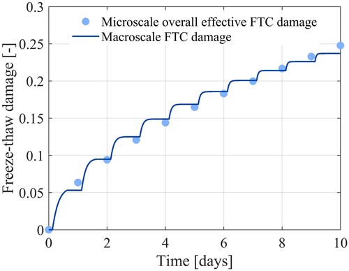
Table 2. Summary of the material properties of the components on the macroscale (colour online).

Diffusive properties
$D=4.8\cdot {10}^{-11}$ m^2/s
Mechanical properties
$\nu =0.15$
	$E_i^G$ [MPa]	${\tau }_i^G$ [s]
1	$3.0\cdot {10}^2$	$2\cdot {10}^{-3}$
2	$6.9\cdot {10}^2$	$2\cdot {10}^{-1}$
3	$2.9\cdot {10}^2$	$2\cdot {10}^1$
4	$6.5\cdot {10}^1$	$2\cdot {10}^3$
∞	$3.2\cdot {10}^2$	–
$C_1=19$, $C_2=150$ K, $T_{ref}^G=293.15$ K
Damage properties
Moisture damage	Strain energy damage	Freeze-thaw damage
$P=2.19\cdot {10}^{-6}$ [1/s]	$K=3.06\cdot {10}^8$ [J/m^3]	$A=37[-]$
$R=9.36[-]$	$N=1[-]$	$a=1.6\cdot {10}^9$ [J/m^3]
	$T_0=273.15$ [K]	$B=2\cdot {10}^7$ [J/m^3]
	$Y_0^{G,E}=1.4\cdot {10}^4$ [J/m^3]	$k_1=4.5\cdot {10}^8$ [J/m^3]
	${\xi }^G=na[-]$	$k_2=1.37[-]$
	$\mathrm{\Omega }=0[-]$	$\kappa =5.98[-]$
		$S=5.25\cdot {10}^{14}$ [J/m^3]
		$q=1[-]$

Note: Blue text indicates that the values are obtained from the literature, red that they are calibrated through the multiscale coupling described in Section 3, and black text means they are set.

4. Case study: effect of different weather conditions on the damage development

In this section, different FE simulation case studies are used to present and highlight the capabilities of the developed model and how it can be used to predict the damage development depending on the surrounding weather conditions. The examples will focus on the novelties of the model presented in this paper: the coupling between moisture damage, freeze-thaw damage and elastic strain energy damage, as well as the inclusion of the accelerated freeze-thaw damage effect. The simulations are performed with the macroscale model on an FE mesh with the dimensions $0.1\times 0.1\times 0.1\mathrm{m}$, representing part of the surface layer of an asphalt mixture pavement. The mesh consisted of $8\times 8\times 8$ elements. The material parameters used in the simulations are summarised in Table 2. The table is colour coded such that blue text means that the values are obtained from the literature (Chen et al. 2017), red that they are calibrated through the multiscale coupling described in Section 3, and black text means they are set.

4.1. Case study 1 – effect of long-term moisture exposure

This case study demonstrates the important model feature of the coupling between moisture damage and freeze-thaw damage. In order to highlight this, two different weather scenarios are considered: one including only freeze-thaw cycles and one combining freeze-thaw cycles and long-term moisture exposure. In the first scenario, it is assumed that the asphalt pavement sample is subjected to freeze-thaw cycles for ten consecutive days. Each freeze-thaw cycle consists of 6 h of freezing from $1^{\circ }\mathrm{C}$ to $-1^{\circ }\mathrm{C}$, 6 h at a constant temperature of $-1^{\circ }\mathrm{C}$, 6 h of thawing back to $1^{\circ }\mathrm{C}$ and then 6 h at a constant temperature of $1^{\circ }\mathrm{C}$. It is assumed that the freeze-thaw cycles are preceded by only a quick rainfall such that the air voids are filled with moisture but the moisture does not infiltrate the asphalt more such that moisture damage is caused. In the second weather scenario, the asphalt layer sample is subjected to a rain fall from the top for 30 days before it is subjected to the same freeze-thaw cycles as in the first scenario. As it is assumed that no moisture infiltrates the material in between the freeze-thaw cycles in these simulations, there is no accelerated effect of the damage development in either of the scenarios.

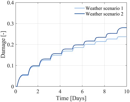
The results from the simulations are shown in Figure 11, in the form of contour plots, and in Figure 12, in the form of the damage evolution on the top and bottom surface of the pavement section. The damage development in the first scenario, shown in Figure 12(a), is the same as the one calibrated in Section 3.3, since the same temperature scenario is used and no moisture or load is applied. The damage development in the second scenario, however, looks different as is seen in Figure 12(b). First, the damage development is different on the bottom surface of the layer than on the top layer, since the moisture infiltrates from the top and thereafter moves downwards which causes a damage gradient, clearly visualised in Figure 11. As seen in Figure 12(b), not enough moisture has yet reached the bottom of the asphalt layer at the end of the assumed rainfall of 30 days to result in any visible damage. The damage development on the bottom surface is thus similar to the one in weather scenario 1. Since it is assumed that the entire pavement section is fully saturated with moisture in the ‘air voids’ such that the freeze-thaw damage is homogenous, there is no difference between the damage development on the top and bottom of the simulated section in the first scenario. On the top surface of the asphalt layer, however, which was directly subjected to the moisture, there is a clear effect of the moisture damage which results in a total damage of around 0.38 at the beginning of the freeze-thaw cycles. In the field this would effectively mean that there is a high risk of ravelling already after 1 freeze-thaw cycle, if moisture has been trapped inside the pavement for a long period of time causing long-term moisture damage. This is a known phenomenon, which has previously been reported in for example Vulcano-Greullet et al. (2010). Being able to account for both the long-term moisture exposure as well as freeze-thaw cycles and their combined effect is therefore important in order to be able to accurately predict the risk of ravelling of a pavement.

Figure 11. Damage development in Weather scenario 1 after (a) 5 days and (b) 10 days, and damage development in Weather scenario 2 after (c) 5 days and (d) 10 days.

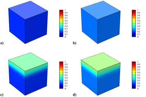
Figure 12. (a) Damage development in Weather scenario 1, (b) damage development in Weather scenario 2 and (c) overall stiffness degradation of the material in the two scenarios.

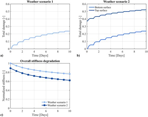
In addition to increasing the risk of ravelling, the combined moisture and freeze-thaw damage also give a larger degrading effect on the material properties than the freeze-thaw damage does on its own. This was investigated by subjecting the sample to a direct compression test to evaluate its stiffness. The result, in the form of a normalised stiffness with the completely undamaged sample as reference, is shown in Figure 12(c). It can be seen that the stiffness degradation in scenario 1 directly corresponds to the damage evolution, due to the homogeneity of the freeze-thaw damage. The degradation of the overall stiffness in scenario 2, however, can be seen to not correspond directly to the damage development on neither the top surface nor the bottom surface. It is instead naturally affected by the damage development in the entire sample and gives a stiffness degradation of around 10% already after the simulated rainfall and around 40% after the freeze-thaw cycles. This can be compared to the stiffness degradation of 24% after only the freeze-thaw cycles in the first weather scenario. Ultimately this can have large consequences on the behaviour of the pavement and can affect for example the rutting.

These results demonstrate the importance of understanding the sensitivity of asphalt mixtures to long-term moisture exposure, freeze-thaw cycles and their coupled effect. Not accounting for the two damage sources and their coupling in the prediction could thus lead to a significant underestimation of the timing and extent of the damage that will occur. Ultimately, this can cause erroneous decisions regarding the material design which consequently can lead to disastrous results such as premature and rapid failure.

4.2. Case study 2 – effect of accelerated freeze-thaw damage due to an increased air void content

In the second case study, the model feature which accounts for the effect of the accelerated damage due to an increased effective air void volume is highlighted. Two weather scenarios are used to showcase this. The first scenario equals the first scenario in the previous case study with 10 consecutive freeze-thaw cycles and a quick preceding rainfall but no moisture damage or acceleration of damage as no moisture is assumed to infiltrate the pavement between the freeze-thaw cycles. In the second scenario, the asphalt pavement sample is subjected to the same quick rainfall and 10 freeze-thaw cycles but with the addition that it is also subjected to quick rainfalls, or melting snow, between every freeze-thaw cycle which is assumed to fill the enlarged pore space such that the damage is accelerated but does not cause any moisture damage due to the short time period between the cycles.

The evolutions of freeze-thaw damage for both scenarios are shown in Figure 13. It can be seen that there is a clear difference in the resulting damage between the two scenarios. Due to the formulation of the accelerating part of the damage, the difference between the two damage evolutions is almost negligible after the first freeze-thaw cycle. As the damage is so low after only one freeze-thaw cycle, the hypothesised increase of air void volume and the related accelerated effect is thereby also low. After the first freeze-thaw cycle, the effect is becoming more visible and as the damage increases, so does the accelerating effect. The difference in damage increase rate between the scenarios is thus the largest after the 10th freeze-thaw where the damage increase in the first scenario is the smallest but in the second scenario is the largest. This can thus lead to a rapid increase of damage which ultimately could cause an explosion of damage. It can thus be concluded that this effect is important to consider when predicting the damage as failure to do so can lead to an underestimation of the predicted damage which can cause erroneous decisions regarding material design. It is thus important to further investigate this effect experimentally and to account for it when making damage predictions.

Figure 13. Damage development during the two scenarios.

4.3. Case study 3 – effect of combined mechanical and environmental loading

The two previous case studies only accounted for the environmental damaging effects and not any external mechanical loading, such as caused by traffic. In this case study, the effect of mechanical loading and, specifically, its combined effect with different weather scenarios is studied. This is performed by again considering two different weather scenarios: one which does not account for moisture and freeze-thaw cycles and one which does. Both scenarios include a constant pressure of 2 MPa on top of the pavement section. It should be noted that the load is not representative of an actual traffic load but chosen to clearly show the effect of combining the damage sources under the considered material properties and loading times. Additionally, it should also be noted that the applied load only represents the weight of the traffic and does not include the effect of the pumping action of any moisture inside the voids which the traffic may also cause in reality.

In the first scenario, no moisture and freeze-thaw damage is included by assuming completely dry conditions and a constant temperature of $0^{\circ }\mathrm{C}$. This scenario thus considers the effect of only the applied pressure on the behaviour of the asphalt mixture. The second scenario assumes a combination of rain and freeze-thaw cycles, thus including both moisture and freeze-thaw damage in addition to any strain energy based damage caused by the mechanical load. In the second scenario, each freeze-thaw cycle consists of 6 h of freezing from $1^{\circ }\mathrm{C}$ to $-1^{\circ }\mathrm{C}$, 30 h at a constant temperature of $-1^{\circ }\mathrm{C}$, 6 h of thawing from $-1^{\circ }\mathrm{C}$ to $1^{\circ }\mathrm{C}$, and finally 30 h at a constant temperature of $1^{\circ }\mathrm{C}$. During the periods with a temperature above $0^{\circ }\mathrm{C}$, it is assumed that the asphalt pavement section is subjected to moisture, either through rain or through melting snow such that there is an acceleration of the freeze-thaw damage development.

The damage evolution and the axial strain of the pavement section caused by the load are shown in Figure 14 for both scenarios. In Figure 14(a), it can be seen that no damage is caused by only applying a mechanical load. This thus means that the strain, shown in Figure 14(b), only goes through the primary and secondary stages of creep but does not reach the tertiary stage. There is thus no failure of the pavement.

Figure 14. (a) The damage curves for both scenarios and (b) the axial strain of the pavement for both scenarios.

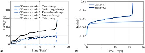
As the second weather scenario also includes moisture and freeze-thaw conditioning, there is a continuous increase of damage throughout the simulated period. It should be noted that the moisture damage is constant during the freezing periods as it is assumed that all moisture inside the pavement at that time is ice and therefore only deteriorates the material in the form of freeze-thaw damage. The moisture and freeze-thaw damage clearly affects the strain of the pavement and results in a larger deformation already from the beginning of the period. This existing damage affects the strain and thereby also the elastic strain energy release rate for the strain energy based damage, $Y^{G,E}$, according to Equation (83(83) $Y^{G,E}=-\frac{\mathrm{\partial }{\psi }^G}{\mathrm{\partial }{d}^{G,E}}=\frac{{\mathit{\sigma }}^{G,\mathrm{\infty }}}{(1-d^{G,E})}:{\mathit{ϵ}}_n^G+\sum _{n=1}^N\frac{{\mathit{\sigma }}_n^{G,v}}{(1-d^{G,E})}:({\mathit{ϵ}}_n^G-{\mathit{ϵ}}_n^{G,v}),$(83) ). Consequently, it can be seen that this causes elastic strain energy based damage to initiate and evolve after around 15 days of moisture and freeze-thaw exposure and mechanical loading. The rapid evolution of the strain energy based damage, and thus also the total damage, clearly affects the strain which is seen to reach the tertiary stage. This naturally ultimately leads to loss of the structural integrity and failure of the pavement.

These results clearly show the importance of coupling moisture, freeze-thaw and elastic strain energy damage. By neglecting the effect of long-term moisture and freeze-thaw cycle exposure, the damage prediction can be severely underestimated. Decisions made based on the wrong information or currently inaccurate data can thus lead to catastrophic consequences.

5. Summary and conclusion

The aim of this paper was to develop a multiscale model which is able of predicting the damage development and can also assist towards understanding and characterising the damage evolution and how the different material components affect it. The developed model therefore consists of two scales: a local microscale including mastic, aggregates and air voids, and a global macroscale of the homogenised asphalt mixture. To ensure that the models on both scales can be applied for a range of different conditions, the equations were based on the thermodynamical restrictions.

The microscale model features diffusion of moisture through the mixture, the expansion and contraction of the air voids as the water inside them freezes and thaws, and the coupled damage from both these mechanisms in the form of both cohesive damage inside the mastic and adhesive damage in the mastic-aggregate interface. The macroscale model includes the coupled damage evolution due to the combination of moisture, freeze-thaw cycles and external mechanical loads which affect the elastic strain energy (i.e. resulting from traffic loading). To account for the damaging effect of freeze-thaw cycles without explicitly modelling the expansion and contraction, a separate damage variable for the freeze-thaw damage is included. This work also hypothesises an accelerated effect of the freeze thaw damage, which is caused if more moisture infiltrates the damaged asphalt pavement between freeze-thaw cycles. This was modelled by letting the development depend on the existing damage, thus introducing a history dependency.

The coupling between the two scales was done by letting the damage behaviour of the macroscale depend on the effective damage behaviour of the microscale. This was illustrated by calibrating the macroscale damage parameters with the help of microscale simulations.

The novelty of this model lies in the multiscale coupling of the freeze-thaw damage, the inclusion of the accelerated damage effect, as well as the coupled effect between moisture, freeze-thaw and elastic strain energy damage. This is demonstrated by using the model for predicting the damage development caused by different weather scenarios. It is shown that the model is capable of the risk of ravelling as well as the potential rapid increase of damage which can occur when a pavement is subjected to a combination of moisture, freeze-thaw cycles and traffic. Additionally, the paper demonstrated the importance of investigating the accelerated effect on the freeze-thaw damage evolution caused by infiltration of moisture into a damaged pavement. Underestimating any of these effects when designing an asphalt pavement can thus cause catastrophic and unexpected failures. Since the model is based on a thermodynamical framework, it can be easily extended in the future to include more mechanisms and behaviours, such as pumping action of water in the air voids, plasticity and healing. For future work, it is recommended that the multiscale model is extended to a two-way coupled model where the microstructure is updated. This would enable an even better analysis and prediction of the damage evolution as it could consider the microstructural changes over time.

Disclosure statement

No potential conflict of interest was reported by the author(s).

Additional information

Funding

The authors gratefully acknowledge the support of the Swedish Transport Administration within the BVFF program and the KTH Road2Science Center.

Notes on contributors

Lisa Lövqvist

Lisa Lövqvist has a PhD from KTH Royal Institute of Technology. Her research is on freeze-thaw damage in asphalt pavements, where she focuses on computational modelling of the emergence and evolution of damage.

Romain Balieu

Romain Balieu is Researcher in Highway Engineering at KTH. His research focuses on computational modelling and assessment of sustainable transportation infrastructure.

Nicole Kringos

Nicole Kringos is Professor in Highway Engineering at KTH and the Scientific Director of the KTH Road2Science Competence Center. Her research group focuses on developing computational tools that support the design, building and maintenance of sustainable transportation infrastructure.

Notes

1 Note that the used microstructure is too small in relation to the largest aggregate to be considered a proper RVE. As this work only aims to present the developed model, a smaller microstructure was used for simulation reasons. For works that aim to validate the model or perform a proper analysis, it is vital that a proper RVE is used.

References

- Aigner, E., Lackner, R., and Pichler, C., 2009. Multiscale prediction of viscoelastic properties of asphalt concrete. Journal of Materials in Civil Engineering, 21 (12), 771–780.
- Allen, D.H., 2001. Homogenization principles and their application to continuum damage mechanics. Composites Science and Technology, 61 (15), 2223–2230. Available from: https://www.sciencedirect.com/science/article/pii/S0266353801001166.
- Allen, D.H., et al., 2017a. Multi-scale computational model for design of flexible pavement–part I: expanding multi-scaling. International Journal of Pavement Engineering, 18 (4), 309–320. Available from: http://dx.doi.org/10.1080/10298436.2015.1065999.
- Allen, D.H., et al., 2017b. Multi-scale computational model for design of flexible pavement–part II: contracting multi-scaling. International Journal of Pavement Engineering, 18 (4), 321–334. Available from: http://dx.doi.org/10.1080/10298436.2015.1066000.
- Allen, D.H., et al., 2017c. Multi-scale computational model for design of flexible pavement–part III: two-way coupled multi-scaling. International Journal of Pavement Engineering, 18 (4), 335–348. Available from: http://dx.doi.org/10.1080/10298436.2015.1066001.
- Apeagyei, A.K., Grenfell, J.R.A., and Airey, G.D., 2014. Evaluation of moisture sorption and diffusion characteristics of asphalt mastics using manual and automated gravimetric sorption techniques. Journal of Materials in Civil Engineering, 26 (8), 04014045.
- Aragão, F.T.S., et al., 2011. Micromechanical model for heterogeneous asphalt concrete mixtures subjected to fracture failure. Journal of Materials in Civil Engineering, 23 (1), 30–38.
- Balieu, R. and Kringos, N., 2015. A new thermodynamical framework for finite strain multiplicative elastoplasticity coupled to anisotropic damage. International Journal of Plasticity, 70, 126–150. Available from: http://dx.doi.org/10.1016/j.ijplas.2015.03.006.
- Chen, F., Balieu, R., and Kringos, N., 2017. Thermodynamics-based finite strain viscoelastic-viscoplastic model coupled with damage for asphalt material. International Journal of Solids and Structures, 129, 61–73. Available from: https://doi.org/10.1016/j.ijsolstr.2017.09.014.
- de Souza, F.V., et al., 2004. Model for predicting damage evolution in heterogeneous viscoelastic asphaltic mixtures. Transportation Research Record, 1891, 131–139.
- Feng, D., et al., 2010. Impact of salt and freeze-thaw cycles on performance of asphalt mixtures in coastal frozen region of China. Cold Regions Science and Technology, 62 (1), 34–41. Available from: http://dx.doi.org/10.1016/j.coldregions.2010.02.002.
- Füssl, J. and Lackner, R., 2011. Multiscale fatigue model for bituminous mixtures. International Journal of Fatigue, 33 (11), 1435–1450.
- Garcia Cucalon, L., et al., 2016. A multiscale model for predicting the viscoelastic properties of asphalt concrete. Mechanics of Time-Dependent Materials, 20 (3), 325–342. Available from: http://dx.doi.org/10.1007/s11043-016-9303-2.
- Kachanov, L., 1958. Time of the rupture process under creep conditions. Izvestiia Akademii Nauk SSSR, 8, 26–31. (In Russian).
- Kim, H. and Buttlar, W.G., 2009. Discrete fracture modeling of asphalt concrete. International Journal of Solids and Structures, 46 (13), 2593–2604. Available from: http://dx.doi.org/10.1016/j.ijsolstr.2009.02.006.
- Kringos, N., et al., 2008b. Modelling of combined physical-mechanical moisture-induced damage in asphaltic mixes, Part 1: Governing processes and formulations. International Journal of Pavement Engineering, 9 (2), 115–128.
- Kringos, N., et al., 2008c. Modelling of combined physical-mechanical moisture-induced damage in asphaltic mixes Part 2: Moisture susceptibility parameters. International Journal of Pavement Engineering, 9 (2), 129–151.
- Kringos, N. and Liu, X., 2004. Multi-phase material model for freezing damage in open graded asphaltic mixes. In: Proceedings of the 2004 international conference on computational & experimental engineering & sciences, Madeira, Portugal.
- Kringos, N., Scarpas, A., and de Bondt, A., 2008a. Determination of moisture susceptibility of mastic-stone bond strength and comparison to thermodynamical properties. In: Journal of the association of asphalt paving technologists, Vol. 77, Philadelphia, PA, USA: Association of Asphalt Paving Technologists (AAPT).
- Lövqvist, L., Balieu, R., and Kringos, N., 2020a. A step towards a multiscale model of frost damage in asphalt mixtures. In: A. Kumar, A. Papagiannakis, A. Bhasin and D. Little, eds. Advances in materials and pavement performance prediction II. CRC Press, 295–298.
- Lövqvist, L., Balieu, R., and Kringos, N., 2020b. A thermodynamics-based model for freeze-thaw damage in asphalt mixtures. International Journal of Solids and Structures, 203, 264–275.
- Lövqvist, L., Balieu, R., and Kringos, N., 2021. A micromechanical model of freeze-thaw damage in asphalt mixtures. International Journal of Pavement Engineering, 22 (8), 1017–1029. Available from: https://doi.org/10.1080/10298436.2019.1656808.
- Luo, Y., et al., 2017. The deterioration and performance improvement of long-term mechanical properties of warm-mix asphalt mixtures under special environmental conditions. Construction and Building Materials, 135, 622–631. Available from: http://dx.doi.org/10.1016/j.conbuildmat.2016.12.167.
- Lutif, J.E., et al., 2010. Multiscale modeling to predict mechanical behavior of asphalt mixtures. Transportation Research Record, 2181, 28–35.
- Onifade, I., Birgisson, B., and Balieu, R., 2015. Energy-based damage and fracture framework for viscoelastic asphalt concrete. Engineering Fracture Mechanics, 145, 67–85. Available from: http://dx.doi.org/10.1016/j.engfracmech.2015.07.003.
- Pan, P., et al., 2017. Effect of freezing-thawing and ageing on thermal characteristics and mechanical properties of conductive asphalt concrete. Construction and Building Materials, 140, 239–247. Available from: http://dx.doi.org/10.1016/j.conbuildmat.2017.02.135.
- Rabotnov, Y., 1969. Creep problems in structural members. Amsterdam: North-Holland Pub. Co.
- Shakiba, M., et al., 2014. Microstructural modeling of asphalt concrete using a coupled moisture-mechanical constitutive relationship. International Journal of Solids and Structures, 51 (25-26), 4260–4279. Available from: http://dx.doi.org/10.1016/j.ijsolstr.2014.08.012.
- Shakiba, M., Darabi, M.K., and Abu Al-Rub, R.K., 2016. A thermodynamic framework for constitutive modeling of coupled moisture-mechanical induced damage in partially saturated viscous porous media. Mechanics of Materials, 96, 53–75.
- Si, W., et al., 2014. Reliability-based assessment of deteriorating performance to asphalt pavement under freeze-thaw cycles in cold regions. Construction and Building Materials, 68, 572–579. Available from: http://dx.doi.org/10.1016/j.conbuildmat.2014.07.004.
- Souza, F.V., and Allen, D.H., 2010. Multiscale modeling of impact on heterogeneous viscoelastic solids containing evolving microcracks. International Journal for Numerical Methods in Engineering, 82, 464–504.
- Souza, F.V., Allen, D.H., and Kim, Y.R., 2008. Multiscale model for predicting damage evolution in composites due to impact loading. Composites Science and Technology, 68 (13), 2624–2634.
- Sun, Y., et al., 2019. Analysis of load-induced top-down cracking initiation in asphalt pavements using a two-dimensional microstructure-based multiscale finite element method. Engineering Fracture Mechanics, 216 (May), 106497. Available from: https://doi.org/10.1016/j.engfracmech.2019.106497.
- Teixeira, J.E.S.L., et al., 2014. Multiscale model for asphalt mixtures subjected to cracking and viscoelastic deformation. Transportation Research Record, 2447, 136–145.
- Varveri, A., et al., 2014. A constitutive model for simulation of water to ice phase change in asphalt mixtures. In: Asphalt pavements – proceedings of the international conference on asphalt pavements, ISAP 2014, 1 (June). 531–539.
- Varveri, A., Zhu, J., and Kringos, N., 2015. Moisture damage in asphaltic mixtures. In: S.-C. Huang and H. Di Benedetto, eds. Advances in asphalt materials: road and pavement construction. Cambridge: Woodhead Publishing, 303–344.
- Vulcano-Greullet, N., et al., 2010. Stripping phenomenon in thick pavement top layers. In: Proceedings of the 11th international conference on asphalt pavements. 552–561.
- Wang, H., Wang, J., and Chen, J., 2014. Micromechanical analysis of asphalt mixture fracture with adhesive and cohesive failure. Engineering Fracture Mechanics, 132, 104–119. Available from: http://dx.doi.org/10.1016/j.engfracmech.2014.10.029.
- Wollny, I., et al., 2020. Coupling of microstructural and macrostructural computational approaches for asphalt pavements under rolling tire load. Computer-Aided Civil and Infrastructure Engineering, 35 (11), 1178–1193.
- Xu, H., Guo, W., and Tan, Y., 2015. Internal structure evolution of asphalt mixtures during freeze-thaw cycles. Materials and Design, 86, 436–446. Available from: http://dx.doi.org/10.1016/j.matdes.2015.07.073.
- Yi, J., et al., 2014. Viscoelastic-plastic damage model for porous asphalt mixtures: Application to uniaxial compression and freeze-thaw damage. Mechanics of Materials, 70, 67–75. Available from: http://dx.doi.org/10.1016/j.mechmat.2013.12.002.
- Yin, A., et al., 2012. Tensile fracture simulation of random heterogeneous asphalt mixture with cohesive crack model. Engineering Fracture Mechanics, 92, 40–55. Available from: http://dx.doi.org/10.1016/j.engfracmech.2012.05.016.
- Zhang, Z., et al., 2021. Damage evolution of asphalt mixture under freeze-thaw cyclic loading from a mechanical perspective. International Journal of Fatigue, 142 (June 2020), 1–9.