Evaluation of the structural response of two in-service thin flexible pavements under heavy vehicle loading during different seasons by built-in sensors

ABSTRACT

Long Heavy Vehicles (LHV) are considered more efficient and environmentally friendly transportation of goods compared to conventional trucks. Thus, the maximum allowable gross vehicle weight (GVW) in Sweden was increased on part of the road network from 64 to 74 tons in 2018 by increasing the vehicles’ length and the number of axle groups per vehicle but not the axle load limits. This change in loading conditions is expected to lead to changes in the structural response and degradation rate of thin pavements on the low-volume road network. To improve our understanding of thin pavements behaviour exposed to multiple axle loadings two thin pavement structures located in the north of Sweden were instrumented with road response and climate sensors. Four measurement campaigns were carried out within one year by in-situ stress and strain measurements from the built-in sensors as LHV passes over at normal speed. The recorded response was compared with numerical calculations based on multilayer elastic theory (MLET). Values of stresses and strains showed a generally good agreement with high values of coefficient of determination R² during different seasons when the asphalt stiffness values were adjusted based on temperature and granular layer stiffness values based on moisture.

KEYWORDS:

• Thin flexible pavement
• built-in sensors
• in-situ response measurement
• long heavy vehicle
• numerical modelling
• seasonal variation

Introduction

In recent years, Longer Heavier Vehicles (LHVs) have become increasingly more popular. LHVs have a higher load-carrying capacity compared to conventional heavy-duty vehicles which can be achieved by increasing the number of axles, length of the vehicles, axle load, and total vehicle weight. Multiple studies have reported that the use of LHVs leads to improvements in transportation cost efficiency (Ortega 2014; Sanchez Rodrigues 2015) and improved environmental performance (Knight 2008; Christidis and Leduc 2009). Most of the research on the impact of LHVs within the transport sector focuses on the vehicles themselves and not on the potential increase in pavement deterioration (Pålsson 2017). The inclusion of the impact of LHVs on pavement construction and maintenance-related costs could improve the accuracy of economic analyses related to LHVs.

The maximum allowable gross vehicle weight (GVW) in Sweden has increased from 60 tons in 1996, to 64 tons in 2015 by the Swedish Transport Administration (Erlingsson et al. 2018). On a limited number of roads, a higher loading of 74 tons is allowed since 2018 as well, an increase which is planned to be implemented on the entire road network in the future (Natanaelsson and Eriksson 2020). A large number of roads in the national network are low volume roads which typically consist of a thin asphalt layer or layers placed over one or more granular layers on top of a compacted subgrade. These roads play an important role in the Swedish economy in particular for the mining and timber industries.

The environmental variables such as temperature and moisture, that surround pavement structures affect considerably their structural behaviour (Doré and Zubeck 2009). It is therefore important to account for the seasonal variation of the environmental variables when analysing the performance of pavements, in particular in areas with large seasonal variations. The temperature and moisture distribution in the cross-section is largely influenced by the boundary conditions of the system. Thus, larger variations occur in the upper part of the structure due to the proximity to the surface boundary. The temperature variations affect the stiffness of the asphalt layers. Frost penetrating into the structure makes the unbound layers stiff and moisture lubricates the granular layers and softens them, particularly during spring thaw (Simonsen and Isacsson 1999; Salour and Erlingsson 2013a; Salour 2015; Erlingsson et al. 2017).

A new Mechanistic-Empirical (M-E) pavement design and performance prediction tool is currently under development in Sweden. It is essential that the response analysis part of the tool can predict the actual induced response in the pavement structure due to the heavy loadings under the prevailing ambient climate conditions. It is therefore important that the M-E scheme considers the shift in vehicle types and the various axle configurations of the vehicles with higher GVW. Several methods are available for modelling the induced response of pavement structures, among them the multilayer elastic theory (MLET) and the finite element method (FEM). FEM is able to model more complex loading conditions, geometries and can incorporate more advanced material models. MLET requires several background assumptions such as isotropic and homogenous layers extending infinitely in the horizontal direction and the applied loading being circular with constant pressure (Burmister 1945; Huang 2004; Erlingsson and Ahmed 2013). However, due to faster computation times, MLET has become the common option of choice in pavement design (ARA Inc. 2004; Loulizi et al. 2006). It has further been shown that the differences in calculated pavement response values between MLET and FEM are negligible in many cases (Saevarsdottir and Erlingsson 2015; Fladvad and Erlingsson 2022). The validation of the pavement response models requires field testing (Ahmed and Erlingsson 2013; Pereira and Pais 2017; Gkyrtis et al. 2021) through instrumented road sections in which sensors are embedded within the pavement structure to measure the actual response (Gusfeldt and Dempwolff 1967; Hicks and Finn 1970; Terrell and Krukar 1970; Al-Qadi et al. 2004; Blanc et al. 2019; Duong et al. 2019).

In this paper, the response signals obtained from two instrumented thin flexible pavements subjected to loading by three different LHVs have been evaluated at four different times of measurements over 12 months. The primary aim is to investigate the effects of seasonal variations of the environmental variables on the response of pavement structures due to LHV. Furthermore, the response signals have been compared against MLET-calculated values. The layer stiffness values were obtained by falling weight deflectometer (FWD) backcalculation (Irwin 2002) and simultaneously adjusted for temperature and moisture variations to reflect the actual field conditions. The measurement-calculation comparison of the instrumented test sections was used to validate the numerically predicted structural response to be used in the new M-E calculation scheme.

Description of the test sites and instrumentation procedure

For this research presented here, two road sections were selected to be instrumented during autumn 2017 (Saliko and Erlingsson 2021). The sections are located in the northern part of Sweden along the roads Lv373 (section 58,980 m) and Lv515 (section 1360 m) notations by which they are referred to in this paper. The sections are located approximately 10 km apart from each other. The coordinates for the location of Lv373 are N65.33741, E20.4675 and for Lv515 N65.31813, E20.29687.

To monitor the mechanical response of the structures, asphalt strain gauges (ASGs), soil pressure cells (SPCs), and strain measuring units (ϵMU coils) were used. Two trenches were made in each of the structures in order to obtain two set-ups of instrumentation which reduces the risk of loss of data due to possible malfunctions. The ASGs were installed underneath the asphalt concrete (AC) layer in two directions, along the wheel path and perpendicular to it. This was done to measure the longitudinal and transversal strains in the bottom of the asphalt concrete layer when loading was applied on the surface. The ϵMU coils and SPCs were installed in the granular layers of the structure to measure the induced vertical strain and stress respectively. More details on the sensors used in this study can be found in Saevarsdottir et al. (2016).

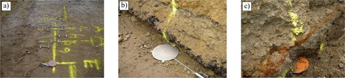
The installation procedure began with the removal of the top AC layer along 20 m in one of the two lanes. Afterwards, two trenches each of them 1.2 m wide were excavated with a distance of 4 m away from each other. The storage of the excavated material was done separately for each layer to avoid mixing of material from different layers. All existing layer thicknesses were determined during the excavation process. After the excavation was completed, the sensors were installed inside the pavement structure. The excavated material was placed back and compacted layer-by-layer. Finally, a new layer of AC (ABT16) was repaved. The procedure of the sensor installation is illustrated in Figure 1. Pictures taken during the installation procedure are shown in Figure 2.

Figure 1. Illustration of the pavement instrumentation procedure (a) excavation procedure in plan-view, (b) excavation procedure in cross-section-view, (c) installation positions for the sensors, and (d) completed installation.

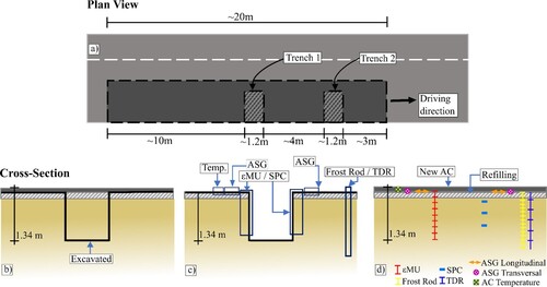
Figure 2. Pictures taken during the installation of the sensors used for the instrumentation procedure (a) ASGs – Asphalt Strain Gauges, (b) SPC – Soil Pressure Cell, and (c) ϵMU coil – Strain Measuring Unit coil.

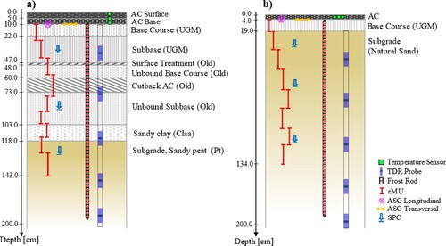
The layer types and thicknesses of the cross-sections of the two pavement structures are illustrated in Figure 3. Both structures are old pavement structures and have had a maintenance history over the years. In the case of Lv373, the original cross-section consisting of cutback AC placed on top of a subbase and a sandy clay layer has been overlaid two times. The first time the structure was overlaid by an unbound granular material (UGM) base course, and a thin surface treatment. Later a new unbound subbase and base course, and a 10 cm AC layer were added. Lv515 is a simpler structure consisting of a thin 4 cm AC layer and a 15 cm unbound base course placed above a natural sandy subgrade.

Figure 3. The layer and sensor configurations for the (a) Lv373 cross-section, and (b) Lv515 cross-section.

The installation of the sensors was performed in a bottom-to-top manner. First, the ϵMU coils were installed in one of the walls of a trench while SPCs were installed in the adjacent wall. After the ϵMU coils and SPCs were placed at a certain depth, the stored material from that layer was placed back and compacted. This was done for all the granular layers. Once all the UGM layers were placed back and compacted, ASGs were installed. The ASGs were not installed on top of the material located in the trench but on top of the base course outside of the trench. This was done to obtain a response that resembles more closely the existing conditions as the material in the trench was disturbed by the excavation. A new layer of AC (ABT16) was thereafter repaved on top of the ASG sensors.

Monitoring the climate seasonal variation

The seasonal variation of the environmental variables was monitored using thermocouples, time-domain reflectometer (TDR) probes, and frost rods. The thermocouples were used to monitor the temperature variation within the AC layer. For Lv373, the thermocouples were installed at 2.5, 5, and 7.5 cm depths. In the case of Lv515, the thermocouples were installed only at 2 cm depth due to the structure’s AC layer thickness limitation. The recording interval for the thermocouples was set to one hour. To monitor the cross-sectional moisture variation, TDR probes were installed in the UGM of the structures. The TDR probes were placed on a 200 cm rod at 5 different depths ranging from 36 cm to 196 cm with 40 cm spacing intervals. The volumetric moisture content values were logged every 20 min. The recorded temperature and volumetric moisture content values for both test sites are shown in Figures 4 and 5.

Figure 4. Recorded values at Lv373 for (a) the daily average AC temperature and (b) the moisture content variation of the unbound granular layers.

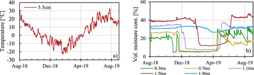
Figure 5. Recorded values at Lv515 for (a) the daily average AC temperature and (b) the moisture content variation of the unbound granular layers.

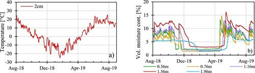
For both structures, the temperature of the asphalt layer and the moisture content in the granular layers have been monitored for a whole year from 1 August 2018 to 31 August 2019. The TDR probes recorded a low moisture content during the winter period followed by a sudden increase during the spring thaw and a gradual decrease during the following recovery period. Peaks in the moisture content levels are recorded during rainy events in the summer and autumn seasons. Since these structures are located in the north of Sweden, the spring thaw period starts in late April and is over in the middle of June.

To monitor the temperature distribution and frost depth in the cross-section of the structures, frost rods were used. The frost rods were made of 41 temperature sensors placed every 5 cm on a 200 cm long bar. The logging was performed at 30-minute intervals. The frost penetration was obtained either directly from a temperature sensor recording 0°C or by linear interpolation between two consecutive sensors where one shows positive and the other negative temperature values to obtain the 0°C isotherm. The recorded temperature distribution and interpolated frost depth for the period 1 October 2018 until 22 June 2019 are presented in Figures 6 and 7.

Figure 6. Cross-sectional temperature variation and frost depth corresponding to the 0°C isotherm for Lv373 from 01 October 2018 to 30 June 2019. The dotted line represents the two dates when response measurements were made.

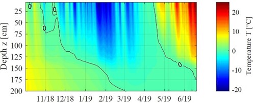
Figure 7. Cross-sectional temperature variation and frost depth corresponding to the 0°C isotherm for Lv515 from 01 October 2018 to 30 June 2019. The dotted line represents the two dates when response measurements were made.

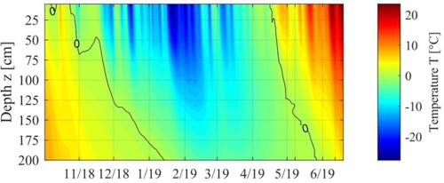
A limitation that applies to the data is the maximum depth of 200 cm due to the length of the frost rod. Nevertheless, it was possible to obtain the beginning of the freezing period, the approximate rate of frost penetration, the beginning of the thawing period, and the approximate rate of thawing.

Backcalculation of the structural response from FWD

Four different testing campaigns over one year have been performed. The dates when the tests were carried out were 29–30 August 2018, 8–9 May 2019, 12–13 June 2019, and 21–22 August 2019. The dates were selected to capture the seasonal variation of the structural behaviour of the test sections with the main focus on the spring thaw period. Each testing campaign included falling weight deflectometer (FWD) measurements and sensor response registrations under controlled application of passing LHV vehicles.

The FWD measurements were performed to later backcalculate the stiffness values of the layers. Three different load levels of 30kN, 50kN, and 65kN were applied. The loading was applied directly on top of the sensors. Afterwards, the 50kN load level was used as a reference for the comparison between the measured FWD deflection bowls and the calculated bowls using the MLET-based software ERAPave (Erlingsson and Ahmed 2013). The algorithm used for the backcalculation procedure is illustrated in Figure 8.

Figure 8. Flowchart illustrating the backcalculation procedure used in the study.

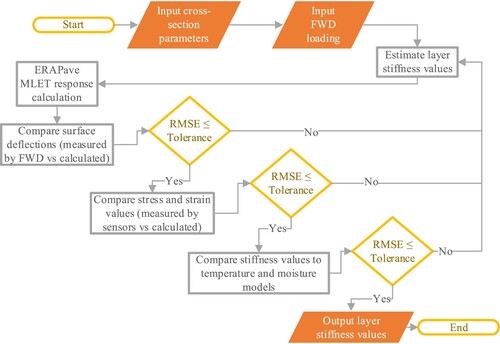
For the backcalculation procedure, both the surface deflection bowl obtained through the deflection sensors of the FWD equipment and the response of the instrumented sensors at the time when the loading was applied were used. The sensors’ response was checked by comparing the longitudinal and transversal strain recorded by ASGs to the calculated values at the bottom of the AC layer, recorded vertical stresses by SPCs, and vertical strains by ϵMU coils to the MLET-calculated values at their corresponding depths. The measurements were divided into two groups. Measurements performed outside the trench corresponding to the ASG sensors and measurements performed inside the trench corresponding to the ϵMU coils and SPCs. The reason for this choice was to take into consideration the disturbance in the excavated and recompacted material inside the trenches. Even though the material inside the trenches was inserted back and compacted thoroughly layer by layer it was not possible to achieve the same compaction level as in the undisturbed material. This is reflected also in the FWD deflection bowls from 50 kN loading as shown in Figure 9.

Figure 9. Deflection bowls under 50kN FWD loading compared to MLET calculations for the campaign (a) August 2018, (b) May 2019, (c) June 2019, and (d) August 2019.

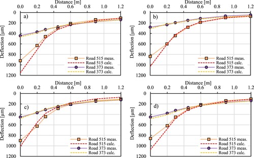
As illustrated in Figure 9, the graphical comparisons between the measured and MLET-calculated deflection bowls show a generally good agreement. An exception to this is the backcalculation for road 515 during the August 2019 campaign illustrated in Figure 9(d) in which a lower quality of fit can be noticed. Backcalculated and measured deflection bowls from FWD loading with 30 and 65 kN exhibited a similar quality of fit and therefore it was decided to initially perform a linear MLET simulation to determine whether it would be possible to capture the general response behaviour of the two pavement structures.

In the process of backcalculating the layer stiffness values, the influence of temperature on the AC layers and the influence of moisture in the UGM was considered.

In this study, the stiffness of the AC layer was adjusted according to (Erlingsson 2012) (1) $E_T=E_{T,ref}\cdot e^{-b(T-T_{ref})}$(1) where E_T is the predicted asphalt stiffness, T_ref is the reference temperature (10°C), E_T,ref is the asphalt stiffness 6500 MPa at the reference temperature, and b is a regression constant of 0.065.

For Lv373, the AC surface and AC base were combined into a single layer as their individual thicknesses were only a small part of the total thickness of the cross-section. The temperature value recorded at the time of FWD measurements from the thermocouple at 5.5 cm depth in the middle of the asphalt layer was used. For Lv515, the value at a depth of 2.0 cm was used.

The variation of the stiffness values of UGM layers has been adjusted using the MEPDG M_R-moisture model (Leong and Rahardjo 1997; ARA Inc. 2004; Andrei et al. 2009) expressed as a function of the degree of saturation (2) $\log {\displaystyle \frac{M_R}{M_{R,opt}}=a+{\displaystyle \frac{b-a}{1+\exp (\beta +k_s(S-S_{opt}))}}}$(2) where M_R is the predicted resilient modulus, M_R,opt is the optimal reference modulus, S is the degree of saturation, S_opt is the optimal degree of saturation, a, b, and k_s regression parameters and β = ln(–b/a).

The adjusted stiffness values according to temperature and degree of saturation are illustrated in Figure 10.

Figure 10. Adjusted values of AC stiffness according to temperature and stiffness of granular layers according to the degree of saturation.

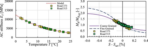
For the backcalculation procedure, the cross-sections of the structures were divided into sublayers. This was done to take into account the variation in moisture levels and whether the part of the structure during the measurements was frozen or thawed. For both structures, the frozen part of the cross-section was estimated at the time of measurement which is marked by a dotted line in Figures 6 and 7. In the case of Lv515, the subgrade was considerably thick and a large variation in moisture was recorded by the TDR probes. The volumetric moisture content values recorded by the TDR probes were converted into the degree of saturation and then implemented in the model. The default model parameters for coarse-grained material were used, a = −0.3123, b = 0.3, and k_s= 6.8157 (ARA Inc. 2004). Two different optimal resilient moduli (M_r,opt) as 90 and 85 MPa and the optimal degree of saturation (S_opt) values were used as 20% and 15%, respectively. The higher values for the undisturbed material outside the trench are due to the higher degree of compaction.

The backcalculation was performed iteratively. An initial set of layer stiffness values were assumed. To quantify and minimise the difference between the measured and the calculated values, the root mean square error RMSE was used (3) $\mathrm{RMSE}=\sqrt{{\displaystyle \frac{\sum _{i=1}^n{(y_i-\hat{y})}^2}{n}}}$(3) where y_i represents a measured datapoint, ŷ a calculated datapoint, and n is the total number of datapoints.

Three RMSE values were defined for the error minimisation procedure. The first RMSE value was used to compare the surface deflections measured by the FWD to the calculated surface deflections by MLET at those locations. The typical RMSE values for the FWD backcalculation were in the range of 3–5 with the exception of the backcalculation for road 515 during the August 2019 campaign which had an RMSE value of 11. The second RMSE value was used to compare the stress and strain values recorded by the ASGs, ϵMU coils, and SPCs to the MLET-calculated stress and strain values at the known location of each respective type of sensor. Typical RMSE values for individual built-in sensor response under FWD loading range between 6 and 12. The third RMSE value was obtained through the difference between the assumed M_r – recorded degree of saturation values and the M_r-moisture model. The values of the RMSE used to adjust for the temperature and moisture variations ranged between 1 and 4. The stiffness values at the dates of measurements obtained through the iterative procedure are given in Tables 1 and 2.

Table 1. Backcalculated stiffness values at each measurement date for Lv373. Out. and In. represent the value sets outside and inside the trench.

Layer	Thickness	Stiffness (MPa)
		29 August 2018		8 May 2019		12 June 2019		21 August 2019
	(cm)	Out.	In.	Out.	In.	Out.	In.	Out.	In.
1. Asphalt Concrete	10	6107	6107	10,756	10,756	4464	4464	5764	5764
2. Base Course	12	383	341	376	336	331	296	380	329
3. Subbase	26	266	197	259	191	256	187	248	177
4. Base Course	12	169	118	166	116	147	102	154	103
5. Tarmac	13	149	138	232	201	158	152	188	182
6. Subbase	30	148	88	143	84	169	101	161	97
7. Sandy Clay	15	129	76	117	71	133	79	131	77
8. Subgrade (dfrost)	42	64	51	2800	2800	49	39	47	37
9. Subgrade (dfrost)	45	74	74	2800	2800	2800	2800	68	68
10. Subgrade Unfrozen	∞	75	75	105	105	72	72	76	76

Table 2. Backcalculated stiffness values at each measurement date for Lv515. Out. and In. represent the value sets outside and inside the trench.

Layer	Thickness	Stiffness (MPa)
		30 August 2018		9 May 2019		13 June 2019		22 August 2019
	(cm)	Out.	In.	Out.	In.	Out.	In.	Out.	In.
1. Asphalt Concrete	4	5160	5160	10,421	10,421	4605	4605	6138	6138
2. UGM Base	15	180	145	150	135	195	160	185	155
3. SG Sub.1 (TDR1)	37	93	76	90	74	100	82	97	78
4. SG Sub.2 (TDR2)	40	94	78	91	76	106	86	98	82
5. SG Sub.3 (TDR3)	40	85	73	78	69	95	80	89	75
6. SG Sub.4(TDR4,dfrost)	14	77	67	2800	2800	83	73	77	67
7. SG Sub.5 (dfrost,June)	10	85	85	2800	2800	2800	2800	87	87
8. SG Sub.6	16	95	95	2800	2800	2800	2800	97	97
9. SG Sub.7 (TDR5,dfrost)	84	107	107	2800	2800	2800	2800	108	108
10. SG Sub.8 (Natural SG)	∞	107	107	95	95	96	96	108	108

Both structures were partially frozen during the May and June measurement campaigns. This has been considered in the backcalculation procedure according to the depth interval where the frozen part of the cross-section was located (d_frost). For Lv373 it was possible to capture the upper boundary of the frozen part of the cross-section but not the full extension of the frozen part. For Lv515 it was possible to capture the upper boundary of the frozen part only during the May campaign. For the June campaign at Lv515, it was not possible to capture neither the upper nor the lower depth of the frozen part. This was due to the 200 cm limited length of the frost rods. The values of the frost depth were obtained through a statistical-based empirical correlation developed for the conditions in Sweden, in which the frost penetration depth is obtained as a function of the freezing index determined by air temperature registrations at a specific location (Erlingsson and Saliko 2020). The empirical values were used as an initial estimate which was further refined by interpolating the slope of the seasonally frozen zone from Figures 6 and 7. The stiffness of the frozen layer was set to 2800 MPa which is in agreement with previous studies (Salour and Erlingsson 2013b).

Vehicle response modelling

The response of the structure under loading by LHVs was measured at each testing campaign afterwards performing the FWD testing. Three different types of LHVs were used, one of which is shown in Figure 11. The loading was applied by driving the vehicles at a constant speed of 60 km/h (50 km/h at Lv515 in May 2019) over the sensors in a way that the outer wheels would be aligned along the wheel path directly on top of the built-in sensors. The location of the sensors had previously been marked on the surface.

Figure 11. The LHV2 used for the response measurements. The axles are shown according to the used naming convention.

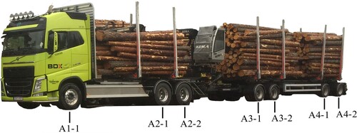
The configuration of vehicle loading (single vs. dual tyres, tyre pressures, number of axles, load per axle, total load, and total length) was different for each of the three LHVs used. LHV1 had 9 axles, two of them having single tyres and seven with dual tyres, with a total length centre-to-centre of the first to the last axle of 20.5 m and a total weight of approximately 74 tons. LHV2 had seven axles, the driving axle with single tyres while the rest of the axles had dual tyre configuration. The centre-to-centre length between the first and last axle for LHV2 was 19.74 m and the total weight was approximately 64 tons. LHV3 had eight axles, seven of them with single tyres and one with dual tyres, an axle centre-to-centre total length of 20.8 m, and a total weight of approximately 68 tons.

A naming convention was established to identify each type of LHVs as well as individual axles and axle groups. Axles located close to each other are considered to belong to the same axle group. The ID assigned to an axle represents first the axle group and then the number of the axle within that group. The axle configurations, identification names, and axle spacing in centimetres for all three LHVs are shown in Figure 12. Before each testing campaign, the axle weights were measured by static weighing each LHV and the tyre pressures were measured using a regular tyre pressure gauge. The axle weights and tyre pressures for each axle are shown in Table 3.

Figure 12. Half-axle and tyre configuration, spacing, and IDs for the LHVs used in this study. All distances in cm.

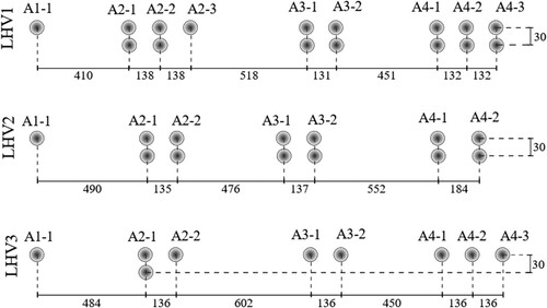
Table 3. Measured axle loads F and tyre pressures p for the three LHVs used in the study. Type S and D represent single vs. dual tyres respectively.

Axle	LHV1			LHV2			LHV3
ID	Type	p	F	Type	p	F	Type	p	F
(–)	(–)	(kPa)	(kN)	(–)	(kPa)	(kN)	(–)	(kPa)	(kN)
A1-1	S	840	83.36	S	850	74.53	S	890	93.16
A2-1	D	750	83.85	D	700	93.65	D	700	114.25
A2-2	D	750	82.38	D	700	91.20	S	920	67.67
A2-3	S	840	65.70	–	–	–	–	–	–
A3-1	D	850	87.77	D	900	91.20	S	870	94.14
A3-2	D	850	90.22	D	900	89.73	S	860	95.61
A4-1	D	850	78.45	D	900	101.50	S	870	69.14
A4-2	D	850	79.43	D	900	100.03	S	890	72.08
A4-3	D	850	80.41	–	–	–	S	890	74.53
ΣF			731.58			641.85			680.58

The LHV1 had the lowest variation in axle loads, the lowest calculated average value of axle load and the lowest tyre pressure, despite having the highest total weight. LHV2 had the highest average axle load since the weight was distributed over a lower number of axles compared to the two other vehicles. For LHV3 multiple single tyres were used in the axel configuration. The largest load for a single axle was measured in the case of LHV3.

Results of the vehicle induced response

For the calculations of the structural response of the test sections under moving load by the LHVs, the MLET-based software ERAPave (Erlingsson and Ahmed 2013; Saevarsdottir et al. 2016; Ahmed and Erlingsson 2017) was used. The stiffness values of the AC layers were adjusted for the temperature at the time of testing and the stiffness values of the UGM layers were adjusted according to the moisture levels (Tables 1 and 2). The loading was modelled according to Table 3 and Figure 12 except to simplify the modelling process and to lower the computational time, the tyre pressure was considered constant at 850 kPa for all tyres which is close to the average of all the tyre pressures. A sensitivity analysis on the influence of the variation of tyre pressure was performed which showed that the impact of different tyre pressures is negligible for the range of the tested vehicles. The details of the sensitivity analysis have been omitted due to space and scope limitations. Any minor differences in driving speed and positioning in transversal direction due to human error in driving were neglected.

Comparisons between the measured and calculated responses from the structures are shown in Figures 13–19. As shown, the strain registrations from the longitudinal ASGs exhibit the lowest difference between the measured response signals and the MLET calculations. The accuracy was lower in the case of transversal ASGs as can be inferred from Figures 14 and 17. It was observed that the ASGs placed in the transversal direction were sensitive to the lateral position of the axle applying the load. Small lateral deviations in the load application led to measured values that were lower than the expected values. Depending on the position of the axle applying the load, different parts of the registration curves matched the calculations. In cases when the first wheel was positioned correctly, the first peak of the registered curve corresponding to the driving axle matched the calculations as shown in Figure 14(a). In cases when the driver adjusted the positioning near the end of the time when the truck was passing on top of the sensors, the last peaks of the registration corresponding to the trailer axles matched the calculations as shown in Figure 14(b). In the case of ASGs, not considering whether their placement is longitudinal or transversal, the sensors can successfully capture the structural behaviour of the pavement in case the loading is applied at the correct position.

Figure 13. Longitudinal horizontal strain ϵ_xx response registrations from ASG compared to MLET calculations at Lv373 under LHV1 for (a) August 2018, (b) May 2019, (c) June 2019, and (d) August 2019.

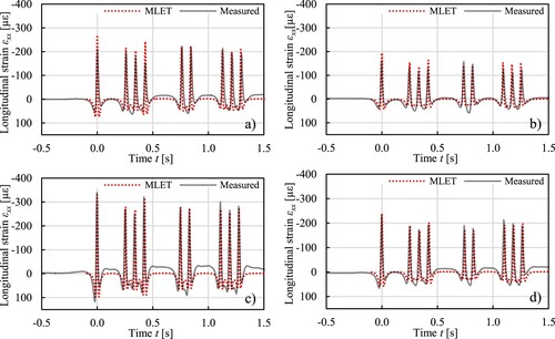
Figure 14. Transversal horizontal strain ϵ_yy response registrations from ASG compared to MLET calculations at Lv373 under LHV2 for (a) August 2018, (b) May 2019, (c) June 2019, and (d) August 2019.

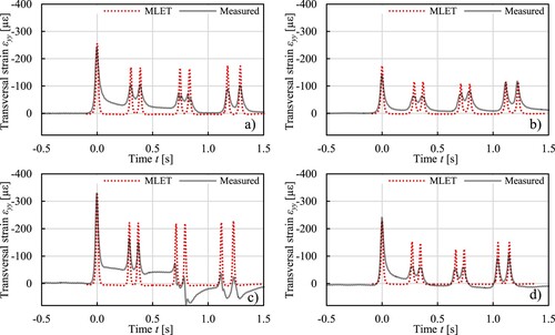
Figure 15. Vertical stress σ_zz response registrations from SPC at 35 cm depth compared to MLET calculations at Lv373 under LHV3 for (a) August 2018, (b) May 2019, (c) June 2019, and (d) August 2019.

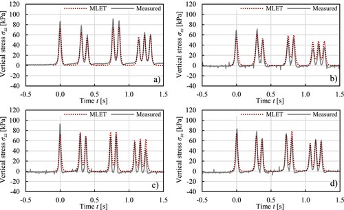
Figure 16. Longitudinal horizontal strain ϵ_xx response registrations from ASG compared to MLET calculations at Lv515 under LHV1 for (a) August 2018, (b) May 2019, (c) June 2019, and (d) August 2019.

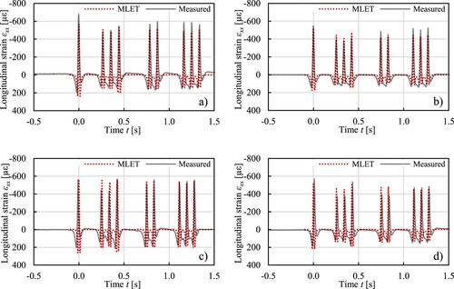
Figure 17. Transversal horizontal strain ϵ_yy response registrations from ASG compared to MLET calculations at Lv515 under LHV2 for (a) August 2018, (b) May 2019, (c) June 2019, and (d) August 2019.

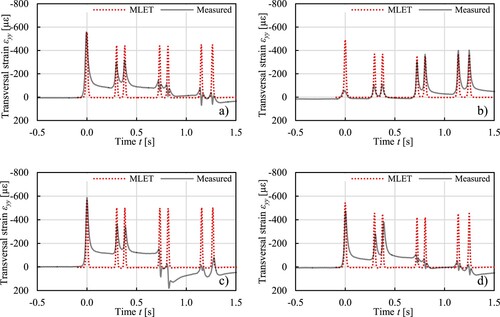
Figure 18. Vertical stress σ_zz response registrations from SPC at 38 cm depth compared to MLET calculations at Lv515 under LHV3 for (a) August 2018, (b) May 2019, (c) June 2019, and (d) August 2019.

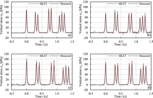
Figure 19. Vertical strain ϵ_zz response registrations from ϵMU coil at 84 cm depth compared to MLET calculations at Lv515 under LHV1 for (a) August 2018, (b) May 2019, (c) June 2019, and (d) August 2019.

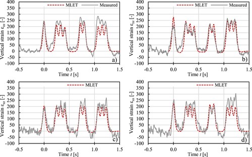
The vertical strain signals recorded by the ϵMU coils were noisier compared to the other types of sensors, in particular in the case of Lv373 which consisted of several layers. These sensors were also observed to be the least durable. For Lv373, the two bottom ϵMU coils from one of the trenches were malfunctioning during three out of the four testing campaigns. For Lv515, the uppermost ϵMU coil from one of the trenches malfunctioned during the May 2019 campaign which increased to three ϵMU coils malfunctioning during the measurements of August 2019.

The stresses measured by the SPCs showed reasonable prediction accuracy. The vertical stresses recorded by the SPCs located in the upper part of the structure were found to depend more on the temperature of the AC layer than the moisture of the UGM layers in which they were located. The environmental-related variables such as the temperature of the AC and the moisture of the UGM layers did not have a large effect on the vertical stresses recorded by the SPCs located at deeper layers. Instead, the properties of the loading configurations such as the axle load, and tyre configuration (single vs. dual tyres) were found to have the main influence.

The vertical strains recorded by the ϵMU coils showed noisier signals compared to the other types of sensors. However, in most cases, the measured values fitted adequately with the calculated values. Deviations were noticed mainly for the three last peaks that correspond to the strains caused by the last tridem trailer axle of the LHV1 as shown in Figure 19(c,d) for the ϵMU at 76 cm depth. The increase in strains under loading by the last tridem axle was observed mainly in combination with increased moisture content in the structure. This was observed only for LHV1 and not for the other two vehicles. The exact reason for this is unknown. A possible hypothesis is that the increase in measured strains comes due to a local temporary pore water pressure build-up that dissipates afterwards.

For the comparison between the measurement campaigns, the peak strain values from the longitudinal ASGs were taken into consideration. These sensors were selected as they offered the highest reliability. The lowest strains under the AC layer for both structures were recorded during the May 2019 measurement campaign. During the May 2019 campaign, the temperature of the AC layer was the lowest compared to the other measurement campaigns. The highest temperature and the highest longitudinal strains under the AC layer were recorded during the June 2019 campaign. Similar temperature values were recorded for the August 2018 and August 2019 measurement campaigns, however, some differences in strain values were observed. For the August 2019 campaign, the recorded AC temperature was slightly lower, but the moisture recorded by TDR1 at 36 cm depth was lower than in the August 2018 measurement campaign. This is an indicator that the strains at the bottom of the AC layer depend not only on the stiffness of the AC layer but also on the support from the granular base course under the asphalt.

Comparisons between multilayer linear and nonlinear modelling

The comparison between the measured response and numerical calculations using linear MLET-based software showed a good fit, indicating that the linear elastic theory is a suitable method for the response modelling. However, the viscoelastic behaviour of the asphalt layers and the stress-dependent nonlinear behaviour of the UGM layers is therefore neglected. To further investigate the significance of the abovementioned factors, two additional modelling approaches were set up for comparisons, that is assuming, the AC layers exhibit a viscoelastic behaviour, but all other layers are linear elastic materials, and thereafter that the UGM (base course and subbase) were modelled as stress-dependent linear elastic materials but the asphalt layers and the subgrade were modelled as linear elastic materials. As before the ERAPave software was used. A detailed description of the approach can be found in Ahmed and Erlingsson (2017). The approach is based on the elastic-viscoelastic correspondence principle in which the Laplace transform of the constitutive equations for linear viscoelastic problems is formulated similarly to homogenous and isotropic linear elastic problems (Huang 2004; Kim 2011). The creep compliance of the asphalt materials is therefore required as an input for the viscoelastic modelling. A power function derived from complex modulus (Baumgaertel and Winter 1989; Tschoegl 2012) was used for the viscoelastic modelling of the asphalt layer. (4) $\begin{array}{c}\begin{array}{c}D(t)=D_0+D_1{t}^m\\ D^{\mathrm{\prime }}(\omega )=D_0+D_1\mathrm{\Gamma }(m+1){\omega }^{-m}\cos (m\pi (2k+1/2))\end{array}\\ D^{\mathrm{\prime }\mathrm{\prime }}(\omega )=D_1\mathrm{\Gamma }(m+1){\omega }^{-m}\sin (m\pi (2k+1/2))\\ k=0,\pm 1,\pm 2\dots \end{array}$(4) where D´(ω) is the storage creep compliance, D″(ω) is the loss creep compliance, ω is the frequency, Γ is the gamma function, and D₀, D₁, and m are the parameters for the power function creep compliance curve.

For the power function of the creep compliance curve, the parameters were taken from a previous study D₀=  1.47E-07, D₁=  1.27E-03, and m = 0.06 (Ahmed and Erlingsson 2016).

To model the stress-dependent nonlinear behaviour in the granular layers, the k-θ model (Uzan 1985; Lekarp et al. 2000; Leischner 2016) expressed in a normalised form was used. (5) $M_r=k_1{p}_a{\left({\displaystyle \frac{3p}{p_a}}\right)}^{k_2}$(5) where k₁ and k₂ are model constants derived experimentally, p is the mean normal stress equal to 1/3 of the sum of the principal stresses, and p_a is the reference pressure at 100 kPa.

The model has been shown to capture the response of UGMs when subjected to rolling wheel loading (Erlingsson 2010; Saevarsdottir and Erlingsson 2015). The constants used in the modelling process were taken from previous studies as k₁= 900, and k₂= 0.4 (Tseng and Lytton 1989; Rahman and Erlingsson 2015).

The comparison was made for the August 2018 measurement campaign at Lv515 subjected to loading by LHV1 between two selected measurements and the corresponding calculations. The comparisons were made for the longitudinal strain under the AC layer recorded by the ASG at 4 cm depth as shown in Figure 20(a) and for the vertical stress recorded by the SPCs at 38 cm depth as shown in Figure 20(b). The bottom of the AC layer and the top of the subgrade were selected as they are known to be locations where critical strains in the structure occur.

Figure 20. Comparison between measured responses, linear elastic modelling (LE), viscoelastic modelling (VE), and nonlinear k-theta modelling (k-theta) for (a) longitudinal asphalt strain gauge ASG, and (b) soil pressure cell SPC under LHV1 in measurements in August 2018.

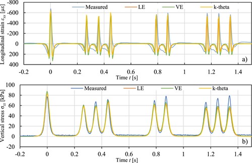
Based on the comparison shown in Figure 20, minor differences were found between the calculated responses by the linear elastic, viscoelastic, and the k-θ model. The viscoelastic and the k-θ model were found to offer an improvement in the range of 1–4% over the linear elastic model in the prediction of the response peaks shown in Figure 20. The temperatures during the times when the response testing was performed were relatively low, which has led to a less pronounced viscoelastic behaviour of the AC. Due to the abovementioned reasons, it was decided to continue with linear elastic modelling due to its simplicity and faster computational time which would also be an advantage later for performance prediction calculations. In other scenarios at higher temperatures and larger loading magnitude variations, it would be relevant to look further into the effect of the viscoelasticity of the asphalt and the nonlinear behaviour of the granular materials.

Evaluation of the modelling accuracy

To evaluate the accuracy of the modelling by MLET, the peaks of the measured curves for each of the sensor types were compared against the calculated peak values. The comparison is illustrated in Figure 21. Each data point shown in the plot corresponds to one peak of the response curves obtained by the loading of one axle of a specific LHV. The plot includes the peaks from the response of all three types of LHVs. The results are grouped based on the section corresponding to where the measurements were made. To statistically quantify the accuracy of the fit, the coefficient of determination R² and the normalised root mean square error NRMSE were used. The NRMSE was defined as (4) $\mathrm{NRMSE}={\displaystyle \frac{\mathrm{RMSE}}{y_{max}-y_{min}}}$(4) where y_max represents the largest measured datapoint, and y_min represents the smallest measured datapoint.

Figure 21. Validation of calculations against measurements for (a) longitudinal ASGs, (b) transversal ASGs, (c) SPCs, and (d) EMUs for all four measurements campaigns.

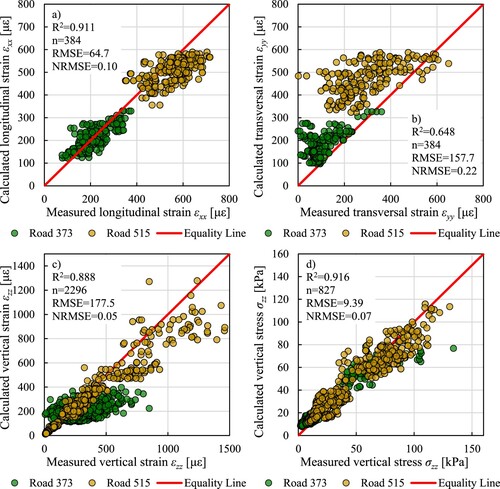
The NRMSE was used to facilitate the comparison between datasets of different scales. The number of data points n,the R² value, and the NRMSE value are given in the plots.

As shown in Figure 21, the best fit between the measured and calculated values indicated by a higher R² value and lower NRMSE was obtained in the case of the longitudinal horizontal strain ϵ_xx from the ASGs and the vertical stress σ_zz from the SPCs. A slightly higher R² value was calculated for the SPCs due to the spread of the data points over a wider range as the sensors were located at multiple depths compared to the longitudinal ASGs which were located at a single depth. For the longitudinal strains, two separate clusters corresponding to each of the sections are observed. This is due to the difference in AC layer thickness between the two sections, higher strains occur in the case of Lv515 due to the lower thickness of the AC layer.

The highest NRMSE value, lowest R² value and lowest prediction accuracy were estimated in the case of the transversal horizontal strains ϵ_yy recorded by transversal ASGs. The measured values for this type of sensor were lower compared to the calculated values due to difficulties in maintaining the correct lateral position during the testing campaigns. This is an indicator that the response and usability of this type of sensor highly depend on the correct positioning of the vehicle in the transversal direction during the testing. This also indicates that in most cases there will be a lateral wander when the vehicles pass above the structure. This could lead to fatigue performance estimates to be on the conservative side, as typically they assume that the loading follows the wheel path.

A high R² value of 0.888 was calculated in the case of the ϵMU coils. The NRMSE value for the ϵMU coils was calculated to be 0.05. When looking at individual sensor responses for Lv373 some deviations between the measured and calculated values were observed for the ϵMU sensors that were located between two layers. This occurred in the cases when a layer was thin and it was not possible to place the ϵMU coil sensor only within that layer. This is shown in Figure 21(c) where the points representing Lv373 show a larger scatter compared to the points representing Lv515. However, the spread of the ϵMU coil sensors over a large range of depths led to a high calculated R² value.

Conclusions

Two thin pavement structures located in the northern part of Sweden have been instrumented with road response and climatic sensors. Registrations from LHV passes at normal speed have been gathered during different seasons. The readings have further been compared with the results from numerical calculations using MLET-based software.

ASGs, SPCs and ϵMU coils were successfully used to provide induced response data throughout different seasons under loading from LHVs. The variation of the temperature, moisture content, and frost penetration in the cross-section of the pavement structures was monitored successfully by thermocouples (temperature in the AC layer), moisture rod (moisture variation in the granular layers), and frost rod (temperature granular layers).

The data obtained from environmental sensors was used together with the FWD backcalculation to obtain layer stiffness values. The backcalculated stiffness values were thereafter used as input for the linear MLET-based response modelling. The MLET numerical simulation due to the three LHV´s loadings where the material properties of the pavement layers were updated according to the environmental readings gave good results. The modelling was relatively accurate, this was true for both the late summer measurements as well as during the spring thaw period. This is essential in order to use the method in an M-E calculation scheme.

The longitudinal tensile strains at the bottom of the asphalt layer were primarily influenced by the temperature of the asphalt layer, with lower recorded strains at low temperatures. Increased moisture content in the unbound granular material leads to lower stiffness of unbound granular layers and increasing longitudinal tensile strains.

Comparisons of measured and calculated longitudinal horizontal strains and vertical stresses and strains gave high coefficients of determination R². The transversal horizontal strain calculations gave slightly higher values than the measured ones reducing the coefficient of determination. The transversal horizontal strains are however highly dependent on the lateral position of the applied load. As it was not possible to keep a correct positioning, lower registered values were observed compared to the calculated values as expected.

Minor reliability issues occurred with the ϵMU coils in some of the testing campaigns due to malfunctions. The registrations from the ϵMU coil sensors were noisier compared to the other types and in some cases stopped functioning. The reliability of the configuration could be improved by increasing the number of ϵMU coils or by using more durable sensors. Further improvements could be made in the response capturing accuracy by adding more ASGs in the transversal direction to account for the lateral deviations in vehicle positioning.

Non-linear MLET including viscoelastic behaviour of the asphalt layers or stress dependency of the granular layers only marginally improved the calculations compared to the linear MLET solutions. It was therefore concluded to include the linear MLET-based approach in the new M-E design and prediction tool that is under development in Sweden using a climatic model to adjust the stiffness properties of the different pavement layers. The response validation carried out in this study was performed only at two locations for a limited range of temperatures and loading magnitudes. The effects of higher temperatures and larger loading magnitudes should be further studied in order to investigate the impact of the viscoelasticity of the AC layers and the nonlinear behaviour of the granular materials.

Disclosure statement

No potential conflict of interest was reported by the author(s).

Additional information

Funding

This work was supported by Trafikverket.

References

- Ahmed, A. and Erlingsson, S., 2013. Evaluation of permanent deformation models for unbound granular materials using accelerated pavement tests. Road Materials and Pavement Design, 14 (1), 178–195. doi:10.1080/14680629.2012.755936.
- Ahmed, A. and Erlingsson, S., 2016. Viscoelastic response modelling of a pavement under moving load. Transportation Research Procedia, 14, 748–757. doi:10.1016/j.trpro.2016.05.343.
- Ahmed, A.W. and Erlingsson, S., 2017. Numerical validation of viscoelastic responses of a pavement structure in a full-scale accelerated pavement test. International Journal of Pavement Engineering, 18 (1), 47–59. doi:10.1080/10298436.2015.1039003.
- Al-Qadi, I.L., et al., 2004. The Virginia smart road: the impact of pavement instrumentation on understanding pavement performance. Journal of the Association of Asphalt Paving Technologists, 73 (3), 427–465.
- Andrei, D., Witczak, M.W., and Houston, W.N., 2009. Resilient modulus predictive model for unbound pavement materials. In: Contemporary topics in ground modification, problem soils, and geo-support. 401–408. doi:10.1061/41023(337)51.
- ARA Inc., 2004. Guide for mechanistic–empirical design of new and rehabilitated pavement structures. Final Rep., NCHRP Project 1-37A. Available from: https://onlinepubs.trb.org/onlinepubs/archive/mepdg/guide.htm.
- Baumgaertel, M. and Winter, H.H., 1989. Determination of discrete relaxation and retardation time spectra from dynamic mechanical data. Rheologica Acta, 28 (6), 511–519. doi:10.1007/BF01332922.
- Blanc, J., et al., 2019. Monitoring of an experimental motorway section. Road Materials and Pavement Design, 20 (1), 74–89. doi:10.1080/14680629.2017.1374997.
- Burmister, D.M., 1945. The general theory of stresses and displacements in layered systems. I. Journal of Applied Physics, 16 (2), 89–94. doi:10.1063/1.1707558.
- Christidis, P. and Leduc, G., 2009. Longer and heavier vehicles for freight transport. JRC 52005. European Commission, Joint Research Centre, Institute for Prospective Technological Studies, 1–40. Available from: https://ec.europa.eu/transport/sites/transport/files/modes/road/events/doc/2009_06_24/2009_jrc52005.pdf.
- Doré, G. and Zubeck, H.K., 2009. Cold regions pavement engineering. Reston, VA: New York: ASCE Press; McGraw-Hill. 978-0-07-160088-0.
- Duong, N.S., et al., 2019. Continuous strain monitoring of an instrumented pavement section. International Journal of Pavement Engineering, 20 (12), 1435–1450. doi:10.1080/10298436.2018.1432859.
- Erlingsson, S., 2010. Impact of water on the response and performance of a pavement structure in an accelerated test. Road Materials and Pavement Design, 11 (4), 863–880. doi:10.1080/14680629.2010.9690310.
- Erlingsson, S., 2012. Rutting development in a flexible pavement structure. Road Materials and Pavement Design, 13 (2), 218–234. doi:10.1080/14680629.2012.682383.
- Erlingsson, S. and Ahmed, A., 2013. Fast layered elastic response program for the analysis of flexible pavement structures. Road Materials and Pavement Design, 14 (1), 196–210. doi:10.1080/14680629.2012.757558.
- Erlingsson, S., Rahman, M.S., and Ahmed, A., 2018. Impact of longer and heavier vehicles on the performance of asphalt pavements: A laboratory study. In: A. Loizos, I.L. Al-Qadi, and A. (Tom) Scarpas, eds. Bearing capacity of roads, railways and airfields. 1st ed. CRC Press, 483–490. doi:10.1201/9781315100333-63.
- Erlingsson, S., Rahman, S., and Salour, F., 2017. Characteristic of unbound granular materials and subgrades based on multi stage RLT testing. Transportation Geotechnics, 13, 28–42. doi:10.1016/j.trgeo.2017.08.009.
- Erlingsson, S. and Saliko, D., 2020. Correlating air freezing index and frost penetration depth – a case study for Sweden. In: C. Raab, ed. Proceedings of the 9th international conference on maintenance and rehabilitation of pavements – Mairepav9. Vol. 76. Springer International Publishing, 847–857. doi:10.1007/978-3-030-48679-2_79
- Fladvad, M. and Erlingsson, S., 2022. Modelling the response of large-size subbase materials tested under varying moisture conditions in a heavy vehicle simulator. Road Materials and Pavement Design, 23 (5), 1107–1128. doi:10.1080/14680629.2021.1883462.
- Gkyrtis, K., Armeni, A., and Loizos, A., 2021. A mechanistic perspective for airfield pavements evaluation focusing on the asphalt layers’ behaviour. International Journal of Pavement Engineering, 1–14. doi:10.1080/10298436.2021.1995733.
- Gusfeldt, K.H. and Dempwolff, K.R., 1967. Stress and strain measurements in experimental road sections under controlled loading conditions. 2nd international conference on the structural design of asphalt pavements. Ann Arbor, Michigan. 663–669.
- Hicks, R.G. and Finn, F.N., 1970. Analysis of results from the dynamic measurements program on the San Diego test road. Association of Asphalt Paving Technologists, 39, 153–185. Available from: https://trid.trb.org/view/101320.
- Huang, Y.H., 2004. Pavement analysis and design. 2nd ed Upper Saddle River, NJ: Pearson/Prentice Hall. 978-0-13-142473-9.
- Irwin, L.H., 2002. Backcalculation: an overview and perspective. In: Pavement evaluation conference, 2002, Roanoke, VI.
- Kim, J., 2011. General viscoelastic solutions for multilayered systems subjected to static and moving loads. Journal of Materials in Civil Engineering, 23 (7), 1007–1016. doi:10.1061/(ASCE)MT.1943-5533.0000270.
- Knight, I., et al., 2008. Longer and/or longer and heavier goods vehicles (LHVs) – a study of the likely effects if permitted in the UK: final report. TRL Limited. Available from: http://data.parliament.uk/DepositedPapers/Files/DEP2008-1410/DEP2008-1410.pdf.
- Leischner, S., et al., 2016. Design of thin surfaced asphalt pavements. Procedia Engineering, 143, 844–853. doi:10.1016/j.proeng.2016.06.138.
- Lekarp, F., Isacsson, U., and Dawson, A., 2000. State of the Art. II: permanent strain response of unbound aggregates. Journal of Transportation Engineering, 126 (1), 76–83. doi:10.1061/(ASCE)0733-947X(2000)126:1(76).
- Leong, E.C. and Rahardjo, H., 1997. Review of soil-water characteristic curve equations. Journal of Geotechnical and Geoenvironmental Engineering, 123 (12), 1106–1117.
- Loulizi, A., Al-Qadi, I.L., and Elseifi, M., 2006. Difference between in situ flexible pavement measured and calculated stresses and strains. Journal of Transportation Engineering, 132 (7), 574–579.
- Natanaelsson, K. and Eriksson, T., 2020. Regeringsuppdrag: Implementering av bärighetsklass 4. Trafikverket, TRV 2020/44448. In Swedish.
- Ortega, A., et al., 2014. Are longer and heavier vehicles (LHVs) beneficial for society? A cost benefit analysis to evaluate their potential implementation in Spain. Transport Reviews, 34 (2), 150–168. doi:10.1080/01441647.2014.891161.
- Pålsson, H., et al., 2017. Longer and heavier road freight vehicles in Sweden: effects on tonne- and vehicle-kilometres, CO2 and socio-economics. International Journal of Physical Distribution & Logistics Management, 47 (7), 603–622. doi:10.1108/IJPDLM-02-2017-0118.
- Pereira, P. and Pais, J., 2017. Main flexible pavement and mix design methods in Europe and challenges for the development of an European method. Special Issue on Maintenance and Rehabilitation of Pavements, 4 (4), 316–346. doi:10.1016/j.jtte.2017.06.001.
- Rahman, M.S. and Erlingsson, S., 2015. Predicting permanent deformation behaviour of unbound granular materials. International Journal of Pavement Engineering, 16 (7), 587–601. doi:10.1080/10298436.2014.943209.
- Saevarsdottir, T. and Erlingsson, S., 2015. Modelling of responses and rutting profile of a flexible pavement structure in a heavy vehicle simulator test. Road Materials and Pavement Design, 16 (1), 1–18. doi:10.1080/14680629.2014.939698.
- Saevarsdottir, T., Erlingsson, S., and Carlsson, H., 2016. Instrumentation and performance modelling of heavy vehicle simulator tests. International Journal of Pavement Engineering, 17 (2), 148–165. doi:10.1080/10298436.2014.972957.
- Saliko, D. and Erlingsson, S., 2021. Damage investigation of thin flexible pavements to longer heavier vehicle loading through instrumented road sections and numerical calculations. Road Materials and Pavement Design, 22 (sup1), S575–S591. doi:10.1080/14680629.2021.1899964.
- Salour, F., 2015. Moisture influence on structural behaviour of pavements: field and laboratory investigations. PhD thesis. Architecture and the Built Environment, KTH Royal Institute of Technology. Available from: https://www.diva-portal.org/smash/get/diva2:796833/SUMMARY01.pdf.
- Salour, F. and Erlingsson, S., 2013a. Moisture-sensitive and stress-dependent behavior of unbound pavement materials from in situ falling weight deflectometer tests. Transportation Research Record: Journal of the Transportation Research Board, 2335 (1), 121–129. doi:10.3141/2335-13.
- Salour, F. and Erlingsson, S., 2013b. Investigation of a pavement structural behaviour during spring thaw using falling weight deflectometer. Road Materials and Pavement Design, 14 (1), 141–158. doi:10.1080/14680629.2012.754600.
- Sanchez Rodrigues, V., et al., 2015. The longer and heavier vehicle debate: a review of empirical evidence from Germany. Transportation Research Part D: Transport and Environment, 40, 114–131. doi:10.1016/j.trd.2015.08.003.
- Simonsen, E. and Isacsson, U., 1999. Thaw weakening of pavement structures in cold regions. Cold Regions Science and Technology, 29 (2), 135–151. doi:10.1016/S0165-232X(99)00020-8.
- Terrell, R.L. and Krukar, M., 1970. Evaluation of-test tracking pavements. Association of Asphalt Paving Technologists, 39, 273–296.
- Tschoegl, N.W., 2012. The phenomenological theory of linear viscoelastic behavior: an introduction. Cham: Springer Science & Business Media.
- Tseng, K.-H. and Lytton, R., 1989. Prediction of permanent deformation in flexible pavement materials. In: H. Schreuders and C. Marek, eds. Implication of aggregates in the design, construction, and performance of flexible pavements. ASTM International, 154–172. doi:10.1520/STP24562S.
- Uzan, J., 1985. Characterization of granular materials. Transportation Research Board, 1022. Available from: http://onlinepubs.trb.org/Onlinepubs/trr/1985/1022/1022-007.pdf.