Evaluation of Methods for Viscosity Simulations of Lubricants at Different Temperatures and Pressures: A Case Study on PAO-2

Abstract

The behavior of lubricants at operational conditions, such as at high pressures, is a topic of great industrial interest. In particular, viscosity and the viscosity-pressure relation are especially important for applications and their determination by computational simulations is very desirable. In this study, we evaluate methods to compute these quantities based on fully atomistic molecular dynamics simulations, which are computationally demanding but also have the potential to be most accurate. We used the 9,10-dimethyloctadecane molecule, main component of PAO-2 base oil as the lubricant for our tests. The methods used for the viscosity simulations are the Green-Kubo equilibrium molecular dynamics (EMD-GK) and nonequilibrium molecular dynamics (NEMD), at pressures of up to 1.0 GPa and various temperatures (40-150 degrees Celsius). We present the theory behind these methods and investigate how the simulation parameters affect the results obtained, to ensure viscosity convergence with respect to the simulation intervals and all other parameters. We show that, by using each method in its regime of applicability, we can achieve good agreement between simulated and measured values. NEMD simulations at high pressures captured zero shear viscosity successfully; while at 40 degrees Celsius, EMD-GK is only applicable to pressures up to 0.3 GPa, where the viscosity is lower. In NEMD, longer and multiply repeated simulations improve the confidence interval of viscosity, which is essential at lower pressures. Another aspect of these methods is the choice of the utilized force field for the atomic interactions. This was investigated by selecting two different commonly used force fields.

Keywords:

• Non-Newtonian behavior
• viscosity-pressure
• viscosity-temperature
• synthetic base stocks
• lubricant physical analysis

Introduction

Lubricants are of great importance and extensively used in the industry, where there is a constant effort to increase the efficiency and lifetime of tribological systems, while combining the best possible material characteristics. Over the past 30 years, the interest in obtaining viscosity values from a simulation at various operational conditions (temperatures, pressures, shear rates) has risen sharply. This is due to the fact that computer simulations with the use of molecular dynamics and other methods can provide useful and valuable insights in cases where measuring rheological properties can be difficult or not possible at all. There has been extensive work (1) for calculating key lubricant properties (density, viscosity) with molecular dynamics at ambient conditions, for various hydrocarbon lubricants, including linear and branched alkanes. Simulated and experimental values were very close in certain cases. Additionally, work has been done (2) on which model is most appropriate for lubricants by comparing classical force fields for molecular dynamics simulations. The results showed that the L-OPLS-AA (all-atom model for long hydrocarbons) gave better viscosity estimates, when equilibrium molecular dynamics were used for calculating the above-mentioned properties. The general tendency is that, at the cost of computation time, all-atom models, which describe each atom explicitly, perform significantly better than united atom models (3), where the nonpolar hydrogens are grouped with the carbon atoms to generate CH, CH₂ and CH₃ pseudo-atoms. Molecular dynamics simulations coupled with the pioneering Green-Kubo method (4, 5), appear to be efficient at low viscosity values and ambient conditions (6, 7). This method uses internal equilibrium fluctuations, by evaluating integrals of autocorrelation functions, to describe transport properties such as zero shear (low shear) viscosity. However, some accuracy issues have been raised at high viscosities, and alternative methods such as nonequilibrium molecular dynamics (NEMD) (8, 9) or reverse nonequilibrium molecular dynamics (RNEMD) (10) have been proposed as the current state-of-the-art approaches. For more details, see this comprehensive review article (3), which lists the chronological improvements of NEMD simulations.

Efforts have been made to improve the accuracy of the EMD-GK method. For example, one study (11) developed an on-the-fly implementation of the EMD-GK method for better estimation of transport coefficients such as viscosity and thermal conductivity. Another study, (12), developed the time decomposition method, which minimizes the uncertainty of the estimated shear viscosity by using multiple shorter EMD trajectories providing an improved approach for viscosity calculations. The EMD-GK method has been also used to calculate the viscosity of a quasi-2D dust (13) and quark gluon (14) plasma. Furthermore, it has been shown (15) that the Green-Kubo formula applies to quantum systems in a steady state, where the shear viscosity is expressed in terms of the symmetrized correlation function of its shear stress operator. Previous studies also include a variety of calculations for viscosity with EMD-GK combined with NEMD in most cases (16–19). The systems in the literature include simple linear alkanes, cyclic (20) or long-chain hydrocarbons, and more complex structures such as squalane and 1-decene trimer (PAO-4) (21–23). There are fewer research papers on viscosity index (24, 25) and pressure-viscosity coefficient calculations, a fact that may indicate that these properties can be difficult to simulate. At higher pressures, it becomes more difficult to capture the Newtonian regime, due to the decrease of the critical shear rate. To overcome this, studies have either employed viscosity-temperature models (26) to extrapolate zero shear viscosity at the designated pressure or, more recently (27–29), viscosity has been acquired through zero shear rate extrapolation schemes, such as Eyring theory. NEMD was applied in all cases, while it is also possible to acquire the viscosity-pressure relation from empirical models using MD-predicted material properties (30), such as pressure-volume data. NEMD has been also applied to more complicated surfaces for the description of friction in such systems (31).

Polyalphaolefins (PAOs) consist of branched, acyclic synthetic alkanes, which are used in a variety of applications such as transmission fluids, gear, engine and hydraulic oils and in greases (32, 33). Some of their key properties include high viscosity indices, good thermal stability and low toxicity (34). The kinematic viscosity at 100 ${}^{°}$C is used as notation for each PAO grade. 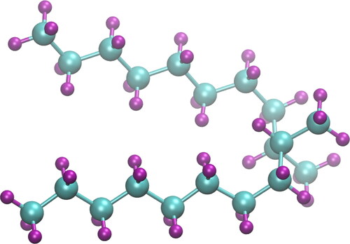As a result, PAO-2 has a kinematic viscosity of about 2 mm²/s (cSt) at 100 ${}^{°}$C and consists mainly of hydrogenated 1-decene dimer isomers (C₂₀H₄₂), from which 9,10-dimethyloctadecane is the most abundant (35) and is chosen for this theoretical study. For comparison with experiment, the PAO-2 sample that was used in this study contained more than 95% of hydrogenated 1-decene dimer by weight (36). The atomic structure of the selected molecule prior to energy relaxation and equilibration can be seen in Figure 1.

Figure 1. Molecular structure of 9,10-dimethyloctadecane, main component of PAO-2. Carbons are shown as cyan spheres and hydrogens as purple spheres. The conformation shown is prior to equilibration and, therefore, has a relatively linear structure.

As there are relatively few studies examining the high pressure rheology of lubricants from a computational point of view, in this study, we examine the very interesting behavior of a lubricant through molecular simulation approaches. We perform bulk NEMD and EMD-GK simulations of viscosity with parameters such as temperature and pressure that have values that can be encountered under operational conditions. This paper aims to showcase the significance of the choice of method for calculating viscosity, by comparing available simulation approaches in order to find which works best when comparing to experimental data. The simulations are performed at different temperatures and pressures (up to 1.0 GPa), while investigating the shear rate dependence of viscosity. We have compared our simulation results with available experimental data of shear viscosity for each condition that was tested.

Methodology

Calculation of zero shear viscosity with equilibrium molecular dynamics

One of the main methods that allow the numerical calculation of zero shear viscosity of a liquid is Green-Kubo equilibrium molecular dynamics (EMD-GK), which is based on the fluctuation-dissipation theorem (37). Green and Kubo proved (4, 5) that the coefficients describing the transport properties of the system (e.g., viscosity) are represented by equilibrium fluctuations of internal properties. These fluctuations can be evaluated by integrals of autocorrelation functions (ACFs) of these internal properties. The zero shear viscosity η is calculated using the formula: [1] $${\eta }_{\alpha \beta }(t)=\frac{V}{k_{\mathrm{B}}T}\underset{0}{\overset{t}{\int }}〈P_{\alpha \beta }(0)P_{\alpha \beta }(t\prime )〉\mathrm{d}t\prime$$[1] where V is the volume of the particle system, T is temperature, $k_{\mathrm{B}}$ is the Boltzmann constant, $〈\dots 〉$ is averaging over the ensemble that uses the three unique off-diagonal pressure tensor elements, namely P_xy, P_yz, P_xz, $\alpha \beta \equiv x,y,z$ and $t\prime$ and t are time. Then the zero shear viscosity is the average of the three viscosity components η_xy, η_yz and η_xz. For practical reasons in simulations, the upper limit of the above integral is set to a certain time, which is sufficiently long to ensure the noise-free decay of the ACF and convergence of viscosity (2). Moreover, EMD-GK is known to work well only for fluids with relatively low viscosity (38), typically less than 20 mPa s, which means that it is difficult to use this approach to compute viscosity at high pressures, where the viscosity of a lubricant is known to increase dramatically.

The instantaneous value of the pressure tensor that is used in Eq. 1[1] $${\eta }_{\alpha \beta }(t)=\frac{V}{k_{\mathrm{B}}T}\underset{0}{\overset{t}{\int }}〈P_{\alpha \beta }(0)P_{\alpha \beta }(t\prime )〉\mathrm{d}t\prime$$[1] and is calculated at each time, is given by the following equation (39): [2] $$P_{\alpha \beta }(t)=\frac{\sum _{i=1}^K{m}_i{u}_{i\alpha }(t)u_{i\beta }(t)}{V}+\frac{\sum _{i=1}^{K\prime }{r}_{i\alpha }(t)f_{i\beta }(t)}{V}$$[2] where P_αβ is the value of the pressure tensor at time t, m_i is mass, $u_{i\alpha }$ and $u_{i\beta }$ are velocities in direction of the α or β dimension of atom i, $r_{i\alpha }$ and $f_{i\beta }$ are the position and force vector components of atom i, with a total of K atoms. Then $K\prime$ extends the sum to include periodic image (ghost) atoms outside of the central simulation box, when periodic boundary conditions are enforced in conjunction with the minimum image convention (40). The use of ghost atoms is required so that all forces can be computed from each atom, within a specified cut-off distance.

Finally, Eq. 1[1] $${\eta }_{\alpha \beta }(t)=\frac{V}{k_{\mathrm{B}}T}\underset{0}{\overset{t}{\int }}〈P_{\alpha \beta }(0)P_{\alpha \beta }(t\prime )〉\mathrm{d}t\prime$$[1] is discretized with simple quadrature (trapezoidal rule) to obtain zero shear viscosity: [3] $${\eta }_{\alpha \beta }(\mathit{\text{kdδt}})=\frac{1}{2}[C_{\alpha \beta ,0}(\mathit{\text{kdδt}})+2\sum _{N=1}^{p-2}{C}_{\alpha \beta ,N}(\mathit{\text{kdδt}})+C_{\alpha \beta ,p-1}(\mathit{\text{kdδt}})]\frac{V}{k_{\mathrm{B}}T}s\delta t$$[3]

The viscosity is converged when it becomes time-independent and this can be checked by performing autocorrelation over an increasing number k of snapshot multiples during the production run, as shown in Eq. 3[3] $${\eta }_{\alpha \beta }(\mathit{\text{kdδt}})=\frac{1}{2}[C_{\alpha \beta ,0}(\mathit{\text{kdδt}})+2\sum _{N=1}^{p-2}{C}_{\alpha \beta ,N}(\mathit{\text{kdδt}})+C_{\alpha \beta ,p-1}(\mathit{\text{kdδt}})]\frac{V}{k_{\mathrm{B}}T}s\delta t$$[3] , with the same time origin (beginning of the production run).

Calculation of shear viscosity with nonequilibrium molecular dynamics

Although viscosity can be obtained by EMD, it is a nonequilibrium property. A method that uses a more intuitive way to understand the definition of viscosity, as shown in Eq. 4[4] $$\eta \left(t\right)=-\frac{P_{xy}(t)}{\dot{\gamma }}$$[4] , is known as nonequilibrium molecular dynamics (NEMD). For example, the SLLOD algorithm (39, 41), which is compatible with Lees-Edwards “sliding-brick” boundary conditions (42) for shear flow of infinite extent, is a very efficient algorithm that sets up a steady planar Couette flow with a velocity profile that is linear across the sample thickness. This allows the calculation of viscosity with a constant shear rate ($\dot{\gamma }$), which is not directly applied to the sample, but is derived from the shear velocity and the sample thickness, as stated in Eq. 5[5] $$\dot{\gamma }=\frac{U_x}{h}$$[5] . 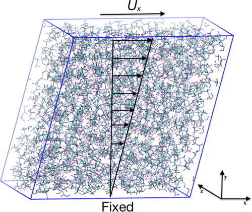In NEMD, in order to capture both Newtonian and shear thinning regions, it is essential to run several simulations with different shear rates, with the time-varying viscosity equal to: [4] $$\eta \left(t\right)=-\frac{P_{xy}(t)}{\dot{\gamma }}$$[4] and [5] $$\dot{\gamma }=\frac{U_x}{h}$$[5] where η is the shear viscosity, P_xy is the value of the pressure tensor in the xy plane, $\dot{\gamma }$ is the shear rate, U_x is the applied velocity at the top edge of the simulation box and h is the sample thickness in the y dimension. The shearing process using the SLLOD algorithm can be seen in Figure 2. The simulation box is sheared along the xy plane and a constant velocity vector is applied at the top edge of the simulation box.

Figure 2. Schematic showing the shearing process with the SLLOD algorithm for Couette flow. A shearing velocity is applied at the top edge of the simulation box, with the algorithm creating a linear velocity profile. Periodic boundary conditions are enforced in all three dimensions. Rendered using VMD (70).

Then Eq. 4[4] $$\eta \left(t\right)=-\frac{P_{xy}(t)}{\dot{\gamma }}$$[4] describes the Newtonian behavior of a fluid, but fluids can also exhibit non-Newtonian behavior, where viscosity depends on the applied shear rate. Various empirical and microscopic models are available (43) to characterize such behavior of fluids out of which, the Powell-Eyring model (44) is chosen for curve fitting of the MD results in the present study, as it has been suggested that viscosity extrapolation schemes can be useful at very high pressures (27–29). The Powell-Eyring model,¹ although more mathematically complex, has certain advantages over other common models as it is based on the kinetic theory of liquids rather than empiricism: [6] $$\eta (\dot{\gamma })=({\eta }_N-{\eta }_{\infty })\frac{{\text{sinh}}^{-1}(\tau \dot{\gamma })}{\tau \dot{\gamma }}+{\eta }_{\infty }$$[6] where ${\eta }_{\infty }$ is shear viscosity at infinite shear rate, η_N is the Newtonian viscosity, $\tau$ is the characteristic relaxation time and ${\text{sinh}}^{-1}$ denotes the inverse hyperbolic sine function. At shear rates higher than the critical shear rate ${\dot{\gamma }}_{\text{cr}}=1/\tau ,$ the fluid transitions from Newtonian to non-Newtonian behavior (shear thinning).

Simulation details

All equilibrium and nonequilibrium molecular dynamics simulations were carried out by using the LAMMPS software (45), combined with some in-house developed scripts to perform autocorrelation and averaging of viscosity. The necessary files, that included the coordinates of molecules, the simulation settings and atomic charges needed for LAMMPS, were generated with Moltemplate (46). Moltemplate is an open-source software that can generate LAMMPS input scripts. The molecular system structures needed in Moltemplate were generated with Packmol (47), which reads simple .xyz file coordinates in order to fill simulation boxes of specified size with molecules that have randomized arrangement. A box with a starting volume of $65.0\times 65.0\times 65.0$ ų, containing 170 9,10-dimethyloctadecane molecules (10,540 atoms) was generated and periodic boundary conditions were applied in all three dimensions. In this work, the L-OPLS-AA and GAFF2-AA force fields were chosen. L-OPLS-AA (48) is a force field specifically optimized for long-chain hydrocarbons while GAFF2-AA is a general-purpose force field (49). The functional form of these force fields is expressed as: [7] $$U({\mathbf{r}}^K)=U_{\text{bond}}+U_{\text{angle}}+U_{\text{dihedral}}+U_{\text{nonbond}}$$[7] where $U_{\text{bond}}$ defines the harmonic vibrational motion between bonded atoms with respect to the equilibrium bond length, $U_{\text{angle}}$ defines the angular vibrational motion of three atoms with respect to the equilibrium bond angle, $U_{\text{dihedral}}$ refers to torsional rotation of four atoms with respect to a central bond and $U_{\text{nonbond}}$ refers to pairwise interactions (Lennard-Jones and electrostatics). All force field coefficients that were used in this work are available in the Supporting Information.

For both force fields, the cut-off radius for Lennard-Jones interactions was fixed at 13.0 Å (2), including a long-range Van der Waals tail correction (50) to the energy and pressure. “Unlike” Lennard-Jones interactions between different atoms (such as C and H) were evaluated using the geometric mean mixing rules (51) for calculating the potential wall depth ϵ_ij and the collision diameter σ_ij of pairwise interactions. For GAFF2-AA, an additional outer cut-off radius needs to be specified and was fixed at 15.0 Å, as it is typical to make the difference between the inner and outer cut-off radius about 2.0 Angstroms.

For L-OPLS-AA, long-range electrostatic interactions were not cut off, but were evaluated using the particle-particle particle-mesh (PPPM) method (52) with a relative force accuracy of 10^–4. This method maps atomic charges to a three-dimensional mesh and uses Finite Fourier Transform to solve Poisson’s equation on the mesh and then interpolates electric fields on the mesh points back to the atoms. In that way, each charge in the system interacts with charges in an infinite array of periodic images of the simulation domain. For GAFF2-AA, short-range electrostatic interactions require a cut-off radius, which was also fixed at 15.0 Å. This means that, within this distance, interactions are computed directly, while interactions outside that distance are computed in conjunction with the PPPM method.

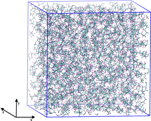
The simulation started with an energy relaxation process, followed by a run of 2 ps in the isoenthalpic-isobaric (NPH) ensemble (53, 54) with a Langevin thermostat (55), in order to allow the molecules to reorient themselves. This is not a necessary step, but it has been suggested that it can speed up density equilibration by randomizing the molecules’ coordinates and we have noticed that other molecules such as cyclohexane, would have a much slower density equilibration if this step is omitted. To equilibrate the density, a run of 20 ns in the isothermal-isobaric (NPT) ensemble followed, with a timestep of 1 fs, and the system’s volume was allowed to vary until it reached equilibrium. To control temperature and pressure, a Nose-Hoover thermostat and barostat (56, 57) were used at the temperature and pressure of choice with a time constant of 0.1 ps and 1 ps, respectively. This was followed by a 2 ns run in the canonical (NVT) ensemble with a Nose-Hoover thermostat. For 9,10-dimethyloctadecane, density equilibration took place at four selected temperatures, at 313, 343, 373 and 423 K (40, 70, 100 and 150 ${}^{°}$C respectively), with pressure ranging from 0.1 MPa to 1.0 GPa (11 data points in total). Figure 3 shows a snapshot of this simulation with 9,10-dimethyloctadecane molecules after density equilibration. Carbon atoms are colored with cyan and hydrogen atoms with purple. Periodic boundary conditions are enforced in all directions. At that point, after equilibration in the NPT ensemble, the density had an average fluctuation of ± 0.005 g/mL (standard deviation, last 5 ns), which is a negligible difference of ± 0.6% and thus the system can be said to be stable.

Figure 3. Equilibrated system of 9,10-dimethyloctadecane at 40 ${}^{°}$C and 0.1 MPa using the L-OPLS-AA force field.

The zero shear viscosity (EMD-GK) was then calculated with the following procedure. The final state of the previous simulation, with a volume cell of equilibrated molecules, was used as the initial configuration (equilibrated density). To improve statistics, five independent trajectories were then produced by randomizing the initial configuration. This was achieved by heating and then cooling the initial configuration through separate cycles and then the pressure tensor was collected for each run. These heat-quench cycles (2) for simulations at 313 K were performed from 313 K to T = 315, 320, 325, 330, and 335 K, respectively, during 1 ns runs in the NVT ensemble, after which the systems were immediately quenched back to 313 K during another 1 ns run in the NVT ensemble. Simulations at 373 K included heat-quench cycles that were from 373 K to T = 375, 380, 385, 390 K, and 395 K, respectively, during 1 ns runs in the NVT ensemble, after which the systems were immediately quenched back to 373 K during another 1 ns run in the NVT ensemble. Then the systems ran in the NVT ensemble for another 40 ns and the viscosity was calculated by the running average integral of the autocorrelation function of the pressure tensor in three dimensions as specified in the Green-Kubo method in Eq. 3[3] $${\eta }_{\alpha \beta }(\mathit{\text{kdδt}})=\frac{1}{2}[C_{\alpha \beta ,0}(\mathit{\text{kdδt}})+2\sum _{N=1}^{p-2}{C}_{\alpha \beta ,N}(\mathit{\text{kdδt}})+C_{\alpha \beta ,p-1}(\mathit{\text{kdδt}})]\frac{V}{k_{\mathrm{B}}T}s\delta t$$[3] . The parameters that were used for autocorrelation were a sampling rate of s = 5 fs, with a number of autocorrelation terms p = 100,000 over a time period of d = $s p$ = 0.5 ns.

The nonequilibrium shear viscosity was calculated with the following procedure for the four selected temperatures. Starting again from the state of equilibrated density (after a 20 ns run in the NPT ensemble), five independent trajectories were produced by separate heat-quench cycles, as described in the previous paragraph (313 and 373 K case). For the remaining two temperatures (343 and 423 K case), the heat-quench cycles were the following. Simulations at 343 K included heat-quench cycles that were from 343 K to T = 345, 350, 355, 360 K, and 365 K, respectively, during 1 ns runs in the NVT ensemble, after which the systems were immediately quenched back to 343 K during another 1 ns run in the NVT ensemble. Simulations at 423 K included heat-quench cycles that were from 423 K to T = 425, 430, 435, 440 K, and 445 K, respectively, during 1 ns runs in the NVT ensemble, after which the systems were immediately quenched back to 423 K during another 1 ns run in the NVT ensemble. The simulation settings were the same as the EMD case (zero shear). 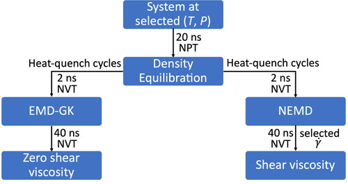Then for five different values of applied shear rate (from ${10}^{6.5}$ up to ${10}^{8.5}$ s⁻¹), the SLLOD algorithm was used and the simulation box was deformed across the xy plane, achieving simple Couette flow. The system was then sheared for 20 ns to ensure a steady state, followed by a production run of 40 ns, and the nonequilibrium viscosity was calculated for each shear rate and trajectory. The whole simulation ran in the NVT ensemble with a Nose-Hoover thermostat and a time constant of 0.01 ps. The same procedure was repeated for all different pressure values. A diagram that summarizes the whole simulation process is presented in Figure 4.

Figure 4. Diagram summarizing the steps of the simulation for calculating viscosity with EMD-GK and NEMD.

Experimental procedure for measuring viscosity at high pressures for PAO-2

The viscosity of PAO-2 (Spectrasyn 2 from ExxonMobil) was characterized in a falling cylinder viscometer (58). The sinkers apply shear stress of less than 100 Pa so that the viscosity may be considered the limiting low shear value. Two viscometers, each employing two different sinkers, were used and the results were averaged. The uncertainty in temperature is 0.5 ${}^{°}$C, 3 MPa in pressure and 3% in viscosity. The usual inflection in the pressure versus log viscosity curve is not present in this oil to 1.0 GPa at the temperatures investigated.

Results and discussion

The pressure–density response of hydrocarbons is commonly described using the Tait equation (59): [8] $$\frac{\rho (P)-{\rho }_0}{\rho (P)}=C{\hspace{0.17em}\text{log}\hspace{0.17em}}_{10}\left(\frac{B+P}{B+P_0}\right)$$[8] where C and B are fitted parameters, ρ is the density at pressure P and ρ₀ is the density at ambient pressure P₀. The parameters that were used for the fits to the Tait equation in Figure 5 are given in Table 1. For all of the force field and conditions studied, the Tait equation provided an excellent estimation of the density acquired from the MD simulations (average density, last 5 ns), as demonstrated by the low root-mean square error (RMSE).

Figure 5. The dependence of density on pressure for 9,10-dimethyloctadecane at 40, 70, 100 and 150 ${}^{°}$C. Circles indicate density results by using the L-OPLS-AA force field, while squares indicate results acquired with the GAFF2-AA force field. The dashed lines indicate Tait fits (eq. 8[8] $$\frac{\rho (P)-{\rho }_0}{\rho (P)}=C{\hspace{0.17em}\text{log}\hspace{0.17em}}_{10}\left(\frac{B+P}{B+P_0}\right)$$[8] ) to the MD simulation data. The parameters that were used for the fits are given in Table 1.

Table 1. Parameters with the RMSE used in the Tait fits (Eq. 8[8] $$\frac{\rho (P)-{\rho }_0}{\rho (P)}=C{\hspace{0.17em}\text{log}\hspace{0.17em}}_{10}\left(\frac{B+P}{B+P_0}\right)$$[8] ) for the MD data in Figure 5. The root-mean square errors are between simulation data and the Tait approximations. Note that P₀ is equal to 0.1 MPa.

Force field	${\mathit{\rho }}_{\mathbf{0}}$ (g/ml)	C	B (MPa)	RMSE (g/ml)	T (${}^{°}$C)
L-OPLS-AA	0.780 ± 0.005	0.1864	93.0	0.0003	40
GAFF2-AA	0.790 ± 0.004	0.1786	121.9	0.0004	40
L-OPLS-AA	0.756 ± 0.005	0.1912	79.5	0.0003	70
L-OPLS-AA	0.733 ± 0.005	0.1959	67.2	0.0003	100
L-OPLS-AA	0.695 ± 0.007	0.1991	49.5	0.0002	150

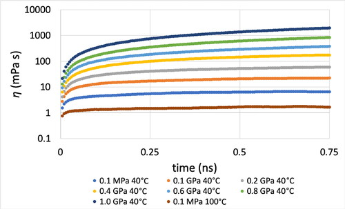
The choice of t for the upper limit of the EMD-GK integral (Eq. 1[1] $${\eta }_{\alpha \beta }(t)=\frac{V}{k_{\mathrm{B}}T}\underset{0}{\overset{t}{\int }}〈P_{\alpha \beta }(0)P_{\alpha \beta }(t\prime )〉\mathrm{d}t\prime$$[1] ) cannot be known a priori as it depends on the selected molecule and conditions such as temperature and pressure. For this reason, it was determined by using various d time values of autocorrelation until the viscosity estimate for a given simulation replicate converges (Figure 6). This behavior shows that the autocorrelation function of the pressure tensor has successfully decayed to zero. As can be seen from the graph, performing autocorrelation for 0.5 ns, with sufficient data points of the pressure tensor, results in an accurate estimate within the region of applicability of EMD-GK. It is found that the EMD-GK method is applicable to pressures up to 0.3 GPa, as at higher pressures, the method has issues with the decay of the autocorrelation function of the pressure tensor (highly viscous systems).

Figure 6. Convergence of viscosity for various d time values of autocorrelation for 9,10-dimethyloctadecane at 40 ${}^{°}$C and pressures from 0.1 MPa to 1.0 GPa and 100 ${}^{°}$C at 0.1 MPa. The pressure tensor values are used every s = 5 fs during the production run of 40 ns.

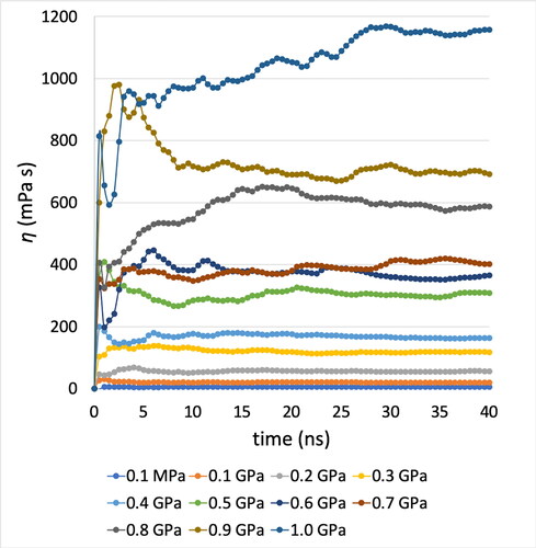
The ratio between the dynamic (low shear) viscosity and the density of a fluid is equal to the kinematic viscosity. By using the L-OPLS-AA force field, the simulated (zero shear rate, EMD method) kinematic viscosity of 9,10-dimethyloctadecane at 100 °C and 0.1 MPa was equal to 2.0 ± 0.3 mm²/s, which is in close agreement with the experimental value of 1.8 mm²/s (60), as it was overestimated by just 14%. The kinematic viscosity at 40 °C was found to be 6.8 ± 0.8 mm²/s, which yields an overestimation of 28% when compared with the experimental value of 5.3 mm²/s (60). Then the running integral (equal to the zero shear viscosity) of the autocorrelation function of the pressure tensor at 40 °C and pressures from 0.1 MPa to 1.0 GPa for 9,10-dimethyloctadecane, can be seen in Figure 7. It is necessary that simulations run for long enough so that the viscosity result converges.

Figure 7. Convergence of viscosity with time. Running EMD-GK integral of 9,10-dimethyloctadecane zero shear viscosity at 40 ${}^{°}$C and pressures from 0.1 MPa to 1.0 GPa using the L-OPLS-AA force field. Five trajectories are used to calculate the average value and the autocorrelation is performed by using the pressure tensor every s = 5 fs with a total number of p = 100,000 autocorrelation terms.

For the NEMD case, viscosity was acquired successfully for pressures up to 1.0 GPa and the applied shear rates varied from 10^6.5 up to ${10}^{8.5}$ s⁻¹. The selected shear rates in this work can be directly linked to the accessible shear rates in tribological experiments of rolling-sliding contact, where the shear rate is typically 10⁵ to 10⁷ s⁻¹ (61), while high-performance engine components can extend up to 10⁸ s⁻¹ (62). Figure 8 shows the viscosity obtained from the simulations as a function of the applied shear rate over the pressure range of 0.1 MPa to 1.0 GPa at 40 °C, illustrating how the critical shear rate (onset of shear thinning (63), which has been similarly observed for an ionic liquid (64)) changes with pressure. For example, at 0.8 GPa (with L-OPLS-AA), shear thinning behavior was observed at higher shear rates ($\dot{\gamma }$ > 10⁷ s⁻¹) and the Newtonian regime was captured at $\dot{\gamma }$ < 10⁷ s⁻¹. It was found that the simulated low shear viscosity, which was calculated with Eq. 4[4] $$\eta \left(t\right)=-\frac{P_{xy}(t)}{\dot{\gamma }}$$[4] , was very close with the experimental value at the specified pressure, but simulation data were also fitted to Powell-Eyring equation (black dashed line, Eq. 6[6] $$\eta (\dot{\gamma })=({\eta }_N-{\eta }_{\infty })\frac{{\text{sinh}}^{-1}(\tau \dot{\gamma })}{\tau \dot{\gamma }}+{\eta }_{\infty }$$[6] ) and zero shear viscosity was acquired with zero shear rate extrapolation. For pressures up to 0.7 GPa, the simulated shear rates were low enough to reach the Newtonian regime at shear rates ($\dot{\gamma }$) ranging from 10⁷ s⁻¹ up to ${10}^{8.5}$ s⁻¹. For these pressures, viscosity was obtained directly from an average over points in the Newtonian plateau, a procedure that has been also used in similar studies (27, 28). For the remaining high pressure NEMD simulations (up to 1.0 GPa), viscosity was obtained by zero shear rate extrapolation of Powell-Eyring fits (Eq. 6[6] $$\eta (\dot{\gamma })=({\eta }_N-{\eta }_{\infty })\frac{{\text{sinh}}^{-1}(\tau \dot{\gamma })}{\tau \dot{\gamma }}+{\eta }_{\infty }$$[6] ) to simulation data. The parameters that were used for the fits to the Powell-Eyring equation in Figure 8 (40 °C case) and the other three tested temperatures are given in Table 2. The Powell-Eyring equation fitted very well the high pressure viscosity data acquired from MD simulations, as demonstrated by the low root-mean square error (RMSE). Another observation was that the standard deviation of the NEMD viscosity results increases as shear rate decreases. For example, at 0.4 GPa and 40 °C the standard deviation of viscosity (five independent trajectories) with L-OPLS-AA at shear rates of 10⁸, ${10}^{7.5}$ and 10⁷ s⁻¹ was equal to ± 5.1, ± 37.1 and ± 76.7 mPa s, respectively. This is a typical behavior in NEMD simulations as at lower shear rates, the systematic nonequilibrium response becomes comparable to the equilibrium fluctuations. This leads to a lower signal-to-noise ratio and an increase of viscosity variability (3).

Figure 8. NEMD shear viscosity of 9,10-dimethyloctadecane (PAO-2) at 40 ${}^{°}$C and pressures from 0.1 MPa to 1.0 GPa. Experimental data were acquired by averaging viscosity measurements from two different viscometers. One of the viscosity data sets used in the averaging has been previously published (69). Each simulation data point represents the average viscosity value of five independent simulations, at each shear rate. Circles indicate viscosity results by using the L-OPLS-AA force field, while triangles indicate results acquired with the GAFF2-AA force field. Squares indicate experimental viscosity values. Horizontal solid lines indicate the average viscosity obtained for pressures where the applied shear rates had reached the Newtonian regime. The dashed lines indicate Powell-Eyring fits (Eq. 6[6] $$\eta (\dot{\gamma })=({\eta }_N-{\eta }_{\infty })\frac{{\text{sinh}}^{-1}(\tau \dot{\gamma })}{\tau \dot{\gamma }}+{\eta }_{\infty }$$[6] ) to MD simulation data that extrapolate to zero shear rate (Newtonian limit). The black dashed line corresponds to the L-OPLS-AA force field and the red dashed line corresponds to the GAFF2-AA force field. The parameters that were used for the fits are given in Table 2.

Table 2. Parameters with the root-mean square error (RMSE) used in the Powell-Eyring fits (Eq. 6[6] $$\eta (\dot{\gamma })=({\eta }_N-{\eta }_{\infty })\frac{{\text{sinh}}^{-1}(\tau \dot{\gamma })}{\tau \dot{\gamma }}+{\eta }_{\infty }$$[6] ) for the MD data in Figure 8 (40 °C case) and the other three tested temperatures. The root-mean square errors are between simulation data and the Powell-Eyring approximations.

Force Field	P (GPa)	${\mathit{\eta }}_{\mathit{N}}$ (Pa s)	$\mathit{\tau }$ (s)	${\mathit{\eta }}_{\infty }$ (Pa s)	RMSE (Pa s)	T (${}^{°}$C)
L-OPLS-AA	0.8	4.99	1.74 $\times {10}^{-7}$	0	0.10	40
L-OPLS-AA	0.9	9.36	2.63 $\times {10}^{-7}$	0	0.14	40
L-OPLS-AA	1.0	12.59	3.61 $\times {10}^{-7}$	0	0.14	40
GAFF2-AA	0.8	10.46	3.35 $\times {10}^{-7}$	0	0.21	40
GAFF2-AA	1.0	15.71	5.01 $\times {10}^{-7}$	0	0.12	40
L-OPLS-AA	0.8	1.94	8.77 $\times {10}^{-8}$	0	0.04	70
L-OPLS-AA	0.9	3.58	1.38 $\times {10}^{-7}$	0	0.04	70
L-OPLS-AA	1.0	4.09	1.42 $\times {10}^{-7}$	0	0.09	70
L-OPLS-AA	0.8	0.61	3.58 $\times {10}^{-8}$	0	0.001	100
L-OPLS-AA	0.9	1.05	5.21 $\times {10}^{-8}$	0	0.01	100
L-OPLS-AA	1.0	1.80	6.97 $\times {10}^{-8}$	0	0.05	100
L-OPLS-AA	0.8	0.12	6.67 $\times {10}^{-9}$	0	0.01	150
L-OPLS-AA	0.9	0.17	9.36 $\times {10}^{-9}$	0	0.01	150
L-OPLS-AA	1.0	0.26	1.47 $\times {10}^{-8}$	0.01	0.01	150

Figure 9 shows the zero shear viscosity-pressure relation of 9,10-dimethyloctadecane, in which we are comparing two methods (EMD and NEMD) and two force fields (L-OPLS-AA and GAFF2-AA) with experimental data for the pressure range of 0.1 MPa up to 1.0 GPa at 40 °C, where viscosity has a huge variation. For EMD simulations, we observed good agreement for viscosity values up to 0.3 GPa. Simulations started to diverge from experiment at higher pressures where EMD is no longer suitable, due to the exponential increase of viscosity and the very long rotational relaxation times of the less flexible molecules of larger size (65). The rotational relaxation time refers to the required time for molecular chains to reach equilibrium after an external perturbation. In the Green-Kubo method, errors accumulate at long times and, as a result, this is not something that can be remedied simply by using longer trajectories (65). The time decomposition method (12) may help to some degree, as recently demonstrated for 2,2,4-trimethylhexane up to viscosities of 20 mPa s (66) and for a binary mixture of methylcyclohexane and 1-methylnaphthalene up to viscosities of 50 mPa s (20). However, at higher viscosites, NEMD with extrapolation back to the Newtonian viscosity (using the Eyring equation) seems to be the only reliable method (this study and (27–29)). An important observation is that the region where EMD fails to predict the exponential increase of viscosity (compared to the experiment at P > 0.3 GPa) in this study, corresponds to literature suggestions (38) that NEMD is preferable to EMD for viscosity calculations of high-viscosity materials (above 20-50 mPa s). On the other hand, NEMD simulations performed much better and were able to capture high pressure viscosity successfully, although they tended to slightly overestimate viscosity at low pressures, where EMD performed slightly better. As can also be seen from the graph, the L-OPLS-AA force field was more accurate than the GAFF2-AA force field, with the L-OPLS-AA force field overestimating viscosity by only 2% at a pressure of 0.8 GPa. This could be due to the fact that GAFF2-AA is a general-purpose force field, while L-OPLS-AA is specifically designed for long-chain hydrocarbons. Figure 10 shows the effect of temperature on the viscosity-pressure relation of 9,10-dimethyloctadecane, in which we are comparing viscosity results acquired from NEMD simulations (using the L-OPLS-AA force field) and experimental data for the pressure range of 0.1 MPa up to 1.0 GPa. The general tendency is that viscosity is slightly overestimated by NEMD simulations; nonetheless, simulations successfully capture the pressure-viscosity slope, which is equal to the reciprocal asymptotic isoviscous pressure coefficient. We need to note that the experimental PAO-2 sample was not pure 9,10-dimethyloctadecane as used in the simulations, though it contained more than 95% of hydrogenated 1-decene dimer by weight (36). This may be a source of some of the deviations between simulations and experiment.

Figure 9. Zero shear viscosity simulation of 9,10-dimethyloctadecane (PAO-2) at 40 ${}^{°}$C, with pressures ranging from 0.1 MPa to 1.0 GPa. Experimental data were acquired by averaging viscosity measurements from two different viscometers. One of the viscosity data sets used in the averaging has been previously published (69) and experimental data are also provided by (60). Squares indicate experimental viscosity values and circles indicate viscosity results from MD simulations. Statistical error bars are shown when they are larger than the symbol size. For $P\le 0.7,$ GPa simulations reached the Newtonian limit without extrapolation, while, for $P\ge 0.8$ GPa, zero shear viscosity was extrapolated by Powell-Eyring fits (Eq. 6[6] $$\eta (\dot{\gamma })=({\eta }_N-{\eta }_{\infty })\frac{{\text{sinh}}^{-1}(\tau \dot{\gamma })}{\tau \dot{\gamma }}+{\eta }_{\infty }$$[6] ) to simulation data. The dashed lines indicate McEwen fits (Eq. 9[9] $$\eta (P)={\eta }_0{(1+\frac{{\alpha }^{*}P}{q-1})}^q$$[9] ) to the experimental and MD simulation data. The parameters that were used for the fits are given in Table 3.

Figure 10. Zero shear viscosity simulation of 9,10-dimethyloctadecane (PAO-2) at 40, 70, 100 and 150 ${}^{°}$C, with pressures ranging from 0.1 MPa to 1.0 GPa. Squares indicate experimental viscosity values that were acquired by averaging viscosity measurements from two different viscometers. Circles indicate viscosity results by using the L-OPLS-AA force field. Statistical error bars are shown when they are larger than the symbol size. For $P\le 0.7$ GPa, simulations reached the Newtonian limit without extrapolation, while, for $P\ge 0.8$ GPa, zero shear viscosity was extrapolated by Powell-Eyring fits (Eq. 6[6] $$\eta (\dot{\gamma })=({\eta }_N-{\eta }_{\infty })\frac{{\text{sinh}}^{-1}(\tau \dot{\gamma })}{\tau \dot{\gamma }}+{\eta }_{\infty }$$[6] ) to simulation data. The dashed lines indicate McEwen fits (Eq. 9[9] $$\eta (P)={\eta }_0{(1+\frac{{\alpha }^{*}P}{q-1})}^q$$[9] ) to the experimental and MD simulation data. The parameters that were used for the fits are given in Table 3.

The pressure-viscosity response of lubricants is commonly represented using the McEwen equation (67): [9] $$\eta (P)={\eta }_0{(1+\frac{{\alpha }^{*}P}{q-1})}^q$$[9] where η₀ is the low-shear viscosity at reference (ambient) pressure, ${\alpha }^{*}$ is the reciprocal asymptotic isoviscous pressure coefficient and q is the McEwen exponent. This is equivalent to the Tait pressure-viscosity equation (68) for low (ambient (69)) reference pressures. The parameters that were used for the fits to the McEwen equation in Figure 9 and 10 are given in Table 3. In their region of applicability, which was up to 0.3 GPa for EMD-GK and up to 1.0 GPa for NEMD, the values of ${\alpha }^{*}$ for both EMD-GK and NEMD methods were in reasonable agreement with experiment when the L-OPLS-AA force field was used. For example, at 40 ${}^{°}$C the value of ${\alpha }^{*}$ was overestimated by 15% with NEMD and by only 3% with EMD-GK when comparing to experiment. At higher temperatures (100 and 150 ${}^{°}$C), NEMD was in good agreement with experiment as the overestimation was only 7% and 6%, respectively. At the medium temperature of 70 ${}^{°}$C, NEMD overestimated the value of ${\alpha }^{*}$ by 44%.

Table 3. Parameters with the root-mean square error (RMSE) used in the McEwen fits (Eq. 9[9] $$\eta (P)={\eta }_0{(1+\frac{{\alpha }^{*}P}{q-1})}^q$$[9] ) for the MD and experimental data in Figure 9 and 10. The root-mean square errors are between simulation/experimental data and the McEwen approximations.

Method	${\mathit{\eta }}_{\mathbf{0}}$ (mPa s)	${\mathit{\alpha }}^{\mathbf{*}}$ (GPa^–1)	q	RMSE (mPa s)	T (${}^{°}$C)
Exp.	3.80	11.49	10.95	11.10	40
NEMD L-OPLS-AA	7.38	13.17	5.38	334	40
NEMD GAFF2-AA	15.21	19.31	2.87	713	40
EMD-GK L-OPLS-AA	5.32	11.88	3.39	0.85	40
Exp.	1.98	9.70	8.56	6.94	70
NEMD L-OPLS-AA	2.99	13.95	4.60	222	70
Exp.	1.20	8.83	6.19	0.40	100
NEMD L-OPLS-AA	1.51	9.45	9.33	13.95	100
Exp.	0.66	7.26	2.43	0.04	150
NEMD L-OPLS-AA	1.03	7.71	5.62	7.38	150

To give an estimate of the computational cost of this work, considering the case of 0.5 GPa at 40 ${}^{°}$C and an applied shear rate of 10⁸ s⁻¹ (for the NEMD case), the following results are representative. The density equilibration and viscosity calculation with EMD-GK (62 ns simulation time in total) required 6117 Core Hours (CPU-h) for one independent trajectory. On the other side, the density equilibration and viscosity calculation with NEMD (82 ns simulation time in total) required 7938 Core Hours (CPU-h) for one independent trajectory.

Conclusions

Molecular dynamics (MD) simulations can be used to compute macroscopic properties of industrial lubricant components from their behavior at the molecular level. In this study, we have performed a critical evaluation of the use of MD to compute the zero shear viscosity of a widely used lubricant such as 9,10-dimethyloctadecane, main component of PAO-2 base oil. We have used and compared the two main techniques for such calculations: the Green-Kubo theory of fluctuations from equilibrium MD (EMD) and the direct computation of viscosity from shear during nonequilibrium MD (NEMD). Our simulations were performed at four different temperatures (40, 70, 100 and 150 °C) and a range of pressures from 0.1 MPa (ambient pressure) up to 1.0 GPa.

We found that EMD simulations, which represent zero shear conditions, were accurate at predicting viscosity values (zero shear) up to 0.3 GPa at 40 ${}^{°}$C. But at higher pressures, where the viscosity increases by three orders of magnitude, EMD became unreliable. This matches observations of other authors (38) that EMD simulations are known to have a limited regime of applicability and should be used for liquids that have relatively low viscosity. High relaxation times, due to high pressures and viscosities, hinder the decay of the ACF and thus, EMD simulations cannot capture viscosity accurately. This means that the upper limit of the integral of the ACF should be chosen to be long enough to ensure convergence of the viscosity by exceeding the rotational relaxation time of the molecule.

On the other hand, NEMD simulations at high pressures successfully captured zero shear viscosity, which was validated against experimental values. As a result, NEMD is suggested to be the method of choice in these operational conditions. We conclude that NEMD can be used to obtain atomic-level insights of lubricant interactions, while providing a reliable approach for computing viscosity, especially in cases where experimental measurement can be difficult.

The choice of force field was also investigated in our study by using two force fields that are similar from a functional point of view but have different parameterization, the L-OPLS-AA and the GAFF2-AA force fields. We found that the L-OPLS-AA force field, which is specifically designed for long-chain hydrocarbons, achieves markedly better agreement with experimental viscosity values than GAFF2-AA, as the L-OPLS-AA force field overestimated viscosity by only 2% at a pressure of 0.8 GPa (40 ${}^{°}$C case) while GAFF2-AA was over by a dramatic 114%. Running simulations either for longer time periods or multiple repeats allowed us to obtain results with an improved confidence interval for viscosity, which was more noticeable at lower shear rates ($\dot{\gamma }$ < 10⁷ s⁻¹) and pressures (P < 0.5 GPa) with NEMD simulations. We also found that, in their region of applicability, the values of the reciprocal asymptotic isoviscous pressure coefficient for both EMD-GK and NEMD methods were in reasonable agreement with experiment when the L-OPLS-AA force field was used. By choosing this force field, we expect that the methods used in this study can be applied to similar lubricants at various temperatures and pressures.

We hope that this study will serve as a benchmark for future simulations of viscosity of lubricants with applications in industry. Our work is applicable in providing practical demonstrations of state-of-the-art simulation of viscosity at high or low values in the Newtonian regime and away from it as well.

Nomenclature
B	=	Fitted parameter, Tait equation
C	=	Fitted parameter, Tait equation
Cαβ	=	Autocorrelation term
d	=	Autocorrelation time interval
$f_{i\beta }$	=	Force vector component
h	=	Sample thickness
k	=	Integer counter of time interval
$k_{\mathrm{B}}$	=	Boltzmann constant
K	=	Number of atoms
$K\prime$	=	Number or ghost atoms
m	=	Mass
N	=	Integer counter of simulation time step
p	=	Number of autocorrelation terms
P	=	Pressure
P0	=	Ambient pressure
Pαβ	=	Pressure tensor
q	=	McEwen exponent
$r_{i\alpha }$	=	Position vector component
S	=	Sampling rate
t	=	Time
T	=	Temperature
$u_{i\alpha }$	=	Velocity vector component
Ux	=	Velocity at the top edge of the simulation box
U	=	Potential energy
$U_{\text{angle}}$	=	Potential energy angle interaction component
$U_{\text{bond}}$	=	Potential energy bonded interaction component
$U_{\text{dihedral}}$	=	Potential energy dihedral interaction component
$U_{\text{nonbond}}$	=	Potential energy non-bonded interaction component
V	=	Volume
${\alpha }^{*}$	=	Reciprocal asymptotic isoviscuous pressure coefficient
$\dot{\gamma }$	=	Shear rate
${\dot{\gamma }}_{\text{cr}}$	=	Critical shear rate
δt	=	Timestep
ϵij	=	Potential wall depth
${\eta }_{\alpha \beta }$	=	Zero shear viscosity component
η0	=	Shear viscosity at reference (ambient) pressure
ηN	=	Newtonian viscosity
${\eta }_{\infty }$	=	Shear viscosity at infinite shear rate
Ρ	=	Density
ρ0	=	Density at ambient pressure
σij	=	Collision diameter
τ	=	Relaxation time

Funding

D.M. acknowledges the funding support of Schaeffler Technologies AG & Co. KG and an EPSRC Doctoral Training Centre Grant (EP/L015382/1) for his Ph.D. studentship. The authors also acknowledge the use of the IRIDIS High Performance Computing Facility (IRIDIS 5) at the University of Southampton. We are grateful to the UK Materials and Molecular Modeling Hub for computational resources, which is partially funded by EPSRC (EP/P020194/1 and EP/T022213/1).

Notes

1 The use of this model in an Elastohydrodynamic Lubrication (EHL) friction calculation results in exaggeration of the thermoviscous regime. The thermal softening response is overstated at high sliding velocity.

References

- Cui, S. T., Cummings, P. T., and Cochran, H. D. (1998), “The Calculation of Viscosity of Liquid n-Decane and n-Hexadecane by the Green-Kubo Method,” Molecular Physics, 93(1), pp 117–122. doi:https://doi.org/10.1080/00268979809482195
- Ewen, J. P., Gattinoni, C., Thakkar, F. M., Morgan, N., Spikes, H. A., and Dini, D. (2016), “A Comparison of Classical Force-Fields for Molecular Dynamics Simulations of Lubricants,” Materials, 9(8), p 651. doi:https://doi.org/10.3390/ma9080651
- Ewen, J. P., Heyes, D. M., and Dini, D. (2018), “Advances in Nonequilibrium Molecular Dynamics Simulations of Lubricants and Additives,” Friction, 6(4), pp 349–386. doi:https://doi.org/10.1007/s40544-018-0207-9
- Green, M. S. (1954), “Random Processes and the Statistical mechanics of time-dependent phenomena. II. irreversible processes in fluids,” J. Chem. Phys., 22(3), pp 398–413. doi:https://doi.org/10.1063/1.1740082
- Kubo, R. (1957), “Statistical-Mechanical Theory of Irreversible Processes. I. General Theory and Simple Applications to Magnetic and Conduction Problems,” Journal of the Physical Society Japan, 12(6), pp 570–586. doi:https://doi.org/10.1143/JPSJ.12.570
- Payal, R. S., Balasubramanian, S., Rudra, I., Tandon, K., Mahlke, I., Doyle, D., and Cracknell, R. (2012), “Shear Viscosity of Linear Alkanes Through Molecular Simulations: Quantitative Tests for n-Decane and n-Hexadecane,” Molecular Simulation, 38(14–15), pp 1234–1241.
- Kirova, E. M., and Norman, G. E. (2015), “Viscosity Calculations at Molecular Dynamics Simulations,” Journal of Physics: Conference Series, 653, 012106. doi:https://doi.org/10.1088/1742-6596/653/1/012106
- Hoover, W. G., Evans, D. J., Hickman, R. B., Ladd, A. J. C., Ashurst, W. T., and Moran, B., (1980), “Lennard-Jones Triple-Point Bulk and Shear Viscosities. Green-Kubo theory, Hamiltonian Mechanics, and Nonequilibrium Molecular Dynamics,” Physical Review A, 22(4), pp 1690–1697. doi:https://doi.org/10.1103/PhysRevA.22.1690
- Ryckaert, J.-P., Bellemans, A., Ciccotti, G., and Paolini, G. V., (1989), “Evaluation of Transport Coefficients of Simple Fluids by Molecular Dynamics: Comparison of Green-Kubo and Nonequilibrium Approaches for Shear Viscosity,” Physical Review A, 39(1), pp 259–267.
- Ramasamy, U. S., Len, M., and Martini, A., (2017), “Correlating Molecular Structure to the Behavior of Linear Styrene-Butadiene Viscosity Modifiers,” Tribology Letters, 65(4), p 147.
- Jones, R. E., and Mandadapu, K. K., (2012), “Adaptive Green-Kubo Estimates of Transport Coefficients from Molecular Dynamics Based on Robust Error Analysis,” Journal of Chemical Physics, 136(15), p 154102. doi:https://doi.org/10.1063/1.3700344
- Zhang, Y., Otani, A., and Maginn, E. J. (2015), “Reliable Viscosity Calculation from Equilibrium Molecular Dynamics Simulations: A Time Decomposition Method,” Journal of Chemical Theory and Computation, 11(8), pp 3537–3546.
- Feng, Y., Goree, J., Liu, B., and Cohen, E. G. D. (2011), “Green-Kubo Relation for Viscosity Tested Using Experimental Data for a Two-Dimensional Dusty Plasma,” Physical Review E, Statistical, Nonlinear, and Soft Matter Physics, 84(4 Pt 2), p 046412. doi:https://doi.org/10.1103/PhysRevE.84.046412
- Wesp, C., El, A., Reining, F., Xu, Z., Bouras, I., and Greiner, C. (2011), “Calculation of Shear Viscosity Using Green-Kubo Relations within a Parton Cascade,” Physical Review C, 84(5), p 054911. doi:https://doi.org/10.1103/PhysRevC.84.054911
- Matsuoka, H., (2012), “Green-Kubo Formulas with Symmetrized Correlation Functions for Quantum Systems in Steady States: The Shear Viscosity of a Fluid in a Steady Shear Flow,” Journal of Statistical Physics, 148(5), pp 933–950.
- Moore, J. D., Cui, S. T., Cochran, G. D., and Cummings, P. T. (2000), “Rheology of Lubricant Basestocks: A Molecular Dynamics Study of C30 Isomers,” Journal of Chemical Physics, 113(19), pp 8833–8840.
- Van-Oanh, N.-T., Houriez, C., and Rousseau, B. (2010), “Viscosity of the 1-Ethyl-3-Methylimidazolium bis(trifluoromethylsulfonyl)imide Ionic Liquid from Equilibrium and Nonequilibrium Molecular Dynamics,” Physical Chemistry Chemical Physics, 12(4), pp 930–936. doi:https://doi.org/10.1039/b918191a
- Mouas, M., Gasser, J.-G., Hellal, S., Grosdidier, B., Makradi, A., and Belouettar, S. (2012), “Diffusion and Viscosity of Liquid Tin: Green-Kubo Relationship-Based Calculations from Molecular Dynamics Simulations’” Journal of Chemical Physics, 136(9), p 094501.
- Kirova, E. M., and Pisarev, V. V. (2016). “Study of Viscosity of Aluminum Melt During Glass Transition by Molecular Dynamics and Green-Kubo Formula,” Journal of Physics: Conference Series, 774, p 012032. doi:https://doi.org/10.1088/1742-6596/774/1/012032
- Kondratyuk, N. D., Pisarev, V. V., and Ewen, J. P. (2020), “Probing the High-Pressure Viscosity of Hydrocarbon Mixtures Using Molecular Dynamics Simulations” Journal of Chemical Physics, 153(15), p 154502. doi:https://doi.org/10.1063/5.0028393
- Liu, P., Lu, J., Yu, H., Ren, N., Lockwood, F. E., and Wang, Q. J. (2017), “Lubricant Shear Thinning Behavior Correlated with Variation of Radius of Gyration Via Molecular Dynamics Simulations,” Journal of Chemical Physics, 147(8), p 084904. doi:https://doi.org/10.1063/1.4986552
- Ewen, J. P., Gao, H., Müser, M. H., and Dini, D. (2019), “Shear heating, flow, and friction of confined molecular fluids at high pressure,” Physical Chemistry Chemical Physics, 21, pp 5813–5823. doi:https://doi.org/10.1039/c8cp07436d
- Prentice, I. J., Liu, X., Nerushev, O. A., Balakrishnan, S., Pulham, C. R., and Camp, P. J. (2020), “Experimental and Simulation Study of the High-Pressure Behavior of Squalane and Poly-α-Olefins,” Journal of Chemical Physics, 152(7), p 074504. doi:https://doi.org/10.1063/1.5139723
- Moore, J. D., Cui, S. T., Cummings, P. T., and Cochran, H. D. (1997), “Lubricant Characterization by Molecular Simulation,” AIChE Journal, 43(12), pp 3260–3263. doi:https://doi.org/10.1002/aic.690431215
- Yang, Y., Pakkanen, T. A., and Rowley, R. L. (2002), “NEMD Simulations of Viscosity and Viscosity Index for Lubricant-Size Model Molecules,” International Journal of Thermophysics, 23(6), pp 1441–1454.
- Liu, P., Yu, H., Ren, N., Lockwood, F. E., and Wang, Q. J. (2015), “Pressure-Viscosity Coefficient of Hydrocarbon Base Oil through Molecular Dynamics Simulations,” Tribology Letters, 60(3), p 34.
- Galvani Cunha, M. A. and Robbins, M. O. (2019), “Determination of Pressure-Viscosity Relation of 2,2,4-Trimethylhexane by All-atom Molecular Dynamics Simulations,” Fluid Phase Equilibria, 495, pp 28–32. doi:https://doi.org/10.1016/j.fluid.2019.05.008
- Jadhao, V., and Robbins, M. O. (2017), “Probing Large Viscosities in Glass-Formers with Nonequilibrium Simulations. Proceedings of National Academy of Sciences of United States of America, 114(30), pp 7952–7957. doi:https://doi.org/10.1073/pnas.1705978114
- Jadhao, V., and Robbins, M. O. (2019), “Rheological Properties of Liquids Under Conditions of Elastohydrodynamic Lubrication,” Tribology Letters, 67(3), p 66.
- Ramasamy, U. S., Bair, S., and Martini, A. (2015), “Predicting Pressure-Viscosity Behavior from Ambient Viscosity and Compressibility: Challenges and Opportunities,” Tribology Letters, 57(2), p 11.
- Ewen, J. P., Gattinoni, C., Morgan, N., Spikes, H. A., and Dini, D. (2016), “Nonequilibrium Molecular Dynamics Simulations of Organic Friction Modifiers Adsorbed on Iron Oxide Surfaces,” Langmuir, 32(18), pp 4450–4463. doi:https://doi.org/10.1021/acs.langmuir.6b00586
- Shubkin, R. L. (1989), Alpha Olefin Application Handbook, pp 353–373, ed. G. R. Lappin and J. D. Sauer, Marcel Dekker: New York, NY.
- Rudnick, L. R., and Shubkin, R. L. (1999), Synthetic Lubricants and High-Performance Functional Fluids, pp 3–52, Marcel Dekker: New York, NY.
- Benda, R., Bullen, J., and Plomer, A. (1996), “Synthetics Basics: Polyalphaolefins – Base Fluids for High-Performance Lubricants,” Journal of Synthetic Lubrication, 13(1), pp 41–57.
- Scheuermann, S. S., Eibl, S., and Bartl, P. (2011), “Detailed Characterisation of Isomers Present in Polyalphaolefin Dimer and the Effect of Isomeric Distribution on Bulk Properties,” Lubrication Science, 23(5), pp 221–232. doi:https://doi.org/10.1002/ls.151
- Spectrasyn 2 MSDS No. 322817. ExxonMobil, TX, 7 July 2020.
- Callen, H. B., and Welton, T. A. (1951), “Irreversibility and Generalized Noise,” Physics Review, 83(1), pp 34–40. doi:https://doi.org/10.1103/PhysRev.83.34
- Maginn, E. J., Messerly, R. A., Carlson, D. J., Roe, D. R., and Elliott, J. R. (2018), “Best Practices for Computing Transport Properties 1. Self-Diffusivity and Viscosity from Equilibrium Molecular Dynamics,” Living Journal of Computational Molecular Science, 1(1), p 6324.
- Todd, B. D., and Daivis, P. J. (2017), Nonequilibrium Molecular Dynamics: Theory, Algorithms and Applications, Cambridge University Press: Cambridge, UK.
- Frenkel, D., and Smit, B. (2002), Understanding Molecular Simulation, Academic Press: San Diego, CA.
- Evans, D. J., and Morriss, G. P. (1984), “Nonlinear-Response Theory for Steady Planar Couette Flow,” Physical Review A, 30, pp 1528–1530. doi:https://doi.org/10.1103/PhysRevA.30.1528
- Lees, A. W., and Edwards, S. F. (1972), “The Computer Study of Transport Processes Under Extreme Conditions,” Journal of Physics C: Solid State Physics, 5(15), pp 1921–1928.
- Xu, P., Cagin, T., and Goddard, W. A. (2005), “Assessment of Phenomenological Models For Viscosity of Liquids Based on Nonequilibrium Atomistic Simulations of Copper,” Journal of Chemical Physics, 123(10), p 104506. doi:https://doi.org/10.1063/1.1881052
- Powell, R. E., and Eyring, H. (1944), “Mechanisms for the Relaxation Theory of Viscosity,” Nature, 154(3909), pp 427–428. doi:https://doi.org/10.1038/154427a0
- Plimpton, S. (1995), “Fast Parallel Algorithms for Short-Range Molecular Dynamics,” Journal of Computational Physics, 117(1), pp 1–19. doi:https://doi.org/10.1006/jcph.1995.1039
- Jewett, A. I., Zhuang, Z., and Shea, J. E. (2013), “Moltemplate a Coarse-Grained Model Assembly Tool,” Biophysical Journal, 104(2), p 169a. doi:https://doi.org/10.1016/j.bpj.2012.11.953
- Martinez, L., Andrade, R., Birgin, E. G., and Martinez, J. M. (2009), “PACKMOL: A Package for Building Initial Configurations for Molecular Dynamics Simulations,” Journal of Computational Chemistry, 30(13), pp 2157–2164.
- Siu, S. W. I., Pluhackova, K., and Böckmann, R. A. (2012), “Optimization of the OPLS-AA Force Field for Long Hydrocarbons,” Journal of Chemical Theory and Computation, 8(4), pp 1459–1470. doi:https://doi.org/10.1021/ct200908r
- GAFF and GAFF2 are public domain force fields and are part of the AmberTools16 distribution, available for download at http://ambermd.org internet address (accessed September 2020). According to the AMBER development team, the improved version of GAFF, GAFF2, is an ongoing project aimed at “reproducing both the high quality interaction energies and key liquid properties such as density, heat of vaporization and hydration free energy.” GAFF2 is expected “to be an even more successful general purpose force field and that GAFF2-based scoring functions will significantly improve the successful rate of virtual screenings”.
- Sun, H. (1998), “COMPASS: An Ab Initio Force-Field Optimized for Condensed-Phase Applications - Overview with Details on Alkane and Benzene Compounds,” Journal of Physical Chemistry B, 102(38), pp 7338–7364.
- Jorgensen, W. L., Maxwell, D. S., and Tirado-Rives, J. (1996), “Development and Testing of the OPLS All-Atom Force Field on Conformational Energetics and Properties of Organic Liquids,” Journal of the American Chemical Society, 118(45), pp 11225–11236. doi:https://doi.org/10.1021/ja9621760
- Hockney, R. W. and Eastmond, J. W. (1988), Computer Simulation Using Particles. CRC Press: Bristol, PA,USA.
- Haile, J. M., and Graben, H. W. (1980), “Molecular Dynamics Simulations Extended to Various Ensembles. I. Equilibrium Properties in the Isoenthalpic–Isobaric Ensemble,” Journal of Chemical Physics, 73(5), pp 2412–2419. doi:https://doi.org/10.1063/1.440391
- Heyes, D. M. (1983) “Molecular Dynamics at Constant Pressure and Temperature,” Chemical Physics, 82(3), pp 285–301. doi:https://doi.org/10.1016/0301-0104(83)85235-5
- Schneider, T., and Stoll, E. (1978), “Molecular-Dynamics Study of a Three-Dimensional One-Component Model for Distortive Phase Transitions,” Physical Review B, 17(3), pp 1302–1322. doi:https://doi.org/10.1103/PhysRevB.17.1302
- Nosé, S. (1984), “A Molecular Dynamics Method for Simulations in the Canonical Ensemble,” Molecular Physics, 52(2), pp 255–268. doi:https://doi.org/10.1080/00268978400101201
- Hoover, W. G. (1985), “Canonical Dynamics: Equilibrium Phase-Space Distributions,” Physical Review A, 31(3), pp 1695–1697.
- Bair, S. (2019), High Pressure Rheology for Quantitative Elastohydrodynamics, 2nd edition. Elsevier: Amsterdam.
- Dymond, J. H., and Malhotra, R. (1988), “The Tait Equation: 100 Years On,” International Journal of Thermophysics, 9(6), pp 941–951.
- Nakamura, Y., Hiraiwa, S., Suzuki, F., and Matsui, M. (2016), “High-Pressure Viscosity Measurements of Polyalphaolefins at Elevated Temperature,” Tribology Online, 11(2), pp 444–449. doi:https://doi.org/10.2474/trol.11.444
- Spikes, H., and Zhang, J. (2014), “History, Origins and Prediction of Elastohydrodynamic Friction,” Tribology Letters, 56(1), pp 1–25. doi:https://doi.org/10.1007/s11249-014-0396-y
- Taylor, R., and de Kraker, B. R. (2017), “Shear Rates in Engines and Implications for Lubricant Design,” Proceedings of the Institution of Mechanical Engineers, Part J: Journal of Engineering Tribology, 231(9), pp 1106–1116. doi:https://doi.org/10.1177/1350650117696181
- Bair, S., McCabe, C., and Cummings, P. T. (2002), “Comparison of Nonequilibrium Molecular Dynamics with Experimental Measurements in the Nonlinear Shear-Thinning Regime,” Physical Review Letters, 88(5), p 058302. doi:https://doi.org/10.1103/PhysRevLett.88.058302
- Voeltzel, N., Vergne, P., Fillot, N., Bouscharain, N., and Joly, L. (2016), “Rheology of an Ionic Liquid with Variable Carreau exponent: A Full Picture by Molecular Simulation with Experimental Contribution,” Tribology Letters, 64(2), p 25.
- Kioupis, L. I., and Maginn, E. J. (2000), “Impact of Molecular Architecture on the High-Pressure Rheology of Hydrocarbon Fluids,” Journal of Physical Chemistry B, 104(32), pp 7774–7783. doi:https://doi.org/10.1021/jp000966x
- Kondratyuk, N. D., and Pisarev, V. V. (2019), “Calculation of Viscosities of Branched Alkanes from 0.1 to 1000 MPa by Molecular Dynamics Methods Using COMPASS Force Field,” Fluid Phase Equilibria, 498, pp 151–159. doi:https://doi.org/10.1016/j.fluid.2019.06.023
- McEwen, E. (1952), “The Effect of Variation of Viscosity with Pressure on the Load-Carrying Capacity of the Oil Film between Gear-Teeth,” Journal of the Institute of Petroleum, 38, pp 646–672.
- Comuñas, M. J. P., Baylaucq, A., Boned, C., and Fernández, J. (2001), “High-Pressure Measurements of the Viscosity and Density of Two Polyethers and Two Dialkyl Carbonates,” International Journal of Thermophysics, 22(3), pp 749–768.
- Bair, S. (2016), “Pressure–Viscosity Response in the Inlet Zone for Quantitative Elastohydrodynamics,” Tribolology International, 97, pp 272–277. doi:https://doi.org/10.1016/j.triboint.2016.01.037
- Humphrey, W., Dalke, A., and Schulten, K. (1996), “VMD: Visual Molecular Dynamics,” Journal of Molecular Graphics, 14(1), pp 33–38.