Catchment characteristics, water quality, and cyanobacterial blooms in Washington and Oregon Lakes

Abstract

Rose VJ, Forney WM, Norton RA, Harrison JA. 2018. Catchment characteristics, water quality, and cyanobacterial blooms in Washington and Oregon Lakes. Lake Reserve Manage. 35:51–63

A cyanobacterial bloom (CB) model specifically developed as a screening tool for at-risk and affected lakes would benefit natural resource managers and scientists seeking cost-effective monitoring and mitigation measures to prevent blooms. We tested whether water quality, land use/land cover (LULC), and lake morphometry data could explain CB occurrence in a dataset containing 60 lakes and reservoirs in the Pacific Northwest United States using univariate and multiple logistic regressions. Of the explanatory variables evaluated by univariate regression, chlorophyll a concentration was most strongly associated with CB occurrence (pseudo-r² = 0.39). Other factors significantly related to CB occurrence included modeled dissolved inorganic phosphorus (DIP) yield, total phosphorus concentration (TP), “mixed forest,” “developed – open space,” and “developed – low intensity” (positive correlations), and water clarity, “evergreen forest,” and “barren land” (negative correlations). The best multiple regression model evaluated included the following independent variables: TP, “drainage area,” and “developed – open space” (AIC = 47.67, modified R² = 0.53). We selected the best performing univariate model to test for lakes at risk of developing CBs to highlight how simple models based on water quality and LULC factors may be valuable tools for conducting preliminary screenings as part of a monitoring program. Consistent with other studies, our findings suggest an important role for phosphorus in controlling CBs in the Pacific Northwest. Our study indicates that, in addition to more traditionally used water quality data, LULC variables and modeled DIP yield are strongly associated with CBs and may be valuable in the development of predictive models.

Keywords:

• Cyanobacterial blooms
• land use
• modeling
• phosphorus
• water quality

Cyanobacterial blooms (CBs) result from a dynamic interaction of physical, chemical, and biological factors, posing many challenges to predictive model development. The increasing occurrence of CBs (Glibert et al. 2005a) and associated adverse effects on ecosystems and human health (Codd et al. 2005, Heisler et al. 2008, Paerl and Huisman 2009) underscore the need to create a model capable of predicting which systems may be at risk of experiencing frequent blooms in the future. Documented harmful CB effects include severe water quality degradation resulting in fish kills, biodiversity loss (Anderson et al. 2002, Hoagland et al. 2002), and human and animal poisonings from potent cyanotoxins (Codd et al. 2005, Stewart et al. 2008). While certain environmental conditions clearly favor CB formation, the relationship between environmental conditions and CB occurrence is complex and often indirect (Anderson et al. 2002, Pick 2016). We focus on the Pacific Northwest (PNW) region of the United States because it has well-documented CBs yet no regional model to predict them.

High nutrient concentrations, ratios of available nutrients, stratification, and temperature all can influence CBs. Anthropogenic eutrophication increases bloom occurrence (Huisman et al. 2005, Heisler et al. 2008, Paerl and Huisman 2009). Phosphorus (P) has historically been considered the nutrient primarily responsible for control of trophic state in freshwater systems (Schindler et al. 2008). Current research on cyanobacterial bloom dynamics now highlights the importance of both nitrogen (N) and P in freshwater bloom control (Sterner 2008, Conley et al. 2009, Lewis et al. 2011, Paerl and Otten 2013). Spatiotemporal fluctuation in nutrient concentrations and biological productivity responses cause nutrient control on bloom dynamics to vary, especially over finer time and spatial scales. N-limited systems with adequate P (low N:P ratio) may favor blooms of N₂-fixing cyanobacteria (Smith 1983, Schindler et al. 2008, Orihel et al. 2012), as these utilize atmospheric N to supplement other bioavailable sources (Huisman et al. 2005, Reynolds 2006). Non-N₂-fixing species (i.e., Microcystis) are more likely to bloom where N does not limit phytoplankton production (Paerl et al. 2011). Warmer water favors cyanobacteria over algal species, due to the higher optimal growth temperatures of cyanobacterial species (Reynolds 2006). Likewise, water column stratification promotes cyanobacteria capable of regulating gas vesicles to maintain position in light-filled surface waters (Reynolds 2006, Paerl and Huisman 2009, Elliott 2012).

Lake morphometry measures are relevant to in-system dynamics (e.g., depth in relation to mixing) and can indirectly affect primary productivity (Wetzel 2001), while watershed land use directly affects nutrient availability. Land use practices such as agriculture (Cooper 1993, Vitousek et al. 1997, Allan 2004, Glibert et al. 2005b) and urbanization tend to contribute nutrient runoff to surface waters. Bloom models commonly include total N and P, the N:P ratio, dissolved inorganic phosphorus (DIP), water temperatures, and stratification events (Davis et al. 2009, Michalak et al. 2013) as factors that influence cyanobacterial biomass (Trimbee and Prepas 1987, Beaulieu et al. 2014), dominance (Downing et al. 2001), or toxin concentration (Orihel et al. 2012, Jacoby et al. 2015). Models including lake morphometry (Smith 1985, Smith et al. 1987) or a more complex array of land use practices (Leigh et al. 2010) are less common. To our knowledge, no such model has been developed for, or tested on, freshwater systems of the PNW US region.

In parallel to the global trend, CBs are increasingly occurring within PNW lakes and reservoirs, as reported by Jacoby and Kann (2007). In our study we build upon this and other previous research by testing relationships between water quality, lake morphometry, and watershed land use data and CB occurrence in freshwater systems of Washington and Oregon. Our main objectives are to (1) identify water quality, lake morphometry, and land use characteristics that most strongly relate to frequent CBs in Washington and Oregon systems, and (2) create a CB explanatory model using the best combination of these factors for systems in the PNW. Further, while meeting our objectives, we intend to examine spatial patterns in CB locations in Washington and Oregon and to provide an example of how simple univariate models may be relevant and useful in early-stage bloom monitoring and prediction by screening for lakes and reservoirs at elevated risk of CBs in Washington and Oregon using our best performing univariate model. By creating models that incorporate a more inclusive array of watershed characteristics than prior models, we aim to both improve understanding of how landscape drivers relate to lake CBs and to provide a useful tool for lake and reservoir managers working to monitor and mitigate blooms.

Methods

Selection of cyanobacterial bloom-affected and unaffected systems

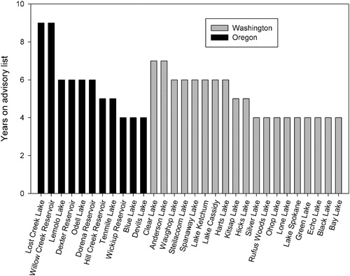
To broadly examine regional relationships between CBs and water quality, lake morphometry, and land use variables in our study, we aimed to include systems chronically affected by hazardous CBs without being limited by dissimilar methods of bloom detection (i.e., cell count or toxin concentration) or dominant cyanobacterial species. The Washington State Toxic Algae and Oregon Public Health Algae Bloom Advisory websites provide lists of systems that have received CB public health advisories issued in accordance with state regulatory guidelines (Washington State Department of Health recreational guidance values and Oregon Health Authority guidance values) based on World Health Organization safety limits for drinking water (WHO 1998) and recreational exposure (WHO 2003). We used these sites to select lakes and reservoirs that repeatedly appeared on advisory lists in both states. We ranked systems according to the total number of years each appeared on a state advisory list, beginning in the year 2005 in Oregon and 2007 in Washington. We used the ranked values to establish a subset as a priority group of systems, hereafter referred to as “affected systems,” defined as lakes or reservoirs receiving CB advisories 4 or more times prior to 2015 (Figure 1). We also selected a set of “unaffected systems,” defined as systems not experiencing CBs, from the 2007 National Lake Assessment (NLA), based on the selection criteria that they (1) have not appeared on either state bloom advisory list, and (2) ranked lowest in the dataset in terms of cyanobacterial cell count densities.

Figure 1. Lakes and reservoirs included in analysis as CB-affected systems. The reported number represents the total number of years each system appeared on a state CB advisory list through the year 2014.

Our dataset included 60 lakes and reservoirs—30 affected systems (11 in Oregon and 19 in Washington) and 30 unaffected systems (15 in Oregon and 15 in Washington; Figs. 1 and 2; Table 1). While additional systems are listed in the CB advisory lists for Washington and Oregon, many of these do not have associated publicly available water quality, lake morphometry, and land use data, and so could not be used in this study. We mapped CB-affected, unaffected, and all other systems listed on Washington and Oregon state CB advisory lists with ArcGIS software to explore spatial patterns of regional CB locations (Fig. 2).

Figure 2. Locations of CB-affected, NLA unaffected, and all other lakes and reservoirs included on Washington (2007–2014) and Oregon (2005–2014) state advisory lists.

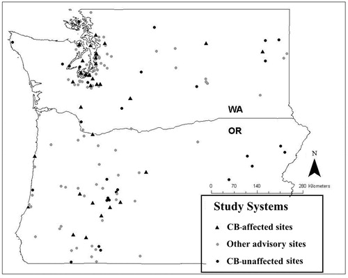
Table 1. CB-affected and unaffected lakes and reservoirs used in regression analysis, listed with state, CB advisory status, and water quality data sources.

Lake name	State	Coordinates	CB advisory	Water quality data source
Rufus Woods Lake	WA	48°3′34″N, 119°19′49″W	affected	NA
Lone Lake	WA	48°1′17″N, 122°27′42″W	affected	Washington State Department of Ecology
Anderson Lake	WA	48°1′11″N, 122°48′6″W	affected	NA
Echo Lake	WA	47°46′17″N, 122°20′35″W	affected	King County
Green Lake	WA	47°40′45″N, 122°20′15″W	affected	King County
Hicks Lake (Garrett, Hicklin)	WA	47°30′12″N, 122°20′42″W	affected	King County
Kitsap Lake	WA	47°34′23″N, 122°42′19″W	affected	Washington State Department of Fish and Wildlife
Bay Lake	WA	47°14′40″N, 122°45′28″W	affected	NA
Clear Lake	WA	46°55′53″N, 122°16′22″W	affected	NA
Harts Lake	WA	46°53′36″N, 122°28′10″W	affected	Washington State Department of Ecology
Ohop Lake	WA	46°53′45″N, 122°16′55″W	affected	Washington State Department of Ecology
Silver Lake	WA	46°17′40″N, 122°47′6″W	affected	Washington State Department of Ecology
Spanaway Lake	WA	47°6′37″N, 122°26′55″W	affected	Washington State Department of Ecology
Steilacoom Lake	WA	47°10′10″N, 122°32′20″W	affected	Washington State Department of Ecology
Waughop Lake	WA	47°10′14″N, 122°33′53″W	affected	Pierce County
Lake Cassidy	WA	48°2′58″N, 122°5′40″W	affected	Snohomish County
Lake Ketchum	WA	48°16′57″N, 122°20′40″W	affected	Snohomish County
Lake Spokane	WA	47°49′53″N, 117°45′42″W	affected	Washington State Department of Ecology
Black Lake	WA	46°59′34″N, 122°58′33″W	affected	Washington State Department of Ecology
Blue Lake	OR	45°33′12″N, 122°26′56″W	affected	Department of Environmental Quality
Devils Lake	OR	44°58′7″N, 124°0′29″W	affected	Atlas of Oregon Lakes
Dexter Reservoir	OR	43°55′14″N, 122°48′14″W	affected	Atlas of Oregon Lakes
Dorena Reservoir	OR	43°47′10″N, 122°57′12″W	affected	Atlas of Oregon Lakes
Hills Creek Reservoir	OR	43°40′10″N, 122°25′27″W	affected	Department of Environmental Quality
Lemolo Lake	OR	43°19′19″N, 122°11′38″W	affected	Atlas of Oregon Lakes
Lost Creek Lake	OR	42°41′23″N, 122°39′19″W	affected	Army Corps of Engineers
Odell Lake	OR	43°34′25″N, 122°0′0″W	affected	Atlas of Oregon Lakes
Tenmile Lake	OR	43°34′11″N, 124°10′2″W	affected	Atlas of Oregon Lakes
Wickiup Reservoir	OR	43°40′59″N, 121°41′30″W	affected	Atlas of Oregon Lakes
Willow Creek Reservoir	OR	44°30′23″N, 120°57′60″W	affected	Atlas of Oregon Lakes
Cle Elum Lake	WA	47°16′1″N, 121°5′38″W	unaffected	National Lake Assessment
Council Lake	WA	46°16′0″N, 121°37′47″W	unaffected	National Lake Assessment
Cranberry Lake	WA	48°23′38″N, 122°39′22″W	unaffected	National Lake Assessment
Cushman Lake	WA	47°29′17″N, 123°15′53″W	unaffected	National Lake Assessment
Horseshoe Lake	WA	45°53′34″N, 122°44′37″W	unaffected	National Lake Assessment
Jump-off Joe Lake	WA	48°8′9″N, 117°41′29″W	unaffected	National Lake Assessment
Lake Koeneman	WA	47°24′34″N, 122°47′4″W	unaffected	National Lake Assessment
Lewis Lake	WA	46°59′11″N, 122°34′9″W	unaffected	National Lake Assessment
Medical Lake	WA	47°34′14″N, 117°41′20″W	unaffected	National Lake Assessment
Mountain Lake	WA	48°39′37″N, 122°49′0″W	unaffected	National Lake Assessment
Ozette Lake	WA	48°5′25″N, 124°37′57″W	unaffected	National Lake Assessment
Rainy Lake	WA	48°30′5″N, 120°44′16″W	unaffected	National Lake Assessment
Red Rock Lake	WA	46°52′17″N, 119°34′15″W	unaffected	National Lake Assessment
Sacheen Lake	WA	48°9′14″N, 117°19′8″W	unaffected	National Lake Assessment
U Lake	WA	47°25′40″N, 123°4′27″W	unaffected	National Lake Assessment
Charlton Lake	OR	43°44′41″N, 121°58′20″W	unaffected	National Lake Assessment
Clear Creek Reservoir	OR	45°3′44″N, 117°9′12″W	unaffected	National Lake Assessment
Clear Lake	OR	45°10′49″N, 121°42′16″W	unaffected	National Lake Assessment
Four Mile Lake	OR	42°28′10″N, 122°15′31″W	unaffected	National Lake Assessment
Hosmer Lake	OR	43°57′49″N, 121°46′50″W	unaffected	National Lake Assessment
Ice Lake	OR	45°13′46″N, 117°16′21″W	unaffected	National Lake Assessment
Lake of the Woods	OR	42°21′54″N, 122°12′51″W	unaffected	National Lake Assessment
Phillips Reservoir	OR	44°40′49″N, 118°2′44″W	unaffected	National Lake Assessment
Smith Reservoir	OR	44°19′0″N, 122°2′47″W	unaffected	National Lake Assessment
Sparks Lake	OR	44°1′36″N, 121°44′44″W	unaffected	National Lake Assessment
Squaw Lakes	OR	42°2′24″N, 123°1′13″W	unaffected	National Lake Assessment
Strawberry Lake	OR	44°18′24″N, 118°41′6″W	unaffected	National Lake Assessment
Torrey Lake	OR	43°47′47″N, 122°1′3″W	unaffected	National Lake Assessment
Van Patten Lake	OR	44°57′15″N, 118°11′10″W	unaffected	National Lake Assessment
Waldo Lake	OR	43°44′10″N, 122°2′17″W	unaffected	National Lake Assessment

Data collection and derivation

Water quality variables that were evaluated for links to CBs included clarity measured by Secchi disk transparency (m), chlorophyll a (µg/L), total phosphorus (TP, µg/L), total nitrogen (TN, mg/L) concentrations, and molar TN:TP ratio. Morphometry variables included drainage area (km²), maximum depth (m), and lake area (ha). We collected data for affected systems using the most recent, publicly available source material, (e.g., water quality reports from local government, the Washington State Department of Ecology water quality monitoring program, and the Atlas of Oregon Lakes). Water quality data for affected systems were collected between 1994 and 2013 in Washington, and between 1981 and 2007 in Oregon. We collected water quality and lake morphometry data for the unaffected systems from the NLA 2007 database. All systems and water quality data sources are listed in Table 1.

We used half-degree resolution output from the Global NEWS-DIP-HD model (Harrison et al. 2010) as a rough indicator of P loading intensity for each of our study systems. The NEWS-DIP-HD model predicts DIP yield (kg/km²/yr) for 5761 watersheds across the globe as a function of land use, nutrient inputs, and hydrology, where P sources include fertilizer, manure, crop harvest, sewage, and detergents (Harrison et al. 2005).

We derived watershed delineations to account for unique contributing areas and land use connected with each study system. We used the National Hydrography Dataset (NHD) to define watersheds and the 2011 National Land Cover Database (NLCD) to determine land use and land cover (LULC) percentages within watersheds of each study system. The NHD includes a nested classification system of watershed boundary delineations that are each assigned a hydrologic unit code (HUC), the scale of which changes from spatially broad at low (e.g., HUC 2) levels to narrow and more defined at higher (e.g., HUC 12) levels. We started our analysis at the HUC 12-digit level, a more local delineation that includes tributary systems. Because boundaries at the HUC 12-digit level did not match the outlets of each study system spatially, we further adjusted the HUC 12 watershed delineations using reference geospatial data, such as NHD rivers, 2011 NLCD and digital elevation models (DEMs; S. 1). LULC percentages within each contributing watershed were calculated in ArcGIS using the NLCD, and 15 of the standard 16 classes were prepared for use in regression analysis. These classes were “developed – open space, developed – low intensity, developed – medium intensity, developed – high intensity, developed land (the sum of all developed classes), barren land (rock/sand/clay), deciduous forest, evergreen forest, mixed forest, shrub/scrub, grassland/herbaceous, pasture/hay, cultivated crops, woody wetlands, and emergent herbaceous wetlands.”

Data analysis

We analyzed the relationships between all water quality, lake morphometry, and LULC variables and CBs using univariate and multiple logistic regressions. Using both types of regression in our analysis enabled us to determine the best model from a combination of all collected data and to test the potential for univariate models to be used as a preliminary means of screening for systems at risk of future CB development. Logistic regression does not depend on assumptions of normality, linearity, or homogeneity of variance for the independent variables, but does require explanatory variables to be independent and a total sample size greater than ∼30. The dependent variable, CB occurrence, was considered a dichotomous outcome and affected systems were assigned a value of “1” while unaffected systems were assigned a value of “0.” Goodness-of-fit for each univariate regression was evaluated using pseudo-r² values, calculated by dividing the residual deviance by the null deviance and subtracting the ensuing quotient from one. Statistics for univariate analyses were completed using Minitab and R Software.

We conducted multiple logistic regression analysis to determine the best combination of environmental and spatial variables with explanatory power for CB predictive models. We tested a total of 24 multiple regression models (Table 2) and evaluated model skill using modified R² values. We evaluated the tradeoff between model simplicity and model skill using the Akaike information criterion (AIC; Tjur 2009). After we determined significant predictors from each category of variables (i.e., water quality, morphometry, and LULC), we continued to test for the best multiple category model starting with the following equation: $$CB=a\mathrm{*}\left(\mathit{\text{Developed}}-\mathit{\text{Open}}\mathrm{}\mathit{\text{Space}}\right)+b\mathrm{*}\left(\mathit{\text{Evergreen}}\mathrm{}\mathit{\text{forest}}\right)+c\mathrm{*}\left(\mathit{\text{Scrub}}\mathrm{}\mathit{\text{shrub}}\right)+d\mathrm{*}\left(\mathit{\text{Grassland}}\mathrm{}\mathit{\text{herbaceous}}\right)+e\mathrm{*}\left(\mathit{\text{Pasture}}\mathrm{}hay\right)+f\mathrm{*}\left(TN\right)+g\mathrm{*}\left(TP\right)+h\mathrm{*}\left(Chl\mathrm{-}a\right)+j\mathrm{*}\left(\mathit{\text{Drai}}nage\mathrm{}\mathit{\text{area}}\right),$$ where a through j are parameter estimates for each variable included in the model (Table 2). The explanatory variables a through e were percentages of watershed land cover in the LULC category, f through h were measures in the water quality category, and j was in the lake morphometry category. We then used a backwards stepwise AIC optimization technique to remove variable combinations sequentially until the final best model included only those with the smallest AIC and P values. Due to missing data for specific systems, the sample size for the initial best model started with 39 observations and increased to 54 observations. We conducted multiple logistic regression analysis using R software.

Table 2. Significance results (P values) for all variables tested in multiple logistic regression analysis and performance results for all models tested (AIC and R² values) and used in development of a final multi-category model. An “X” indicates a variable that was included in an initial model but was removed during AIC optimization.

	Land Use	Developed	Land Cover	Water Quality	Lake Morphometry	Chl-a	Initial Best Fit	Final Best Fit (1)	Final Best Fit (2)
Drainage area					0.071		0.059	0.005	0.008
Depth, maximum					X
Lake area					X
Clarity (Secchi disk)				X
Chl-a				X		0.005	0.928	X	X
TP				0.034			0.248	0.052	0.003
Modeled DIP yield				X
TN				0.018			0.256	X	X
N:P ratio				0.023			X
Developed – open space	0.032						0.799	0.008	X
Developed – low intensity	X
Developed – medium intensity	X
Developed – high intensity	X
Developed – all		0.021
Barren land			X
Deciduous forest			X
Evergreen forest			0.003				0.149	X	0.019
Mixed forest			X
Shrub/scrub			0.153				0.882	X	X
Grassland/herbaceous			0.070				0.516	X	X
Pasture/hay			0.084				0.126	X	X
Cultivated crops			X
Woody wetlands			X
Emergent herbaceous wetlands			X
AIC	77.506	76.523	79.290	30.918	72.743	45.073		47.665	54.023
R^2 (modified)	0.230	0.153	0.211	0.583	0.131	0.455		0.529	0.440

Pearson’s correlation analysis was conducted on all 27 variables to analyze collinearity and determine which variable combinations were not appropriate for multivariate models. Variables with a strong correlation (≥0.5) are shown in Table 3. A total of 33 systems with complete datasets were used in the correlation analysis due to missing data.

Table 3. Results of pairwise Pearson’s correlation analysis of water quality, lake morphometry, and land use data used in logistic regression analysis. Correlation values are shown only for those variables with a strong correlation (≥0.5).

	Max lake depth	Lake area	Total watershed area	Total nitrogen	Cultivated crops	Modeled DIP yield	Developed – low intensity	Developed – med. intensity	Developed – high intensity	Mixed forest	Evergreen forest	Grassland herbaceous
Contributing area	0.56	0.63	0.78
Pasture hay				0.57	0.78			0.5	0.65		−0.51
Deciduous forest						0.66				0.85
Shrub scrub												0.51
Developed – open space							0.84	0.72	0.5
Developed – medium intensity							0.97	1	0.91
Developed – high intensity							0.79	0.91	1
Barren land											−0.51
Mixed forest						0.77				1
Cultivated crops				0.85	1
Total watershed area		0.53	1
N:P ratio					0.52

We developed an inventory of at-risk systems using the remaining 39 Washington and Oregon lakes in the NLA dataset not included in our regression analysis to demonstrate a possible use of simplistic univariate models in preliminary screenings of lake and reservoir risk assessment. A predicted probability of CB occurrence was calculated for each of the screened NLA systems using the univariate [Chl-a] logistic regression model and max Chl-a value from each system. We identified at-risk systems amongst NLA lakes as those with a probability of bloom occurrence ≥0.5. We selected only the [Chl-a] model for use in a preliminary screening example because it had the greatest pseudo-r² of all univariate models.

Results

Regional distribution of blooms

Examination of mapped CB advisory locations revealed that affected systems in Washington are concentrated largely in the urban area around Puget Sound, with fewer affected systems reported in the central and eastern part of the state (Fig. 2). In Oregon, affected systems are clustered almost entirely on the western side of the state.

Univariate logistic regression

Water quality variables that significantly related to CBs according to univariate logistic regression analysis (Table 4) included [Chl-a] (P = 0.005, pseudo-r² = 0.39), [TP] (P = 0.005, pseudo-r² = 0.16), clarity (P = 0.022, pseudo-r² = 0.13), and modeled DIP yield (P = 0.011, pseudo-r² = 0.20). LULC variables significantly related to CBs included “developed – open space” (P = 0.003, pseudo-r² = 0.17), “developed – low intensity” (P = 0.023, pseudo-r² = 0.11), “evergreen forest” (P = 0.011, pseudo-r² = 0.09), and “mixed forest” (P = 0.014, pseudo-r² = 0.19). The variable “barren land” was also significantly (although weakly) related to CB outcome (P = 0.048, pseudo-r² = 0.15). “Evergreen forest,” “barren land,” and water clarity were inversely related, while all other variables were positively related, to CBs. None of the morphometry variables were significantly related to CB occurrence in univariate models; the water quality variables TN and N:P ratio were also not significantly related to CB occurrence.

Table 4. Univariate logistic regression results for all water quality, lake morphometry, and land use variables.

Metric tested	n	Estimate	Std. error	P	pseudo-r^2
Max depth	58	7.61 × 10^−3	1.25 × 10^−2	0.544
Lake area	59	1.50 × 10^−4	3.23 × 10^−4	0.642
Drainage area	56	3.0 × 10^−3	1.67 × 10^−3	0.071
Developed – open space	60	29.6	10.1	0.003**	0.17
Developed – low intensity	60	9.88	4.33	0.023*	0.011
Developed – medium intensity	60	8.92	5.37	0.097
Developed – high intensity	60	20.9	12.4	0.091
Percent cultivated crops	60	−4.35	6.26	0.487
Percent woody wetlands	60	8.04	8.48	0.343
Evergreen forest	60	−2.44	0.963	0.011*	0.085
Percent pasture	60	−1.44	5.01	0.774
Percent grassland	60	−4.32	5.93	0.466
Barren land	60	−39.2	19.8	0.048*	0.15
Mixed forest	60	27.5	11.2	0.014*	0.19
Deciduous forest	60	130.6	71.3	0.067
Herbaceous wetland	60	4.62	13.6	0.734
Modeled DIP yield	60	0.026	0.0103	0.011*	0.20
Clarity (Secchi disk)	50	−0.252	0.11	0.022*	0.13
Chlorophyll a	50	0.162	0.058	0.005**	0.39
Total Phosphorus (TP)	55	0.051	0.018	0.005**	0.16
Total Nitrogen (TN)	43	0.897	0.683	0.189
N:P	43	−0.104	0.057	0.071

Significance codes: *** = 0.001, ** = 0.01, * = 0.05.

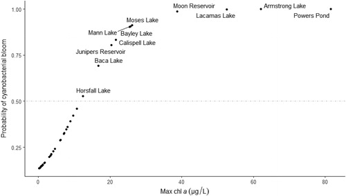
We identified a list of 11 systems that may be at risk for developing CBs in the future by screening Chl-a concentrations from additional lakes in the NLA database (Fig. 3). Model results predict an elevated risk (probability ≥0.5) of a CB in systems with a max Chl-a of ∼12 µg/L and extreme risk (probability approaches 1) when Chl-a levels ≥30 µg/L. Based on results of our univariate [Chl-a] model, these 11 systems are more likely than not (≥ 0.5) to experience future CBs and should be included in monitoring programs where human exposure is likely, or be considered a priority for expanded future ecosystem monitoring efforts.

Figure 3. Systems predicted to be at high risk of developing future CBs based on a preliminary screening of NLA systems using the Chl-a–based univariate model for a probability of >0.5. Line used to label Mann Lake due to overlapping data points for systems with similar values.

Multiple logistic regression

Multiple logistic regression analysis produced 2 best-fit models (Table 5) for CB occurrence as a result of stepwise AIC optimization. “Final Best Fit 1” was the stronger model, with a higher modified r² and lower AIC value (AIC = 47.665, modified r² = 0.529), and included the predictor variables “developed – open space” (P = 0.008), TP (P = 0.052), and “drainage area” (P = 0.005). The second model (AIC = 54.023, modified r² = 0.440) included “evergreen forest” (P = 0.019), TP (P = 0.003), and “drainage area” (P = 0.008). Considering both models provides additional insight regarding important variables associated with CBs. Parameter estimates for these 2 models suggest that the LULCs “developed – open space” (40.88) and “evergreen forest” (−3.25) best predict CB locations of all the explanatory variables tested (Table 5). Confidence intervals for multivariate model intercepts and variables are reported (Table 6). All significant predictor variables included in final multivariate models were positively related to CB occurrence except for “evergreen forest” and “barren land,” which were inversely related to CB occurrence.

Table 5. Parameter results for the 2 final multiple logistic regression models predicting CB occurrence developed from water quality, lake morphometry, and land use factors.

Variable	Estimate	Std. error	z value	Pr(>|z|)
Model 1: AIC = 47.665, modified R^2 = 0.529
Intercept	−3.38	0.924	−3.667	2.46 × 10^−4***
Developed – open space (%)	40.8	15.3	2.67	7.58 × 10^−3**
TP	0.0419	0.0216	1.94	0.052
Drainage area (km^2)	6.02 × 10^−3	2.14 × 10^−3	2.81	0.005**
Model 2: AIC 54.023, modified R^2 0.440
Intercept	−1.02	0.757	−1.35	0.177
Evergreen forest (%)	−3.25	1.38	−2.34	0.019*
TP	5.99 × 10^−2	0.020	2.95	0.003**
Drainage area (km^2)	5.9 × 10^−3	2.23 × 10^−3	2.64	0.008**

Significance codes: *** = 0.001, ** = 0.01, * = 0.05.

Table 6. Confidence interval estimates for variables included in multiple logistic regression models.

	Final Best Fit (1) confidence intervals		Final Best Fit (2) confidence intervals
Variables with estimates	2.5%	97.5%	2.5%	97.5%
Intercept	−5.57	−1.83	−2.60	0.425
Developed – open space (%)	15.3	76.8
TP	3.39 × 10^−3	8.85 × 10^−2	0.0238	0.105
Drainage area (km^2)	8.85 × 10^−2	1.01 × 10^−2	2.15 × 10^−3	1.11 × 10^−2
Evergreen forest (%)			−6.28	−0.724

Discussion

We created a map of CB advisory systems in Oregon and Washington as part of our exploratory analysis. The clustered pattern of CB advisory locations around Puget Sound in Washington and on the western side of Oregon is consistent with the distribution of developed LULCs our study found to be associated with CBs. These patterns may reflect the true distribution of CBs, but it is also likely that underreporting is a contributing factor. For example, bloom monitoring programs may be more rigorous in some counties, such as the SoundToxins and Freshwater Algae Control programs conducted in Puget Sound and King County, Washington (Trainer and Hardy 2015), while in other locations blooms are not being observed and reported.

Our main objectives were to find those water quality, morphometry, and LULC variables most strongly associated with systems experiencing frequent CBs and to create a regional model to explain CB occurrence and for use as a screening tool for freshwater systems at high risk of developing such blooms. To find the simplest and most useful model, we analyzed data using univariate and multiple logistic regressions. Multiple water quality (i.e., [Chl-a], TP, clarity, and DIP yield) and LULC (i.e., “evergreen forest,” “developed – open space,” “developed – low intensity,” “mixed-forest,” and “barren land”) variables were significantly related to CB occurrence according to our analyses and may therefore prove useful in CB predictive models. Of these, TP, “evergreen forest,” and “developed – open space” were also significant variables in multiple regression models. LULC “drainage area” was the only variable significantly related to CB occurrence in multivariate (P = 0.008) but not univariate (P = 0.07) models.

Our simple univariate regression results provide an example of how simple models can be employed as part of an early CB risk assessment. Chl-a concentration, despite not being wholly specific to cyanobacteria among phytoplankton populations, explained the most variance of all univariate regression models (pseudo-r² = 0.39). Other studies have noted a shift in phytoplankton community composition toward an increasing dominance by cyanobacteria in highly eutrophic systems (Watson et al. 1997, Havens 2008). This relationship may help explain our results regarding the explanatory power of [Chl-a] in cyanobacterial bloom detection, further supporting its use as a “first step” in CB lake risk assessment. As an example, we used the [Chl-a] model to screen for systems with a high probability (>0.5) of developing CBs in the future (Fig. 3). This method of screening, while fast and simple, may benefit resource managers by helping them focus efforts on high risk systems for more cost-effective monitoring.

Results from both simple and multiple regression approaches suggest that TP has particular value for CB modeling and prediction. Phosphorus has long been known as a key nutrient for freshwater phytoplankton growth (Wetzel 2001, Reynolds 2006, Schindler et al. 2008) and CBs (Conley et al. 2009, Paerl and Otten 2013). While N and P are both recognized as key factors for CB formation (Sterner 2008, Conley et al. 2009, Paerl et al. 2011, Paerl et al. 2016), our results indicate that TP is more useful as a bloom predictor than TN or N:P in these study systems. Other researchers have found similar results. TP has been used to predict cyanobacterial biomass (Smith 1985, Smith et al. 1987) and has more recently been found to outperform TN (Jensen et al. 1994, Håkanson et al. 2007) or even N:P (Jensen et al. 1994, Downing et al. 2001, Håkanson et al. 2007) as a CB predictor. The N:P ratio has, however, been significantly related to cyanobacteria in other studies, notably revealing a relationship between N:P ratios and microcystin concentration in lakes throughout Canada and Washington State (Orihel et al. 2012, Jacoby et al. 2015). Also consistent with our findings, other studies in the PNW found that TP correlated with CBs in 2 PNW lakes with multi-year records (Jacoby et al. 2000, Johnston and Jacoby 2003).

As significant predictors of CBs, both DIP yield and [Chl-a] data can be used to help assess lake risk of CB formation. Because DIP is the orthophosphate portion of TP and is thus entirely available for phytoplankton growth (Reynolds and Davies 2001, O’Neil et al. 2012), it is likely a reasonable indicator of a system’s potential to develop and sustain CBs. While not as direct as in-lake measurements, modeled DIP yield provides an estimate of how much bioavailable phosphorus moves through a watershed. High model-predicted watershed DIP yield is an indicator that P loading is likely to be high, driving eutrophication of lakes and reservoirs. Using modeled DIP yield as a proxy for in-system measurements has some drawbacks, including the potential for overestimating or underestimating concentrations and simplifying nutrient transport and in-system dynamics. While future CB models may improve upon our approach by using measurement-based estimates of DIP concentration and/or yield, our results indicate that model-derived estimates of DIP yield may help identify systems at risk of experiencing blooms.

Drainage area and land use classes “developed – open space,” “developed – low intensity,” “evergreen forest,” “barren land,” and “mixed forest” were significantly related to CBs according to one or both model types. A larger drainage area may result in increased nutrient availability to fuel CBs. All other climate, watershed, and lake size factors being equal, the amount of water and nutrients flushed into lakes increases with drainage area. This larger inflow has the potential to fuel phytoplankton growth thereby increasing risk of frequent CBs, especially in agriculturally dominated watersheds (Anderson et al. 2002, Davis et al. 2009, Michalak et al. 2013). “Developed – open space,” significant in both model types, includes green spaces such as lawns, parks, and golf courses, which may increase eutrophication and CBs if fertilizer is being over- or mis-applied (e.g., before heavy rain). “Evergreen forest” and “barren land” were negatively related to CB occurrence. Forested land is known to retain nutrients (Likens et al. 1970, Lowrance et al. 1984, Matteo et al. 2006, Jose 2009), which may reduce nutrient inputs to freshwater systems in highly forested watersheds—a potential that should be explored in future CB mitigation studies.

Research needs and conclusions

While conducting this study, we identified data needs limiting broad-scale analyses. Lack of available water quality data limited the number and type of systems we could include in this analysis. Restricting sample size allowed us to develop a more detailed dataset of potential drivers for each lake but may have reduced model power and accuracy. Access to additional water quality data is critical for improvement of future CB modeling.

CB prediction models would also benefit from increased resolution of input variables from nutrient transport models and watershed LULC characteristics. One caveat of LULC analysis was that focus was solely on composition (e.g., percentage), not on arrangement or location of specific land uses (e.g., proximity of forest to water bodies). Further spatial analysis could include tests for autocorrelation between pairs of lake systems to understand if one lake may influence another or if larger-scale landscape or climate characteristics influence co-located systems similarly.

Natural resource managers and municipalities need predictive models that facilitate a more targeted monitoring of systems at risk of developing CBs. Frequently, financial and/or time constraints may require sampling of only one or two metrics when assessing water quality. That reality, together with the desire to create a simple but effective model, provides sound reason to test univariate in addition to multivariate models. While CBs are, in actuality, the result of many rapidly fluctuating factors (O’Neil et al. 2012, Paerl and Otten 2013, Paerl et al. 2016, Pick 2016), our results support the use of DIP yield, [Chl-a], and TP together with prominent LULCs, most notably “developed – open space” and “evergreen forest,” as a first step in CB prediction. The significant relationships observed here between water quality variables such as Chl-a, water clarity, and TP and CBs are consistent with prior studies; however, the strong relationships between CBs and LULC factors and modeled DIP yield are not as well established. Our study provides support for use of these variables as part of ongoing CB predictive model development and suggests particular relevance due to a lack of available, current water quality data. Further, due to the significance of TP in both univariate and multivariate models, our results support reduction of P inputs as a key CB mitigation strategy for freshwater systems in the PNW, consistent with other studies (Schindler 2006, Carpenter 2008, O’Neil et al. 2012).

Acknowledgments

We thank the Washington and Oregon state departments for compiling and making available data on systems affected by CBs, which made this research possible.

Additional information

Funding

This work was supported by grants from the NSF Ecosystem Science (DEB1355211), NSF INFEWS (EAR1639458), the USDA/NIFA Water Sustainability and Climate program (20126700319805), and the USGS 104 b program to JAH, and a NSF Graduate Research Fellowship Program grant (1347973) to VJR.

References

- Allan JD. 2004. Landscapes and riverscapes: the influence of land use on stream ecosystems. Annu Rev Ecol Evol Syst. 35(1):257–284.
- Anderson DM, Glibert PM, Burkholder JM. 2002. Harmful algal blooms and eutrophication: nutrient sources, composition, and consequences. Estuaries. 25(4):704–726.
- Beaulieu M, Pick F, Palmer M, Watson S, Winter J, Zurawell R, Gregory-Eaves I. 2014. Comparing predictive cyanobacterial models from temperate regions. Can J Fish Aquat Sci. 71(12):1830–1839.
- Carpenter SR. 2008. Phosphorus control is critical to mitigating eutrophication. Proc Natl Acad Sci USA. 105(32):11039–11040.
- Codd GA, Lindsay J, Young FM, Morrison LF, Metcalf JS. 2005. Harmful cyanobacteria. In: Huisman J, Matthijs HCP, Visser PM, editors. Harmful cyanobacteria. Dordrecht (The Netherlands): Springer. p. 1–23.
- Conley DJ, Paerl HW, Howarth RW, Boesch DF, Seitzinger SP, Havens KE, Lancelot C, Likens GE. 2009. Ecology - controlling eutrophication: nitrogen and phosphorus. Science. 323(5917):1014–1015.
- Cooper CM. 1993. Biological effects of agriculturally derived surface water pollutants on aquatic systems - a review. J Environ Qual. 22(3):402–408.
- Davis TW, Berry DL, Boyer GL, Gobler CJ. 2009. The effects of temperature and nutrients on the growth and dynamics of toxic and non-toxic strains of Microcystis during cyanobacteria blooms. Harmful Algae. 8(5):715–725.
- Downing JA, Watson SB, McCauley E. 2001. Predicting cyanobacteria dominance in lakes. Can J Fish Aquat Sci. 58(10):1905–1908.
- Elliott JA. 2012. Is the future blue-green? A review of the current model predictions of how climate change could affect pelagic freshwater cyanobacteria. Water Res. 46(5):1364–1371.
- Glibert PM, Anderson DM, Gentien P, Graneli E, Sellner KG. 2005. The global, complex phenomena of harmful algal blooms. Oceanography. 18(2):136–147.
- Glibert PM, Seitzinger S, Heil CA, Burkholder JM, Parrow MW, Codispoti LA, Kelly V. 2005. The role of eutrophication in the global proliferation of harmful algal blooms: new perspectives and new approaches. Oceanography. 18(2):198–209.
- Håkanson L, Bryhn AC, Hytteborn JK. 2007. On the issue of limiting nutrient and predictions of cyanobacteria in aquatic systems. Sci Total Environ. 379(1):89–108.
- Harrison JA, Bouwman AF, Mayorga E, Seitzinger S. 2010. Magnitudes and sources of dissolved inorganic phosphorus inputs to surface fresh waters and the coastal zone: a new global model. Global Biogeochem Cycles. (1). doi: 10.1029/2009GB003590.
- Harrison JA, Seitzinger SP, Bouwman AF, Caraco NF, Beusen AHW, Vörösmarty CJ. 2005. Dissolved inorganic phosphorus export to the coastal zone: results from a spatially explicit, global model. Global Biogeochem Cycles. 19(4). doi: 10.1029/2004GB002357.
- Havens KE. 2008. Cyanobacteria blooms: effects on aquatic ecosystems. In: Hudnell HK, editor. Cyanobacterial harmful algal blooms: state of the science and research needs. Advances in experimental medicine and biology, vol. 619. New York (NY): Springer. p. 733–747.
- Heisler J, Glibert P, Burkholder J, Anderson D, Cochlan W, Dennison W, Gobler C, Dortch Q, Heil C, Humphries E, et al. 2008. Eutrophication and harmful algal blooms: a scientific consensus. Harmful Algae. 8(1):3–13.
- Hoagland P, Anderson DM, Kaoru Y, White AW. 2002. The economic effects of harmful algal blooms in the United States: estimates, assessment issues, and information needs. Estuaries. 25(4):819–837.
- Huisman J, Matthijs HCP, Visser PM, editors. 2005. Harmful cyanobacteria. Aquatic ecology series. Dordrecht (The Netherlands): Springer.
- Jacoby JM, Burghdoff M, Williams G, Read L, Hardy FJ. 2015. Dominant factors associated with microcystins in nine midlatitude, maritime lakes. IW. 5(2):187–202.
- Jacoby JM, Collier DC, Welch EB, Hardy FJ, Crayton M. 2000. Environmental factors associated with a toxic bloom of Microcystis aeruginosa. Can J Fish Aquat Sci. 57(1):231–240.
- Jacoby JM, Kann J. 2007. The occurrence and response to toxic cyanobacteria in the Pacific Northwest, North America. Lake Reserv Manage. 23(2):123–143.
- Jensen JP, Jeppesen E, Olrik K, Kristensen P. 1994. Impact of nutrients and physical factors on the shift from cyanobacterial to chlorophyte dominance in shallow Danish lakes. Can J Fish Aquat Sci. 51(8):1692–1699.
- Johnston BR, Jacoby JM. 2003. Cyanobacterial toxicity and migration in a mesotrophic lake in western Washington, USA. Hydrobiologia. 495:79–91.
- Jose S. 2009. Agroforestry for ecosystem services and environmental benefits: an overview. Agroforest Syst. 76(1):1–10.
- Leigh C, Burford MA, Roberts DT, Udy JW. 2010. Predicting the vulnerability of reservoirs to poor water quality and cyanobacterial blooms. Water Res. 44(15):4487–4496.
- Lewis WM, Wurtsbaugh WA, Paerl HW. 2011. Rationale for control of anthropogenic nitrogen and phosphorus to reduce eutrophication of inland waters. Environ Sci Technol. 45(24):10300–10305.
- Likens GE, Bormann FH, Johnson NM, Fisher DW, Pierce RS. 1970. Effects of forest cutting and herbicide treatment on nutrient budgets in the Hubbard Brook watershed ecosystem. Ecol Monogr. 40(1):23–47.
- Lowrance R, Todd R, Fail J, Hendrickson O, Leonard R, Asmussen L. 1984. Riparian forests as nutrient filters in agricultural watersheds. BioScience. 34(6):374–377.
- Matteo M, Randhir T, Bloniarz D. 2006. Watershed-scale impacts of forest buffers on water quality and runoff in urbanizing environment. J Water Resour Plann Manage. 132(3):144–152.
- Michalak AM, Anderson EJ, Beletsky D, Boland S, Bosch NS, Bridgeman TB, Chaffin JD, Cho K, Confesor R, Daloglu I, et al. 2013. Record-setting algal bloom in Lake Erie caused by agricultural and meteorological trends consistent with expected future conditions. Proc Natl Acad Sci USA. 110(16):6448–6452.
- O’Neil JM, Davis TW, Burford MA, Gobler CJ. 2012. The rise of harmful cyanobacteria blooms: the potential roles of eutrophication and climate change. Harmful Algae. 14:313–334.
- Orihel DM, Bird DF, Brylinsky M, Chen H, Donald DB, Huang DY, Giani A, Kinniburgh D, Kling H, Kotak BG, et al. 2012. High microcystin concentrations occur only at low nitrogen-to-phosphorus ratios in nutrient-rich Canadian lakes. Can J Fish Aquat Sci. 69(9):1457–1462.
- Paerl HW, Gardner WS, Havens KE, Joyner AR, McCarthy MJ, Newell SE, Qin B, Scott JT. 2016. Mitigating cyanobacterial harmful algal blooms in aquatic ecosystems impacted by climate change and anthropogenic nutrients. Harmful Algae. 54:213–222.
- Paerl HW, Huisman J. 2009. Climate change: a catalyst for global expansion of harmful cyanobacterial blooms. Env Microbiol Rep. 1(1):27–37.
- Paerl HW, Otten TG. 2013. Harmful cyanobacterial blooms: causes, consequences, and controls. Microb Ecol. 65(4):995–1010.
- Paerl HW, Xu H, McCarthy MJ, Zhu G, Qin B, Li Y, Gardner WS. 2011. Controlling harmful cyanobacterial blooms in a hyper-eutrophic lake (Lake Taihu, China): the need for a dual nutrient (N & P) management strategy. Water Res. 45(5):1973–1983.
- Pick FR. 2016. Blooming algae: a Canadian perspective on the rise of toxic cyanobacteria. Can J Fish Aquat Sci. 73(7):1149–1158.
- Reynolds CS. 2006. Ecology of phytoplankton. Cambridge (UK); New York (NY): Cambridge University Press.
- Reynolds CS, Davies PS. 2001. Sources and bioavailability of phosphorus fractions in freshwaters: a British perspective. Biol Rev Camb Philos Soc. 76(1):27–64.
- Robb M, Greenop B, Goss Z, Douglas G, Adeney J. 2003. Application of PhoslockTM, an innovative phosphorus binding clay, to two Western Australian waterways: preliminary findings. In: Kronvang B, editor. The Interactions between Sediments and Water. Dordrecht (The Netherlands): Springer. p. 237–243.
- Schindler DW. 2006. Recent advances in the understanding and management of eutrophication. Limnol Oceanogr. 51(1, part 2):356–363.
- Schindler DW, Hecky RE, Findlay DL, Stainton MP, Parker BR, Paterson MJ, Beaty KG, Lyng M, Kasian SEM. 2008. Eutrophication of lakes cannot be controlled by reducing nitrogen input: results of a 37-year whole-ecosystem experiment. Proc Natl Acad Sci USA. 105(32):11254–11258.
- Smith VH. 1983. Low nitrogen to phosphorus ratios favor dominance by blue-green algae in lake phytoplankton. Science. 221(4611):669–671.
- Smith VH. 1985. Predictive models for the biomass of blue-green algae in lakes. J Am Water Resources Assoc. 21(3):433–439.
- Smith VH, Willén E, Karlsson B. 1987. Predicting the summer peak biomass of four species of blue-green algae (cyanophyta/cyanobacteria) in Swedish lakes. J Am Water Resources Assoc. 23(3):397–402.
- Sterner RW. 2008. On the phosphorus limitation paradigm for lakes. Internat Rev Hydrobiol. 93(4–5):433–445.
- Stewart I, Seawright AA, Shaw GR. 2008. Cyanobacterial poisoning in livestock, wild mammals and birds–an overview. In: Cyanobacterial harmful algal blooms: state of the science and research needs. New York (NY): Springer. p. 613–637.
- Tjur T. 2009. Coefficients of determination in logistic regression models—a new proposal: the coefficient of discrimination. Am Stat. 63(4):366–372.
- Trainer VL, Hardy FJ. 2015. Integrative monitoring of marine and freshwater harmful algae in Washington State for public health protection. Toxins (Basel). 7(4):1206–1234.
- Trimbee AM, Prepas EE. 1987. Evaluation of total phosphorus as a predictor of the relative biomass of blue-green algae with emphasis on Alberta Lakes. Can J Fish Aquat Sci. 44(7):1337–1342.
- Vitousek PM, Aber JD, Howarth RW, Likens GE, Matson PA, Schindler DW, Schlesinger WH, Tilman DG. 1997. Human alteration of the global nitrogen cycle: sources and consequences. Ecol Appl. 7:737–750.
- Watson SB, McCauley E, Downing JA. 1997. Patterns in phytoplankton taxonomic composition across temperate lakes of differing nutrient status. Limnol Oceanogr. 42(3):487–495.
- Wetzel RG. 2001. Limnology: lake and river ecosystems. 3rd ed. San Diego (CA): Academic Press.
- [WHO] World Health Organization. 1998. Guidelines for drinking water quality. 2nd ed., Addendum to Volume 2, Health Criteria and Other Supporting Information. Geneva (Switzerland).
- [WHO] World Health Organization. 2003. Guidelines for safe recreational water environments. Coastal and Fresh Waters. Vol. 1. Geneva (Switzerland).