Variability in the vertical distribution of chlorophyll in a spill-managed temperate reservoir

Abstract

Perkins KR, Rollwagen-Bollens G, Bollens SM, Harrison JA. 2019. Variability in the vertical distribution of chlorophyll in a spill-managed temperate reservoir. Lake Reserve Manage. 35:119–126.

Phytoplankton form the base of pelagic food webs, and as aquatic systems come under increasing pressure from environmental stressors, managers are becoming more concerned about how these pressures may result in changes to phytoplankton distribution and abundance. The vertical distribution of phytoplankton, including the phenomenon of subsurface chlorophyll a (Chl-a) maxima (SCM), is known to vary widely, with a combination of biotic and abiotic processes hypothesized to be driving this variation. We examined how the vertical distribution of Chl-a generally, and SCM specifically, varied over 4 years (2013–2016) in a managed temperate reservoir (Lacamas Lake, Washington, USA) that experiences rapid (2–3 weeks) release of water from within the epilimnion each autumn. Seasonally, a strong thermocline developed each spring at depths of 5–10 m, and persisted throughout summer and early autumn. Although temperature varied somewhat between years, elevated concentrations of Chl-a occurred in spring and summer of each year. In addition, pronounced SCM of 30–60 µg/L at depths of 2–8 m were observed each year, and were nearly always above the thermocline. There was no “seasonal deepening” of SCM in Lacamas Lake, as has been observed in several other lakes and oceans, and annual drawdown events in early fall had little to no effect on SCM in Lacamas Lake. We recommend that more process-oriented studies be undertaken to fully understand which biotic and abiotic processes are driving the formation and maintenance of SCM in lakes and reservoirs, and how SCM are modulated by different reservoir drawdown practices.

Keywords:

• Drawdown effects
• phytoplankton
• reservoir
• seasonal deepening
• size-fractionation
• subsurface chlorophyll maxima
• vertical distribution

The composition and vertical distribution of phytoplankton in marine and freshwater systems are affected by abiotic and biotic factors, including water column stratification and the availability of light and nutrients, as well as processes such as sinking and grazing in the water column (Reynolds 2006). The result of these processes is often vertical heterogeneity (e.g., layers or patches) of chlorophyll a (Chl-a) concentration (Abbott et al. 1984; Bochdansky and Bollens 2009). Frequently, Chl-a maxima occur in surface waters where light availability is greatest; however, subsurface Chl-a maxima (SCM) have been recorded extensively in oceans (Bienfang et al. 1984; Martin et al. 2010; Mignot et al. 2014), estuaries (Alldredge et al. 2002; Menden-Deuer 2008; Bochdansky and Bollens 2009), natural lakes (Abbott et al. 1984; Barbiero and Tuchman 2004; Leach et al. 2018), and reservoirs (Chapin et al. 2004; deNoyelles et al. 2016; Mineeva and Mukhutdinov 2018). There is a growing recognition that a combination of biotic and abiotic processes is likely interact to create and maintain SCM (Cullen 2015).

The phenomenon of SCM has been much more extensively studied in marine versus freshwater systems. For instance, a search on Web of Science for papers published between 1980 and 2017 conducted with the keywords (“marine” OR “ocean”) AND (“subsurface chlorophyll maxim*” OR “deep chlorophyll maxim*”) produced 1,169 results. A search conducted with the keywords (“freshwater” OR “reservoir”) AND (“subsurface chlorophyll maxim*” OR “deep chlorophyll maxim*”) produced 346 results, or less than 30% of the number of studies in marine systems. This begs the question of whether SCM are actually less common in freshwater systems, or whether there has simply been less effort to investigate them in freshwater systems.

Even less attention has been directed toward understanding SCM in the context of reservoir management. This represents a critical gap in our understanding of phytoplankton populations in reservoirs, since the operation of dams to manage reservoirs may have substantial impact on total water volume, reservoir depth and water flows. In particular, the release of water over and/or through dams may affect the vertical distribution of phytoplankton (as indicated by Chl-a) in reservoirs.

Over the past century, alteration of river flow via the construction of more than 1 million dams and reservoirs worldwide has profoundly altered physical and biological characteristics of rivers and their watersheds (Harrison et al. 2009; Lehner et al. 2011; Harrison et al. 2012; Deemer et al. 2016). These effects are likely to increase, as new dam construction in developing countries could double the number of large dams globally (Zarfl et al. 2015). Despite the clear and increasing importance of managed waters, the effects of reservoir drawdown as a result of dam management operations on phytoplankton distribution in reservoirs are not well understood. Interactions between reservoir management and phytoplankton dynamics are particularly important to understand as the frequency of algal blooms in reservoirs is increasing, often leading to degradation of water quality and higher vulnerability of drinking water for human populations (Paerl 2008; Paerl and Otten 2013).

Thus, we were led to investigate the following two research questions:

1. How does the vertical distribution of Chl-a generally, and the subsurface Chl-a maximum (SCM) specifically, vary over time in a temperate reservoir?

2. Do dam management operations that result in an annual rapid water level drawdown from within the epilimnion affect the vertical distribution of Chl-a?

Study site

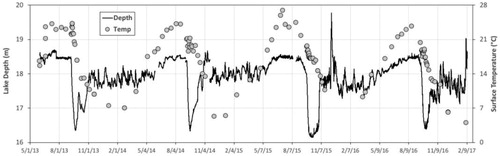
Lacamas Lake is a small (1.3 km²) reservoir located in the southwest corner of Washington State, USA (45.37 N, 122.25W). The lake, which was dammed in 1938, has an average depth of 7.8 m and a maximum depth of 19.8 m (Deemer et al. 2015). The watershed of the lake includes forested uplands, agricultural lands, and suburban development—the latter two having contributed to eutrophication of the lake (Deemer et al. 2011). Lacamas Lake is strongly stratified from June to October and experiences hypolimnetic hypoxia annually during summer months (Deemer et al. 2015). Water in Lacamas Lake is drawn down annually in the fall through an outlet located at ∼2 m depth for mechanical maintenance of the dam structure, which decreases lake depth by approximately 2 m and lake volume by 20–40% within a 2- to 4-week period. This relatively abrupt drawdown contrasts with some other reservoirs that have a more protracted drawdown over several months. Following drawdown, the lake then refills naturally as precipitation increases through the fall and winter (Deemer et al. 2011; Figure 1).

Figure 1. Surface temperature and water depth measured at the sampling site in Lacamas Lake, Washington from May 2013 to February 2017.

Materials and methods

Sample collection and processing

Vertical profiles of temperature and fluorescence (a proxy measure of Chl-a) were collected with a Hach DS5X Sonde near the deepest point of the lake (∼18 m) biweekly during spring, summer and autumn, daily during drawdown periods, and less frequently (generally monthly to bimonthly) during winter, from May 2013 to February 2017. Data were collected at the following depths: 0.1, 1, 2, 4, 5.5, 7, 9, 13, 15 m, and immediately above the lake bottom. On an approximately bi-monthly basis over the 4-year sampling period, fluorescence values measured with the Sonde were compared to a solid state Chl-a standard. On 2 occasions (September and October 2015) the solid state standard was compared with acetone-digested water samples and analyzed according to the acidification method (Strickland and Parsons 1972) using a Turner Model-10AU fluorometer. In-situ estimates of Chl-a determined by the Sonde (calibrated to a solid-state Chl-a standard) yielded Chl-a concentrations that were, on average, 2.8-fold lower than those determined via acetone extraction and subsequent measurement on the Turner 10-AU instrument (R² of linear regression between 2 methods: 0.84). To correct for this bias in the in situ Chl-a data, Chl-a concentrations determined in situ were multiplied by a correction factor of 2.8.

On 2 occasions in 2015 (pre-drawdown: 20–21 August and post-drawdown: 17–18 October), triplicate vertical series of water samples were collected near midday and near midnight from 6 discrete depths (1, 3, 5, 7, 9, and 15 m) at the same deep water station as the Sonde measurements using a 3.2-L Van Dorn bottle deployed from the surface. A sub-sample of water from each Van Dorn bottle was transferred to a brown 250-mL bottle and stored on ice in a cooler. Immediately before the collection of water samples, the vertical distribution of temperature was measured with a YSI85 probe.

Upon return to the lab, each water sample was processed, filtered and ultimately isolated into 4 size fractions: 0.7–250 µm, 0.7–2.7 µm, 2.7–35 µm, and 35–250 µm. The filters were frozen for 24 h, then extracted in 20 ml of 90% acetone for 24 h. The concentration of Chl-a in each sub-sample was measured via fluorometric analysis using the acidification method of Strickland and Parsons (1972) on a Turner Model-10AU fluorometer.

Statistical analyses

For the Sonde-generated temperature and Chl-a data, we plotted all vertical profiles collected in a given year (22 in 2013, 29 in 2014, 36 in 2015, and 31 in 2016) and linearly interpolated between profiles using the R statistical analysis software to generate contour plots (R version 3.43 and R Studio version 3.1.383). The depth of the Chl-a maximum in each profile was determined by selecting the depth with the highest Chl-a value. The depth of the thermocline in each profile was determined by identifying the depth at which the maximum rate of change in temperature per unit depth occurred.

For the Sonde and size-fractionated Chl-a data, we also calculated the weighted mean depth (WMD) (Bollens et al. 1993) of each Chl-a vertical profile as follows: $$\mathit{WMD}=\mathrm{ }\frac{\mathrm{\Sigma }\mathrm{ }{A}_i\mathrm{*}{D}_i\mathrm{*}{Z}_i}{\mathrm{\Sigma }\mathrm{ }{A}_i\mathrm{*}{Z}_i}$$ where A_i is the Chl-a concentration (µg/L) at a sampling depth (D_i), which represents the mid-point of a depth stratum (Z_i). The depth strata used to calculate WMDs were determined by the vertical distance between 2 consecutive, discrete sampling depths (see above for actual sampling depths). The vertical extent of these depth strata varied somewhat with depth (e.g., 1–2 m strata in shallow waters, 2–6 m strata in deep waters), but were always the same between sampling times, except for the deepest depth stratum in each vertical series, which varied slightly with seasonal changes in bottom depth. Differences in WMDs of the size-fractionated Chl-a data (which included replication, and were thus amenable to statistical analysis) were tested using either Student’s two-sample t-test for equal variance or Welch’s t-test for unequal variance using the R statistical analysis software.

Results

A similar pattern of seasonal warming and cooling of the surface waters in Lacamas Lake was seen in each year of our sampling (2013–2016), although with some interannual variation evident (Figure 1). Warming began in early spring of each year, with surface temperatures reaching their maxima (23–25 C) by August-September. Seasonal cooling of lake waters generally began in September, and reached lowest temperatures in December-January. The pattern in 2015 was notably different from the other years, however, with earlier onset of surface warming (by ∼30 days) and greater maximum surface temperatures in July (27 C) (Figure 1). Temperature stratification was strong during the summer months (June-September) in all years, with a thermocline depth ranging from 4–5 m, although during 2013 the mixed layer was slightly deeper (∼7 m) and cooling was more rapid in autumn (Figure 2(A)).

Figure 2. Vertical distribution of (A) temperature and (B) Chl-a in Lacamas Lake, Washington over the 4 year study period (2013–2016) collected with the Sonde. The sampling depths and times are indicated with black circles in (A) (These depths also apply to the data in (B), but for clarity are only shown on in (A)). The weighted mean depths (WMDs) of Chl-a at each time period are indicated with black triangles in (B). Vertical black lines separate years, and vertical gray lines indicate the timing of annual drawdown events each autumn.

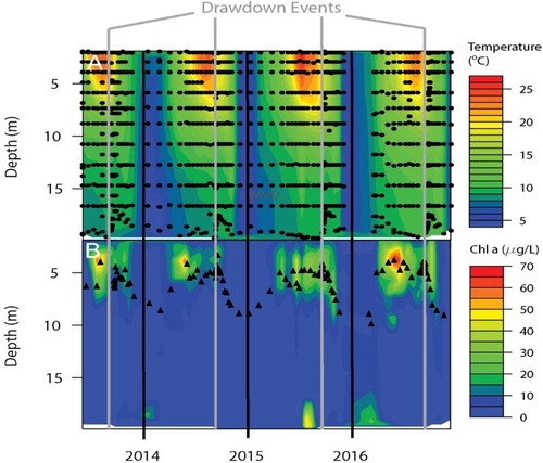
The concentration and vertical distribution of Chl-a measured by the Sonde showed a clear seasonal pattern, with the occurrence of 1 or more subsurface Chl-a maxima (SCM) of 30–60 µg/L at depths of 2–8 m during each late spring/early summer period (Figure 2(B)). However, the magnitude and extent of these SCM varied greatly between years. In 2013, a month-long SCM occurred in July-August, whereas in 2014 it occurred in May-June. There was also a prolonged period (March-October) of multiple, less intense (<40 µg/L) SCM in 2015. Similar prolonged, multiple SCM were also present in 2016, but in contrast to the other years, the Chl-a maxima were extremely high (60–70 µg/L), especially during spring and again briefly in autumn (Figure 2(B)). The weighted mean depths of Chl-a concentration calculated from the Sonde profiles generally followed the pattern of SCM depths, being shallower during the summer when Chl-a was higher and concentrated in the upper water column, and deeper during the winter months when Chl-a concentrations were relatively low and more uniformly distributed vertically (Figure 2(B)).

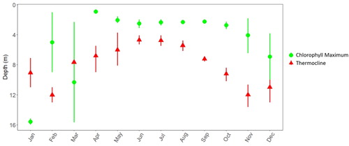
Averaging across our 4 years of data, a clear if unsurprising seasonal pattern is evident in the depth of the thermocline: initial development during spring, followed by strengthening and shoaling during summer, then erosion and water column turnover in autumn (Figure 3). Similarly, shoaling in spring and summer occurred in the depth of the Chl-a maxima, but there was less erosion and deepening of the SCM than in the thermocline later in the year. More specifically, the SCM usually occurred several meters above the thermocline during the summer, and it was consistently 6–8 m above the thermocline from September through November (Figure 3).

Figure 3. Monthly mean (± standard error) depth of the thermocline (red triangles) and the Chl-a maximum (green circles) during 2013–2016 in Lacamas Lake, Washington.

Drawdown of lake levels for dam maintenance occurred during a period of ∼2 weeks in September/October of each year (Figures 1 and 2); however, there were no obvious effects of the drawdown on the vertical distribution of either water temperature (Figure 2A) or Chl-a (Figure 2B). Moreover, for the 2 dates on which we collected replicated vertical profiles of size-fractionated Chl-a concentration (pre-drawdown: 20–21 August and post-drawdown: 17–18 October 2015), very similar patterns were observed across dates and across size fractions: Chl-a was generally limited to the upper mixed layer (0–10 m), and was usually most concentrated in the upper 5 m of the water column (Figure 4). Midday versus midnight vertical distributions were remarkably similar across all size classes, with only the 2.7–35 µm size fraction in October showing any significant diel difference between WMDs as assessed using t-tests (p = 0.0058, n = 3; Figure 4). There was also very little difference in vertical distribution of size-fractionated Chl-a between our August (pre-drawdown) and October (post-drawdown) sampling dates (Figure 4, Table 1). Although 3 of our 4 size fractions showed a statistically significantly deeper distribution in October (post-drawdown) than in August (pre-drawdown), this deepening was only ∼1 m (Figure 4, Table 1).

Figure 4. Vertical distributions of size-fractionated Chl-a concentrations in Lacamas Lake, Washington in (A) August, 2015 and (B) October 2015. Both midnight (black bars, left) and midday (gray bars, right) data are shown. The circles represent the mean weighted mean depth (WMD) for each size fraction. Of all the midday versus midnight comparisons, only the 2.7–35 µm size fraction in October showed any significant diel difference in mean WMDs (p = 0.0058, n = 3).

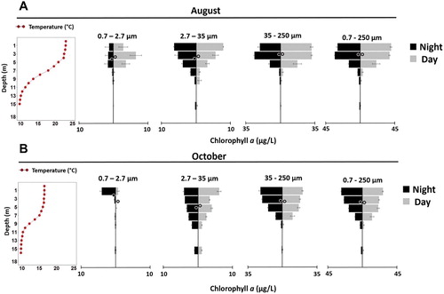
Table 1. Mean (± standard error) weighted mean depths (WMDs) in meters of each of 4 size fractions of Chl-a in August (pre-spill) and October (post-spill) 2015, and the difference in mean WMDs between the 2 dates, in Lacamas Lake, Washington, assessed using Student’s t-tests. (*** = p < 0.001, n = 6 [3 midday and 3 midnight samples were combined for each date]).

	0.7–2.7 µm	2.7–35 µm	35–250 µm	0.7–250 µm
20–21 August 2015	3.24 (0.69)	3.32 (0.12)	2.87 (0.10)	2.92 (0.10)
17–18 October 2015	2.69 (1.35)	4.66 (0.14)	3.49 (0.10)	3.73 (0.10)
Difference (October–August)	−0.55	1.34 ***	0.62 ***	0.81 ***

Discussion

The “seasonal deepening” of SCM throughout summer and into autumn was noted more than half a century ago (Steele 1956), and numerous times since (e.g. Longhurst 2007; Mignot et al. 2014; Lavigne et al. 2015). In the case of Lacamas Lake, however, we saw no such seasonal deepening. That is, the SCM consistently occurred at 2–5 m depth from June through October (Figures 2 and 3), with the mean vertical distance of the SCM above the thermocline increasing from June (2 m above) to November (6 m above) (Figure 3).

We did, however, see striking interannual variability in our temperature and Chl-a data. In 2015 the conditions were anomalously warm. These conditions occurred throughout much of the US Pacific Northwest (Mote et al. 2016), and are projected to become more common in coming decades (Rupp et al. 2017). Surface water temperatures in Lacamas Lake were highest during 2015, consistent with the regional patterns of air temperature, but the SCM was less pronounced in 2015 than in other study years. SCM Chl-a levels were highest in 2016, a cooler year. This result could have been due to a number of factors or processes (e.g., enhanced growth or reduced grazing) that we were unable to measure in this study. However these results suggest that temperature alone is not the primary driver of sub-surface Chl-a concentrations.

Although our study was focused on describing how Chl-a varies vertically in Lacamas Lake, why this variation might have occured is also of interest. Several previous studies shed light on this, and lead to the following insights and hypotheses about possible control mechanisms that build upon our observations and could be explored in future studies. First, within the very near surface layer (0–2 m) it is possible that photo-inhibition and/or grazing kept Chl-a low, as nutrients are generally high in Lacamas Lake (Deemer et al. 2011, 2015), with a typical temperate, freshwater assemblage of zooplankton grazers (Nolan et al., forthcoming). Second, during our study, conditions must have been favorable for phytoplankton (e.g., high growth and/or reduced grazing) to allow for the development and maintenance of persistently high Chl-a concentration within the SCM (∼2–5 m). Third, just below the SCM (6–10 m), grazing, but probably not nutrient limitation, was likely keeping Chl-a low during our study period (again, nutrients are generally high in the epilimnion of Lacamas Lake [Deemer et al. 2011, 2015] and zooplankton grazers often have peak abundances at 6–10 m (Nolan et al., forthcoming). Fourth, phytoplankton sinking, while likely occurring to some degree, did not result in build-up of Chl-a at the thermocline in our observations, as has been observed elsewhere (Cullen 2015 and references therein). Fifth, low Chl-a in the hypolimnion was probably the result of some combination of light limitation and grazing, as several zooplankton taxa inhabit the hypoxic hypolimnion of the reservoir (Nolan et al., forthcoming). Future studies of these phenomena will be needed to fully explain the dynamics underlying SCM in Lacamas Lake.

As for drawdown effects in this managed reservoir, in the one case where we collected replicate samples both before (August 2015) and after (October 2015) drawdown, we saw a very small (∼1 m) but nevertheless statistically significant deepening in Chl-a distribution. Sonde time-series data, which were not replicated and thus not amenable to statistical testing, also suggested only minimal effects (if any) of drawdown events on the vertical distribution of either temperature or Chl-a in Lacamas Lake. Indeed, both thermal stratification and (to a lesser degree) SCM persisted well into autumn, even after the occurrence of annual drawdown events. These results roughly align with observations of the effect of drawdown on SCM in the few other reservoirs where this has been examined. In the Pepacton Reservoir in New York, a distinct SCM at ∼10 m depth was observed during July, when the reservoir was at its greatest depth (∼45 m), and did not change as water was slowly drawn down to a reservoir depth of ∼30 m over the next 3 months (Effler and O’Donnell 2001). Similarly, Sevindik et al. (2017) observed relatively strong SCM in a Turkish reservoir, and reported nutrients and temperature to be more important than water removal in modulating phytoplankton dynamics.

The managed drawdown did not appear to affect diel differences in Chl-a vertical distributions. We observed almost no statistically significant diel differences in WMD of Chl-a, except in the 2.7–35 µm size fraction after drawdown, when midnight WMD was slightly (<0.5 m) deeper than at midday. Our observation of almost no diel vertical migration of phytoplankton contrasts to some degree with other studies that have reported diel vertical migration among some phytoplankton taxa (Reynolds 2006; deNoyelles et al. 2016). However, the drawdown of water in Lacamas Lake occurs from within the epilimnion (at ∼2 m depth). It is possible that other reservoirs where drawdown occurs within the deeper metalimnion or hypolimnion might exhibit different effects on temperature and Chl-a. It should be noted that the drawdown of water in Lacamas Lake occurs over a relatively short period of time (2–3 weeks) compared to many reservoirs, and the lake then refills naturally over the next 6–8 weeks concurrent with the beginning of the rainy season in the Pacific Northwest. This rather rapid refilling of the lake did not, however, appear to influence the vertical distribution of Chl-a.

In summary, our results suggest that in Lacamas Lake there is a very limited effect of drawdown on the vertical distribution of Chl-a generally and SCM specifically. This suggests the need for further investigation to identify the ecological and biogeochemical mechanisms underlying the heterogeneity of phytoplankton vertical distribution in managed reservoirs, and how these may be modulated by different reservoir drawdown practices.

Acknowledgments

We thank K. Birchfield, J. Zimmerman, and S. Nolan for assistance with field collections.

Additional information

Funding

This research was supported by a National Science Foundation (NSF) REU grant number 1461057 to G. Rollwagen-Bollens and S. Bollens, and US Army Corps of Engineers IWR, NSF ETBC grant number 1045286, and NSF DEB grant number 1355211 to J. Harrison.

References

- Abbott MR, Denman K, Powell TM, Richerson PJ, Richards RC, Goldman CR. 1984. Mixing and the dynamics of the deep chlorophyll maximum in Lake Tahoe. Limnol Oceanogr. 29(4):862–878.
- Alldredge AL, Cowles TJ, MacIntyre S, Rines JEB, Donaghay PL, Greenlaw CF, Holliday DV, Dekshenieks MM, Sullivan JM, Zaneveld JRV. 2002. Occurrence and mechanisms of formation of a dramatic thin layer of marine snow in a shallow Pacific fjord. Mar Ecol Prog Ser. 233:1–12.
- Barbiero RP, Tuchman ML. 2004. The deep chlorophyll maximum in lake superior. J Great Lakes Res. 30:256–268.
- Bienfang PK, Szyper JP, Okamoto MY, Noda EK. 1984. Temporal and spatial variability of phytoplankton in a subtropical ecosystem. Limnol Oceanogr. 29(3):527–539.
- Bochdansky AB, Bollens SM. 2009. Thin layer formation during runaway stratification in the tidally dynamic San Francisco Estuary. J Plankt Res. 31(11):1385–1390.
- Bollens SM, Osgood K, Frost BW, Watts SD. 1993. Vertical distributions and susceptibilities to vertebrate predation of the marine copepods Metridia lucens and Calanus pacificus. Limnol Oceanogr. 38(8):1827–1837.
- Chapin BRK, DeNoyelles F, Graham DW, Smith VH. 2004. A deep maximum of green sulphur bacteria (‘Chlorochromatium aggregatum’) in a strongly stratified reservoir. Freshwater Biol. 49(10):1337–1354.
- Cullen JJ. 2015. Subsurface chlorophyll maximum layers: enduring enigma or mystery solved? Ann Rev Mar Sci. 7:207–239.
- Deemer BR, Harrison JA, Li S, Beaulieu JJ, DelSontro T, Barros N, Bezerra-Neto JF, Powers SM, dos Santos MA, Vonk JA. 2016. Greenhouse gas emissions from reservoir water surfaces: A new global synthesis. BioScience. 66(11):949–964.
- Deemer BR, Harrison JA, Whitling EW. 2011. Microbial dinitrogen and nitrous oxide production in a small eutrophic reservoir: an in situ approach to quantifying hypolimnetic process rates. Limnol Oceanogr. 56(4):1189–1199.
- Deemer BR, Henderson SM, Harrison JA. 2015. Chemical mixing in the bottom boundary layer of a eutrophic reservoir: the effects of internal seiching on nitrogen dynamics: chemical mixing in the bottom boundary layer. Limnol Oceanogr. 60(5):1642–1655.
- deNoyelles F, Smith V, Kastens J, Bennett L, Lomas J, Knapp C, Bergin S, Dewey S, Chapin B, Graham D. 2016. A 21-year record of vertically migrating subepilimnetic populations of Cryptomonas spp. IW. 6(2):173–184.
- Effler SW, O’Donnell DM. 2001. Resolution of spatial patterns in three reservoirs with rapid profiling instrumentation. Hydrobiologia. 450(1/3):197–208.
- Harrison JA, Frings PJ, Beusen AHW, Conley DJ, McCrackin ML. 2012. Global importance, patterns, and controls of dissolved silica retention in lakes and reservoirs. Global Biogeochem Cy. 26:GB2037.
- Harrison JA, Maranger RJ, Alexander RB, Giblin AE, Jacinthe P-A, Mayorga E, Seitzinger SP, Sobota DJ, Wollheim WM. 2009. The regional and global significance of nitrogen removal in lakes and reservoirs. Biogeochemistry. 93(1–2):143–157.
- Lavigne H, D’Ortenzio F, Ribera D’Alcalà M, Claustre H, Sauzède R, Gacic M. 2015. On the vertical distribution of the chlorophyll a concentration in the Mediterranean Sea: a basin-scale and seasonal approach. Biogeosciences. 12(16):5021–5039.
- Leach TH, Beisner BE, Carey CC, Pernica P, Rose KC, Huot Y, Brentrup JA, Domaizon I, Grossart H-P, Ibelings BW, et al. 2018. Patterns and drivers of deep chlorophyll maxima structure in 100 lakes: The relative importance of light and thermal stratification: patterns and drivers of DCM structure across lakes. Limnol Oceanogr. 63(2):628–646.
- Lehner B, Liermann CR, Revenga C, Vörösmarty C, Fekete B, Crouzet P, Döll P, Endejan M, Frenken K, Magome J, et al. 2011. High-resolution mapping of the world’s reservoirs and dams for sustainable river-flow management. Front Ecol Env. 9(9):494–502.
- Longhurst AR. (ed.). 2007. Preface. In: Ecological geography of the sea. 2nd ed. Burlington (MA): Academic Press; p. xi–xiii.
- Martin J, Tremblay J, Gagnon J, Tremblay G, Lapoussière A, Jose C, Poulin M, Gosselin M, Gratton Y, Michel C. 2010. Prevalence, structure and properties of subsurface chlorophyll maxima in Canadian Arctic waters. Mar Ecol Prog Ser. 412:69–84.
- Menden-Deuer S. 2008. Spatial and temporal characteristics of plankton-rich layers in a shallow, temperate fjord. Mar Ecol Prog Ser. 355:21–30.
- Mignot A, Claustre H, Uitz J, Poteau A, D'Ortenzio F, Xing X. 2014. Understanding the seasonal dynamics of phytoplankton biomass and the deep chlorophyll maximum in oligotrophic environments: a bio-argo float investigation. Global Biogeochem Cycles. 28(8):856–876.
- Mineeva NM, Mukhutdinov VF. 2018. Vertical distribution of chlorophyll in the upper volga reservoirs. Inland Water Biol. 11(1):13–20.
- Mote PW, Rupp DE, Li S, Sharp DJ, Otto F, Uhe PF, Xiao M, Lettenmaier DP, Cullen H, Allen MR. 2016. Perspectives on the causes of exceptionally low 2015 snowpack in the western United States: Low Snowpack in 2015 in the Western U.S. Geophys Res Lett. 43(20):10980–10988.
- Nolan S, Bollens S, Rollwagen-Bollens G. Forthcoming. Diverse taxa of zooplankton inhabit hypoxic waters during both day and night in a temperate eutrophic lake. J Plankt Res.
- Paerl H. 2008. Chapter 10. Nutrient and other environmental controls of harmful cyanobacterial blooms along the freshwater–marine continuum. Adv Exp Med Biol. 619:217–237.
- Paerl HW, Otten TG. 2013. Harmful cyanobacterial blooms: causes, consequences, and controls. Microb Ecol. 65(4):995–1010.
- Reynolds CS. 2006. The ecology of phytoplankton. Cambridge (UK): Cambridge University Press.
- Rupp DE, Abatzoglou JT, Mote PW. 2017. Projections of 21st century climate of the Columbia River Basin. Clim Dyn. 49(5–6):1783–1799.
- Sevindik TO, Çelik K, Naselli-Flores L. 2017. Spatial heterogeneity and seasonal succession of phytoplankton functional groups along the vertical gradient in a mesotrophic reservoir. Ann Limnol. 53:129–141.
- Steele JH. 1956. Plant production on the Fladen ground. J Mar Biol Ass. 35(1):1–33.
- Strickland J, Parsons T. 1972. A practical handbook for seawater analysis. Fisheries Research Board of Canada Bulletin.
- Zarfl C, Lumsdon AE, Berlekamp J, Tydecks L, Tockner K. 2015. A global boom in hydropower dam construction. Aquat Sci. 77(1):161–170.