To measure chlorophyll or phytoplankton biovolume: an aquatic conundrum with implications for the management of lakes

Abstract

Canfield DE, Jr., Bachmann RW, Hoyer MV, Johansson LS, Søndergaard M, and Jeppesen E. 2018. To measure chlorophyl or phytoplankton biovolume: an aquatic conundrum with implications for the management of lakes. Lake Reserv Manage. 35:181–192.

The log₁₀-transformed relationship between measured phytoplankton biovolumes and chlorophyll concentrations, surrogates for algal biomass, was examined using 13,000-plus paired samples collected from lakes in Denmark (250), the continental United States (1835), and Florida (159). A positive (R² = 0.57) relationship was found but predicted biovolumes had a 95% confidence interval of 11–912%. Regressing chlorophyll as opposed to phytoplankton biovolume against total phosphorus (TP) (R² = 0.43 vs. R² = 0.21), total nitrogen (TN) (R² = 0.24 vs. R² = 0.08), and Secchi disk (SD) (R² = 0.60 vs. R² = 0.39) yielded stronger relationships. Three algal groups (Cyanophyta, Chlorophyta, and Bacillariophyceae) contributed approximately 100% of the biovolume in some samples. For these groups and samples, biovolume increased significantly with chlorophyll (R² = 0.35, R² = 0.27, and R² = 0.31, respectively) and TP (R² = 0.18, R² = 0.13, and R² = 0.13) and decreased significantly with increases in SD (R² = 0.29, R² = 0.31, and R² = 0.17). All empirical relationships had substantial confidence intervals. Contingency tables for variance within the independent (horizontal variance) and dependent (vertical variance) variables are presented, providing managers information on how much change is required to insure noticeable effects. If resources are limited, chlorophyll is recommended for monitoring long-term trends because it provides an estimate of biomass magnitude and has better relationships with nutrients and SD. Managers may integrate occasional biovolume measurements if concerned with Cyanophyta abundance, taste and odor production, or changing algal population dynamics.

Keywords:

• Algal biomass
• chlorophyll
• nutrients
• Secchi
• contingency tables

Publication of chlorophyll–phosphorus relationships (Dillon and Rigler 1974; Jones and Bachmann 1976) and the Carlson (1977) Trophic State Index (TSI) provided impetus for members of the research, regulatory, and lake management communities to use chlorophyll (Chl) measurements as a surrogate for phytoplankton biomass. Chl has become a measurement of choice because it is a relatively inexpensive chemical method, many samples can be analyzed in a short period of time, and most laboratories can perform the test. Estimating phytoplankton biovolumes (i.e., biomass) and species composition, however, remains an important issue for many professionals (Carvalho et al. 2012; Richardson et al. 2018) because many managers have concerns about taste and odor problems, Cyanophyta toxins, or changing algal population dynamics (Carmichael 2001; Downing et al. 2001; Pick 2016). However, microscopic determinations of phytoplankton biovolume are time-consuming and costly, require individuals with algal taxonomic expertise, and comparable results are often difficult to obtain because there are different approaches for calculating biovolumes for different species (Hillebrand et al. 1999).

Managers are therefore faced with a conundrum of whether to measure Chl or total phytoplankton biovolume, especially because it is recognized that Chl is not an accurate measure of phytoplankton biomass (Canfield et al. 1985; Kasprzak et al. 2008; Ramaraj et al. 2013). In this article we use more than 13,000 individual lake-water samples to determine how well concurrent measurements of Chl concentrations and microscopic-determined phytoplankton biovolumes are associated, what is the magnitude of the uncertainties associated with biovolume predictions from Chl, and which of these two measures of algal abundance are more closely related to trophic state indicators (i.e., total phosphorus [TP], total nitrogen [TN], and Secchi disk [SD]). We also examine how the biomass compositions of the three dominant algal groups (Cyanophyta, Chlorophyta, and Bacillariophyceae) are related to the trophic state indicators. Finally, we discuss management implications because of the large errors associated with empirical predictions due to both the variance associated with the independent (horizontal variance) and dependent (vertical variance) variables of many of the important bivariate limnological relationships used for the management of aquatic systems.

Materials and methods

Concurrently measured total phytoplankton biovolume (mm³/L), Chl, nutrients (TP and TN), and Secchi disk (SD) data from 159 Florida lakes (Canfield et al. 1985), 250 lakes from the Danish National Monitoring Program (Kronvang et al. 1993), and 1835 U.S. lakes sampled by the U.S. Environmental Protection Agency during their 2007/2012 National Lake Assessment (NLA) surveys (USEPA 2009, 2016) were retrieved. Florida provided 318 individual samples, Denmark provided 10,658 samples, and the NLA yielded 2187 samples (see supplement for additional information).

Many investigators aggregate data by averaging samples for individual water bodies, but minimizing aggregation was considered important because there can be unexpected negative effects of data aggregation regression model predictability (Jones et al. 1998). Our interest was also the environmental conditions that existed when each sample was collected, and the assembled data represented a wide range of limnological and phytoplankton community conditions (Tables 1 and 2; also in supplemental information). Both the Danish (Kronvang et al. 1993) and the NLA (USEPA 2012) data also underwent rigorous national quality assurance/quality control examinations, whereas the Florida data did not undergo such stringent examinations (Canfield et al. 1985). However, pooling the data raised a concern that analyses would be influenced greatly by the Danish database. Thus, data from Florida, Denmark, and the NLA were independently randomized and 200 samples from each group were extracted to provide a balanced, pooled database of 600 samples (SAS 2000). The 600-sample database also represented a wide range of limnological and phytoplankton community conditions (Tables 1 and 2; also in supplemental information).

Table 1. Frequency distributions of trophic state parameters and temperature measured in individual water samples collected from Denmark (N = 10,658), Florida (N = 318), and during the U.S. Environmental Protection Agency’s (USEPA) National Lake Assessment (NLA) surveys (N = 2187). Numbers in parentheses are values from a randomized database where 200 samples each were taken from Denmark, Florida, and the NLA.

Variable	Minimum	25% Quantile	Mean	Median	75% Quantile	Maximum
Denmark
Chlorophyll (µg/L)	0.2 (0.9)	9 (7)	59 (63)	27 (28)	72 (83)	1100 (650)
Total P (µg/L)	2 (7)	50 (56)	167 (165)	96 (100)	200 (200)	2990 (2300)
Total N (µg/L)	33 (340)	960 (940)	2268 (760)	1600 (570)	2821 (930)	22,000 (6100)
Secchi (m)	0.1 (0.2)	0.7 (0.6)	1.7 (1.6)	1.3 (1.2)	2.2 (2.3)	11 (6.5)
Florida
Chlorophyll (µg/L)	0.3 (0.3)	3 (3)	18 (17)	5 (5)	17 (17)	311 (311)
Total P (µg/L)	1 (1)	11 (11)	50 (49)	21 (21)	43 (43)	1090 (1090)
Total N (µg/L)	65 (65)	370 (380)	780 (760)	560 (570)	950 (930)	6100 (6100)
Secchi (m)	0.1 (0.1)	0.6 (0.6)	1.8 (1.7)	1.2 (1.2)	2.4 (2.2)	9 (9)
USEPA NLA
Chlorophyll (µg/L)	<1 (<1)	3 (3)	28 (31)	8 (9)	26 (33)	940 (274)
Total P (µg/L)	1 (1)	14 (14)	115 (142)	35 (37)	95 (120)	4680 (3600)
Total N (µg/L)	5 (33)	320 (320)	1200 (1300)	610 (680)	1230 (1430)	54,000 (17000)
Secchi (m)	<0.1 (<0.1)	0.6 (0.6)	2.1 (2.1)	1.4 (1.2)	2.8 (2.6)	37 (28)

Table 2. Frequency distributions of phytoplankton groups measured concurrently with chemical and physical limnological state parameters in individual water samples collected from Denmark (N = 10,658), Florida (N = 318) and during the U.S. Environmental Protection Agency’s National Lake Assessment survey (N = 2,187). Numbers in parentheses are values from a randomized database where 200 samples each were taken from Denmark, Florida, and the NLA.

Total Biovolume (mm^3/L)
Phytoplankton Groups	Minimum	25% Quantile	Mean	Median	75% Quantile	Maximum
Denmark
Total	0.0 (<0.1)	1.1 (1.1)	10 (10)	4 (4)	11 (11)	1100 (110)
Cyanophyta	0.0 (0.0)	0.0 (0.0)	4 (4)	0.0 (0.1)	2 (3)	480 (110)
Chlorophyta	0.0 (0.0)	0.0 (<0.1)	2 (2)	0.1 (0.1)	0.9 (1)	1000 (51)
Diatom	0.0 (0.0)	0.0 (0.0)	2.0 (1.7)	0.1 (0.1)	1.2 (1.1)	177 (51)
Cryptophyta	0.0 (<0.1)	0.1 (0.1)	0.5 (0.7)	0.2 (0.2)	0.5 (0.7)	28 (11)
Dinoflagellate	0.0 (0.0)	0.0 (0.0)	0.9 (0.5)	0.0 (0.0)	0.1 (0.1)	234 (25)
Euglenoid	0.0 (0.0)	0.0 (0.0)	0.0 (<0.1)	0.0 (0.0)	0.0 (0.0)	31 (3)
Chrysophyta	0.0 (0.0)	0.0 (0.0)	0.0 (0.1)	0.0 (0.0)	0.0 (0.0)	5 (0.4)
Xanthophyta	0.0 (0.0)	0.0 (0.0)	0.0 (0.0)	0.0 (0.0)	0.0 (0.0)	4 (0.0)
Florida
Total	0.0 (0.1)	1 (1)	40 (45)	2 (3)	13 (14)	2900 (2900)
Cyanophyta	0.0 (0.0)	0.0 (0.0)	35 (40)	0.2 (0.3)	5 (6)	2900 (2900)
Chlorophyta	0.0 (0.0)	0.1 (0.1)	2 (2)	0.3 (0.3)	1.3 (1.4)	130 (35)
Diatom	0.0 (0.0)	0.0 (<0.1)	1.7 (1.7)	0.3 (0.3)	1.4 (1.6)	39 (39)
Cryptophyta	0.0 (<0.1)	0.0 (<0.1)	0.2 (0.2)	0.1 (0.1)	0.2 (0.2)	15 (3)
Dinoflagellate	0.0 (0.0)	0.0 (0.0)	0.3 (0.3)	<0.1 (<0.1)	0.2 (0.2)	11 (11)
Euglenoid	0.0 (0.0)	0.0 (0.0)	0.0 (<0.1)	0.0 (0.0)	0.0 (0.0)	3 (0.3)
Chrysophyta	0.0 (0.0)	0.0 (0.0)	0.0 (<0.1)	0.0 (0.0)	0.0 (0.0)	0.7 (0.2)
Xanthophyta	0.0 (0.0)	0.0 (0.0)	0.1 (0.1)	0 (0.0)	0.0 (0.0)	3 (3)
USEPA NLA
Total	0.0 (<0.1)	1 (1)	12 (20)	3 (4)	8 (16)	1300 (1300)
Cyanophyta	0.0 (0.0)	0.1 (0.1)	4 (5)	0.3 (0.3)	1 (2)	4309 (94)
Chlorophyta	0.0 (0.0)	0.0 (<0.1)	3 10	0.2 (0.3)	1.1 (1.3)	1310 (1310)
Diatom	0.0 (0.0)	0.0 (<0.1)	1.4 (1.3)	0.1 (0.1)	0.5 (0.7)	204 (32)
Cryptophyta	0.0 (<0.1)	0.0 (<0.1)	0.9 (1)	0.1 (0.1)	0.5 (0.5)	131 (48)
Dinoflagellate	0.0 (0.0)	0.0 (0.0)	2.1 (2.4)	0.0 (0.1)	1.0 (1.4)	436 (120)
Euglenoid	0.0 (0.0)	0.0 (0.0)	0.0 (0.7)	0.0 (0.0)	0.1 (0.1)	51 (43)
Chrysophyta	0.0 (0.0)	0.0 (0.0)	0.2 (0.1)	0.0 (0.0)	0.0 (0.0)	230 (6)
Xanthophyta	0.0 (0.0)	0.0 (0.0)	0.0 (<0.1)	0 (0.0)	0.0 (0.0)	2 (0.1)

When data were plotted, there were some notable outliers from the Danish and NLA datasets, but none from the Florida dataset. Outliers were examined and obvious errors eliminated, but no further judgment was made on the quality of the remaining data (see supplemental information for criteria used to remove data). Because the data ranged considerably and variances were proportional to the mean values, all data were log₁₀-transformed prior to statistical analyses (Sokal and Rohlf 1981). Although there are many ways to transform data, the log₁₀ transformation was chosen because such transformed data are routinely reported in applied management articles.

In searching for patterns among the phytoplankton biovolume data and potential correlates, we used ordinary least-squares regression (OLSR). Regression analyses, however, estimate the conditional means of the response variables for different correlate values, and potential problems exist between the underlying statistical assumptions and the ecological concept of limiting factors (Kaiser et al. 1994). Consequently, there is often an effort to identify a “factor ceiling” to the data distribution rather than focusing on just the mean response of the dependent variable (Thomson et al. 1996; Brown et al. 2000; Jones et al. 2011). A “factor ceiling” is identified as the upper boundary response of the dependent variable across the entire range of the independent variable and it is assumed the boundary represents the point where the independent variable is the probable limiting environmental factor.

Carlson (1977), recognizing the tremendous variability that trophic variables exhibit in lakes, developed a scale of 0 to 100, the Trophic State Index (TSI), for Chl, TP, and SD, assuming TP was the limiting nutrient. Each TSI division (10, 20, 30, etc.) represented a doubling in algal biomass. Kratzer and Brezonik (1981) developed a TN TSI for nitrogen-limited Florida lakes. Although TSIs have found widespread use in lake management, the indices were developed using small databases. Rather than redeveloping the TSIs with our large database, the continuums of examined limnological variables were divided into 10 deciles. This aggregation of data resulted in each decile grouping having over 1000 samples with the lower and upper boundaries (Table 3 in supplemental information) for the examined variables (Chl, total phytoplankton biovolume, TP, TN, and SD).

All statistics were obtained by use of JMP software (SAS 2000). Decile means were compared using the Tukey HSD (Tukey–Kramer) to determine significant differences. Within each decile, histograms were constructed to visually illustrate the vertical distribution of the dependent variable. When OLSR was used to investigate bivariate relationships, the root mean square error (RMSE) was used to calculate a 95% confidence interval (CI) for predicted values. Because the data were log₁₀-transformed, the CI values were expressed as percentages. The upper bound was calculated as 100 × 10^(2×RMSE) and the lower bound was calculated as 100/10^(2xRMSE). A significance level of p ≤ 0.05 was used for all statistical tests.

To further address the importance of vertical variance within the examined dependent variables (Chl and total phytoplankton biovolumes) and horizontal variance within the independent variables (TP, TN, and SD), we created contingency tables (JMP 2000). Within the contingency box, the percent of samples expected to fall within that box was provided for the purpose of deciding how much change in the independent variable would be needed to accomplish a desired level of change in the dependent variable and what are the chance of having higher or lower values, providing managers with information on the chance of having an algal bloom or a clearing event.

Results and discussion

Predicting total phytoplankton biovolume

An important question for lake managers is how well Chl measurements can predict phytoplankton biovolumes (i.e., biomass) determined by microscopic examinations. Using the log₁₀-transformed data (13,147 pairs), there was a statistically significant positive-linear relationship (Figure 1) but the R² was 0.57 and the RMSE was 0.48. For this RMSE, the 95% CI for a predicted biovolume value would be 11% to 912%, raising the question of whether this linear regression, although statistically significant, would be useful for most lake managers (Prairie 1996; Bryhn and Dimberg 2011).

Figure 1. Plots and regression equations for log₁₀-transformed total phytoplankton biovolume (mm³/L) versus log₁₀-transformed chlorophyll (µg/L) for all data and by location using paired samples from Denmark (N = 10,658), Florida (N = 318), and during the U.S. Environmental Protection Agency’s National Lake Assessment survey (N = 2187).

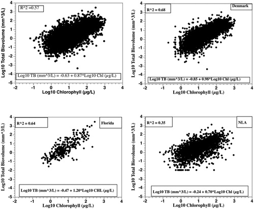
Since the 1970s, considerable effort has been expended both regionally and globally to refine/improve empirical Chl–nutrient models (Brown et al. 2000; Abell et al. 2012; Xu et al. 2015). Abell et al. (2012) provided evidence that there was latitudinal variation in Chl–nutrient relationships in lakes, suggesting location might be a major factor contributing to the observed variance in phytoplankton biovolumes. In our study, Danish samples were from lakes located above 55°N and Florida samples were from lakes below 30°N. Both Denmark (R² = 0.68) and Florida (R² = 0.64) exhibited stronger phytoplankton biovolume–Chl relationships than the whole dataset (Figure 1), but both regressions also had substantial 95% CIs (16–630% for Denmark and 8–1200% for Florida).

The randomized 600-sample database provided similar results for all data (R² = 0.47, RMSE = 0.59), Denmark (R² = 0.65, RMSE = 0.44), Florida (R² = 0.61, RMSE = 0.56), and the NLA (R² = 0.47, RMSE = 0.59), again indicating the large CIs are not just only the result of location. An effect of location cannot be totally ruled out as the coefficients of variance for log₁₀-phytoplankton biovolume were 133% for Denmark, 177% for Florida, and 184% for the NLA.

Most managers, however, focus on one lake or a few lakes located in a limited geographical area. There were 35 Danish lakes with 10 to 23 yr of monthly (Jan to Dec) measurements (number of samples per month: 1 to 23). When regressing log₁₀-total phytoplankton biovolumes against log₁₀-Chl concentrations, 15 of 35 lakes had R² > 0.65 with the best R² = 0.85. The RMSE for the best lake was 0.26, resulting in a 95% CI of 30% to 331%. For the other 20 lakes, RMSEs were >0.30 (0.31 to 0.53). Kasprzak et al. (2008) concluded that caution is warranted whenever Chl would be used to predict microscopically determined phytoplankton biovolumes.

The intense recreational-use summer months (July, August, and sometimes September) garner the attention of many northern hemisphere researchers and managers. Many Chl–nutrient models, therefore, focus on predicting summer Chl concentrations (Jones and Bachmann 1976; Søndergaard et al. 2016). Our database contained 4271 July/August pairs of total phytoplankton biovolume and Chl measurements. Sampling in September was limited or not done (Florida) so September data were not used. The randomized database contained 274 July/August pairs. There were statistically significant positive-linear relationships for the entire database (R² = 0.55, RMSE = 0.50) and the randomized database (R² = 0.45, RMSE = 0.62). Examining the potential effect of location with the July/August data, Denmark (R² = 0.64, RMSE = 0.38) and Florida (R² = 0.61, RMSE = 0.58) again had stronger phytoplankton biovolume–Chl relationships than the NLA, but the 95% CIs were substantial (17–580% for Denmark, 7–1400% for Florida). For the randomized database, relationships were weaker (Denmark: R² = 0.57, RMSE = 0.56; Florida: R² = 0.54, RMSE = 0.61) and CIs remained large.

Danish and Florida samples came from lakes that the investigators chose to study for different reasons. NLA samples were obtained from U.S. lakes selected by use of a probabilistic sampling regime; thus, NLA lakes covered a larger latitude gradient. The phytoplankton biovolume–Chl relationship (Figure 1) was weaker (R² = 0.35) than those developed for Denmark and Florida and the 95% CI was 6–1800% due to a RMSE of 0.63. Restricting analyses to the NLA’s July/August samples, the phytoplankton biovolume–Chl relationship gave an R² of 0.47 (RMSE = 0.61) and the CI was 6–1700%. The NLA data thus raise the question of how much of the observed variance is due to natural factors when the Danish and Florida studies with less variance are based on nonprobabilistic or nonrandomized sampling. Florida data also were not extensively quality assured, or quality controlled like the Danish and NLA studies (Kronvang et al. 1993; USEPA 2012).

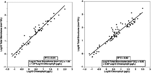
Given that there are a number of physical, chemical, and biological factors that could influence biovolume estimates per unit Chl, we attempted to identify a “factor ceiling” for the data distribution of the entire database (Figure 2) by using the JMP lasso function to arbitrarily extract the upper 55 points from the plotted total phytoplankton biovolume–Chl relationship (Figure 1) and 79 upper July/August data pairs. Both approaches (Figure 2) resulted in the development of statistically significant linear regressions with R² values >0.90 and RMSE values <0.25. The 95% CIs for the predicted values were 36–275% (all data) and 33–300% (July/August), so there were still large uncertainties involved in predicting phytoplankton biovolumes from Chl.

Figure 2. Plots and regression equations for log₁₀-transformed data points along the upper continuum of the total phytoplankton biovolume (mm³/L)–chlorophyll (µg/L) relationship for all data (left) and July/August data (right) for paired samples from Denmark (N = 10,658), Florida (N = 318), and during the U.S. Environmental Protection Agency’s National Lake Assessment survey (N = 2187).

Another approach for dealing with variance along the independent axis of the variables (i.e., Chl, TP, TN, and SD) of interest (horizontal variance) is to aggregate data into decile groupings. Within each horizontal decile, percentiles of the phytoplankton biovolumes (i.e., 10%, 25%, 50%, 75%, and 90% of the samples) can then be calculated to provide information on the distribution of the dependent variable (vertical variance). OLSR with each total biovolume percentile grouping can then be used to provide managers with equations that can be used to predict the vertical variance with changes in the horizontal deciles (Table 4 in supplemental information). With this type of data aggregation, OSLRs with R² values >0.90 and RMSE values <0.10 were developed for the larger database (similar results for the randomized database), with the exception being TN (R² values between 0.32 and 0.85 and RMSE between 0.11 and 0.24). All the regressions, however, still had large 95% CIs for predicted total phytoplankton biovolumes so caution is still warranted when trying to make predictions (Table 4 in supplemental information).

Trophic state indicators, chlorophyll, and phytoplankton biovolume relationships

Many managers are interested in monitoring a shift in lake trophic status. Using the entire dataset assembled, regressing log₁₀-Chl against log₁₀-TP (R² = 0.43) or log₁₀-TN (R² = 0.27) yielded greater R² values than using log₁₀-phytoplankton biovolume against log₁₀-TP (R² = 0.21) or log₁₀-TN (R² = 0.08). Log₁₀-Secchi against log₁₀-Chl (R² = 0.60) provided a much stronger relationship than using log₁₀-phytoplankton biovolume (R² = 0.39). For the Danish lakes with 10 or more years of sampling, only one lake out of the 35 studied had better relationships using log₁₀-total phytoplankton biovolume as the dependent variable. These findings provide an excellent basis for recommending the continued use of Chl measurements as the designated proxy for phytoplankton biomass. The empirical relationships, however, must be used cautiously due to variance caused by other limiting environmental factors.

Phytoplankton composition

There are patterns with phytoplankton biovolume estimates and changes in Chl, TP, TN, and SD expressed as deciles (Figure 1 in supplemental information). What type of algae are in the water, however, is always a question that emerges when water clarity is reduced due to an algal bloom. Total phytoplankton biovolumes were dominated by three algal groups: the Cyanophyta, Chlorophyta, and Bacillariophyceae, with minor contributions (not discussed here) from other groups (dinoflagellates, euglenoids, chrysophytes, cryptophytes, and xanthophytes: Table 2 in supplemental information). The average percent contribution of the Cyanophyta increased with changes in Chl (expressed as deciles) from approximately 25% when Chl was <14 µg/L to more than 40% when Chl exceeded 51 µg/L (Figure 2 of the supplemental information). Average Chlorophyta percent contributions, however, were greatest at Chl decile-10 (25%) and decile-99 (31%), and Bacillariophyceae percent contributions did not change significantly with increases with Chl.

There were samples where the three dominant groups did not contribute to the measured biovolume, but there were samples (Cyanophyta, N = 131; Chlorophyta, N = 32; Bacillariophyceae, N = 39) where a group contributed 100% of the measured biovolume. When these groups represent 100% of the sample, there were statistically significant positive-linear relationships between total Cyanophyta, Chlorophyta, and Bacillariophyceae biovolumes and Chl concentrations, but the R² values were < 0.40 (Cyanophyta 0.35, Chlorophyta 0.27, Bacillariophyceae 0.30). RMSEs were >0.8; thus, the 95% CIs for each group were substantial (Cyanophyta 2—5500%, Chlorophyta 2—4200%, Bacillariophyceae 3—3200%). Regressing the individual algal group’s biovolumes against TP (R² from 0.12 to 0.18) and TN (R² from 0.03 and 0.09) also yielded statistically significant positive-linear relationships. Using the criteria (R² > 0.65) of Prairie (1996) and Bryhn and Dimberg (2011), the relationships for applied managers are “statistically meaningless” and are only significant because of the large sample size (8000+ samples).

Light is another environmental factor that can influence algal populations. Using SD measurements as a proxy for light conditions, the percent contribution of Cyanophyta and Chlorophyta declined significantly as water got clearer (Figure 3 in supplemental information). Both algal groups had their greatest percent contribution when SD readings were <0.6 m (Secchi deciles 10 and 20). The Bacillariophyceae, however, did not change significantly with changes in water clarity, with the exception that the percent contribution of Bacillariophyceae was significantly less when SD values were <0.4 m. Regressions for the three dominant algal biovolumes against SD again yielded significant negative relationships with substantial 95% CIs (Cyanophyta 2—6600%, Chlorophyta 3—3800%, Bacillariophyceae 2—4200%).

Phytoplankton biovolume/chlorophyll ratios

Chl content per unit of phytoplankton biomass decreases as algal standing stocks increase, and some of the factors responsible for this relationship have included phytoplankton community structure, temperature, and lake trophic status (Kasprzak et al. 2008). The average phytoplankton biovolume/Chl ratio for Florida was 1.18, 0.86 for NLA lakes, and 0.23 for Danish waters (Table 5 in supplemental information). Because of the large (13,000+) sample size, these ratios were significantly different between locations, but ratio values overlapped considerably. When Cyanophyta, Chlorophyta, or Bacillariophyceae composed 100% of the measured algal biomass (Table 6 in supplemental information), Cyanophyta had the greatest biovolume/Chl ratio, followed by the Bacillariophyceae and then the Chlorophyta. Variability of the biovolume/Chl ratio within any specific phytoplankton group ranged orders of magnitude, suggesting the ratios probably would have low value for most applied situations.

Using simple linear regression for Danish lakes with 10 or more years of sampling, annual average biovolume/Chl ratios did not change in 26 lakes, declined in 3 lakes, and increased significantly in 6 lakes. All the waterbodies with significant regressions had R² < 0.65, so these relationships were also weak. Multiple regressions using all the data with TP, TN, and SD as the independent variables and biovolume/Chl ratios as the dependent variable demonstrated 12 of the lakes had nonsignificant regressions. SD (14 lakes) and TN (12 lakes) had significant effects, but R² values were very small and the regressions were only significant because of large sample sizes.

Implications for lake management

Managers will inevitably be faced with the decision of whether to measure Chl or phytoplankton biovolumes. Both measures are only surrogates for phytoplankton biomass. We recommend that managers should not use Chl to predict phytoplankton biomass. If used, it must be used cautiously (Figure 1 in Kasprzak et al. 2008). More importantly, it should not be assumed that microscopic determinations of algal biomass are the “gold standard” because there are many uncertainties in the calculation and interpretation of biovolumes (Hillebrand et al.1999; Patrick Center for Environmental Studies; http://Bacillariophyceae.ansp.org/nawqa/biovol2001.aspx). While new technologies (e.g., imaging particle analysis) are being developed (Camoying and Yñiguez 2016), the equipment is expensive and laborious and the phytoplankton categories that can be discriminated are few compared to the outputs of microscopy. Managers recognizing their financial limitations will therefore have to clearly define their objectives before choosing to use Chl, microscopy, or new technologies.

Variance is the “bane of existence” for lake managers, for it is when extreme events like algal blooms occur that complaints regarding the “health” of the system multiply. Empirical models developed from multilake studies have advanced our limnological understanding of lake functioning. However, the best empirical TP (Canfield and Bachmann 1981) and TN (Bachmann 1980) loading models when tested had 95% CIs of 31–288% and 36–315%, respectively. When predicting Chl concentrations, 95% CIs ranged from 29–319% (the best) to 16–916% (Canfield 1983) and Secchi depths CIs ranged from 36–250% (the best) to 58–398% (Canfield and Hodgson 1983). Although human error and sampling variability are incorporated in the models, the empirical models reflect natural variability.

Managers reporting large CIs to the public, policymakers, or the entities that fund projects will certainly be asked whether the relationships are really useful. Prairie (1996) and Bryhn and Dimberg (2011) provided information (e.g., R² < 0.65) for determining which statistically significant models should be classified as “statistically meaningless.” Relationships would only become statistically meaningful to user groups, policymakers, and funding entities if management activities accomplished large environmental changes due to natural variability. The question then becomes how the manager communicates variance to these groups. One approach is to use TSI indices (Carlson 1977), but another approach for the manager is to use the contingency tables developed here (Table 7 in supplemental information). The advantage for managers is that they no longer need to rely only on the mean response provided by regression equations.

Contingency tables provide interested parties an insight into the variances associated with the independent (horizontal variance) and dependent (vertical variance) variables of different limnological relationships. Being unaware of horizontal and vertical variances can lead to the implementation of management programs where changes cannot be demonstrated or to perceptions that the program failed. For example (Table 7 in supplemental information), if the management goal was to achieve a TP of 10 µg/L (i.e., the TP 10 decile) most (72%) Chl measurements should fall into Chl decile-10 and decile-20 (Chl < 1 µg/L to 6 µg/L), but there is a 1% chance that a sample in Chl decile-60 (Chl 22 to 33 µg/L) could occur, an algal bloom. If nonprofessionals view an algal bloom as evidence that the “health” of the lake is compromised, they could deem the management program as failed even though the bloom may just be a natural occurrence. If measured Chl concentrations were between 79 and 136 µg/L, 90% of measured samples would be in TP decile-60 or greater. Only by getting TP reduced to <30 µg/L (TP decile-20) could a manager insure such elevated Chl concentrations would not be measured. For TP deciles 30, 40, and 50, the chance of measuring Chl > 79 µg/L falls to <6%, but there is also a chance (5–9%) of measuring a Chl < 6 µg/L, an extreme clearing event. Clearing events are remembered by the public and such events often become a nonachievable goal.

The importance of our findings may also explain why studies of lakes with more than 20 yr of data have shown that water clarity is not exhibiting downward trends or Chl upward trends despite changes in external loading (Lottig et al. 2014; Canfield et al. 2016, 2018). Although there are examples from Europe and elsewhere with clear responses (Jeppesen et al. 2005, 2007), natural variation and lake resiliency may help explain why Bachmann et al. (2013) found that the proportions of lakes categorized as oligotrophic, mesotrophic, eutrophic, and hypereutrophic for the presettlement time period in the United States were not significantly different from the proportions found in 2007 despite significant land-use changes and population growth. The Bachmann et al. findings challenged “conventional wisdoms” and now are the subject of scientific discussion (McDonald et al. 2014; Smith et al. 2014; Bachmann et al. 2014).

Since the 1970s, the focus of many lake management programs, if not most, has been a reduction of algal biomass through nutrient control, especially phosphorus. While phosphorus is important, most lake users focus on water clarity as an indicator of the “quality or health” of a water body. Increased water clarity also corresponds to higher lakefront property values (Boyle et al. 1999). Water clarity, however, is largely determined by inorganic solids (Hoyer and Jones 1983; Lind 1986), organic color (Brezonik 1978; Canfield and Hodgson 1983), and Chl (Bachmann et al. 2017), collectively called turbidity. In the USEPA’s NLA data, the Secchi transparency–turbidity relationships for natural lakes (R² = 0.85) and artificial lakes (R² = 0.86) were among the strongest empirical relationships (Bachmann et al. 2017). Combining the natural and artificial lake data yields an R² of 0.83 and RMSE of 0.19 with a 95% CI of 42–240%. This evidence suggests managers would be well served by measuring organic color, Chl, and turbidity in order to ascertain why water clarity is changing.

Conclusions

Researchers still have not resolved the “paradox of the plankton” (Hutchinson 1961), but there is an innate human desire to know what types of algae are in the water and now to what extent toxic algae are dominating. The benefit of algal counting is that one gets information on changes in species composition and overall changes in algal composition, which is of relevance (Nixdorf et al. 2008) for identifying the ecological status of lakes as requested in the European Water Framework Directive (WFD). In the WFD the status is evaluated against a reference conditions for each lake so that naturally turbid lakes would be judged in good ecological status and needing no improvement. This approach avoids the dilemma between choosing Chl or total algal biovolume, as both are relevant. Moreover, algal counts provide information on the abundance of potential toxic taxa such as Cyanophyta. Looking at phytoplankton species through the microscope, however, only gives information about the presence of potentially toxic species. Other tests will be needed to determine toxicity, and there are now relatively inexpensive chemical tests compared to microscopic biovolume determinations.

While Chl measurements also cannot be used to accurately predict total phytoplankton biovolumes (i.e., biomass) or toxins and the ratio of Chl to biovolume varies with climate/temperature, aquatic managers should no longer face a quandary over whether to measure Chl concentrations or phytoplankton biovolumes when faced with an either/or situation due to funding/time limitations. Measuring Chl, SD, organic color, and turbidity permits managers to obtain a large number of samples at low costs and provide information to the public and funding agencies that can be understood. Of course, there are always newer technologies such as satellite imagery offering to replace the measurements like Chl and SD, but these technologies have their own problems and the results obtained do not always match field measurements (Canfield et al. 2016).

Given that each water body is an individual, there have been difficulties identifying specific mechanisms for the trends or lack of trends in monitored waters because of the scarcity of large, multithematic databases (Lottig et al. 2014). The European Union addressed this problem by developing the Water Framework Directive (WFD) where Chl, total algal biomass, and indices about phytoplankton community composition were used to add an extra dimension to the manager’s knowledge (Nixdorf et al. 2008). One complication with WFD, however, requires finding reference conditions for each lake. WFD uses both Chl or total algal biovolume, but significant funding must be available to gather the appropriate information, and such funding is unavailable to many managers.

We feel our results and conclusions are robust even in light of the fact that data used are from multiple sources, otherwise known as “data mining.” Members of the research and management communities work to obtain the best possible quality data for management decisions, given the resources available to them. However, this results in individual programs using different sampling regimes, including field sampling, analytical methods, and quality assurance/quality control protocols, for similar variables. In addition, all data collection programs contain errors made not only in field sampling and laboratory analyses, but also in archiving data, all of which can contribute to overall variance in examined relationships. However, variance component analyses for large datasets typically show that the majority of the variance for variables like Chl, TP, TN, and SD are due to geographical region and lake-to-lake differences, followed by year-to-year differences or month-to-month differences (Knowlton et al. 1984; Bigham 2012; Bigham-Stephens et al. 2015). The remaining residual error, which includes field sampling and laboratory variance, accounts for the smallest amount of variance. Given that “data mining” has been used extensively in limnology (Jones and Bachmann 1976; Canfield and Bachmann 1981; Soranno et al. 2015; Smith 2016; and many others) to document patterns among lakes within and among different regions of the world, the results presented here should not be rejected because of our “data mining” efforts. Our efforts permitted us to assemble a large, multithematic database of variables (Lottig et al. 2014) that helped provide an understanding of patterns in Chl concentrations and phytoplankton biovolumes and provide managers with the extent of variance associated with different bivariate limnological relationships.

Finally, managers will inevitably, as time passes, be confronted with the issue of determining whether there will be effects on lakes due to environmental changes and/or management actions. For example, climate change is now a major concern in Denmark (Jeppesen et al. 2009) and elsewhere (Meerhoff et al. 2012), raising the question of the role of temperature in lake systems. Jeppesen et al. (2009) concluded climate change could have a profound effect on lake eutrophication, resulting in increased phytoplankton biomass, higher dominance of Cyanophyta, but lower abundance of Bacillariophyceae. Managers, however, should be aware of limnological uncertainties (e.g., 95% CIs or RMSEs associated with regressions) and how uncertainties may impact their forecasting of management outcomes to their supervisors, funding sources, the public, or political leaders.

Acknowledgments

We thank all the individuals who worked to collect the samples that helped establish the large database used here. Your names will never be known to posterity, but your efforts shall have contributed to the advancement of the science of lake management.

References

- Abell JM, Özkundakci D, Hamilton DP, Jones JR. 2012. Latitudinal variation in nutrient stoichiometry and chlorophyll-nutrient relationships in lakes: a global study. Fund App Lim. 181(1):1–14.
- Bachmann RW. 1980. Prediction of total nitrogen in lakes and reservoirs. In U.S. in Environmental Protection Agency Restoration of lakes and inland waters; International symposium on inland waters and lake restoration, September 8–12, Portland, ME; EPA 440/5-81-010; p. 320–324.
- Bachmann RW, Hoyer MV, Canfield DE. Jr. 2013. The extent that natural lakes in the United States of America have been changed by cultural eutrophication. Limnol Oceanogr. 58(3):945–950.
- Bachmann RW, Hoyer MV, Canfield DE. Jr. 2014. Response to comments: quantification of the extent of cultural eutrophication of natural lakes in the United States. Limnol Oceanogr. 59(6):2231–2239.
- Bachmann RW, Hoyer MV, Croteau AC, Canfield DE. Jr. 2017. Factors related to Secchi depth and their stability over time as determined from a probability sample of US lakes. Environ Monit Assess. 189:206.
- Bigham DL. 2012. Analyses of temporal changes in trophic state variables in Florida lakes [dissertation]. Gainesville (FL): University of Florida.
- Bigham-Stephens DL, Carlson RE, Horsburgh CA, Hoyer MV, Bachmann RW, Canfield DE. Jr. 2015. Regional distribution of Secchi disk transparency in waters of the United States. Lake Reserv Manage. 31:55–63.
- Boyle KJ, Poor PJ, Taylor LO. 1999. Estimating the demand for protecting freshwater lakes from eutrophication. Am J Agr Econ. 81(5):1118–1122.
- Brezonik PL. 1978. Effects of organic color and turbidity of Secchi Disk transparency. J Fish Res Bd Can. 35(11):1410–1416.
- Brown CD, Hoyer MV, Bachmann RW, Canfield DE. Jr. 2000. Nutrient-chlorophyll relationships: an evaluation of empirical nutrient chlorophyll models using Florida and north-temperate lake data. Can J Fish Aquat Sci. 57(8):1574–1583.
- Bryhn AC, Dimberg PH. 2011. An operational definition of a statistically meaningful trend. PLoS One. 6:1–9.
- Camoying MC, Yñiguez A. 2016. FlowCAM optimization: attaining good quality images for higher taxonomic classification resolution of natural phytoplankton samples. Limnol Oceanogr Methods. 14(5):305–314.
- Canfield DE. Jr. 1983. Prediction of chlorophyll a concentrations in Florida lakes: the importance of phosphorus and nitrogen. J Am Water Resources Assoc. 19(2):255–262.
- Canfield DE, Jr, Bachmann RW. 1981. Prediction of total phosphorus concentrations, chlorophyll a, and Secchi depths in natural and artificial lakes. Can J Fish Aquat Sci. 38:414–423.
- Canfield DE, Jr, Hodgson LM. 1983. Prediction of Secchi disc depths in Florida lakes: impact of algal biomass and organic color. Hydrobiol. 99(1):51–60.
- Canfield DE, Jr., Linda SB, Hodgson LM. 1985. Chlorophyll-biomass-nutrient relationships for natural assemblages of Florida phytoplankton. J Am Water Resources Assoc. 21(3):381–391.
- Canfield DE, Jr., Bachmann RW, Stephens DB, Hoyer MV, Bacon L, Williams S, Scott M. 2016. Monitoring by citizen scientists demonstrates water clarity of Maine (USA) lakes is stable, not declining, due to cultural eutrophication. IW. 6:11–27.
- Canfield DE, Jr., Bachmann RW, Hoyer MV. 2018. Long-term chlorophyll trends in Florida lakes. J Aquat Plant Manage. 56:47–56.
- Carlson RE. 1977. A trophic state index for lakes. Limnol Oceanogr. 22(2):361–369.
- Carmichael WW. 2001. Health effects of toxin-producing cyanobacteria: the CyanoHABs. Human Ecol. Risk Assess. 5:1393–1407.
- Carvalho L, Poikane S, Lyche Solheim A, Phillips G, Borics G, Catalan J, De Hoyos C, Drakare S, Dudley BJ, Järvinen M, et al. 2012. Strength and uncertainty of phytoplankton metrics for assessing eutrophication impacts in lakes. Hydrobiologia. 704:127–140.
- Dillon PJ, Rigler FH. 1974. The phosphorus-chlorophyll relationships in lakes. Limnol Oceanogr. 19(5):767–773.
- Downing JA, Watson SB, McCauley E. 2001. Predicting cyanobacteria dominance in lakes. Can J Fish Aquat Sci. 58(10):1905–1908.
- Hillebrand H, Dürselen C-D, Kirschtel D, Pollingher U, Zohary T. 1999. Biovolume calculation for pelagic and benthic microalgae. J Phycol. 35(2):403–424.
- Hoyer MV, Jones JR. 1983. Factors affecting the relation between phosphorus and chlorophyll a in midwestern reservoirs. Can J Fish Aquat Sci. 40(2):192–199.
- Hutchinson GE. 1961. The paradox of the plankton. Amer Naturalist. 95(882):137–145.
- Jeppesen E, Søndergaard M, Jensen JP, Havens K, Anneville O, Carvalho L, Coveney MF, Deneke R, Dokulil M, Foy B, et al. 2005. Lake responses to reduced nutrient loading: an analysis of contemporary long-term data from 35 Danish case studies. Freshwater Biol. 50(10):1747–1771.
- Jeppesen E, Søndergaard M, Meerhoff M, Lauridsen TL, Jensen JP. 2007. Shallow lake restoration by nutrient loading reduction – some recent findings and challenges ahead. Hydrobiologia. 584(1):239–252.
- Jeppesen E, Kronvang B, Meerhoff M, Søndergaard M, Hansen KM, Andersen HE, Lauridsen TL, Liboriussen L, Beklioglu M, Ozen A, Olesen JE. 2009. Climate change effects on runoff, catchment phosphorus loading and lake ecological state, and potential adaptations. J Environ Qual. 38(5):1930–1941.
- Jones JR, Bachmann RW. 1976. Prediction of phosphorus and chlorophyll levels in lakes. J. Water Pollut. Control Fed. 48:2176–2182.
- Jones JR, Knowlton MF, Kaiser MS. 1998. Effects of aggregation on chlorophyll-phosphorus relations in Missouri reservoirs. Lake Reserv Manage. 14(1):1–9.
- Jones JR, Obrecht DB, Thorpe AP. 2011. Chlorophyll maxima and chlorophyll: total phosphorus ratios in Missouri reservoirs. Lake Reserv Manage. 27(4):321–328.
- Kasprzak P, Padisák J, Koschel R, Krienitz L, Gervais F. 2008. Chlorophyll a concentration across a trophic gradient of lakes: An estimator of phytoplankton biomass? Limnologica. 38(3–4):327–338.
- Kaiser MS, Speckman PL, Jones JR. 1994. Statistical models for limiting nutrient relations in inland waters. J Am Stat Assoc. 89(426):410–423.
- Knowlton MF, Hoyer MV, Jones JR. 1984. Sources of variability in phosphorus and chlorophyll and their effects on use of lake survey data. J Am Water Resources Assoc. 20:397–408.
- Kratzer CR, Brezonik PL. 1981. A Carlson-type trophic state index for nitrogen in Florida lakes. J Am Water Resources Assoc. 17(4):713–715.
- Kronvang B, AErtebjerg G, Grant R, Kristensen P, Hovmand M, Kirkegaard J. 1993. Nationwide Danish Monitoring Programme: state of the aquatic environment. Ambio. 22:176–187.
- Lind OT. 1986. The effect of non-algal turbidity on the relationship of Secchi depth to chlorophyll a. Hydrobiologia. 140(1):27–35.
- Lottig NR, Wagner T, Henry EN, Cheruvelil KS, Webster KE, Downing JA, Stow CA. 2014. Long-term citizen-collected data reveal geographical patterns and temporal trends in lake water clarity. PloS One. 9(4):e95769.
- McDonald CP, Lottig NR, Stoddard JL, Herlihy AT, Lehmann S, Paulsen S, Peck DV, Pollard AI, Jan Stevenson R. 2014. Comment on Bachmann et al. (2013): a nonrepresentative sample cannot describe the extent of cultural eutrophication of natural lakes in the United States. Limnol Oceanogr. 59(6):2226–2230.
- Meerhoff M, Teixeira-de Mello F, Kruk C, Alonso C, González-Bergonzoni I, Pacheco JP, Lacerot G, Arim M, Beklioğlu M, Brucet S, Goyenola G, et al. 2012. Environmental warming in shallow lakes: a review of potential changes in community structure as evidenced from space-for-time substitution approaches. Adv Ecol Res. 46:259–349.
- Nixdorf B, Rektins A, Mischke U. 2008. Standards and thresholds of the EU water framework directive (WFD): phytoplankton and lakes. In: Schmidt M, Glasson J, Emmelin L, Helbron H, editors. Standards and thresholds for impact assessment. Environmental Protection in the European Union, Vol 3. Berlin: Springer.
- Pick FR. 2016. Blooming algae: a Canadian perspective on the rise of toxic cyanobacteria. Can J Fish Aquat Sci. 73(7):1149–1158.
- Prairie Y. 1996. Evaluating the predictive power of regression models. Can J Fish Aquat Sci. 53(3):490–492.
- Ramaraj R, Tsai DD, Chen PH. 2013. Chlorophyll is not an accurate measurement for algal biomass. Chaig Mai J Sci. 40:547–555.
- Richardson J, Miller C, Maberly SC, Taylor P, Globevnik L, Hunter P, Jeppesen E, Mischke U, Moe J, Pasztaleniec A, et al. 2018. Effects of multiple stressors on cyanobacteria biovolume varies with lake type. Global Change Biol. 2018:1–12.
- Smith VH. 2016. Effects of eutrophication on maximum algal biomass in lake and river ecosystems. IW. 6(2):147–154.
- Smith VH, Dodds WK, Havens KE, Engstrom DR, Paerl HW, Moss B, Likens GE. 2014. Comment: cultural eutrophication of natural lakes in the United States is real and widespread. Limnol Oceanogr. 59(6):2217–2225.
- Sokal RR, Rohlf FJ. 1981. The principles and practices of statistics in biological research. 2nd ed. San Francisco (CA): W. H. Freeman and Co.
- Søndergaard M, Larsen SE, Johansson LS, Lauridsen TL, Jeppesen E. 2016. Ecological classification of lakes: uncertainty and the influence of year-to-year variability. Ecol Indicators. 61:248–257.
- Soranno PA, Bissell EG, Cheruvelil1 KS, Christel ST, Collins SM, Fergus CE, Filstrup T, Lapierre JF, Lottig NR, Oliver SK, et al. 2015. Building a multi-scaled geospatial temporal ecology database from disparate data sources: fostering open science and data reuse. GigaScience. 4:28.
- Thomson JD, Weiblen G, Thomson BA, Alfaro S, Legendre P. 1996. Untangling multiple factors in spatial distributions: lilies, gophers, and rocks. Ecology. 77(6):1698–1715.
- US Environmental Protection Agency (USEPA). 2009. National lakes assessment: A collaborative survey of the nation’s lakes. EPA 841-R-09-001. U.S. Environmental Protection Agency, Office of Water and Office of Research and Development, Washington DC. Available from: https://www.epa.gov/sites/production/files/2013-11/documents/nla_newlowres_fullrpt.pdf
- US Environmental Protection Agency (USEPA). 2012. 2012 National Lake Assessment laboratory operations manual. U.S. Environmental Protection Agency. Office of Water. EPA841-B-11-004. Washington, DC. USA.
- US Environmental Protection Agency (USEPA). 2016. National Lakes Assessment 2012: A Collaborative Survey of Lakes in the United States. EPA 841-R-16-113. U.S. Environmental Protection Agency, Washington, DC. Available from: https://www.epa.gov/sites/production/files/2016-12/documents/nla_report_dec_2016.pdf
- Xu YA, Schroth W, Isles PDF, Rizzo DM. 2015. Quantile regression improves models of lake eutrophication with implications for ecosystem-specific management. Freshw Biol. 60(9):1841–1853.