Evaluating historical trends and influences of meteorological and seasonal climate conditions on lake chlorophyll a using remote sensing

Abstract

Hansen CH, Burian SJ, Dennison PE, Williams GP. 2019. Evaluating historical trends and influences of meteoorological and seasonal climate conditions on lake chlorophyll a using remote sensing. Lake Reserv Manage. 36:45–63.

Evaluations of long-term water quality trends and patterns in lakes and reservoirs are often inhibited by irregular historical records. This study uses historical Landsat satellite imagery to construct a more complete historical record of algal biomass (measured via chlorophyll a [Chl-a]) and presents a framework for developing seasonal algal estimation models using open source tools for processing and model development. This approach is both physically based (using observed patterns of variability and algal succession in the lake) and data driven (relying on statistical methods for model development). We use a generalized linear regression modeling technique to develop lake-specific, seasonal models for each lake in the multilake Great Salt Lake system in Utah. The 32-yr constructed history of estimated Chl-a enables analysis of long-term trends within the lake system as well as evaluations of local climate influences on Chl-a concentrations. The estimated historical record exhibits a shift in seasonality (i.e., maximum Chl-a occurs earlier in the growing season), as well as increasing trends of extreme Chl-a concentrations. We also evaluated relationships between meteorological conditions and Chl-a using the enhanced historical record and found localized sensitivity to short-term weather events such as high wind, high temperatures, or precipitation events. Seasonal climate conditions including high winter precipitation, summer temperatures, and early spring snow water equivalent are consistent with higher Chl-a extremes in the historical record. Improved understanding of the trends and climate influences provides useful context and guidance for future monitoring efforts and management strategies.

Keywords:

• Algal blooms
• climate and water quality
• eutrophication
• remote sensing

Problems associated with excessive amounts of phytoplankton (hereafter algae) are widely recognized in lakes and reservoirs throughout the world, in both recreational and drinking water systems (Falconer 1999, Heisler et al. 2008). Harmful algal blooms or HABs are often defined as an excess of phytoplankton (hereafter algae) that cause harm by disturbing food web dynamics and producing toxins (Hunter 1998, Anderson et al. 2002, Backer et al. 2010). Blooms can harm lake ecology by depleting dissolved oxygen for grazing zooplankton and other aquatic organisms as they decompose and by limiting light penetration for benthic plants, which reduces biomass and productivity (Paerl 1988, Paerl et al. 2001, Smith 2003, Paerl and Otten 2013). When growth of competing algae populations and zooplankton is limited, this can promote out-of-control growth of the bloom-forming species. When the algae decompose, this reduces dissolved oxygen, which also impairs lake aesthetics and recreation as anoxic conditions encourage the growth of sulfate-reducing bacteria (which produce hydrogen sulfide gas and cause an unpleasant rotten-egg odor) (Acuña et al. 2017, Chen et al. 2017).

Aesthetic problems and “lake stink” caused by the decomposition of large algal blooms have been a recurring complaint of visitors to the Great Salt Lake and nearby lakes in Utah for decades. These problems have garnered significant concern from the public following several years of large algal blooms, with extremely high cyanobacteria cell counts (>10,000,000 cells/mL) in Utah Lake, and detected cyanotoxins (including nodularin and microcystin) in Utah Lake and Farmington Bay (Utah Department of Environmental Quality [UDEQ] 2018). Due to irregular historical records, there is little context for how the magnitude of these events compares to those in the past. However, anecdotal history of poor conditions, recent extreme HAB events, and increased public concern have sharpened the focus on water quality and management issues in these lakes and motivated additional monitoring efforts. In light of the local concern for HABs, several continuous buoys have been installed in Utah Lake, and there have been increased efforts to provide resources about algal blooms, update the public on current conditions, and participate in ongoing monitoring efforts such as the multi-agency Cyanobacteria Assessment Network (CyAN). These increased efforts to better understand HABs are echoed by the US Environmental Protection Agency (USEPA), which encourages increased monitoring and study of HABs using both field sampling methods and techniques such as remote sensing (US Environmental Protection Agency [USEPA] 2017). Additional information is still needed about past conditions to provide science-based evidence that supports monitoring, policy, and management decisions. This historical information is necessary for providing context for current conditions and understanding of how water quality conditions have changed over a long period of time.

The objective of this study is to use existing field records, readily available remote sensing imagery, and open-source tools to (1) extend the temporal field record of water quality data; (2) use the remotely sensed record to describe long-term, seasonal, and lake-wide patterns of algal biomass; and (3) explore influences of local meteorological events and climate conditions on algae biomass. We accomplished these objectives by calibrating, applying, and evaluating lake-specific models for the distinct bays in the Great Salt Lake and Utah Lake over a 32-yr historical remote sensing record. This study combines knowledge of observed physical processes and patterns in the Great Salt Lake system and data-driven techniques to develop models that complement and inform water quality monitoring efforts that are currently in place for this lake system.

Study site

The Great Salt Lake is a remnant of the ancient freshwater Lake Bonneville, which once stretched across Idaho, Utah, and Nevada. As Lake Bonneville drained over the last 14,000 yr, it left the current lake system, which includes the Great Salt Lake, the Jordan River, and Utah Lake to the south (Arnow and Stephens 1990, Figure 1). These lakes have changed a great deal since early settlers came to the Salt Lake Valley; many of these changes have been engineered, including construction of pumping systems, drains, diversions, and railroad and automobile causeways. For example, 1 causeway divides the northern bays (Gunnison, Willard, and Bear River) from the larger, southern portion of the Great Salt Lake, creating vastly different conditions in these 2 areas. Another causeway further isolates Farmington Bay from the rest of the southern portion. Because these causeways restrict flow and mixing between different sections, the different bays are often considered as distinct lakes. In this study, we focus on the southern portion of the Great Salt Lake and refer to this portion of the lake as GSL. The combination of the GSL, Farmington Bay, and Utah Lake is hereafter referred to as the GSL system.

Figure 1. Great Salt Lake System, with Utah Lake draining into the Great Salt Lake via the Jordan River. The southern arm of the lake is further divided by a causeway separating Farmington Bay from the rest of the Great Salt Lake. Sampling locations are shown each of the contributing monitoring organizations.

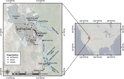
The GSL is a unique body of water, with an average depth of approximately 4.2 meters. It is characterized as a hyper-saline lake, with salinity ranging from 11 to 15% in the southern half (US Geologic Survey [USGS] Utah Water Science Center 2013). Farmington Bay is approximately 1 m deep, with 1–8% salinity. Because these lakes are so shallow, surface area varies considerably with lake level. Following several exceptionally wet years in the early 1980s, the GSL and Farmington Bay had approximate surface areas of 2500 and 450 square kilometers, respectively. However, current surface areas of the GSL and Farmington Bay are approximately 1600 and 75 square kilometers, respectively. The GSL is the terminal point for several major rivers (Jordan, Weber, and Ogden rivers), and contains significant land and water-access areas for recreation and bird habitat. Farmington Bay supports a diverse ecosystem for millions of migratory birds that feed on the abundant insects and brine shrimp (Cox and Kadlec 1995) and features many popular recreation and camping spots. The GSL plays an important role in both the brine shrimp industry and recreation, with one of the few marinas and boat launches on the lake. Heavy use of the GSL through bird-watching, hunting, and other recreation draws hundreds of thousands of visitors each year, providing additional motivation for improving lake health and aesthetics. Additionally, the GSL provides a significant net economic value (between $10.3 million and $58.9 million annually) to publicly owned treatment works by serving as a receiving waterbody for wastewater discharge (Bioeconomics, Inc. 2012). The total contribution of all services and uses of the GSL (industrial, aquaculture, and recreational) to the Utah gross domestic product is estimated at $1.3 billion annually.

Utah Lake is also very shallow, with an average depth of approximately 2.74 m and a current approximate surface area of 340 square kilometers. In the mid-1980s, it was closer to 400 square kilometers. It has higher salinity than most freshwater lakes (around 0.1%), which fluctuates depending on inflows and evaporation (UDEQ 2006). Utah Lake has a number of campgrounds, public access points, and marinas supporting recreational activities. Like Farmington Bay, it also supports a large migratory bird population, and is heavily monitored because it is a habitat for the endangered June sucker (Chasmistes liorus) species.

Historically, diatoms have dominated Utah Lake, though many species of chlorophyta (green algae) and cyanobacteria (blue-green algae) have also been frequently observed (Rushforth and Squires 1985). Recent (since 2014) blooms in the mid to late summer in Utah Lake have largely been dominated by Microcystis, Aphanizomenon, and Dolichospermum (UDEQ 2018). In Farmington Bay, large blooms of cyanobacteria (especially Nodularia) have been observed, whereas the most prevalent algae in the GSL are diatoms and green algae (Wurtsbaugh 2008, Wurtsbaugh et al. 2012).

Previous studies of algal blooms in the Great Salt Lake system

As is the case with many large lakes, monitoring water quality at high spatial and temporal resolutions is not feasible in the GSL system. Traditional sampling techniques are costly and cannot reasonably cover the entire spatial extent of these large lakes. There also are limitations to data sharing (e.g., lags between when data are collected and when they are formatted and published) and differences in sampling methods among the various monitoring organizations. These organizations include the Utah Department of Environmental Quality Division of Water Quality (UDWQ), the US Geological Survey (USGS), and the Jordan River/Farmington Bay Water Quality Council (JRFBWQC). Historically, these organizations have used chlorophyll a (Chl-a) concentrations to estimate algae biomass at set locations throughout the lake system (Figure 1).

In the past, remote sensing of HABs in the GSL system was limited to single events. One study used Earth Resources Technology Satellite (ERTS-1) and aerial imagery from a single date to describe the distribution of an algal bloom in Utah Lake (Strong 1974); however, there were no estimates of algal biomass. More recently, a study of the 2016 Utah Lake bloom used Sentinel-2A and Landsat 8 to estimate the Floating Algae Index and the Normalized Difference Chlorophyll Index (Page et al. 2018). The Page et al. study did not attempt to calibrate site-specific models or account for unique physical or optical characteristics of Utah Lake, but relied on models from the literature.

Previous studies of algal bloom drivers in the GSL system have largely focused on field-measured or laboratory-controlled Chl-a and in-lake characteristics and constituents (e.g., water temperature, nutrient and salinity concentrations) (Wurtsbaugh 2008, Goel and Myers 2009, Larson and Belovsky 2013, Marden et al. 2015). Study of any external factors (e.g., hydrology or meteorology) has been limited to Utah Lake and a single bloom event (Page et al. 2018). Our study extends previous work by using nontraditional methods (i.e., remote sensing) to estimate Chl-a and by exploring trends and effects of external factors using a long record of Chl-a conditions.

Methods

A review of analytical/semi-analytical (based on bio-optical models) and empirical (based on observed relationships between limnological and remotely sensed data) approaches to remote sensing of water quality (Matthews 2011) shows that both approaches have been demonstrated for a wide range of inland lake and reservoir systems. While the physical processes modeled by analytical approaches are important for certain contexts (i.e., understanding scattering/absorption characteristics of water constituents (International Ocean-Colour Coordinating Group [IOCCG] 2006), this study uses an empirical approach, due to its relative simplicity and ability to exploit available historical data. Information about other constituents affecting inherent optical properties in the study area is limited, hindering the development of analytical models. For example, an analytical model of Utah Lake would require historical information about calcite precipitation (which affects water color); however, coincident historical data are not readily available. Empirical modeling approaches inherently account for conditions that affect spectral features without requiring detailed information on the physical parameters. We used an empirical modeling approach to estimate Chl-a, and statistical analyses to evaluate trends and relationships of Chl-a to local climate conditions throughout the GSL system.

Data

Field measurements

We obtained historical field-measured surface Chl-a concentrations from the UDWQ using the Ambient Water Quality Monitoring System (AWQMS) database (from 1995 to 2012), from the USGS using the National Water Information System (NWIS) (from 1995 to 2015), and JRFBWQC (from 1997 to 2015) (Table 1). Data were limited to measurements during the main growing season (May–Sep). The number of observations for Utah Lake, GSL, and Farmington Bay during these time periods were 325, 1148, and 95, respectively. The map of sampling locations (Fig. 1) and limited number of historical samples for these 3 organizations highlight the temporal and spatial limitation of the existing records.

Table 1. Summary data used for model development, application, and analysis.

Data source	Data type	Period of record	Resolution or units
UDWQ	Surface chlorophyll a	1992–2009	µg/L
USGS	Surface chlorophyll a	1995–2015	µg/L
Jordan River/Farmington Bay Water Quality Council	Surface chlorophyll a	2013	µg/L
Landsat-5 TM	Surface reflectance	1984–2007	30 m pixels, 16-d satellite overpass
Landsat-7 ETM+	Surface reflectance	1999–2016	30 m pixels, 16-d satellite overpass
National Climate Data Center	Daily precipitation, daily average wind speed, daily total wind movement, daily maximum air temperature	1984–2016	mm/d, m/s, km/d, degrees Celsius
Natural Resources Conservation Service	Snow water equivalent (SWE)	1984–2016	inches/d

Chl-a concentrations are the most common index of algal biomass used by local monitoring organizations. For the GSL and Farmington Bay, the data used in calibration were corrected for the accessory pigment pheophytin; however, the available record for Utah Lake mostly contained measurements that were not corrected for pheophytin. In the few available records containing both uncorrected and corrected Chl-a, measurements, the corrected Chl-a concentrations were generally around 30% lower than the uncorrected concentrations. To maintain consistency, we used only the uncorrected Chl-a concentrations for calibrating the Utah Lake models. Measurements for all of the lakes were taken near the surface, at depths <1 m (generally <0.25 m). For dates where samples at multiple depths were collected, we used the measurement nearest the surface.

Satellite imagery and Google Earth Engine

The satellite imagery used for this study was acquired by the NASA Landsat-5 Thematic Mapper (TM), launched in 1984, and Landsat-7 Enhanced Thematic Mapper Plus (ETM+), launched in 1999 (Table 1). These instruments collect 30 m resolution imagery covering the major global land surfaces (including all of North America) at a revisit rate of 16 d. This means the satellite repeats coverage for each scene within the Landsat Worldwide Reference System (WRS), a grid reference system of 233 paths and 248 rows, once every 16 d. The GSL system is contained within Path 38, Row 32 and Path 38, Row 31 of the WRS. There are slight variations in Bands 4 and 7 between the 2 missions that are assumed to be negligible. This allows for development of models that produce estimates with either Landsat-5 or Landsat-7 images. We chose not to include Landsat 8 in the analysis due to the lack of available calibration data during its operational period.

We obtained imagery data through Google Earth Engine (Gorelick et al. 2017) to reduce the burden of data management, storage, and processing. Earth Engine has been used in a wide variety of land cover/waterbody classification (Alonso et al. 2016) and flood and surface water mapping (Pekel et al. 2016, Tellman et al. 2016) studies, and less extensively for accessing and processing data for algal bloom monitoring (Ho et al. 2017). We created functions using the Earth Engine Python Application Programming Interface to query the online server and return the surface reflectance values for the GSL system as a dataframe that could be used within R statistical software (R Core Team 2018) for model development and application. The Landsat surface reflectance products available through Earth Engine are generated by the USGS (USGS 2018) using the Landsat Ecosystem Disturbance Adaptive Processing System (LEDAPS) (Masek et al. 2006), which converts the top of atmosphere reflectance to surface reflectance. The long, continuous record and ready availability of these data products allow for a convenient exploration of the historical record. However, we note that the use of LEDAPS introduces potential errors into the modeling process. The LEDAPS method removes atmospheric contributions to the at-sensor radiance when calculating the remote sensing surface reflectance (R_rs); however, the LEDAPS approach can sometimes overcorrect for atmospheric interference, resulting in negative reflectance values over water in the short-wave infrared range (where water surface reflectance is typically very low). This is generally most problematic in deep, clear waterbodies that appear very dark and have low signal-to-noise ratio; however, the lakes in the GSL system are generally turbid and shallow. We removed negative reflectance values and excluded them from model calibration and application. The Landsat surface reflectance product includes a cloud mask and cloud mask confidence band, which allows filtering of pixels that are obstructed by cloud cover or haze. We used the cloud mask information to ensure that only cloud-free pixels were included in the model development and application. We also masked pixels from Landsat 7 data that were affected by scan line corrector error (present in images after May 31, 2003), allowing the rest of the image with valid data to be used in the calibration and application workflow.

For each field sample, we obtained surface reflectance values (from the pixel corresponding with the field sampling location) for every image within ±10 d of the sample date. If pixels from multiple images were returned for a single field sample, we used the reflectance values from the image nearest the sampling date (unless there was cloud cover).

Climate data

We obtained historical daily meteorological records matching the record of remotely sensed imagery (1984–2016) from the National Oceanic and Atmospheric Administration (NOAA) National Climate Data Center archives for stations near the Great Salt Lake and Farmington Bay (USW00024127, located at 40°46′21″N, −111°57′19.01″W) and Utah Lake (USC00428973, located at 40°22′0.01″N, −111°54′0″W). These stations provide the most complete record for precipitation (mm/d), wind speed (m/s) or total daily wind movement (km), and maximum/minimum daily temperature (degrees Celsius) near the study area. Additionally, estimates of snow water equivalent (SWE) in inches were obtained from Natural Resources Conservation Service Snow Telemetry (SNOTEL) sites: Site 820, located at 40°26′N, −111°37′W, and Site 684, located at 40°46′N, −111°38′W. Site 820 is assumed to be representative of snowpack for watersheds contributing to Utah Lake, while site 684 is representative of snowpack for the GSL and Farmington Bay watersheds.

Model parameterization

Our model development approach is data driven (using statistical techniques to determine model parameterization) while being rooted in observations of physical characteristics and processes (creating unique models for the distinct lakes and seasons and using appropriate near-coincident data). Parameterization of empirical Chl-a models (the selection of bands, band ratios, and band combinations) can be difficult because of the range of models used in the literature for different types of waters, physical characteristics, presence of other constituents, and levels of turbidity (Gurlin et al. 2011, Matthews 2011, Lesht et al. 2013, Ali et al. 2014, Hansen and Williams 2018). Optimal band selection for the unique water chemistry and characteristics of the GSL system is further complicated by seasonal algae succession. Succession results in reflective properties that are specific to the dominant populations of algae at different times of the growing season (Casterlin and Reynolds 1977, Stadelmann et al. 2001, Hansen et al. 2015). A pattern of algae succession is documented for Utah Lake, with high species diversity in early summer months and a reduction in species diversity and domination of blue-green algae in later months (Whiting et al. 1978, Rushforth et al. 1981, Rushforth and Squires 1985).

To reflect the unique physical characteristics of the system and exploit variations in algae populations, we considered all TM/ETM + bands, band ratios, and the Normalized Difference Vegetation Index as potential predictor variables in a series of lake- and season-specific stepwise regressions. We did not limit to bands used in the literature, which have been shown to perform poorly for these lakes (Hansen and Williams 2018). We used a generalized linear model (GLM) structure with log-link functions to account for the nonnormal distribution of Chl-a data (Nelder and Wedderburn 1972) and a mixed stepwise regression based on minimizing the Akaike information criterion (AIC) to provide an initial suite of predictor variables. The AIC is particularly useful for evaluating models with different numbers of parameters, as it penalizes models with more parameters (similar to an adjusted R² value). We further refined the initial parameters from the stepwise regression to include only highly significant parameters (p < 0.05). This approach resulted in 2 models for each lake: 1 for spring (May–Jun) and 1 for summer (Jul–Sep), resulting in 6 final models.

For calibration, we used near-coincident sample data because historical water quality data were collected without respect to the satellite overpass schedule, resulting in relatively few exact matches. While water clarity studies have used a wide range of time windows to match sampled and remotely sensed data (ranging from ±3 h [Bailey and Werdell 2006], to 1 d [Lesht et al. 2013], 7 d [Kloiber et al. 2002, McCullough et al. 2013], and ±10 d [Olmanson et al. 2008]), a shorter time window may be more appropriate for estimating Chl-a due to the episodic nature of algal bloom events. Previous Chl-a studies in nearby Utah lakes noted an improvement in model performance with shorter time windows between 0 and 1 d (Hansen et al. 2015). To determine an appropriate time window for the final models in this system, we used observations of temporal variability in the lake system (Hansen et al. 2017), which indicated high variability and low autocorrelation for Utah Lake after 2 d, and less variability and higher autocorrelation in Farmington Bay and GSL. This suggests time windows of less than 2 d would be appropriate for Utah Lake and more relaxed time windows could be considered for the others. We further justified the time window by comparing model performance (R² between modeled and observed values) for each time window from ±0 to 10 d (Fig. S1). R² generally decreased as the time window was relaxed, with the exception of the GSL-Summer model, which had a better model fit with a time window of ±2 d compared to 0 or 1 d (due to a significant increase in the number of observations and broader range of Chl-a). No models were developed for Farmington Bay using time windows less than 2 d due to insufficient data. The final time windows, based on the observational data and the exploration of different time windows, were defined as ±1 d for Utah Lake, ±2 d for GSL, and ±4 d for Farmington Bay.

Final model coefficients and parameters are provided (Table 2). Model goodness of fit was measured via percent bias (PBIAS), which is calculated as follows: (1) $$\mathit{PBIAS}=100\mathrm{*}\frac{\sum ({\mathit{Mod}}_i-{\mathit{Obs}}_i)}{{\sum \mathit{Obs}}_i}$$(1) where Mod_i and Obs_i are corresponding values for each ith observation of Chl-a from the modeled and calibration datasets. PBIAS for the final models ranges from −15.9 to 17% (Table 2). Positive values indicate overestimation bias, whereas negative values indicate model underestimation bias. Other measures of goodness of fit include R² between the modeled and observed Chl-a (ranging from 0.79 to 0.99; Table 2 and Fig. 2) and mean absolute error (MAE) between modeled and observed values. The magnitude of the MAE is generally low (1–13.4 µg/L). This corresponds to 9–48% of the mean observed Chl-a or 2–8% of the maximum observed Chl-a. The exception to this is the Spring Farmington Bay model, which has a MAE of 38.5 µg/L, where there were relatively few data available for calibration and the magnitudes and range of concentrations were much greater than for other lakes and seasons (normalized to mean and maximum observed Chl-a, the MAE is 19 and 8%, respectively). While the normalized MAE with respect to mean is relatively high, model residuals have no apparent patterns or trends and approximate a normal distribution, indicating that the models do not consistently produce larger errors for any particular range of Chl-a concentrations.

Figure 2. Modeled versus observed Chl-a, with R² between modeled and observed values. Differences between the solid regression line and the dashed 1:1 line show the under-/overestimation.

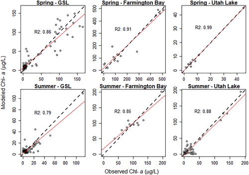
Table 2. Summary of model characteristics and performance. Performance is measured via R², mean absolute error (MAE), and percent bias (PBIAS) between modeled and observed Chl-a concentrations.

Lake	Season	Number of near coincident matches	Time window (±days)	Range of Chl-a in calibration data (µg/L)	Modeled vs. observed R^2	MAE (µg/L)	PBIAS	Model
Utah Lake	May–Jun	10	1	1.2–45	0.99	0.9	−0.3%	Chl-a = exp(−14.23 + 9.33*Green/Blue + 0.003*Blue − 0.004*SWIR1)
	Jul–Sep	46	1	0.2–185.5	0.88	10.6	−15.9%	Chl-a = exp(7.33 - 0.004*Blue − 0.05*Green/SWIR2 + 0.01*Red/SWIR1)
Great Salt Lake	May–Jun	90	2	0.3–164.2	0.86	10.9	17.0%	Chl-a = exp(3.51 + 0.09*Green/Blue − 0.01*Blue + 0.009*Red)
	Jul–Sep	69	2	0.045–112	0.79	5.2	−3.0%	Chl-a = exp(−0.36 + 6.12*Red/Blue − 0.006*Red)
Farmington Bay	May–Jun	14	4	4–505.9	0.87	38.5	1.4%	Chl-a = exp(6.53 - 1.02*Red/NIR − 0.009*SWIR2 + 0.004*SWIR1)
	Jul–Sep	11	4	37.38–196	0.86	13.4	0.2%	Chl-a = exp(6.11 − 0.002*Green)

Model application

We applied the calibrated models to water-masked, cloud-free surface reflectance data from 1984 to 2016. We then computed a modified normalized difference water index (MNDWI), which was developed specifically for distinguishing waterbodies in Landsat imagery (Xu 2006), and applied the results to each scene to mask nonwater pixels. This is to account for variation in lake surface area over time and ensure only water pixels were included in lake-wide summaries. The MNDWI equation uses the mid-infrared band (band 5 or B5) and the green band (band 3 or B3) in Landsat 5 and 7 imagery, as shown in Equation 2:(2) $$\mathit{MNDWI}=\mathrm{ }\frac{B3-B5}{B3+B5}$$(2) (2) $$\mathit{MNDWI}=\mathrm{ }\frac{B3-B5}{B3+B5}$$(2)

Positive MNDWI values were considered water, while negative MNDWI were classified as land (Xu 2006). We assumed that any estimated Chl-a concentrations above 500 µg/L were noise and masked them from the final results.

Statistical analysis

Trends

We calculated long-term trends of the change in Chl-a (µg/L per year) over the resulting historical record using the nonparametric Theil–Sen estimator, which is robust for nonnormally distributed data and outliers (Esterby 1996). The Theil–Sen slope estimator is calculated as the median of the slopes of the lines crossing all possible pairs of distinct points. Its use in water quality time-series analysis has been demonstrated in literature (Esterby 1996), particularly when the time series is irregular or when time series exhibit seasonality (Hirsch et al. 1982). We used the Median-Based Linear Models, or mblm package, in R (Komsta 2013) to calculate the Theil–Sen estimator for each of the lakes over the 32-yr constructed record. We calculated annual trends for a number of characteristics describing algal bloom dynamics. These include mean, extreme (99th percentile), variability (standard deviation), and spatial extent (calculated as a percentage of pixels above 50 µg/L, which corresponds to highly eutrophic and hypereutrophic conditions, according to the Carlson TSI metric [Carlson 1977]). We also calculated long-term trends by month to examine potential seasonality (Hirsch et al. 1982). Finally, we calculated trends in the timing of annual maximum Chl-a values (day of year when the estimated maximum Chl-a level occurred) using the Theil–Sen estimator.

Influence of short-term weather and seasonal climate conditions

Short-term meteorological conditions (including wind, precipitation, and high air temperatures) may affect surface Chl-a concentrations by contributing to mixing or providing a favorable environment for algae growth and buoyancy with calm conditions and higher water temperatures (Fig. S2). These short-term events could have immediate effects at timescales that are relevant to sampling or short-term monitoring. We evaluated relationships between these parameters and Chl-a by determining quartiles for each meteorological variable and sorting estimates of Chl-a into groups or subsets based on the conditions of the previous day. We then evaluated differences between the means of these subsets using the Kruskal–Wallis test, a nonparametric test to evaluate whether differences between the subsets is significant (p < 0.05). We also used the nonparametric Kendall’s tau method to measure the strength of the relationship between the meteorological variable and Chl-a concentrations across the entire range of possible meteorological conditions, with a null hypothesis that there is no association between Chl-a and the variables.

We also evaluated whether the seasonal climate conditions that were identified as likely triggers by Page et al. (2018) for the 2016 bloom are supported by evidence in the remotely sensed record. The study of the 2016 bloom suggested that the major drivers were high winter and spring (Dec–Mar) precipitation, high spring (Mar) runoff, and low precipitation and warmer temperatures in early summer months (May–Jun). Instead of modeled climate and hydrology data, we used weather observations from NOAA stations during the same seasons defined by Page et al. (2018) and we used SWE observations from SNOTEL sites during March a proxy for runoff (which is largely driven by snowpack, and March is typically when the peak SWE occurs in these watersheds [Fig. S3]). Trends in the seasonal climate parameters (temperature, precipitation, and SWE) were evaluated using the Theil–Sen estimator.

To evaluate whether the conditions identified by Page et al. (2018) were consistent with algal bloom conditions in the past, we first calculated precipitation totals, average temperatures, and average SWE for the seasons defined above. Page et al. (2018) did not indicate how the 2015–2016 climate conditions compared to typical conditions; rather, they compared values to those in other months in the year leading up to the bloom. This is problematic, as it mostly describes the general seasonal climate patterns of the study area (higher precipitation in winter and spring, high runoff in the spring, and low precipitation and higher temperatures in early summer). Instead, we used a relative comparison to the averages of the historical period (1984–2016), and subset the 32-yr record of annual Chl-a measures according to above historical average and below historical average seasonal conditions. The conditions that were suggested as contributing to the 2016 bloom were high precipitation in December–March, high March SWE, and low precipitation and high temperatures in May–June. Similar to the comparison of short-term conditions, we evaluated the statistical significance of differences in these subsets using the Kruskal–Wallis test, and also used Kendall’s tau to evaluate correlations over the entire range of seasonal climate conditions.

Additional information about the tools and software packages developed to accomplish the model calibration, application, and postapplication analysis workflow (Fig. S4) is provided in the supplementary information.

Results

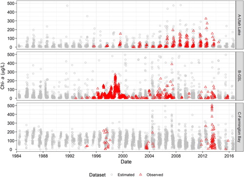
The empirical models we developed produce a remotely sensed record that supplements and enhance the field sampling record by greatly increasing the extent and the number of Chl-a estimates (Fig. 3). The remotely sensed estimates extend the field sampling records more than a decade earlier than the field record and provide more complete seasonal records than the field sampling record. There were approximately 7 times more remotely sensed estimates than field samples for Utah Lake and GSL, and 34 times more for Farmington Bay (which had the most severely limited field sampling record). The increase in the number of data available for analysis reduces uncertainty in the results of statistical analyses of trends and relationships. The models also increase the spatial information available for the lake system by providing estimates of such as lake-wide averages, lake-wide extremes, and spatial extent of blooms.

Figure 3. Historical record of Chl-a concentrations between 1984 and 2017 for the sampling locations in the Great Salt Lake System: (A) Utah Lake, (B) Great Salt Lake, and (C) Farmington Bay. The observed data (triangles) are from field samples and the estimated (circles) are from remotely sensed imagery.

Trends in the constructed historical record

Over the 32-yr remotely sensed record, the lake system shows significant increasing trends of extreme Chl-a values (1.8–4.9 µg/L per year) and Chl-a variability (0.2–1.2 µg/L per year) (Table 3). Farmington Bay and Utah Lake have slight decreasing trends in the spatial extent of blooms, and Utah Lake has a slight decreasing trend in the average Chl-a. The trends from the remotely sensed record contrast those observed in the more limited field sampling record. Notably, trends based on field sampling records for Utah Lake indicate increases in average Chl-a (3.1 µg/L per year) instead of a slight decrease, and relatively large increases in extremes (13.3 µg/L per year), and variability (3.3 µg/L per year). Field sampling-based trends for the GSL and Farmington Bay also differ from remotely sensed-based trends, indicating no significant trends for average, extremes, or variability.

Table 3. Summary of statistically significant (α = 0.05) long-term trends (change per year), calculated using the Theil–Sen estimator from 1984 to 2016.

Lake	Average Chl-a (µg/L/yr)	Extreme Chl-a (µg/L/yr)	Standard deviation of Chl-a (µg/L/yr)	Bloom extent (%/yr)	Timing of peak average Chl-a (d/yr)	Timing of peak extreme Chl-a (d/yr)
Utah Lake	−0.25	1.8	0.2	−0.2	−1.2	−0.5
Great Salt Lake	—	2.8	0.55	—	−1.5	−2.5
Farmington Bay	—	4.9	1.2	−0.4	−2.5	−1.2

Long-term trends of the timing of blooms (i.e., day of year when average and extreme Chl-a concentrations peaked) exhibit a statistically significant (p < 0.05) shift to earlier in the growing season. These trends range from 1.2 to 2.5 d earlier per year for peaks in average concentrations and 0.5–2.5 d earlier per year for peaks in extreme values (Table 3). Assuming a perfectly linear pattern, this means peaks in average concentrations are now occurring between 5 and 11 weeks earlier and peaks in extremes are occurring 2–11 weeks earlier compared to the early 1980s.

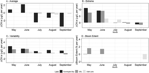
Seasonally, the long-term trends in the lake system are more nuanced (Fig. 4). The data show trends of increasing averages and extremes in the system in May and June, while July through September generally exhibit decreasing trends (or in some cases, smaller positive trends compared to those observed in the earlier months). The earlier months also exhibit trends of increasing variability and in the case of the GSL, increasing spatial extent of blooms. The pattern of increasing averages and extremes in earlier months, along with shifts in the timing of peak average and extreme concentrations, indicates that poor conditions in the lake system are occurring earlier in the season than they did in the past.

Figure 4. Magnitudes of trends for lake-wide (A) average (mean) Chl-a, (B) extreme (99th percentile) Chl-a, (C) variability (standard deviation) of Chl-a, and (D) bloom extent (as a percent of lake >50 µg/L). Only statistically significant trends are shown. Note increasing trends in early summer months for average and extreme concentrations, increasing trends in variability for the whole growing season, and increasing trends for bloom extent in the early summer months in the GSL.

The long-term shifts in seasonality of peak Chl-a timing and early summer averages and extremes are coincident with general long-term trends in the local climate. During the same period (1985–2016), there is an increase in temperature during most months for both sites, and a decrease in precipitation and SWE (particularly for the Utah Lake weather monitoring sites) (Fig. S4). While a combination of influences may contribute to a bloom in any given year (including those influences and scales explored in this study as well as other influences like natural and anthropogenic nutrient loading), it is important to recognize that these climate parameters are also exhibiting long-term changes and may be contributing to the shift in seasonal patterns.

Short-term influence of meteorological conditions

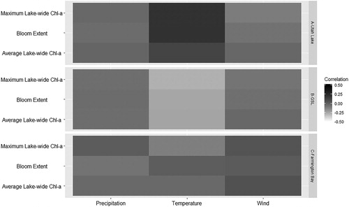
Relationships between surface Chl-a and preceding weather conditions were highly variable between the lakes in the GSL system and among sites within the lakes. While precipitation and wind are largely uncorrelated to each of the lake-wide measures of blooms for the entire system (Fig. 5), air temperature showed weak but significant (p < 0.05) correlations for Utah Lake and GSL (0.2 and −0.25, respectively). This may reflect some level of seasonality (where algae populations change throughout the season) and distinct algae populations that thrive under different temperature conditions.

Figure 5. Correlation between lake-wide bloom measures and meteorological parameters, as measured by Kendall’s tau for (A) Utah Lake, (B) GSL, and (C) Farmington Bay. The only significant correlations are between bloom measures and temperature (positive for Utah Lake, and negative for GSL).

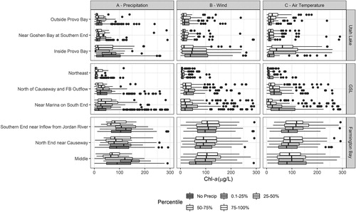
To further highlight the variability in short-term effects on Chl-a, we show differences in Chl-a at several sites throughout the system (Fig. 6). These sites are chosen for proximity to human activity or inflows or to show conditions throughout each of the lakes. Precipitation appears to have the biggest effect at sites near inflows (inside Provo Bay in Utah Lake and at the southern end and middle of Farmington Bay). At these sites, Chl-a is lower following medium to high precipitation compared to no or low precipitation (Fig. 6a). In contrast, sites in GSL showed little sensitivity to precipitation. Wind had the largest effect on the site inside Provo Bay, with high wind resulting in lower Chl-a, but no other sites showed much sensitivity (Fig. 6b). Temperature effects varied widely across the lakes and sites; following high temperatures, there were small increases in the Farmington Bay sites, large increases in the mean and variability in the Provo Bay site, but a pattern of decreasing mean and variability in GSL sites (Fig. 6c). The only meteorological condition that exhibited statistically significant differences in Chl-a was temperature; the sites in and near Provo Bay generally had higher Chl-a at higher quantiles and sites in GSL generally had lower Chl-a at higher quantiles showing.

Figure 6. Differences in distributions of Chl-a concentrations for selected sites in Utah Lake, GSL, and Farmington Bay. Chl-a is grouped according to the meteorological conditions of the previous day: (A) precipitation, (B) wind, and (C) maximum air temperature). Note the difference in sensitivity to different meteorological conditions between the lakes and between different locations in the same lake.

Influence of seasonal climate conditions

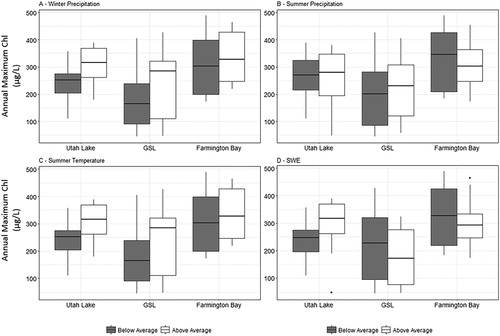
The evaluation of annual extreme Chl-a concentrations of Utah Lake largely supports the findings of Page et al. (2018), who suggested that a combination of high winter precipitation, low summer precipitation, high summer temperatures, and high runoff were responsible for the 2016 Utah Lake bloom. The estimated annual extreme Chl-a concentrations in Utah Lake were higher during years with these seasonal conditions (Fig. 7), with the exception of low summer precipitation, where there was very little difference between Chl-a during low or high summer precipitation (Fig. 7b). Extreme Chl-a levels in GSL and Farmington Bay were also generally higher during years with high winter precipitation and summer temperatures, but both lakes showed a decrease in extremes during years when there was high SWE (Fig. 7d). This highlights another difference between the lakes in this system and points to potential differences in the distinct watershed and loading processes during years with high snowpack/runoff. The only seasonal climate parameters that showed statistically significant differences in mean Chl-a were SWE and winter precipitation for Utah Lake, which had weak but significant positive correlations (r = 0.31 and 0.34, respectively). This further supports the idea that winter precipitation and SWE in the early spring are contributors to algal bloom conditions in Utah Lake. No other parameters and bloom measures in other lakes had statistically significant differences in means or correlations.

Figure 7. Distributions of annual extreme Chl-a concentrations, grouped by the condition of the seasonal climate parameters: (A) winter precipitation, (B) summer precipitation, (C) summer temperature, and (D) SWE. For Utah Lake, differences in extreme values generally follow the conditions suggested by Page et al. (2018); high Chl-a coincides with high winter precipitation, summer temperature, and SWE.

Discussion

Analysis of long-term trends indicates there has been a shift over the past several decades in the timing of algal blooms, with positive trends in the earlier months for several algal bloom dynamics and trends for peak conditions shifting earlier in the growing season. There are also positive trends in the annual extremes and variability over the last 3 decades. These increasing trends are occurring in a lake system where local summer temperature also increased. The shifting in timing and positive trends in extremes occurred coincidentally with increases in temperature and decreases in precipitation, which could be especially problematic in the face of future changing climate conditions. For example, differences in precipitation patterns and warming temperatures could create favorable conditions for extending the season of algal blooms. Future monitoring and management efforts may need to adjust for the seasonal shifts to plan for the emergence of blooms and poor conditions.

Localized sensitivity to short-term meteorological events provides important context for evaluating field sampling results (whether the sampled concentrations might be temporarily higher or lower because of a short-term meteorological condition). This could also aid in predicting likely movement of algae and areas that are susceptible to increases following storms, high winds, or periods of above-average temperatures. Knowledge of where blooms are likely to concentrate, spread, or move due to wind force/mixing could be helpful in tracking blooms, targeting sampling efforts, and making decisions dealing with closure or warnings for public recreational areas. Additionally, patterns of algal bloom movement may help inform hydrodynamic modeling efforts by providing insight into the sensitivity of algal blooms to certain factors like wind speed and surface mixing.

The long-term remotely sensed record supports the suggestion that high winter/spring precipitation, high temperatures, and high runoff contribute to algal blooms in Utah Lake, as these conditions coincided with years with more extreme Chl-a concentrations. However, algal bloom formation in Farmington Bay and GSL appears to be less affected by seasonal precipitation (and subsequent surface runoff) than in Utah Lake. These differences underscore the complexity of the lake system, the watershed processes that contribute the lake, and the diverse factors that influence algal bloom dynamics.

The trends for the estimated record (limited to estimates at historical monitoring locations) differed significantly from the record of field observations. The large difference in trends between the estimated and field sampling records can be attributed to varying numbers of samples (resulting in different distributions of Chl-a) over the length of the record. Likewise, trends in timing of annual maxima differ from those in the field sampling record. The remotely sensed record indicates an earlier shift in timing for all of the lakes, while the field sampling record indicates a trend of later peak conditions for Utah Lake. According to the record based only on field observations (which are limited to the sampling locations), the timing of the highest average Chl-a concentrations is occurring 2.7 d later each year, while the remotely sensed record (which is not limited to the sampling locations) indicates that the timing has shifted 1.2 d earlier each year. The differences in trends for the estimated and field-sampled records suggest that the irregular and inconsistent nature of the field sampling record and its limited spatial representation of the lakes could lead to incorrect conclusions about water quality behavior in the lake system.

Limitations

While the remotely sensed record we produced provides many benefits, it is important to note the limitations of this study. These include limitations of the remotely sensed data: suboptimal band configuration and surface reflectance products (as discussed previously), and the revisit rate of historical Landsat imagery. While the resolution of spectral bands and range of the Landsat sensors are not as well suited for water quality applications as some other sensors (Palmer et al. 2015), Landsat data have been widely used for small-scale Chl-a mapping applications (Giardino et al. 2001, Duan et al. 2007, Allan et al. 2011) and long-term and regional studies of lake Chl-a (Brezonik et al. 2005, Duan et al. 2009, Torbick et al. 2013, Allan et al. 2015, Hansen et al. 2015, Ho et al. 2017). This is largely due to the consistent revisit rate, long history, and complete spatial coverage of most large lakes at a relatively high resolution. Landsat-based estimates provide valuable information about water quality conditions throughout large bodies of water over relatively long periods of time compared to other satellites with more optimal band configurations. Landsat imagery continues to be used in modeling algal blooms in inland lakes because it provides extensive records for observing long-term effects (Ho and Michalak 2017) and it supplements limited historical records of other sensors (Ho et al. 2017). The long historical record is especially useful where historical field sampling records are as limited as those for the lakes in the GSL system. Additionally, the 16 d revisit rate could potentially miss entire bloom events, which reduces accuracy in estimates of the trends and timing of peak Chl-a concentrations. However, the remotely sensed record based on Landsat imagery still provides a much more complete view of long-term conditions than field records. Additionally, the failure of the Scan Line Correction in Landsat 7 images resulted in the loss of some data, which can also reduce accuracy of the trends.

Another limitation to the model development was the relatively limited historical data available for calibration (especially in Utah Lake and Farmington Bay). As a consequence of the limited calibration data and limitations of Landsat data, there were relatively large errors for the Farmington Bay spring model. These limitations may be resolved and the models may be improved as sustained records of better remote sensing products (such as newer satellites including Landsat 8 and Sentinel-2) become available and with increased monitoring that is coordinated with imagery acquisition. Several studies have demonstrated the use of these satellites for mapping of Chl-a (Manzo et al. 2015, Toming et al. 2016). These instruments can build on long-term studies using older instruments and provide data for recent history and ongoing monitoring applications. Future modeling efforts that build on these new data may still deal with limited available calibration data. We recommend coordination with monitoring agencies to optimize field sampling and encourage use of these data in remote sensing applications. Another limitation of this study is in the use seasonal approximations of algal succession and Chl-a as a measure of biomass. Increased information about seasonal algal speciation and potential shifts in species diversity (which is not currently available for the historical record) would improve the definition of seasonal models. Additionally, frequent collection of other measures, such as phycocyanin concentrations, would provide valuable information about whether the algal blooms are composed of cyanobacteria, and toxin levels would help identify blooms that are of particular interest for public health reasons.

Conclusions

This study identified several long-term changes in the water quality of the GSL system over the past several decades: shifts in peak Chl-a concentrations, increasing extremes, and increasing variability of Chl-a throughout the lakes. Lake managers must be able to anticipate and prepare for these changes by considering how future climate conditions could alter behavior and health of the lake system. Locations that are particularly sensitive to precipitation, high winds, and high temperatures may warrant additional consideration as the lakes are monitored in the future, and future sensor placement or timing/frequency of monitoring may need to be adjusted to account for this sensitivity.

The results and the patterns observed in the GSL system demonstrate the value of having an enhanced historical record, which provides more frequent and consistent observations and as greater spatial coverage than historical field sampling. This enhanced record allows for exploration of long-term trends, spatial patterns, and relationships to local climate conditions which are not feasible with limited field sampling-based records. The trends and connections to short-term climate events and longer term seasonal climate conditions should be used to guide local environmental and regulatory agencies as they focus resources and plan future monitoring efforts. In addition to the influences of the climate conditions explored in this study, other factors, such as nutrient loading from point and nonpoint sources in the surrounding area, should be studied to examine influence on the algal dynamics in the lake system. One of the main obstacles in doing so will be obtaining a long-term record of these contributions of nutrients.

As the improved remote sensing data and field data become available, the workflow and tools presented in this study for obtaining remotely sensed data, calibrating, and applying models can be adapted for future analysis and monitoring. This will enable water resource managers to identify and target problem areas, determine which conditions may be contributing to HAB problems, and evaluate whether conditions are worsening or improving. In turn, this encourages more effective monitoring and mitigation strategies, resulting in healthier and better managed lakes.

Acknowledgments

The authors thank Rob Baskin at the USGS, members of the JRFBWQC (now the Wasatch Front Water Quality Council), and Jake Van der Laan, Ben Holcomb, Marshall Baillie, and others at the UDWQ for providing feedback, assisting us in gathering historical data records, and collaborating on field sampling efforts.

Additional information

Funding

This article was developed under assistance agreement number 835866-01 awarded by the US Environmental Protection Agency to Dr. Michael Barber. It has not been formally reviewed by EPA. The views expressed in this document are solely those of the authors and do not necessarily reflect those of the agency. EPA does not endorse any products or commercial services mentioned in this publication.

References

- Acuña WC, Gonzalez CJ, Aqueveque VG. 2017. La Chimba, Antofagasta, Chile—oxygen depletion and hydrogen sulfide gas mitigation due to harmful algal blooms. Harmful algal blooms (HABs) and desalination: a guide to impacts, monitoring, and management. In: Anderson DM, Boerlage SFE, Dixon MB, editors. Paris (France): United Nations Educational, Scientific, and Cultural Organization (UNESCO). p. 391–8.
- Ali K, Witter D, Ortiz J. 2014. Application of empirical and semi-analytical algorithms to MERIS data for estimating chlorophyll a in case 2 waters of Lake Erie. Environ Earth Sci. 71(9):4209–20. doi:10.1007/s12665-013-2814-0.
- Allan MG, Hamilton DP, Hicks BJ, Brabyn L. 2011. Landsat remote sensing of chlorophyll a concentrations in central North Island lakes of New Zealand. Int J Remote Sens. 32(7):2037–55. doi:10.1080/01431161003645840.
- Allan MG, Hamilton DP, Hicks BJ, Brabyn L. 2015. Empirical and semi-analytical chlorophyll a algorithms for multi-temporal monitoring of New Zealand lakes using Landsat. Environ Monit Assess. 187(6):364.
- Alonso A, Muñoz-Carpena R, Kennedy RE, Murcia C. 2016. Wetland landscape spatio-temporal degradation dynamics using the new Google Earth Engine cloud-based platform: opportunities for non-specialists in remote sensing. Trans ASABE. 59:1331–42.
- Anderson DM, Glibert PM, Burkholder JM. 2002. Harmful algal blooms and eutrophication: nutrient sources, composition, and consequences. Estuaries. 25(4):704–26. doi:10.1007/BF02804901.
- Arnow T, Stephens DW. 1990. Hydrologic characteristics of the Great Salt Lake, Utah, 1847-1986. US Geological Survey Water-Supply Paper.
- Backer LC, McNeel SV, Barber T, Kirkpatrick B, Williams C, Irvin M, Zhou Y, Johnson TB, Nierenberg K, Aubel M, et al. 2010. Recreational exposure to microcystins during algal blooms in two California lakes. Toxicon. 55(5):909–21. doi:10.1016/j.toxicon.2009.07.006.
- Bailey SW, Werdell PJ. 2006. A multi-sensor approach for the on-orbit validation of ocean color satellite data products. Remote Sens Environ. 102(1-2):12–23. doi:10.1016/j.rse.2006.01.015.
- Bioeconomics, Inc. 2012. Economic significance of the Great Salt Lake to the State of Utah. Report for the Great Salt Lake Advisory Council. Missoula (MT): Bioeconomics, Inc.
- Brezonik P, Menken K, Bauer M. 2005. Landsat-based remote sensing of lake water quality characteristics, including chlorophyll and colored dissolved organic matter (CDOM). Lake Reserv Manage. 21(4):373–82. doi:10.1080/07438140509354442.
- Carlson RE. 1977. A trophic state index for lakes. Limnol Oceanogr. 22(2):361–9. doi:10.4319/lo.1977.22.2.0361.
- Casterlin ME, Reynolds WW. 1977. Seasonal algal succession and cultural eutrophication in a north temperate lake. Hydrobiologia. 54(2):99–108. doi:10.1007/BF00034983.
- Chen L, Delatolla R, D’Aoust PM, Wang R, Pick F, Poulain A, Rennie CD. 2017. Hypoxic conditions in stormwater retention ponds: potential for hydrogen sulfide emission. Environ Technol. 40:642–653.
- Cox RR, Kadlec JA. 1995. Dynamics of potential waterfowl foods in Great Salt Lake marshes during summer. Wetlands. 15(1):1–8. doi:10.1007/BF03160674.
- Duan H, Ma R, Xu X, Kong F, Zhang S, Kong W, Hao J, Shang L. 2009. Two-decade reconstruction of algal blooms in China’s Lake Taihu. Environ Sci Technol. 43(10):3522–8. doi:10.1021/es8031852.
- Duan H, Zhang Y, Zhang B, Song K, Wang Z. 2007. Assessment of chlorophyll-a concentration and trophic state for Lake Chagan using Landsat TM and field spectral data. Environ Monit Assess. 129(1-3):295–308. doi:10.1007/s10661-006-9362-y.
- Esterby SR. 1996. Review of methods for the detection and estimation of trends with emphasis on water quality applications. Hydrol Process. 10(2):127–49. doi:10.1002/(SICI)1099-1085(199602)10:2<127::AID-HYP354>3.0.CO;2-8.
- Falconer IR. 1999. An overview of problems caused by toxic blue–green algae (cyanobacteria) in drinking and recreational water. Environ Toxicol. 14(1):5–12. doi:10.1002/(SICI)1522-7278(199902)14:1<5::AID-TOX3>3.0.CO;2-0.
- Giardino C, Pepe M, Brivio PA, Ghezzi P, Zilioli E. 2001. Detecting chlorophyll, Secchi disk depth and surface temperature in a sub-alpine lake using Landsat imagery. Sci Total Environ. 268(1-3):19–29. doi:10.1016/S0048-9697(00)00692-6.
- Goel R, Myers L. 2009. Evaluation of cyanotoxins in the Farmington Bay, Great Salt Lake, Utah. Project Report. [accessed 2016 Oct 20]. http://www.cdsewer.org/GSLRes/2009_CYANOBACTERIA_PROJECT_REPORT.pdf
- Gorelick N, Hancher M, Dixon M, Ilyushchenko S, Thau D, Moore R. 2017. Google Earth Engine: planetary-scale geospatial analysis for everyone. Remote Sens Environ. 202:18–27. doi:10.1016/j.rse.2017.06.031.
- Gurlin D, Gitelson AA, Moses WJ. 2011. Remote estimation of Chl-a concentration in turbid productive waters—return to a simple two-band NIR-red model? Remote Sens Environ. 115(12):3479–90. doi:10.1016/j.rse.2011.08.011.
- Hansen CH, Burian SJ, Dennison PE, Williams GP. 2017. Spatiotemporal variability of lake water quality in the context of remote sensing models. Remote Sens. 9(5):409. doi:10.3390/rs9050409.
- Hansen CH, Williams GP. 2018. Evaluating remote sensing model specification methods for estimating water quality in optically diverse lakes throughout the growing season. Hydrology. 5(4):62. doi:10.3390/hydrology5040062.
- Hansen CH, Williams GP, Adjei Z, Barlow A, Nelson EJ, Miller AW. 2015. Reservoir water quality monitoring using remote sensing with seasonal models: case study of five central-Utah reservoirs. Lake Reserv Manage. 31(3):225–40. doi:10.1080/10402381.2015.1065937.
- Heisler J, Glibert PM, Burkholder JM, Anderson DM, Cochlan W, Dennison WC, Dortch Q, Gobler CJ, Heil CA, Humphries E, et al. 2008. Eutrophication and harmful algal blooms: a scientific consensus. Harmful Algae. 8(1):3–13. doi:10.1016/j.hal.2008.08.006.
- Hirsch RM, Slack JR, Smith RA. 1982. Techniques of trend analysis for monthly water quality data. Water Resour Res. 18(1):107–21. doi:10.1029/WR018i001p00107.
- Ho JC, Michalak AM. 2017. Phytoplankton blooms in Lake Erie impacted by both long-term and springtime phosphorus loading. J Great Lakes Res. 43(3):221–8. doi:10.1016/j.jglr.2017.04.001.
- Ho JC, Stumpf RP, Bridgeman TB, Michalak AM. 2017. Using Landsat to extend the historical record of lacustrine phytoplankton blooms: a Lake Erie case study. Remote Sens Environ. 191:273–85. doi:10.1016/j.rse.2016.12.013.
- Hunter P. 1998. Cyanobacterial toxins and human health. J Appl Microbiol. 84(1):35–40.
- [IOCCG] International Ocean-Colour Coordinating Group. 2006. Remote sensing of inherent optical properties: fundamentals, tests of algorithms, and applications. Dartmouth (Canada): Reports of the International Ocean-Colour Coordinating Group, No. 5.
- Kloiber SM, Brezonik PL, Olmanson LG, Bauer ME. 2002. A procedure for regional lake water clarity assessment using Landsat multispectral data. Remote Sens Environ. 82(1):38–47. doi:10.1016/S0034-4257(02)00022-6.
- Komsta L. 2013. mblm: median-based linear models. R package version 0.12 [accessed 2018 April 12]. https://CRAN.R-project.org/package=mblm.
- Larson CA, Belovsky GE. 2013. Salinity and nutrients influence species richness and evenness of phytoplankton communities in microcosm experiments from Great Salt Lake, Utah, USA. J Plankton Res. 35(5):1154–66. doi:10.1093/plankt/fbt053.
- Lesht BM, Barbiero RP, Warren GJ. 2013. A band-ratio algorithm for retrieving open-lake chlorophyll values from satellite observations of the Great Lakes. J Great Lakes Res. 39(1):138–52. doi:10.1016/j.jglr.2012.12.007.
- Manzo C, Bresciani M, Giardino C, Braga F, Bassani C. 2015. Sensitivity analysis of a bio-optical model for Italian lakes focused on Landsat-8, Sentinel-2 and Sentinel-3. Eur J Remote Sens. 48(1):17–32. doi:10.5721/EuJRS20154802.
- Marden B, Miller T, Richards D. 2015. Factors influencing cyanobacteria blooms in Farmington Bay, Great Salt Lake, Utah. A progress report of scientific findings from the 2013 growing season. Kaysville (UT): The Jordan River/Farmington Bay Water Quality Council.
- Masek JG, Vermote EF, Saleous NE, Wolfe R, Hall FG, Huemmrich KF, Gao F, Kutler J, Lim TK. 2006. A Landsat surface reflectance dataset for North America, 1990-2000. IEEE Geosci Remote Sensing Lett. 3(1):68–72. doi:10.1109/LGRS.2005.857030.
- Matthews MW. 2011. A current review of empirical procedures of remote sensing in inland and near-coastal transitional waters. Int J Remote Sens. 32(21):6855–99. doi:10.1080/01431161.2010.512947.
- McCullough IM, Loftin CS, Sader SA. 2013. Landsat imagery reveals declining clarity of Maine’s lakes during 1995-2010. Freshwater Sci. 32(3):741–52. doi:10.1899/12-070.1.
- Nelder JA, Wedderburn R. 1972. Generalized linear models. J Roy Statist Soc Ser A (Gen). 135(3):370–84. doi:10.2307/2344614.
- Olmanson LG, Bauer ME, Brezonik PL. 2008. A 20-year Landsat water clarity census of Minnesota’s 10,000 lakes. Remote Sens Environ. 112(11):4086–97. doi:10.1016/j.rse.2007.12.013.
- Page BP, Kumar A, Mishra DR. 2018. A novel cross-satellite based assessment of the spatio-temporal development of a cyanobacterial harmful algal bloom. Int J Appl Earth Obs Geoinf. 66:69–81. doi:10.1016/j.jag.2017.11.003.
- Palmer SC, Kutser T, Hunter PD. 2015. Remote sensing of inland waters: challenges, progress and future directions. Remote Sens Environ. 157:1–8. doi:10.1016/j.rse.2014.09.021.
- Paerl, HW. 1988. Nuisance phytoplankton blooms in coastal, estuarine, and inland waters. Limnology and Oceanography, 33(4, part 2), 823–843.
- Paerl, HW, Fulton, RS, Moisander, PH, Dyble, J. 2001. Harmful freshwater algal blooms, with an emphasis on cyanobacteria. The Scientific World Journal, 1, 76–113.
- Paerl, HW, Otten, TG. 2013. Harmful cyanobacterial blooms: causes, consequences, and controls. Microbial Ecology, 65(4), 995–1010.
- Pekel JF, Cottam A, Gorelick N, Belward AS. 2016. High-resolution mapping of global surface water and its long-term changes. Nature. 540(7633):418–22. doi:10.1038/nature20584.
- R Core Team. 2018. R: a language and environment for statistical computing. Vienna, (Austria): R Foundation for Statistical Computing. Available from https://www.R-project.org/.
- Rushforth SR, Squires LE. 1985. New records and comprehensive list of the algal taxa of Utah Lake, Utah, USA. Great Basin Nat. 45:237–54.
- Rushforth SR, St. Clair LL, Grimes JA, Whiting MC. 1981. Phytoplankton of Utah Lake. Great Basin Nat Mem. 5:85–100.
- Smith, VH. 2003. Eutrophication of freshwater and coastal marine ecosystems a global problem. Environmental Science and Pollution Research, 10(2), 126–139.
- Stadelmann TH, Brezonik PL, Kloiber S. 2001. Seasonal patterns of chlorophyll a and Secchi disk transparency in lakes of East-Central Minnesota: implications for design of ground-and satellite-based monitoring programs. Lake Reserv Manage. 17(4):299–314. doi:10.1080/07438140109354137.
- Strong AE. 1974. Remote sensing of algal blooms by aircraft and satellite in Lake Erie and Utah Lake. Remote Sens Environ. 3(2):99–107. doi:10.1016/0034-4257(74)90052-2.
- Tellman B, Sullivan J, Kettner A, Brakenridge G, Slayback D, Kuhn C, Doyle C. 2016. Developing a global database of historic flood events to support machine learning flood prediction in Google Earth Engine. AGU Fall Meeting Abstracts.
- Toming K, Kutser T, Laas A, Sepp M, Paavel B, Nõges T. 2016. First experiences in mapping lake water quality parameters with Sentinel-2 MSI imagery. Remote Sens. 8(8):640. doi:10.3390/rs8080640.
- Torbick N, Hession S, Hagen S, Wiangwang N, Becker B, Qi J. 2013. Mapping inland lake water quality across the Lower Peninsula of Michigan using Landsat TM imagery. Int J Remote Sens. 34(21):7607–24. doi:10.1080/01431161.2013.822602.
- [UDEQ] Utah Department of Environmental Quality 2006. Utah Lake report. Watershed Management Program.
- [UDEQ] Utah Department of Environmental Quality 2018. Harmful algal bloom events. [accessed 2019 Jan 10]. https://deq.utah.gov/legacy/divisions/water-quality/health-advisory/harmful-algal-blooms/bloom-events/index.htm.
- [USEPA] US Environmental Protection Agency. 2017. Recommendations for cyanobacteria and cyanotoxin monitoring in recreational waters. EPA/820/R-17/001. [accessed 2019 March 8]. https://www.epa.gov/sites/production/files/2017-07/documents/08_july_3_monitoring_document_508c_7.5.17.pdf
- [USGS] US Geologic Survey. 2018. Landsat 4-7 surface reflectance (LEDAPS) product guide. Version 1.0. Sioux Falls (SD): EROS.
- [USGS] US Geologic Survey: Utah Water Science Center. 2013. Great Salt Lake—salinity and water quality. [accessed 2017 Apr 5]. https://ut.water.usgs.gov/greatsaltlake/salinity/.
- Whiting MC, Brotherson JD, Rushforth SR. 1978. Environmental interaction in summer algal communities of Utah Lake. West North Am Nat. 38(1):31–41.
- Wurtsbaugh WA. 2008. Nutrient loading and eutrophication in the Great Salt Lake. Watershed Sciences Faculty Publications 299. [accessed 2018 June 19]. https://digitalcommons.usu.edu/wats_facpub/299
- Wurtsbaugh WA, Marcarelli A, Boyer G. 2012. Eutrophication and metal concentrations in three bays of the Great Salt Lake (USA). Final Report to the Utah Division of Water Quality, Salt Lake City, Utah.
- Xu, H. 2006. Modification of normalised difference water index (NDWI) to enhance open water features in remotely sensed imagery. International journal of remote sensing, 27(14), 3025–3033.