Long-term trends in inflowing chlorophyll a and nutrients and their relation to dissolved oxygen in a large western reservoir

Abstract

Naymik J, Larsen CA, Myers R, Hoovestol C, Gastelecutto N, Bates D. 2023. Long-term trends in inflowing chlorophyll a and nutrients and their relation to dissolved oxygen in a large western reservoir. Lake Reserv Manage. 39:53–71.

Anoxia in Brownlee Reservoir is one of the numerous water quality issues associated with eutrophic conditions in the Snake River as it flows through southern Idaho and parts of eastern Oregon. The states of Idaho and Oregon have developed total maximum daily loads (TMDLs) for multiple reaches of the Snake River and its tributaries upstream of Brownlee Reservoir intended to address poor water quality. Despite the emphasis on developing TMDLs throughout the Snake River and its tributaries, published long-term trend monitoring to evaluate the results of the TMDLs is lacking. Trends in Snake River concentrations and loads summarized using weighted regressions on time, discharge, and season show that combined efforts to improve water quality upstream of Brownlee Reservoir have realized decreasing trends in concentrations of chlorophyll a, total phosphorus, and suspended solids (80%, 46%, and 61% reductions, respectively) from 1995 to 2021. Brownlee Reservoir, a large mainstem reservoir with short residence time, has responded quickly to inflowing reductions of chlorophyll a and total phosphorus. Since 2005, dissolved oxygen (DO) has improved in the reservoir, with a 33% reduction in the volume of the reservoir having DO less than 1 mg/L. This supports the primary premise of upstream TMDLs and demonstrates that inflowing water quality improvements are effective at improving in-reservoir dissolved oxygen.

Keywords:

• Anoxia
• Brownlee Reservoir
• chlorophyll a
• Snake River
• total phosphorus

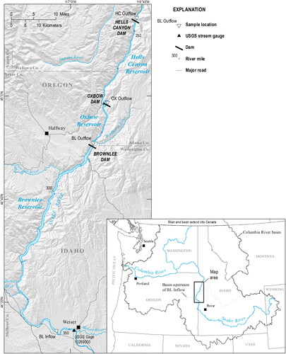
The Snake River flowing through southern Idaho is often referred to as a “working river,” with multiple water withdrawals, uses, impacts, and inputs from large-scale agriculture, hydroelectric reservoirs, municipalities, and other industry. Numerous water quality issues associated with eutrophic conditions occur, including heavy growth of aquatic macrophytes and suspended algae causing impacts to recreational uses (IDEQ and ODEQ 2004), low dissolved oxygen (DO) and high temperature impacting fisheries (Sullivan et al. 2003), harmful algal blooms occasionally causing livestock and pet deaths, and unhealthy levels of mercury in fish tissue (Clark et al. 2016, Baldwin et al. 2020, Baldwin et al. 2022). In the un-impounded reaches of the Snake River, many of these issues are exacerbated by low flow and slack water conditions partly due to large water withdrawals for irrigation (Worth 1995). State-led efforts (Idaho and Oregon) at improving conditions have resulted in the development of multiple total maximum daily loads (TMDLs) that apply to various reaches of the Snake River and its tributaries. One of these efforts is the Snake River–Hells Canyon TMDL (SR-HC TMDL; IDEQ and ODEQ 2004), which applies to the Snake River where it intersects the Oregon/Idaho border near Adrian, Oregon, and downstream nearly 220 miles (354 km) through the Hells Canyon wild and scenic reach of the river (IDEQ and ODEQ 2004). The scope of the SR-HC TMDL includes the Hells Canyon Complex, a series of 3 hydroelectric facilities spanning 100 miles (160 km) of the river, owned and operated by Idaho Power Company.

Brownlee Reservoir, the most upstream of the Hells Canyon Complex reservoirs, is large (1.76 km³), long (58 miles, 93 km), relatively narrow (less than 1.1 km wide), deep (maximum depth 91 m), and receives about 95% of its inflow from the Snake River. In-reservoir processes including seasonal stratification, primary production, and longitudinal hydrodynamics of incoming water (overflow, interflow, or underflow) interact with inputs of nutrients, algae, and organic matter to create widespread hypoxic and anoxic conditions in Brownlee Reservoir (Ebel and Koski 1968, Worth 1995, Nürnberg 2002, Myers et al. 2003, IDEQ and ODEQ 2004, Botelho and Imberger 2007, Baldwin et al. 2022). The SR-HC TMDL recognized the potential linkages between nutrients, algae, other organic matter, and DO in the river and reservoirs, and established both a chlorophyll a (Chl-a) target of 14 µg/L and a total phosphorus (TP) target of 0.07 mg/L for the Snake River upstream of Brownlee Reservoir. The intent was to improve conditions by reducing algae and improving substandard DO conditions resulting from decomposition of settling materials.

The 27 yr dataset in this analysis spans a period of SR-HC TMDL development, approval, and implementation of many projects upstream of Brownlee Reservoir to improve water quality. Projects included upgrading irrigation systems to reduce nutrient runoff, upgrading municipal wastewater treatment, and other industrial point source treatment. To our knowledge, no analyses or results from long-term (multi-decadal) Snake River or Brownlee Reservoir water quality monitoring have been published. Statistical modeling based on this 27 yr dataset yields useful information on water quality changes. The objectives of this study are (1) to determine whether trends in incoming Chl-a, phosphorus, nitrogen, and suspended solids to Brownlee Reservoir are detectable in our dataset, and (2) to evaluate trends in DO within Brownlee Reservoir to compare with inflowing trends.

Study area

The Snake River watershed upstream of Brownlee Reservoir is large (approximately 189,000 km²), originating in Yellowstone National Park, Wyoming and draining the majority of southern Idaho, parts of southeastern Oregon, and small areas of Nevada and Utah (Fig. 1). Hydrology in the system is heavily managed, beginning with flood control operations using multiple US Army Corps of Engineers and US Bureau of Reclamation reservoirs. In April, the hydrologic management in the system transitions to irrigation uses that include summer release of water from multiple reservoirs through October.

Figure 1. Study area map of the mainstem Snake River showing Hells Canyon Complex Reservoirs and Brownlee Reservoir inflow sampling location at river mile 345.6 (556 river km) (from Austin Baldwin, USGS Idaho Water Science Center). Brownlee Reservoir (BL) outflow, Oxbow Reservoir (OX) outflow, and Hells Canyon Reservoir (HC) outflow were not included in this study.

Brownlee Reservoir exhibits 3 identifiable longitudinal zones, the riverine, transition, and lacustrine, that are common in large mainstem reservoirs (Kimmel and Groeger 1984, Thornton et al. 1990). In the lacustrine zone, the average vertical location of the thermocline is deep (∼40 m) in Brownlee Reservoir compared to natural lakes and is controlled primarily by the physical configuration of the turbine intake channel, which is excavated from the bedrock on the east side of the dam and provides water to the mid-depth penstocks (Fig. 2). The thermal structure of Brownlee Reservoir is variable among years depending on the water-year type (high, low, or average flow conditions). In high water years, significant drafting of Brownlee Reservoir occurs for flood control in the spring. This drafting, combined with high streamflow, maintains mixed conditions longer into the spring, and water is warmer when stratification occurs. Significant drafting of Brownlee Reservoir in high water years results in a warmer hypolimnion compared to low or average water years, when stratification occurs earlier and cold winter water remains in the hypolimnion (Fig. 2, Panel A, 2017).

Figure 2. Brownlee Reservoir temperature (C, Panel A) and dissolved oxygen (DO [mg/L], Panel B) contour plots from May to Oct in a low (2013), high (2017), and medium (2019) water year. Plots include Brownlee Reservoir from the dam (on the right) upstream 41 miles (66 km) to river mile 325 (523 river km). Horizontal black lines indicate the upper and lower bounds of the metalimnion zone used in the trend analysis (610 and 583 m elevation, respectively). The upstream extent of the horizontal lines is at river mile 308 (496 river km), which is the downstream extent of the transition zone used in this analysis.

The location where anoxia, defined for this study as DO < 1 mg/L (Nürnberg 1995), first develops is hydrodynamically controlled where streamflow and water surface elevation create velocities and turbulence that allow for settling and decomposition of inflow material (Cole and Hannan 1990, Welcker et al. 2018). In lower streamflow years, anoxia begins upstream, in the transition zone (Fig. 2, Panel B, 2013), and the initial location moves downstream in years with higher streamflow (Fig. 2, Panel B, 2017). Anoxia migrates upstream and downstream until the majority of the hypolimnion and a substantial volume of the reservoir above the hypolimnion and upstream in the transition zone is anoxic by late July (Supplement A). Peak anoxia in the upper elevations is typically in August. As river temperatures cool, beginning in late August, interflowing inflows erode the thermal structure and associated anoxic water in the upper elevations of the reservoir above the thermocline, while anoxia continues to build in the lower elevations (Fig. 2, Supplement A, 2020). By October, the only remaining anoxia in the reservoir is typically in the hypolimnion. With underflowing inflows, the hypolimnion mixes completely as late as December in low and average water years (Supplement A, 2020 [low] and 2019 [average]), and as early as October in high water years (Supplement A, 2017).

Methods

Data collection and compilation

Mean daily streamflow data for Brownlee Reservoir inflow were from the US Geological Survey (USGS) Snake River at Weiser gauge (number 13269000). Inflow nutrient, Chl-a, and total suspended solids (TSS) datasets were combined from grab samples at river mile 340 (547 river km, 1995–2003) and hand-deployed depth-integrated sampling (2003–2015, 2018–2021), or grab samples (2016–2017), at the deepest portion of the river from a bridge to an island at river mile 345.6 (556 river km, Fig. 1). Samples collected on the same days from both Brownlee Reservoir inflow locations in 2002 and 2003 for Chl-a (n = 13) and nutrient constituents (n = 5) showed no significant differences using a paired t-test (P > 0.05). Frequency of the nutrient, Chl-a, and TSS sampling was approximately every other week but was adjusted over the 27 years (Supplementary material, Table S1).

Table 1. Trends in mean May–Sep WRTDS flow-normalized concentrations and loads during the entire trend period (1995–2021), prior to approval of the SR-HC TMDL (1995–2005), and after approval of the SR-HC TMDL (2005–2021).

	Chl-a	TSS	TP	TN	PP	OP	NO3	ON
Concentration (mg/L)
1995–2021
Change	−0.035	−28	−0.072	0.08	−0.100	0.017	0.54	−0.46
Change (%)	−80	−61	−46	5	−67	83	97	−47
Slope (%/year)	−3.1	−2.3	−1.8	0.2	−2.6	3.2	3.7	−1.8
P-value	<0.05	<0.05	<0.05	0.46	<0.05	<0.05	<0.05	<0.05
1995–2005
Change	−0.009	−4	−0.024	−0.12	−0.065	0.029	0.11	−0.23
Change (%)	−21	−9	−15	−8	−43	142	19	−23
Slope (%/year)	−2.1	−0.9	−1.5	−0.8	−4.3	14.0	1.9	−2.3
P−value	0.67	0.63	0.30	0.34	<0.05	<0.05	0.15	<0.05
2005–2021
Change	−0.026	−23	−0.048	0.20	−0.036	−0.012	0.43	−0.24
Change (%)	−74	−56	−37	14	−42	−24	65	−31
Slope (%/year)	−4.6	−3.5	−2.3	0.9	−2.6	−1.5	4.1	−2.0
P-value	<0.05	<0.05	<0.05	<0.05	<0.05	0.24	<0.05	<0.05
Load (metric tons/day)
1995–2021
Change	−1.09	−1184	−2.65	4.69	−3.52	0.54	18.22	−14.20
Change (%)	−72	−61	−44	9	−61	74	101	−41
Slope (%/year)	−2.8	−2.3	−1.7	0.3	−2.4	2.9	3.9	−1.6
P-value	<0.05	0.06	<0.05	0.27	<0.05	0.12	<0.05	<0.05
1995–2005
Change	−0.15	−47	−0.77	−1.66	−2.09	1.06	4.08	−5.85
Change (%)	−10	−2	−13	−3	−36	146	23	−17
Slope (%/year)	−1.0	−0.2	−1.3	−0.3	−3.6	15.0	2.3	−1.7
P-value	0.99	0.90	0.40	0.76	<0.05	<0.05	0.11	<0.05
2005–2021
Change	−0.95	−1136	−1.88	6.35	−1.43	−0.52	14.14	−8.35
Change (%)	−69	−60	−36	12	−39	−29	64	−29
Slope (%/year)	−4.3	−3.7	−2.2	0.8	−2.4	−1.8	4.0	−1.8
P-value	<0.05	<0.05	<0.05	0.07	<0.05	0.21	<0.05	<0.05

Change and Change (%) indicate the overall change in concentration or load over the year interval indicated. P-values are from block bootstrap tests.

It was not possible to maintain the same laboratory for sample analyses over the 27 years (Supplementary material, Table S2). Nutrient parameters analyzed from the samples included TP, dissolved ortho-phosphate as P (OP), nitrate as N (NO₃), ammonia as N (NH₃), and total Kjeldahl nitrogen (TKN). Calculations were made for total nitrogen (TN, TN = TKN + NO₃), particulate phosphorus (PP, PP = TP – OP), and organic nitrogen (ON, ON = TKN – NH₃). If one of the parameters needed for the calculation was not available on that date, then that date was omitted.

Table 2. Trends in mean Jul–Sep WRTDS flow-normalized VWDO in the transition zone, epilimnion, metalimnion, and hypolimnion strata of Brownlee Reservoir and anoxic volume (million m³ with <1 mg/L) in the entire reservoir.

	Transition zone	Epilimnion	Metalimnion	Hypolimnion	Anoxic volume
1995 or 1998–2021
Change	1.8	2.5	1.7	−0.2	−279
Change (%)	37	53	115	−24	−51
Slope (%/year)	1.4	2.0	4.4	−0.9	−2
P-value	<0.05	<0.05	<0.05	0.43	0.13
1995 or 1998–2005
Change	0.7	0.9	0.6	−0.3	−144
Change (%)	15	18	41	−31	−26
Slope (%/year)	1.5	1.8	4.1	−3.1	−2.6
P-value	<0.05	<0.05	<0.05	0.12	0.23
2005–2021
Change	1.0	1.6	1.1	0.1	−135
Change (%)	19	29	52	10	−33
Slope (%/year)	1.2	1.8	3.3	0.6	−2.1
P-value	<0.05	<0.05	<0.05	0.42	<0.05

Transition zone data extended from 1995 to 2021, while the available period for the lacustrine zone strata and the entire reservoir was from 1998 to 2021. Change and Change (%) indicate the overall change over the year interval indicated. P-values are from block bootstrap tests.

Visual examination for obvious shifts was used to assess whether lab changes could influence the trend analysis. For Chl-a, split samples were also collected and used to assess possible bias introduced during the most recent lab switch (Supplementary material, Table S2). The split samples (n = 10) showed a bias of 15%. Analysis of both the original and an adjusted dataset (reported concentrations were reduced by 15% during 2013 and 2014) did not change the strength or significance of the trend results, so results for the unadjusted Chl-a dataset are presented.

Method detection limits (MDL) varied over the 27 years, but the occurrence of values less than MDL (<MDL) was typically very low (<1%) except for NH₃ (38%, Supplementary material, Table S1). Because of the generally low occurrence, values < MDL were incorporated into the analysis as one-half the MDL for trend analysis directly and also for calculation of PP, TN, and ON. There was not a case where both the parameters needed for the calculation of PP, TN or ON were < MDL. Chl-a was reported without an MDL until the final lab, which reported a variable MDL depending on the analysis batch. Chl-a concentrations were initially reported as µg/L but were converted to mg/L for trend analysis and load computation.

Depth profiles within Brownlee Reservoir for temperature and DO were collected using a Hydrolab multiparameter sonde (1995–2003) or a SeaBird Electronics SBE 19-plus profiler instrument (2005–2019). Profiles with the Hydrolab were collected approximately every 5 miles (8 km) in the upstream end of the reservoir and every 5–15 miles (8–24 km) in the lower end by recording conditions every 5 m through the water column where strong gradients in temperature or DO were not observed and every 1 m where strong gradients existed. Profiles collected with the SBE 19-plus were collected every 2 miles (3.2 km) throughout the reservoir by allowing the instrument to descend through the water column at approximately 0.5 m/sec while recording measurements continually (4 readings/sec) and then bin averaging for readings every second. Profiling was typically done one or 2 times per month from May to October, although no profiles were available in 2004 and some months were missing in other years (Supplementary material, Table S3). Each profile date was evaluated for coverage in the different zones of the reservoir, and dates with insufficient coverage were removed from the analysis. As a result, the transition zone includes years 1995–2003 and 2005–2021, and the epilimnion, metalimnion, and hypolimnion strata of the lacustrine zone include 1998–2003 and 2005–2021. The different collection methods prior to 2005 resulted in substantially fewer individual profiles available to characterize conditions in the zones (Supplementary material, Table S3). For example, in the epilimnion, there were 4–5 individual profiles available on each date from 1998 to 2003 and 8–12 on each date from 2005 to 2019 (Supplementary material, Table S3).

Data analysis

Brownlee Reservoir strata

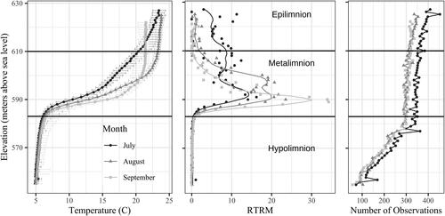
For the trend analysis, the epilimnion, metalimnion, and hypolimnion strata in the lacustrine zone were delineated based on temperature profiles, water density (computed from temperature), and relative thermal resistance to mixing (RTRM), computed from water density (Vallentyne 1957, Myers et al. 2003). Mean water density profiles were based on 1 m bins using temperature profiles from 2005 to 2020. RTRM was calculated as the change in mean density over each meter divided by the difference in water density between 5 C water and 4 C water (Vallentyne 1957, Wetzel 2001). The top and bottom elevations of the metalimnion were selected based on August RTRM values. The upper limit of the metalimnion was defined as the elevation where RTRM values began to increase from relatively low, consistent values. The lower limit of the metalimnion (upper limit of the hypolimnion) was defined as the elevation where RTRM values returned to consistent, relatively low values (Fig. 3). The downstream boundary of the transition zone was delineated based on the location where the upper limit of the hypolimnion intersected with the bottom of the reservoir (river mile 308, 496 river km, Fig. 2).

Figure 3. Brownlee Reservoir lacustrine zone median temperature (C) and relative thermal resistance to mixing (RTRM) based on 1 m bins during Jul, Aug, and Sep, over the 2005–2020 period. Temperature error bars show the interquartile range. RTRM was computed based on median temperature for each 1 m bin. Smooth vertical lines for RTRM are LOWESS lines.

In-reservoir volume-weighted DO

The profile data were summarized as volume-weighted mean DO concentration (VWDO), volume-weighted mean temperature (VWT), and anoxic volume in the transition zone, and in the epilimnion, metalimnion, and hypolimnion strata of the lacustrine zone, for each day of profiling. DO and temperature profile data were interpolated, using the inverse distance interpolation method in Tecplot 360 software, into a volumetric grid developed using measured bathymetry of Brownlee Reservoir (Berger and Wells 2021). The grid cells only included the mainstem portion of the reservoir and were 500 m long and 1.0 m deep, while cell widths were variable based on the bathymetry. VWDO and VWT in the transition zone, epilimnion, metalimnion, and hypolimnion were calculated as (1) $$\text{VWDO}\mathrm{ }\text{or}\mathrm{ }\text{VWT}=\Sigma (\text{DO}\mathrm{ }\text{or}\mathrm{ }\text{temperature}\times \text{volume})/\Sigma \mathrm{ }\text{volume}$$(1) where VWDO or VWT is the volume-weighted mean DO or temperature, DO or temperature is the interpolated profile DO or temperature for each grid cell, and volume is the volume for each grid cell.

Anoxic volume was calculated by summing the volume of each grid cell that had an interpolated DO <1 mg/L.

Trend analysis of concentrations and loads

Trends were evaluated using weighted regressions of concentrations on time, discharge, and season (WRTDS; Hirsch et al. 2010, Hirsch and De Cicco 2015). The WRTDS analyses were implemented using the Exploration and Graphics for RivEr Trends (EGRET) package within the R statistical program (R Core Team 2021). Inputs to the WRTDS model include measured concentrations and daily mean streamflow or rolling mean streamflow for reservoir DO (Supplementary material, Table S4). The multivariate regressions in WRTDS are weighted and moving based on “window” settings for each variable (time, discharge, and season) and produce estimated daily concentrations that are used to compute loads based on measured daily streamflow. For reservoir DO, multiple WRTDS models were run for the transition zone and the epilimnion, metalimnion, and hypolimnion strata using rolling mean streamflow of different periods (10, 20, 40, 60, 80, 100, 120, 140, 170, and 200 d rolling means), and the best fit model was selected based on R² between measured and modeled DO, within an expected range of residence time for the transition zone or strata (Supplementary material, Table S4). WRTDS also incorporates flow normalization that utilizes the estimated daily concentrations and filters out the influence of year-to-year variability in streamflow on trends in concentration and loads (Hirsch and De Cicco 2015). Kalman filtering (Kalman), which utilizes the actual measured concentrations on sampled days as opposed to the daily estimates, was also utilized (Hirsch 2019, Zhang and Hirsch 2019). WRTDS flow-normalized results were used to describe trends, while Kalman results were used for correlations between inflow parameters and reservoir DO.

WRTDS was run on the entire year-round datasets, and flow-normalized concentrations, Kalman concentrations, and loads were summarized for periods of interest. For inflow parameters, means were summarized for May–September (SR-HC TMDL period trends), May–August (for correlations), spring (Mar–May), summer (Jun–Aug), autumn (Sep–Nov), and winter (Dec–Feb). For VWDO in the transition zone, epilimnion, metalimnion, and hypolimnion, means were summarized for July–September (trends) and August (correlations). For anoxic volume, WRTDS was run on a combined dataset for the entire reservoir (anoxic volume of the entire reservoir), and results were also summarized for July–September and August. For years when no data were available over these summary periods, the Kalman results were not used.

The uncertainty in the WRTDS trends was quantified using block bootstrap replicates implemented using the EGRETci package in R (Hirsch et al. 2015). The default settings from Hirsch and De Cicco (2018) of a maximum and minimum number of bootstrap replicates of 100 and 40, respectively, and a block length of 200 d were used. The block bootstrap approach was used for the entire 1995–2021 timeframe and also 1995–2005 (prior to approval of the SR-HC TMDL) and 2005–2021 (after approval of the SR-HC TMDL).

The EGRET package and extensions were also utilized to screen the streamflow record for trends over the study period to understand the potential interaction between long-term streamflow trends over the study period (as opposed to interannual variability) and trends in water quality (Hirsch and De Cicco 2018). Using the EGRET package and extensions to the package (Hirsch 2018), the results of 365 individual Mann–Kendall trends tests and Theil–Sen slopes on ordered streamflow statistics were visualized in quantile-Kendall plots to indicate significance and strength of streamflow trends (Hirsch 2018, Choquette et al. 2019).

Results

Trends in streamflow, Chl-a, TSS, and nutrients

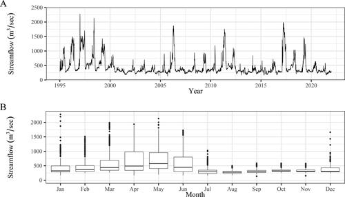
Snake River streamflow into Brownlee Reservoir typically peaked in mid to late spring following snowmelt in the mountains. Streamflow dropped quickly in July, with the lowest flows in midsummer (Fig. 4). Streamflow in autumn was typically stable through November. A series of higher water years occurred in the beginning (1995–1999) and the end (2017–2019) of the trend period (Fig. 4). Trends in streamflow over the May–September SR-HC TMDL period (1995–2021) were modestly decreasing (Theil–Sen slopes of about −1% per year) and nonsignificant (P > 0.1) except for the very lowest flows (Supplementary material, Fig. S1).

Figure 4. Daily mean Snake River streamflow (m³/sec) from 1995 to 2021 (Panel A, USGS Snake River at Weiser gauge number 13269000) and box plots of daily mean streamflow from 1995 to 2021 grouped by month (Panel B). The top and the bottom of the boxes show the 75% and 25% percentiles, respectively, the whiskers extend to 1.5 times the interquartile range, and points show outliers.

Measured concentrations input to WRTDS showed high inter- and intra-annual variability (Supplementary material, Figs. S2 and S3). WRTDS models produced reasonable estimated daily concentrations (Hirsch and De Cicco 2015, Supplementary material, Fig. S4, Table S4). Flow-normalized concentrations of Chl-a, TSS, and TP significantly decreased from 1995 to 2021 (P < 0.05), while trends in TN were not significant (P = 0.46, Fig. 5). Flow-normalized concentrations of Chl-a, TSS, and TP decreased 80%, 61%, and 46%, respectively, from 1995 to 2021 (Table 1). In Fig. 5, the Kalman filtered estimated mean concentrations for May to September (indicated by the dots) show strong interannual variations as compared to the flow-normalized concentrations (indicated by the smooth curve). Since inflow parameters were collected frequently (generally every 2 weeks) and the WRTDS Kalman concentrations include measured data when they exist, the May–September mean Kalman concentrations agree well with measured concentrations (Supplementary material, Fig. S3, Fig. 5).

Figure 5. Mean May–Sep WRTDS flow-normalized concentration trends and Kalman concentrations for Brownlee Reservoir inflowing Chl-a, TSS, and nutrients from 1995 to 2021. P-values are from block bootstrap tests on flow-normalized concentrations.

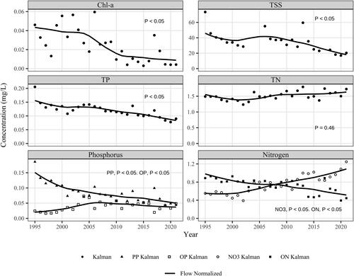
Comparing 1995–2005 and 2005–2021 showed that the strength of trends for Chl-a, TP, TN, and TSS changed around 2005 (Table 1). Block bootstrap tests reflected this change, with trends in Chl-a, TP, TN, and TSS changing from not significant (P > 0.1) over the 1995–2005 period to significant (P < 0.05) over the 2005–2021 period (Table 1). The relatively stable TP condition over the 1995–2005 period is likely a net result of significant (P < 0.05) contradictory trends in PP and OP (decreasing PP and increasing OP, Table 1, Fig. 5, phosphorus). After 2005, only the PP component was significantly decreasing (P < 0.05; Table 1). Contradictory trends in the components of TN (increasing NO₃ and decreasing ON) occurred over the entire timeframe for the net result of no trend in TN from 1995 to 2021. However, significant increases in TN were seen from 2005 to 2021 even with the contradictory directions of NO₃ and ON trends due to the increases in NO₃ (65% from 2005 to 2021, Fig. 5, Table 1).

Trends in flow-normalized loads of Chl-a, TP, TN, and TSS followed the trends in concentrations, with no significant trends seen from 1995 to 2005, and significant decreases (P < 0.05), in Chl-a (69%), TP (36%), and TSS (60%) from 2005 to 2021 (Table 1). The components of TP load, similar to concentration, showed contradictory trends from 1995 to 2005 (increasing OP and decreasing PP loads), while from 2005 to 2021 only the PP loads showed significant decreases (P < 0.05; Table 1). Again, similar to concentration, NO₃ loads increased significantly (P < 0.05), and strongly (64% increase) from 2005 to 2021 (Table 1).

Trends in Chl-a and nutrients during other seasons

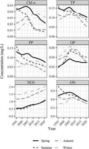
The May–September period ignores potential trends during times when the highest concentrations can occur. For example, annual peaks in Chl-a typically occurred in early spring, prior to May (Mar 2004, measured peak of 0.176 mg/L), and winter concentrations were also high, with peaks in January and February exceeding 0.08 mg/L in some years (Supplementary material, Table S1). Trends in flow-normalized Chl-a concentrations during spring, summer, and autumn were decreasing, consistent with the May–September trends. However, winter Chl-a concentrations increased nearly 4-fold over the 27 years (Fig. 6). TP decreased in all seasons, with relatively large decreases in autumn and winter from 2012 to 2021 that coincided with similar decreases in OP, but not PP (Fig. 6). NO₃ increased in all seasons, with the largest increases in autumn and winter, when concentrations were highest, compared to spring and summer, when concentrations were lower (Fig. 6).

Figure 6. Mean WRTDS flow-normalized concentrations of Chl-a, TP, OP, PP, NO₃, and ON during spring (Mar–May), summer (Jun–Aug), autumn (Sep–Nov), and winter (Dec–Feb).

Patterns in reservoir DO

The lowest levels of VWDO occurred during July in the transition zone, during August in the epilimnion and metalimnion, and during September in the hypolimnion (Fig. 7). Hypolimnion VWDO eventually approached zero in every year but there was some notable variability. VWDO showed 2 outliers (2001 and 2014) with August hypolimnion VWDO of 1.3 and 1.2 mg/L, respectively, compared to the median of 0.4 mg/L over all the years. These 2 years were also the hypolimnion VWDO outliers in September (Fig. 7). The slightly higher hypolimnion VWDO in these 2 years may relate to a slightly colder hypolimnion with August VWT of 4.8 C (2014), compared to median VWT of 5.5 C (Fig. 7). Variability in hypolimnion VWDO in October and November is related to the timing of plunging inflows, mixing, and recovery of DO, which can occur in late October and November in high water years (Figs. 2 and 7, Supplement A, 2017). Outlier points throughout the year for hypolimnion VWT are these high water years (1998, 2006, 2011, and 2017) when the hypolimnion VWT was warmer (>10 C), as opposed to near 5 C. Anoxic volume peaked in the metalimnion in August, while the hypolimnion gradually built up anoxia until nearly complete anoxia in September. Similar to VWDO, 2001 and 2014 were also outlier points with low hypolimnetic anoxic volume (Fig. 7).

Figure 7. Box plots of monthly measured volume-weighted dissolved oxygen (VWDO [mg/L]), volume-weighted temperature (VWT [C]), and anoxic volume (million m³) in the transition zone, epilimnion, metalimnion, and hypolimnion of Brownlee Reservoir. Plots include all measured data used in WRTDS modeling from 1995 to 2021. Numbers at the top of the top panel indicate number of individual profiling dates available for the month. The top and the bottom of the boxes show the 75% and 25% percentiles, respectively, the whiskers extend to 1.5 times the interquartile range, and points show outliers.

WRTDS trends in reservoir DO

WRTDS was effective at estimating VWDO in the transition zone and in the epilimnion, metalimnion, and hypolimnion strata of the lacustrine zone, and anoxic volume for the entire reservoir (Supplementary material, Table S4, Figs. S5 and S6). The good fit of the WRTDS models (Supplementary material, Fig. S5) indicates streamflow-related mixing of inflows and seasonal thermal stratification are key drivers of DO conditions in Brownlee Reservoir. Mean July–September flow-normalized VWDO increased significantly (P < 0.05) for the transition zone, epilimnion, and metalimnion over the entire time period and before and after approval of the SR-HC TMDL (Fig. 8, Table 2). There were no significant trends for the hypolimnion over any of the time periods. Metalimnion VWDO improved 115% (1.7 mg/L) since 1998, while epilimnion VWDO improved 53% (2.5 mg/L). Trends from the beginning of the period to 2005 are less reliable than trends after 2005 because VWDO calculations can be sensitive to the resolution and coverage of the measured profile data (Quinlan et al. 2005), which was less extensive during the early period. The resolution of the profiling since 2005 has been relatively consistent spatially and temporally, and coverage has been more extensive with use of the SBE-19plus. Since 2005, July–September mean transition zone, epilimnion, and metalimnion flow-normalized VWDO improved by 1.0, 1.6 and 1.1 mg/L, respectively, and the Anoxic Volume for the entire reservoir has improved by 33% (Fig. 8, Table 2).

Figure 8. Panel A: Trends in mean Jul–Sep WRTDS flow-normalized volume-weighted dissolved oxygen (VWDO [mg/l]) in the transition zone (1995–2021), epilimnion (1998–2021), metalimnion (1998–2021), and hypolimnion (1998–2021). Panel B: Trends in WRTDS flow-normalized anoxic volume in the entire reservoir (million m³), over Jul–Aug and Aug. In both panels, the dots are Kalman filtered estimated mean concentrations and the smooth curves are mean WRTDS flow-normalized concentrations. P-values are from block bootstrap tests on flow-normalized concentrations.

Inflowing parameters related to in-reservoir DO

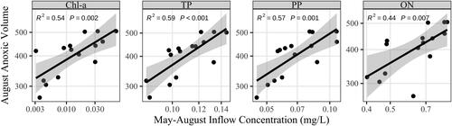
August VWDO in the transition zone, epilimnion, and metalimnion and anoxic volume in the entire reservoir showed multiple significant (P < 0.05) correlations with inflowing parameters (Fig. 9). Hypolimnion VWDO showed no significant correlations with any of the inflow parameters (Fig. 9). Inflow Chl-a was also significantly (P < 0.05) related to most of the nutrient parameters, and TSS, either positively (particulate nutrient fractions and TSS) or negatively (dissolved fractions) in a pattern consistent with increasing dissolved nutrient uptake with increasing Chl-a concentrations (Fig. 9). Epilimnion VWDO decreased (R² > 0.65, P < 0.001) with increasing inflowing Chl-a, TP, PP, and ON. Metalimnion VWDO relationships showed patterns similar to the epilimnion but were not as strong (Fig. 10). Transition zone VWDO only showed a significant relationship with TP over the May–August period (Fig. 10); however, inflow Chl-a during April and May was also significantly (P < 0.05) correlated with transition-zone VWDO (Supplementary material, Fig. S7). Anoxic volume increased with increasing Chl-a, TP, PP, and ON (Fig. 11).

Figure 9. Correlation matrix of mean Kalman May–Aug inflow Chl-a, TSS, and nutrient concentrations, mean Aug Kalman volume-weighted dissolved oxygen (VWDO) in the transition zone, epilimnion, metalimnion, and hypolimnion of Brownlee Reservoir, and anoxic volume in the entire reservoir. Correlations were limited to the years 2005–2021 due to reservoir DO profile data availability and coverage. Labels in the boxes are significant (P < 0.05) Pearson’s correlation coefficients on log10 transformed values, and blank boxes indicate the correlation was not significant (P > 0.05).

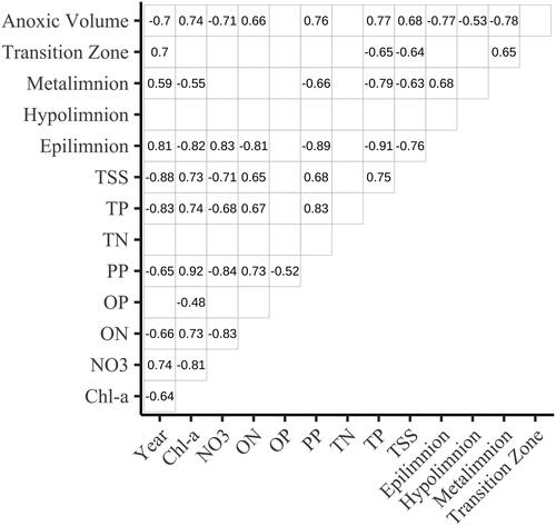
Figure 10. Regressions between inflowing Kalman Chl-a, TP, PP, and ON (mean, May–Aug) and Kalman volume-weighted dissolved oxygen (VWDO) in the transition zone, epilimnion, and metalimnion (mean, Aug) during the 2005–2021 time period. R² and P values are linear regression statistics on log10 transformed values.

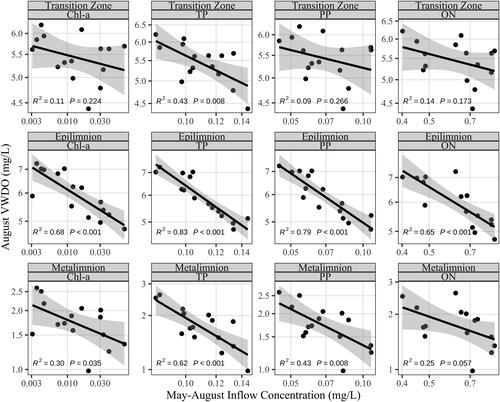
Figure 11. Regressions between inflowing Kalman Chl-a, TP, PP, and ON (mean, May–Aug) and mean Kalman anoxic volume in Aug (million m³) in the entire reservoir. R² and P values are linear regression statistics on log10 transformed values.

Discussion

Inflow trends

The SR-HC TMDL targeted a 54% decrease in TP load at Brownlee Reservoir inflow (IDEQ and ODEQ 2004). Since then, TP has shown a 37% reduction in flow-normalized concentrations and a 36% reduction in flow-normalized loads (Table 1). Decreasing TP trends are not limited to the Snake River immediately upstream of Brownlee Reservoir and were also seen 200 miles (322 km) upstream from Brownlee Reservoir at King Hill, Idaho, from efforts associated with the middle Snake River and upper Snake-Rock TMDLs approved in 1997 (Maret et al. 2008, Tetra Tech 2014, IDEQ 2021). PP at the inflow to Brownlee Reservoir showed a 43% decrease prior to SR-HC TMDL approval, which may be related to these efforts far upstream focused on best management practices (BMPs) relative to irrigated agriculture such as settling ponds and conversion from flood to sprinkler (Bjorneberg et al. 2015). Relatively steep decreases in OP in autumn and winter since 2015 may be indicative of OP-focused reductions, especially when considering contributions to the Snake River from the Boise River, where OP is a relatively large phosphorus contribution in autumn and winter when irrigation season has ended (MacCoy 2004, Wood and Etheridge 2011, USGS 2022). Average TP concentrations at the mouth of the Boise River from September to December decreased approximately 36% from 2015 to 2021, during which TP was approximately 75% OP (Supplementary material, Table S5; USGS 2022).

Increasing Snake River NO₃ trends during autumn and winter, similar to decreasing phosphorus trends, were not unique to Brownlee Reservoir inflow. Increasing NO₃ trends occurred upstream of King Hill, Idaho (Jerome, Gooding, and Twin Falls counties), in groundwater well networks, agricultural field drains, and springs returning to the Snake River (Franz et al. 2012, Tetra Tech 2014, Bjorneberg et al. 2020). Lentz et al. (2018) and Franz et al. (2012) associated the NO₃ increase in the shallow groundwater system to changes in agricultural practices. Similar changes in agricultural practices have occurred statewide throughout Idaho (USDA 2021).

The SR-HC TMDL used Chl-a as a surrogate for algal biomass and set Chl-a and TP targets that were intended to improve conditions relative to recreational use and aesthetics upstream of Brownlee Reservoir by reducing TP and nuisance algae. In turn, these reduced Chl-a and TP levels upstream of Brownlee Reservoir were expected to reduce phosphorus and organic matter delivery to Brownlee Reservoir and thereby improve DO conditions in the reservoir. Flow-normalized trends show Chl-a has indeed decreased along with TP since 2005; however, TP has declined relatively steadily over the years, while Chl-a declined quickly from approximately 2005 to 2010 and then leveled off (Fig. 5). Nutrient supply to the river upstream of Brownlee Reservoir has changed over the years. However, the interaction of the many controls on suspended algal biomass (nutrient supply, light availability, flow/scouring) in the Snake River is not well understood or studied. It is likely that a combination of factors contributes to the decline in Chl-a. Relative to nutrient supply, OP concentrations remain relatively high (median OP concentrations near 0.03 mg/L in recent years, Supplementary material, Fig. S3), and NO₃ has been increasing, suggesting there is still adequate nutrient supply for production of suspended algae (Reynolds and Davies 2001, Chorus and Spijkerman 2021). Light availability in the wide, shallow river upstream should be improving with the decreasing trend in TSS, which could promote suspended algae. Conversely, relative to flow/scouring, declines in summer streamflow could result in less benthic algal biomass being resuspended and more suspended algae settling, decreasing suspended algae (Worth 1995, MacCoy 2004). Despite the lack of documentation regarding the range of processes potentially controlling algal production and transport in the Snake River upstream of Brownlee Reservoir, this study documents that Chl-a and TP concentrations in the Snake River have declined over the years.

DO trends and correlations with inflow

Low DO conditions in Brownlee Reservoir, as in many reservoirs, are dynamic and are generally driven by decomposition and respiration of organic matter (Wetzel 2001). Organic matter (living or dead) can originate in the upstream river and be delivered by inflowing water to specific zones or strata in the reservoir via hydrodynamic interflows or density currents (Thornton et al. 1990, Welch et al. 2015) or be produced within the reservoir and settle through the water column. Low DO conditions in a zone or strata can also be caused by hydrodynamic transport of low DO water (and associated reduced materials) from upstream anoxic areas via the same density currents (Thornton et al. 1990, Baldwin et al. 2022). The contrast in Brownlee Reservoir between improving VWDO in the transition zone, epilimnion, and metalimnion and no trends in the hypolimnion suggests a close connection of the transition zone, epilimnion, and metalimnion to inflowing organic matter. Lack of improvement in the hypolimnion suggests it may be more closely connected to other factors, such as in-reservoir produced organic matter (commonly expressed as large cyanobacterial blooms; Myers et al. 2003), sediment-related oxygen demand from previously captured materials (Matzinger et al. 2010), and/or hydrodynamics of the system. Relative to in-reservoir productivity, the lack of hypolimnetic DO trends may be related to in-reservoir productivity not yet responding to reduced phosphorus supply and/or internal phosphorus recycling providing sufficient phosphorus to support in-reservoir productivity. Perhaps inflow TP reductions have not yet been large enough to affect in-reservoir productivity, especially considering that in-reservoir productivity may not respond to TP reductions until some threshold value is reached (Carvalho et al. 2013, Schindler et al. 2016). Potential threshold levels are highly site specific and have not been evaluated for Brownlee Reservoir, but general ranges based on cyanobacterial blooms in more than 800 European lakes (Carvalho et al. 2013) and review of phosphorus levels that may limit either uptake rates or overall phytoplankton biomass (Reynolds and Davies 2001, Chorus and Spijkerman 2021) are more than 50% lower for OP and approximately 30% lower for TP compared to current levels in Brownlee Reservoir.

Many long-term case histories document recovery from eutrophication in lakes following reductions of TP inputs (Jeppesen et al. 2005, Schindler et al. 2016). Some studies have used improvements in DO to evaluate recovery (Matthews and Effler 2006, Matthews et al. 2015). However, many of these studies focus only on hypolimnetic DO (Li et al. 2018, Nelligan et al. 2019). While case studies for DO responses to TP load reductions in large mainstem reservoirs are not common, Welch et al. (2015) documented recovery of DO in the hypolimnion of a relatively small (approximately 20% the volume of Brownlee Reservoir but with similar residence time) mainstem reservoir (Lake Spokane, Washington) following input TP reductions from wastewater treatment. They documented a relatively quick recovery compared to lakes, and attributed the quick recovery to high inflow and short residence times. Cooke et al. (2011) documented the reverse case (Tenkiller Reservoir, OK) where inflow TP more than doubled from nonpoint animal agriculture and reservoir hypolimnetic DO responded in step with a more than double decline in oxygen conditions (expressed as the areal hypolimnetic oxygen deficit, AHOD). In both reservoir cases the relative magnitudes of the TP decreases (or increases) and hypolimnetic DO increases (or decreases) were comparable where an 80% decrease or 140% increase in TP resulted in approximately 80% increase or 140% decrease in AHOD (Cooke et al. 2011, Welch et al. 2015). While this study used anoxic volume rather than AHOD as a metric for anoxia, we also found a relationship close to 1:1 between the change in TP and anoxic volume. Specifically, a 36% reduction in TP corresponded to a 33% reduction of anoxic volume (Tables 1 and 2). Brownlee Reservoir DO improvements have also been quick, with inflow concentrations in a given year correlated with DO conditions within that same year. However, this study documented a unique situation, compared to these 2 reference case studies, where the hypolimnetic DO has not responded.

In the 2 referenced reservoir case studies, the response of the reservoir to a changing TP supply was assessed by hypolimnetic DO conditions responding to changes in reservoir trophic state, primary productivity, and in-reservoir produced organic matter settling to the hypolimnion and decomposing (Cooke et al. 2011, Welch et al. 2015). Inflowing Chl-a or organic matter conditions were not evaluated relative to DO conditions. However, other reservoir studies have linked inflowing organic matter to oxygen demand in the reservoir. Marcé et al. (2008) found that epilimnion nutrient and Chl-a concentrations were not correlated with hypolimnetic oxygen demand; rather, inflow dissolved organic carbon was strongly correlated because inflowing water plunged to the hypolimnion via density currents. In Brownlee Reservoir, in most years, the inflow water does not plunge into the hypolimnion until very late in the season (Supplement A), potentially explaining why inflow organic matter reductions show no correlation with hypolimnetic DO during summer months within Brownlee Reservoir, as was found by Marcé et al. (2008). In Brownlee Reservoir, water flowing into the reservoir flows through the transition zone and interflows into the epilimnion and metalimnion throughout the summer and autumn, delivering inflow organic matter directly to these strata where settling and decomposition has a direct and immediate effect on DO.

Botelho and Imberger (2007) evaluated the connection between inflow organic matter and transition zone DO during their study of the “DO block” in Brownlee Reservoir. The DO block can occur where very low DO conditions (1.0–3.0 mg/L) develop within 5–10 miles (8–16 km) of the transition zone through the entire vertical water column in midsummer (Ebel and Koski 1968, Cole and Hannan 1990, Botelho and Imberger 2007). In this study, this condition was observed in the early 2000s (Supplementary material, Fig. S5, Panel A, transition zone) and was even more extreme in the early 1990s (Myers et al. 2003). However, the DO block has not been observed since 2005, and midsummer VWDO in the transition zone has not fallen below 4 mg/L. Botelho and Imberger (2007) determined that the DO block resulted from specific hydrodynamic and meteorological conditions, combined with inflowing organic matter, that created a convergence zone where the residence time was long enough to reduce DO through the entire water column, as opposed to upwelling of deeper anoxic water from internal wave action. A portion of the oxygen demand was from the settling, respiration, and decomposition of the diatom-dominated inflow phytoplankton community, as supported by Chl-a measurements that decreased moving downstream through the transition zone (Myers et al. 2003, Botelho and Imberger 2007). In this study, inflow concentrations of Chl-a were correlated with VWDO in the transition zone; however, correlations showed that inflow Chl-a concentrations in April and May were more significantly related to August VWDO in the transition zone than July and August. This suggests that spring diatom blooms, settling and decomposing in the transition zone, are important for transition-zone DO (Supplementary material, Fig. S7). The lack of strong correlations between transition-zone VWDO and July or August inflow Chl-a supports a conclusion that low midsummer inflow Chl-a in recent years (Fig. 6) is no longer high enough to cause a DO block condition in most of the years of the dataset used for the correlations (2005–2021).

The trends and correlations in this study support a primary premise of the SR-HC TMDL that TP and Chl-a reductions in the river inflow to Brownlee Reservoir would improve DO conditions within the reservoir. The reduced inflow of particulate organic material and not dissolved nutrients seems to be the primary driver of the improved DO thus far. The OP component of TP has not changed significantly since 2005, remaining relatively high, and there has been an unanticipated (by the SR-HC TMDL) increase in NO₃. While reduced inflow of particulate organic material has improved DO conditions in the transition zone, epilimnion, and metalimnion, it is possible that the dissolved nutrients not changing (or increasing) is maintaining in-reservoir productivity to a point where DO in the hypolimnion has not shown a response. The DO improvement in the transition zone, epilimnion, and metalimnion has been very rapid in response to inflow reductions. Overall, this study highlights the usefulness of long-term monitoring programs to provide empirical support to management decisions, specifically supporting the reduction of Brownlee Reservoir inflow TP as an effective but incomplete way to quickly improve Brownlee Reservoir DO conditions and suggesting that further improvements from inflow reductions may be possible.

Acknowledgements

The development of this 27 yr dataset would not have been possible without the participation and support of many Idaho Power personnel, including the ongoing support of Brett Dumas and Jim Chandler and the field efforts of Jim Younk. Jack Harrison (HyQual) contributed significant early analysis of Snake River organic matter and Brownlee Reservoir dissolved oxygen and provided ongoing encouragement. Several USGS personnel also contributed ongoing support, ideas, and review of this study. Specifically, thanks to Bob Hirsch, who provided much needed guidance on the WRTDS modeling and actual R code needed to facilitate the reservoir DO WRTDS modeling. Thanks go to others at the USGS for supporting this work as an important component of an ongoing USGS study of mercury dynamics in the Hells Canyon Complex reservoirs: Dave Krabbenhoft, Austin Baldwin, Mike Tate, Collin Eagles-Smith, James Willacker, Mark Marvin-DePasquale, Amy Yoder, and also Brett Poulin (University of California, Davis) and Greg Clark (USGS, retired).

References

- Baldwin AK, Eagles-Smith CA, Willacker JJ, Poulin BA, Krabbenhoft DP, Naymik J, Tate MT, Bates D, Gastelecutto N, Hoovestol C, Larsen C, et al. 2022. In-reservoir physical processes modulate aqueous and biological methylmercury export from a seasonally anoxic reservoir. Environ Sci Technol. 56(19):13751–13760. doi:10.1021/acs.est.2c03958.
- Baldwin AK, Poulin BA, Naymik J, Hoovestol C, Clark GM, Krabbenhoft DP. 2020. Seasonal dynamics and interannual variability in mercury concentrations and loads through a three-reservoir complex. Environ Sci Technol. 54(15):9305–9314. doi:10.1021/acs.est.9b07103.
- Berger CJ, Wells SA. 2021. Draft. Hells Canyon Complex CE-QUAL-W2 model development and calibration. Portland (OR): Water Quality Research Group. Portland State University; 193 p.
- Bjorneberg DL, Ippolito JA, King BA, Nouwakpo SK, Koehn AC. 2020. Moving toward sustainable irrigation in a southern Idaho irrigation project. Trans Am Soc Agric Biol Eng. 63(5):1441–1449. doi:10.13031/trans.13955.
- Bjorneberg DL, Leytem AB, Ippolito JA, Koehn AC. 2015. Phosphorus losses from an irrigated watershed in the Northwestern United States: case study of the Upper Snake Rock watershed. J Environ Qual. 44(2):552–559. doi:10.2134/jeq2014.04.0166.
- Botelho DA, Imberger J. 2007. Dissolved oxygen response to wind-inflow interactions in a stratified reservoir. Limnol Oceanogr. 52(5):2027–2052. doi:10.4319/lo.2007.52.5.2027.
- Carvalho L, McDonald C, de Hoyos C, Mischke U, Phillips G, Borics G, Poikane S, Skjelbred B, Solheim AL, Van Wichelen J, et al. 2013. Sustaining recreational quality of European lakes: minimizing the health risks from algal blooms through phosphorus control. J Appl Ecol. 50(2):315–323. doi:10.1111/1365-2664.12059.
- Choquette AF, Hirsch RM, Murphy JC, Johnson LT, Confesor RB, Jr. 2019. Tracking changes in nutrient delivery to western Lake Erie: approaches to compensate for variability and trends in streamflow. J Great Lakes Res. 45(1):21–39. doi:10.1016/j.jglr.2018.11.012.
- Chorus I, Spijkerman E. 2021. What Colin Reynolds could tell us about nutrient limitation, N:P rations and eutrophication control. Hydrobiologia. 848(1):95–111. doi:10.1007/s10750-020-04377-w.
- Clark GM, Naymik J, Krabbenhoft DP, Eagles-Smith CA, Aiken GR, Marvin-DiPasquale MC, Harris RC, Myers R. 2016. Mercury cycling in the Hells Canyon Complex of the Snake River, Idaho and Oregon. Fact Sheet; USGS Numbered Series 2016-3051. Reston (VA): U.S. Geological Survey; 6 p.
- Cole TM, Hannan HH. 1990. Dissolved oxygen dynamics. In: Thornton KW, Kimmel BL, Payne FE, editors. Reservoir limnology: ecological perspectives. New York (NY): John Wiley and Sons; p. 71–107.
- Cooke GD, Welch EB, Jones JR. 2011. Eutrophication of Tenkiller Reservoir, Oklahoma, from nonpoint agricultural runoff. Lake Reserv Manag. 27(3):256–270. doi:10.1080/07438141.2011.607552.
- Ebel WL, Koski CH. 1968. Physical and chemical limnology of Brownlee Reservoir, 1962–64. Fishery Bulletin. US Fish Wildlife Service. 67(2):295–335.
- Franz LM, Rupert MG, Hunt CD, Jr, Skinner KD. 2012. Groundwater quality in the Columbia Plateau, Snake River Plain, and Oahu Basaltic-Rock and Basin-Fill Aquifers in the Northwestern United States and Hawaii, 1992-2010. Reston (VA): National Water-Quality Assessment Program. U.S. Geological Survey Scientific Investigations Report 2012–5123.
- Hirsch RM. 2018. Daily streamflow trend analysis. U.S. Geological Survey Office of Water Information Blog; [cited 2021 Oct 26]. https://waterdata.usgs.gov/blog/quantile-kendall/.
- Hirsch RM. 2019. Making WRTDS_K flux estimates: U.S. Geological Survey Exploration and Graphics for RivEr Trends (EGRET); [cited 4 Nov 2020]. Available from http://usgs-r.github.io/EGRET/articles/Making%20WRTDS_K%20flux%20estimates.html.
- Hirsch RM, Archfield SA, De Cicco LA. 2015. A bootstrap method for estimating uncertainty of water quality trends. Environ Model Softw. 73:148–166. doi:10.1016/j.envsoft.2015.07.017.
- Hirsch RM, De Cicco LA. 2015. User guide to Exploration and Graphics for RivEr Trends (EGRET) and dataRetrieval: R packages for hydrologic data (version 2.0, Feb 2015): U.S. Geological Survey Techniques and Methods 4-A10; 104 p.
- Hirsch RM, De Cicco LA. 2018. Guide to EGRET 3.0 enhancements: U.S. Geological Survey Exploration and Graphics for RivEr Trends (EGRET); [cited 8 Aug 2020]. Available from http://usgs-r.github.io/EGRET/articles/Enhancements.html.
- Hirsch RM, Moyer DL, Archfield SA. 2010. Weighted regressions on time, discharge, and season (WRTDS), with an application to Chesapeake Bay river inputs. J Am Water Resour Assoc. 46(5):857–880. doi:10.1111/j.1752-1688.2010.00482.x.
- [IDEQ] Idaho Department of Environmental Quality. 2021. Snake River (Upper Snake-Rock) Subbasin; [cited 4 Nov 2021]. Available from https://www.deq.idaho.gov/water-quality/surface-water/total-maximum-daily-loads/snake-river-upper-snake-rock-subbasin/.
- [IDEQ and ODEQ] Idaho Department of Environmental Quality, Oregon Department of Environmental Quality. 2004. Snake River-Hells Canyon total maximum daily load. IDEQ Boise Regional Office and ODEQ Pendleton Office; [cited 4 Nov 2020]. Available from https://www.deq.idaho.gov/water-quality/surface-water/total-maximum-daily-loads/snake-river-hells-canyon-subbasins/.
- Jeppesen ERIK, Sondergaard M, Jensen JP, Havens KE, Anneville O, Carvalho L, Coveney MF, Deneke R, Dokulil MT, Foy BOB, et al. 2005. Lake responses to reduced nutrient loading – an analysis of contemporary long-term data from 35 case studies. Freshwater Biol. 50(10):1747–1771. doi:10.1111/j.1365-2427.2005.01415.x.
- Kimmel BL, Groeger AW. 1984. Factors controlling primary production in lakes and reservoirs: a perspective. Lake Reserv Manage. 1(1):277–281. doi:10.1080/07438148409354524.
- Lentz RD, Carter DL, Haye SV. 2018. Changes in groundwater quality and agriculture in forty years on the Twin Falls irrigation tract in southern Idaho. J Soil Water Conserv. 73(2):107–119. doi:10.2489/jswc.73.2.107.
- Li J, Molot LA, Palmer ME, Winter JG, Young JD, Stainsby EA. 2018. Long-term changes in hypolimnetic dissolved oxygen in a large lake: effects of invasive mussels, eutrophication and climate change on Lake Simcoe, 1980–2012. J Great Lakes Res. 44(4):779–787. doi:10.1016/j.jglr.2018.05.016.
- MacCoy DE. 2004. Water-quality and biological conditions in the lower Boise River, Ada and Canyon counties, Idaho, 1994-2002. U.S. Geological Survey Scientific Investigations Report 2004–5128.
- Marcé R, Moreno-Ostos E, Armengol J. 2008. The role of river inputs on the hypolimnetic chemistry of a productive reservoir: implications for management of anoxia and total phosphorus internal loading. Lake Reserv Manage. 24(1):87–98. doi:10.1080/07438140809354053.
- Maret TR, MacCoy DE, Carlisle DM. 2008. Long-term water quality and biological responses to multiple best management practices in Rock Creek, Idaho. J Am Water Resour Assoc. 44(5):1248–1269. doi:10.1111/j.1752-1688.2008.00221.x.
- Matthews DA, Effler SW. 2006. Assessment of long-term trends in the oxygen resources of a recovering urban lake, Onondaga Lake, New York. Lake Reserv Manage. 22(1):19–32. doi:10.1080/07438140609353881.
- Matthews D, Effler S, Prestigiacomo A, O’Donnell S. 2015. Trophic state responses of Onondaga Lake, New York, to reductions in phosphorus loading from advanced wastewater treatment. IW. 5(2):125–138. doi:10.5268/IW-5.2.756.
- Matzinger A, Müller B, Niederhauser P, Schmid M, Wüest A. 2010. Hypolimnetic oxygen consumption by sediment-based reduced substances in former eutrophic lakes. Limnol Oceanogr. 55(5):2073–2084. doi:10.4319/lo.2010.55.5.2073.
- Myers R, Harrison J, Parkinson SK, Hoelscher B, Naymik J, Parkinson SE. 2003. Pollutant transport and processing in the Hells Canyon Complex. Boise (ID): Idaho Power Company. In: Technical appendices for new license application: Hells Canyon Hydroelectric Complex. Technical Report E.2.2-2.
- Nelligan C, Jeziorski A, Rühland KM, Paterson AM, Smol JP. 2019. Long-term trends in hypolimnetic volumes and dissolved oxygen concentrations in Boreal Shield lakes of south-central Ontario, Canada. Can J Fish Aquat Sci. 76(12):2315–2325. doi:10.1139/cjfas-2018-0278.
- Nürnberg GK. 1995. Quantifying anoxia in lakes. Limnol Oceanogr. 40(6):1100–1111. doi:10.4319/lo.1995.40.6.1100.
- Nürnberg GK. 2002. Quantification of oxygen depletion in lakes and reservoirs with the hypoxic factor. Lake Reserv Manage. 18(4):299–306. doi:10.1080/07438140209353936.
- Quinlan R, Paterson AM, Smol JP, Douglas MSV, Clark BJ. 2005. Comparing different methods of calculating volume weighted hypolimnetic oxygen (VWHO) in lakes. Aquat Sci. 67(1):97–103. doi:10.1007/s00027-004-0717-6.
- R Core Team. 2021. R: a language and environment for statistical computing. Vienna (Austria): R Foundation for Statistical Computing. https://www.R-project.org/.
- Reynolds CS, Davies PS. 2001. Sources and bioavailability of phosphorus fractions in freshwaters: a British perspective. Biol Rev Camb Philos Soc. 76(1):27–64. doi:10.1017/s1464793100005625.
- Schindler DW, Carpenter SR, Chapra SC, Hecky RE, Orihel DM. 2016. Reducing phosphorus to curb lake eutrophication is a success. Environ Sci Technol. 50(17):8923–8929. doi:10.1021/acs.est.6b02204.
- Sullivan AB, Jager HI, Myers R. 2003. Modeling white sturgeon movement in a reservoir: the effect of water quality and sturgeon density. Ecol Modell. 167(1-2):97–114. doi:10.1016/S0304-3800(03)00169-8.
- Tetra Tech. 2014. Reevaluation of the Mid Snake/Upper Snake-Rock Subbasin TMDL: data summary, evaluation, and assessment. Prepared for U.S. Environmental Protection Agency. Seattle, WA; 202 p.
- Thornton KW, Kimmel BL, Payne FE, editors. 1990. Reservoir limnology: ecological perspectives. New York (NY): John Wiley and Sons; 246 p.
- [USDA] US Department of Agriculture. 2021. National Agricultural Statistics Service: Quick Stats; [cited 15 Apr 2021]. Available from https://www.nass.usda.gov/Statistics_by_State/Idaho/index.php.
- [USGS] US Geological Survey. 2022. National Water Information System data available on the World Wide Web (USGS Water Data for the Nation); [cited May 25 2022]. Available from https://waterdata.usgs.gov/nwis?.
- Vallentyne JR. 1957. The principles of modern limnology. Am Sci. 45(3):218–244.
- Welch EB, Brattebo SK, Gibbons HL, Plotnikoff RW. 2015. A dramatic recovery of Lake Spokane water quality following wastewater phosphorus reduction. Lake Reserv Manage. 31(2):157–165. doi:10.1080/10402381.2015.1040566.
- Welcker CK, Anderson K, Carson G. 2018. Fifty years of sediment dynamics in a large reservoir in the western US. Abstract G51C-0505 presented at 2018 Fall Meeting, American Geophysical Union, Washington, DC, 10-14 Dec.
- Wetzel RG. 2001. Limnology: lake and reservoir ecosystems. 3rd ed. San Diego (CA): Academic Press.
- Wood MS, Etheridge AB. 2011. Water-quality conditions near the confluence of the Snake and Boise Rivers, Canyon County, Idaho. U.S. Geological Survey Scientific Investigations Report 2011–5217.
- Worth DF. 1995. Gradient changes in water quality during low flows in run-of-the-river and reservoir impoundments, Lower Snake River, Idaho. Lake Reserv Manage. 11(3):217–224. doi:10.1080/07438149509354202.
- Zhang Q, Hirsch RM. 2019. River water-quality concentration and flux estimation can be improved by accounting for serial correlation through an autoregressive model. Water Resour Res. 55(11):9705–9723. doi:10.1029/2019WR025338.