Assessment of a common nonlinear eddy-viscosity turbulence model in capturing laminarization in mixed convection flows

ABSTRACT

Laminarization is an important topic in heat transfer and turbulence modeling. Recent studies have demonstrated that several well-known turbulence models failed to provide accurate prediction when applied to mixed convection flows with significant re-laminarization effects. One of those models, a well-validated cubic nonlinear eddy-viscosity model, was observed to miss this feature entirely. This paper studies the reasons behind this failure by providing a detailed comparison with the baseline Launder–Sharma model. The difference is attributed to the method of near-wall damping. A range of tests have been conducted and two noteworthy findings are reported for the case of flow re-laminarization.

Nomenclature

Bo	=	= buoyancy parameter, 8 × 104Gr/(Re 3.425 Pr0.8)
cf	=	= local friction coefficient
Cμ	=	= constant in eddy-viscosity models
D	=	= pipe diameter
Eϵ	=	= near-wall source term
fμ	=	= damping function
gi	=	= acceleration due to gravity
Gr	=	= Grashof number,
k	=	= turbulent kinetic energy,
Nu	=	= Nusselt number,
p	=	= pressure
Pk	=	= rate of shear-production of k,
Pr	=	= Prandtl number, cpμ/λ
	=	= wall heat flux
R	=	= pipe radius
Re	=	= Reynolds number, UbD/v
Ret	=	= turbulent Reynolds number,
S	=	= strain parameter
T	=	= temperature
T+	=	= non-dimensional temperature, (Tw–T)/Tτ
Tτ	=	= friction temperature, /ρ.cp.Uτ
U+	=	= non-dimensional velocity, U/Uτ
Uτ	=	= friction velocity,
Ui, ui	=	= mean, fluctuating velocity components in Cartesian tensors
	=	= Reynolds stress tensor
	=	= turbulent heat flux
x, y	=	= streamwise and wall-normal coordinates
y+	=	= dimensionless distance from the wall, yUτ/v
Greek Symbols	=
B	=	= coefficient of volumetric expansion
δij	=	= Kronecker delta
E	=	= rate of dissipation of k
Λ	=	= thermal conductivity
μ	=	= dynamic viscosity
ν	=	= kinematic viscosity, μ/ρ
νt	=	= turbulent viscosity
ρ	=	= density
σt	=	= turbulent Prandtl number
τw	=	= wall shear stress
Subscripts	=
0	=	= forced convection
b	=	= bulk
t	=	= turbulent
w	=	= wall

1. Introduction

Conduction, convection, and radiation are the three modes of heat transfer. Convection is said to occur when there is transport of thermal energy by molecular conduction and bulk fluid motion and it is traditionally divided into “forced” and “natural” convection. However, forced and natural convection may exist simultaneously when there is a buoyancy-modified forced flow and the heat transfer regime is termed “mixed” convection. The effects on heat transfer performance are complex, and their effects do not combine in a simple additive manner. The complexities of mixed convection are mainly associated with the behavior of fluid flow in the near-wall region.

In laminar mixed convection, the near-wall velocity is increased in ascending (i.e., buoyancy-aided) flows and decreased in descending (i.e., buoyancy-opposed) flows, and consequently heat transfer is enhanced and impaired, respectively. In turbulent flows, however, the impairment or enhancement of the rate of heat transfer is determined by the interaction between the velocity field and the rate of turbulence production in the near-wall region; in the case of descending flow, heat transfer levels are always enhanced, while in the ascending flow case, heat transfer levels may be either impaired (at moderate heat loadings) or enhanced (at very high heat loadings). In ascending mixed convection turbulent flows, by increasing the heat loading, the advection in the near-wall region is increased, while the turbulence production is reduced due to the decreased level of shear stress in the same region. The net result of this is an impairment of wall heat transfer, followed by a complete condition of “laminarization”. Laminarization (which will be further discussed in conjunction with Figure 1) occurs when the shear stress in the near-wall region falls as the result of increased buoyancy force. Following the laminarization phase, any further increase in heat loading will increase the rate of turbulence production and results in heat transfer recovery and enhancement.

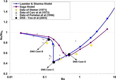
Figure 1. Normalized Nusselt number distribution in ascending mixed convection flows.

“Laminarization” (or “re-laminarization”) is an important topic in heat transfer and turbulence modeling [1] and is relevant to a wide range of applications. The test case considered in the present study is related to the post-trip decay heat removal in nuclear reactor cores. The primary focus of this paper is on ascending mixed convection flows representing coolant flow in the fuel elements of the UK fleet of Advanced Gas-cooled Reactors (AGRs) [2]. The review papers of Jackson et al. [3] and Jackson [4] provide extended discussions of heat transfer performance under mixed convection conditions. The most popular computational fluid dynamics (CFD) technique adopted in simulating mixed convection flows is based on the solution of Reynolds-averaged Navier–Stokes (RANS) equations, and among the possible turbulence models available to close these equations, eddy-viscosity models (EVMs) have been employed by the majority of researchers including Abdelmeguid and Spalding [5], Tanaka et al. [6], Cotton and Jackson [7], Mikielewicz et al. [8], Richards et al. [9], Kim et al. [10], and Keshmiri et al. [111213], among others. Keshmiri et al. [11, 12] recently tested a wide range of RANS turbulence models and found that the k-ω-SST model [14] and the nonlinear eddy-viscosity model (NLEVM) of Craft, Launder, and Suga [15] completely failed to capture the laminarization phenomenon present in ascending mixed convection flows. This was a particularly significant finding, since these two models are commonly used in several commercial CFD codes and are “recommended” by various industrial best practice guidelines for a wide range of applications [13, 16]. Indeed, contrary to expectation associated with some of the more recent turbulence models tested, it was demonstrated that the original “low-Reynolds number” model of Launder and Sharma [17] was, in general, the superior model.

The present research focusses on the NLEVM proposed by Craft, Launder, and Suga [15] and aims to investigate the reasons for the failure of this model in a benchmark ascending mixed convection flow. While the test case is indeed simple, it provides an unambiguous assessment of the physics associated with re-laminarization, and thus observations can be expected to be relevant to more complex applications. While some attempts are made to remedy the identified problem, the calibration of an entirely new model is beyond the scope of this study. Herein we aim to provide information for the purpose of a future study in this direction – i.e., the development of a cubic NLEVM for mixed convection flow, which would be of significant benefit to the nuclear industry.

2. Case description

The geometry studied here consists of a vertical pipe for which the thermal boundary condition is one of uniform wall heat flux. The working fluid is assumed to be standard air and the Reynolds number based on the pipe diameter is set to Re = 5,300. The Prandtl number of standard air (Pr = 0.71) is used throughout calculations. In addition, all fluid properties are assumed to be constant, and buoyancy is accounted for within the Boussinesq approximation.

In the results reported in this paper, comparison is made with the direct numerical simulation (DNS) data of You et al. [18], who conducted a study of turbulent mixed convection in a vertical uniformly heated pipe for constant property conditions. In their work, You et al. accounted for buoyancy via the Boussinesq approximation, which is particularly useful for validation studies since it permits an examination of buoyancy effects in isolation from other variable property phenomena. In computing mixed convection flows, You et al. [18] retained the same Reynolds and Prandtl numbers and varied buoyancy influence via the Grashof number. A total of four simulations were reported, as shown in Table 1, and a brief description of the thermal-hydraulic regime is provided in each case. The mean flow and turbulence profiles presented in Section 6 are reported for the four thermal-hydraulic regimes indicated in Table 1. These flow regimes have been chosen by You et al. specifically to correspond to one forced and three distinctive mixed convection cases. From the turbulence modeling point of view, Case (C) represents the most challenging thermal-hydraulic regime and is therefore viewed as the most important case in the present study.

Table 1. DNS cases from You et al. [18].

Case	Gr/Re^2	Bo	Thermal-hydraulic regime
A	0	0	Forced convection
B	0.252	0.13	Early-onset mixed convection
C	0.348	0.18	Laminarization
D	0.964	0.50	Recovery

3. Computational code and mesh

The present computations were performed using an in-house code, known as CONVERT (Convection in Vertical Tubes). CONVERT was originally developed by Cotton [19] and later extended by a number of researchers; the latest version used here is from Keshmiri et al. [11]. Differential equations are integrated over a control volume and then discretized, following a parabolic time-marching approach similar to the code described in Leschziner [20]. Solution of the algebraic equations is achieved via the Tri-Diagonal Matrix Algorithm (TDMA).

The mesh used for the present CONVERT computations consists of 100 control volumes and the wall-adjacent node is typically located at y⁺ = 0.5, never higher than unity. A number of tests with varying mesh refinement were carried out to ensure grid independence prior to obtaining the results reported below. In all cases, the solution is initialized with an isothermal run in which the dynamic field is allowed to develop from approximate initial profiles to a fully developed state. The production runs read the initialized results at the “location” x = 0 and are typically run for a time corresponding to a flow of 50 diameters downstream of x = 0. Interested readers are referred to Cotton [19] and Keshmiri et al. [11] for further details on the CONVERT solution sequence.

4. Mean flow equations

The mean flow equations are written in the Boussinesq approximation. Adopting Cartesian tensor notation, the equations read as follows:

Continuity:

(1)

Momentum:

(2)

Energy:

(3)

where g_i = [−g, 0, 0] in ascending flow, represents the Reynolds stress tensor, and the turbulent heat flux. In the present computations the turbulent heat fluxes are modeled using the simple eddy-diffusivity approximation, modeled as

(4)

Following standard modeling practice, the turbulent Prandtl number is set to a constant value, σ_t = 0.9.

5. The turbulence models

As mentioned above, computations in the present work are conducted using two low-Reynolds number eddy-viscosity-based models, namely the baseline k-ε model from Launder–Sharma (LS) [17] and the nonlinear k–ε model proposed by Craft, Launder, and Suga [15]. Nonlinear EVMs are, perhaps unsurprisingly, intended to offer a greater level of physical realism than the linear k-ε model, particularly for the complex geometries one is likely to be faced with in industry [1]. While reported in its full form by Craft et al. [15], this model was originally developed by Suga [21] and is thus here referred to as the “Suga” model. This model was popularized via its implementation in various commercial CFD software applications and should improve prediction of turbulence stress anisotropy via the incorporation of additional terms in the constitutive equation, both quadratic and cubic, in mean strain and vorticity. This is particularly significant close to a wall where stress anisotropy is high. Both models were implemented into CONVERT and validated with results from Suga [21] for a channel flow at Re = 5,600 and 14,000 (based on the DNS data of Kim et al. [22]). The results of these verification and validation tests can be found in [13, 23].

For clarity, the full form of both the LS and the Suga models is reviewed in this section. Both employ the same transport equations for turbulence kinetic energy and dissipation rate:

(5)

Given the focus of this paper, it is interesting to examine all points where these two models differ, and a full list of such is provided in Table 2. The model constants are the same for each model where the same constants exist (see Tables 3 and 4).

Table 2. Functions appearing in the LS and Suga turbulence models.

Variable	LS k-ε model	Suga k-ε model
	− νtSij + (2/3)kδij
Cμ	0.09
fμ		1 − exp[ − (Ret/90)^1/2 − (Ret/400)^2]
Eε

Table 3. Constants appearing in the LS and Suga models.

Constant	LS k-ε model	Suga k-ε model
σk	1.0	1.0
σε	1.3	1.3
Cϵ1	1.44	1.44
Cϵ2	1.92	1.92

Table 4. Constants appearing in the Reynolds shear stress equation of the Suga model.

c1	c2	c3	c4	c5	c6	c7
−0.1	0.1	0.26	−10 Cμ^2	0	−5 Cμ^2	5 Cμ^2

Note that both models solve for the homogenous dissipation rate, , rather than ϵ. This removes the need for an imposed finite value for the turbulence dissipation rate at the wall and thus increases stability of the model. The substitution is straightforward, since outside the viscous sub-layer , which means all the earlier modeling considerations are still valid, at the wall  = 0. Also shown in Table 2, the Suga model employs a “strain-sensitive” C_μ coefficient rather than the constant value C_μ = 0.09 used in the LS model. The proposed expression for C_μ is a function of dimensionless strain and vorticity invariants, which are defined as

(6)

where the mean strain rate and vorticity tensor are

(7)

Although this variable form of C_μ is expected to improve the prediction of turbulence in response to non-equilibrium strain rates, it does not imply any normal stress anisotropy. Instead, additional terms are added to the stress–strain relation which approximate the Reynolds stresses via a function of mean velocities and vorticities. Craft et al. [15] optimized the coefficients appearing in the constitutive equation of the Suga model over a range of flows including simple shear, impinging, curved and swirling flows. Their proposed values are listed in Table 4. Another term sometimes included in the ε-equation of the LS and Suga models is the Yap term (proposed by Yap [24]), which is a length-scale correction term. This correction was designed to prevent the LS model from returning excessively large length-scales, especially in reattaching and impinging flows; however, it has not been included in the calculations presented in the present paper since Keshmiri [12] has shown that, in ascending mixed convection flows, including the Yap term has no effects on heat transfer and friction coefficient. Generally, this correction term becomes active when the predicted turbulent length-scale exceeds the equilibrium length-scale, which is not the case in ascending mixed convection flow problems.

Finally, from Table 2 it can be seen that the expression for near-wall source term, E_ε, is different from its original form in the LS model. This term acts to increase the dissipation rate in the near-wall region, where velocity gradients change rapidly. A new expression for E_ε has been adopted in the Suga model in order to reduce its dependence on Reynolds number.

6. Results and discussion

6.1. Results of forced convection

Since forced convection Nusselt number (Nu₀) and friction coefficient (c_f0) provide the normalizing parameter in the presentation of heat transfer and friction coefficient impairment/enhancement effects, it is appropriate first to assess model performance in the computation of buoyancy-free pipe flows. The results of this initial assessment are summarized in Table 5, which compares the values of local Nusselt number and friction coefficient obtained by the Suga and LS models against the DNS data of You et al. [18]. It is noted that the LS model somewhat underpredicts the DNS values of Nu₀ and c_f0, while the value of Nu₀ returned by the Suga model is in very good agreement with the DNS data. The prediction of the Suga model for the friction coefficient is also closer to the data compared with the LS model.

Table 5. Results for fully developed forced convection.

Model/Technique	Nu0	% diff.	cf0	% diff.
DNS of You et al. [18]	18.3	–	9.28 × 10^−3	–
Launder–Sharma model	17.4	−4.9	8.52 × 10^−3	−8.2
Suga model	18.3	0	8.93 × 10^−3	−3.8

6.2. Results of local Nusselt number and friction coefficient

Figure 1 shows the heat transfer performance for both the Suga and LS models for an ascending flow. The Nusselt number in mixed convection, Nu, is normalized by the corresponding forced convection value evaluated at the same Reynolds and Prandtl numbers, and Nu/Nu₀ is plotted against the buoyancy parameter, Bo. The DNS data of You et al. [18], and the experimental results of Steiner [25], Carr et al. [26], and Parlatan et al. [27] are also included. The most remarkable observation from Figure 1 is the dramatic reduction in heat transfer levels occurring in the interval 0.15 < Bo < 0.25. Recall that DNS Case (C) (Bo = 0.18) is representative of the laminarized state, in which heat transfer levels are around 40% of those found in forced convection, under otherwise identical conditions. It can be seen that the predictions of the LS model formulation are in close agreement with the three DNS data points. The shortcoming of the Suga model is then immediately clear, in that the model appears to be unable to predict the correct level of heat transfer impairment indicated by DNS. Furthermore, the onset of this impairment is delayed significantly. However, in the “recovery” region (Bo ≥ 0.5) the Suga model is in reasonable agreement with the data of Steiner [25].

Turning to examine the friction coefficient, Figure 2 displays the normalized local friction coefficient plotted against the buoyancy parameter. Both models indicate little or no reduction in friction coefficient below the c_f0 level. In the case of the LS model this is, at least in part, related to its underprediction of c_f0 by about 8% (Table 5). In turn, this results in an earlier onset of friction coefficient enhancement compared with the experimental results of Carr et al. [26] and DNS data. In comparison with the LS model, the results of the Suga model indicate a steeper enhancement gradient.

Figure 2. Normalized friction coefficient distribution in ascending mixed convection flows.

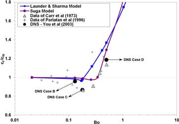
In comparing Figures 1–2, it is noted that the reduction of friction coefficient due to laminarization is significantly less than that of heat transfer. In addition, c_f/c_f0 rises to a value greater than unity for Case (C) (Bo = 0.18), while under the same conditions the heat transfer coefficient is much lower than 1. These differences lead to the conclusion that in a buoyancy-influenced flow the relationship between momentum transfer and heat transfer is less direct than in forced convection [10].

It is worth noting that in both Figures 1 and 2 there is some scatter in the reference data, particularly the experimental measurements of Parlatan et al. [27]. In their DNS work, You et al. [18] explained that while their results did not agree well with experimental data obtained by imposing the total pressure drop (e.g., Parlatan et al. [27]), they observed closer agreement with those obtained by measurement of velocity gradient instead (e.g., Carr et al. [26]). In addition, discrepancies are likely to arise from different methods of measuring c_f.

6.3. Mean flow profiles

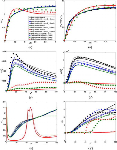
Mean flow and turbulent shear stress profiles obtained using both the Suga and LS models are plotted in Figure 3. Focussing first of all on the predictions from the Suga model, it can be seen from Figures 3a and 3b that the velocity predictions of the Suga model for the first three cases (Cases A–C) remain essentially unchanged, demonstrating the insensitivity of this model to the laminarization effect. The Suga model is then observed to respond correctly to buoyancy effects at higher Bo numbers, as indicated by the “M-shaped” profile for Case (D). In both velocity and temperature profiles, the maximum discrepancies occur at the pipe centerline, particularly so for Case (C). Considering now the same analysis for the LS model, a much improved response to the different conditions is observed. Results for Cases (A) and (B) are good, and while those for (C) and (D) exhibit a slight under-prediction of momentum at the centerline they are much improved versus the same predictions from the Suga model. It is worth also noting from Figure 3b that the mean velocity profiles are plotted in wall coordinates and highlight the departure from near-wall “universality” (i.e., the log-law) under conditions of turbulent mixed convection. As such, any assumption of universality made in order to construct wall functions for use with high-Reynolds number turbulence models applied to mixed convection is clearly questionable, underlining the need for modeling of the viscous sub-layer in these flows [7].

Figure 3. Mean flow profiles obtained using the Suga and Launder–Sharma models.

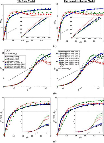
In Figure 3c, the temperature profiles returned by the LS model are in very good agreement with the DNS data, while the Suga model returns poor results for Cases (C) and (D). When plotting the temperature profiles in wall units (shown as insets in Figure 3c), these discrepancies become more apparent. This is particularly evident from the results of the Suga model, mainly due to an inaccurate estimation of τ_w by the model (see also friction coefficient distributions in Figure 2).

Already a general trend is emerging: that the extra modeling complexity afforded by the Suga model enables a slight but noticeable improvement in forced convection and early-onset mixed convection (i.e., Cases A and B). The same model is, however late in predicting re-laminarization and associated effects, and is thus in far poorer agreement with the reference results than its baseline model (LS).

6.4. Turbulence Quantities

Profiles of turbulent kinetic energy (TKE) and its dissipation rate, ε, are shown in Figures 4a and 4b, respectively. Once again, the predictions of the Suga model for forced convection and early-onset mixed convection (i.e., cases A and B) are significantly better than with LS. Indeed, the underprediction of peak TKE by the LS model is well known and has been reported by a number of other researchers including Patel et al. [28] and Cotton and Kirwin [29]. Nevertheless, the re-laminarizing effect of buoyancy on turbulence is at least qualitatively captured by the LS model (Case C), as is the recovery of k for Case (D). In contrast, the results of the Suga model for Cases (C) and (D) are severely over- and underpredicted, respectively.

Figure 4. Turbulence parameters of the Suga and LS models.

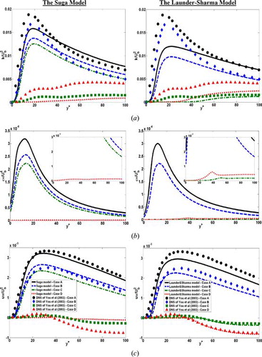
A similar trend can also be seen for the dissipation rate in Figure 4b. Although no profile was reported for ε by You et al., none of the profiles shown in Figure 4b are expected to be in good agreement with the DNS data especially near the wall, due to highly approximate nature of the ε-equation [30]. The differences between the predictions of LS and Suga models seen in Figure 4b are partly associated with different definitions of the “E-term” in the ε-transport equations of the models (compared in Table 2). This point will be discussed further in Section 6.6.4.

The Reynolds shear stress profiles are shown in Figure 4c. Cases (A) and (B) are seen to have similar shear stress profiles, in that they are positive and peak in the region y⁺ ≈ 20–30. In both cases (where forced convection is dominant), the predictions of the Suga model are in better agreement with the data than the LS model, as one might expect. For Case (C) it is observed that the DNS data indicate a laminarization of the flow, and a change in sign of the Reynolds stress in the core region. This reduction in stress levels is captured only by the LS model, which as discussed further on predicts almost complete laminarization of the near-wall flow. In contrast, the Suga model is completely insensitive to the laminarization effects at these conditions. The LS model captures the general trend of the data for Case (D), but fails to resolve the detail of near-wall stress distribution, while the Suga model significantly underpredicts the magnitude of shear stress, especially in the core region.

The turbulent viscosity ratio (TVR) is compared in Figure 5a, where the impact of the above differences becomes more relevant, especially for Cases (C) and (D). In the LS model, the magnitude of the reduction in TVR in comparison with Cases (B) to (C) is predicted correctly, i.e., the magnitude of the turbulent viscosity reduces by increasing the buoyancy influence, until complete laminarization occurs (Case C). With further increase in the effects of buoyancy, the region of zero TVR reduces which indicates that some turbulence recovery is occurring (Case D). Comparing the two sets of profiles in Figure 5a suggests that the failure of the Suga model may be linked to the way that turbulent viscosity is permitted to respond to the increase in buoyancy influence. The reduction of TVR with respect to buoyancy influence is severely underpredicted by the Suga model. This underprediction is consistent with the underprediction of heat transfer impairment observed in Figure 1.

Figure 5. Turbulent viscosity ratio and damping function from the Suga and LS models.

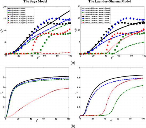
Profiles of the damping function, f_μ, are given in Figure 5b. Although the definition of f_μ in the Suga model is slightly different from that used in the LS model (compared in Table 2), the profiles for Cases (A) and (B) are somewhat similar. The profiles for Cases (C) and (D), however, are very different from those returned by the LS model, mainly due to differences in the distribution of Re_t which itself is proportional to k²/ϵ. It is worth noting that even in nonlinear EVMs such as the Suga model, a Reynolds number-dependent damping term (i.e., f_μ) is required for near-wall flows, but its influence is considerably less than that used in linear EVMs, since a substantial amount of the near-wall strain-related damping is now provided by the functional form of C_μ [15] (this point is discussed further in Sections 6.6.1 and 6.6.3).

6.5. Budgets of the TKE

While examining the TKE, or the rate of its dissipation is instructive, it is difficult to identify the source of a modeling problem by this process alone. Therefore, in order to see the influence of minor change of terms in a model, we here examine the individual contribution of each term required for a balance of the modeling equations set out above – i.e., the budget of the transport equations. The budgets of the TKE for forced convection and laminarization (i.e., Cases A and C) are plotted for both the Suga and LS models and are shown in Figure 6. Note that positive values indicate a local gain in TKE while negative values indicate a loss.

Figure 6. Budgets of turbulent kinetic energy obtained using the Suga and Launder–Sharma model; (a) Case A (forced convection) and (b) Case C (laminarization).

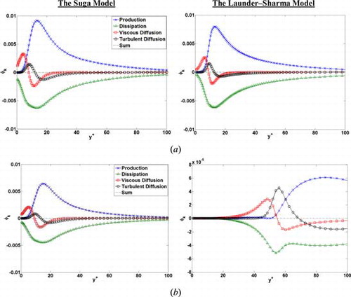
Figure 6a shows the balance of terms in the k-equation, calculated for fully developed forced convection (Case A) using the Suga and LS models. Similar trends are predicted by both models, even though the LS model indicates slightly lower values. It is seen that the budgets returned by both models are largely dominated by production and dissipation, except in the near-wall region. Very near to the wall, dissipation is balanced by viscous diffusion and the maximum production and dissipation of k occur at y⁺≈ 12. Also note that the viscous and turbulent diffusions change sign at approximately y⁺ ≈ 10 and y⁺≈ 13, respectively. The same is plotted for Case (C) in Figure 6b, where the LS model returns a dramatically different balance from that of forced convection. As expected, in the results of the LS model, it can be seen that the values are much lower than those of forced convection (by nearly two orders of magnitude), which are the indicators of laminarization. In this case all the elements of the k-budget are equal to zero up to y⁺ ≈ 20. The production of k remains zero at the position where maximum velocity occurs (i.e., y⁺ ≈ 40). Unlike Case (A), however, in the core region the production is balanced by the diffusion and dissipation terms. Contrary to this, the Suga model remains relatively insensitive to laminarization and thus is unable to predict the expected drop in turbulence.

6.6. Further modeling refinements

6.6.1. Numerical instability issues

During the course of the present study, significant numerical instability issues were encountered with the Suga model, particularly for higher heat loading values (i.e., higher values of Bo). In fact, similar problems were found when simulating the same test case using the commercial code, STAR-CD (reported in [11]). Another example of these numerical issues was reported by Yakinthos et al. [31] for the simulation of a 90° rectangular duct. An attempt to resolve these issues was made by the original authors and their colleagues, including the work by Cooper [32], Raisee [33], and Craft et al. [34]. The investigations of Raisee [33] on ribbed passages identified the dependence of C_μ on strain rate as the source of some of these problems. A subsequent investigation by Cooper [32] for an abrupt pipe expansion case indicated that the heat transfer overprediction of the Suga model was, at least in part, due to the fact that C_μ exceeded its equilibrium value in regions of low near-wall strain rate, and hence, limitation of the maximum value of C_μ was proposed, with some success. However, the numerical instability of the Suga model has not been investigated previously for mixed convection flows, where severe numerical issues have repeatedly been reported [111213].

In light of the above findings, and motivated to further investigate the instability issues of the Suga model, the distribution of C_μ and non-dimensional strain rate, , were examined, as plotted in Figure 7a and (b). Of most interest are the results associated with the recovery case, i.e., Case (D), which has been identified as the most numerically unstable. The C_μ profile for Case (D) exhibits a complex behavior, quite different to the other cases. Observed high levels of strain rate variation in the near-wall region (y⁺ < 5) in Figure 7b are associated with a sharp reduction in C_μ; this is a coupled effect, likely to be linked to the numerical instability in question. Further away from the wall, in the region of 40 < y⁺ < 60, C_μ rises suddenly, which corresponds to a region of low strain rate (corresponding to the maximum of the velocity profile in Figure 3b). In fact, at y⁺ ≈ 45, the model predicts zero strain rate, which in turn leads to a brief discontinuity in C_μ distribution. In regard to the majority of low-Reynolds number EVMs, a damping function appears in the expression of turbulent viscosity, and is usually denoted as f_μ. Similar to the LS model, the Suga model employs a Re_t-dependent damping function, albeit in a different form. Overall damping of turbulent viscosity can be achieved through f_μ × C_μ, which is plotted in Figure 7c. Comparing the distribution in Figure 7c to that in Figure 7a reveals the significant impact of C_μ on the overall damping of the Suga model.

Figure 7. Distribution of various low-Reynolds number functions in the Suga model.

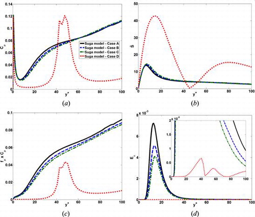
Finally, Figure 7d shows the distribution of E_εfor all four cases. For Cases (A)–(C), this source term is only significant within 5 < y⁺ < 50 and it peaks at y⁺ ≈ 15, which is consistent with the profiles of ε shown in Figure 4c. The profile of E_ε for Case (D), however, exhibits a very different trend, which includes a number of minima and maxima (shown more clearly in the inset) due to marked strain rate gradients and inaccurate turbulent viscosity predictions within 40 < y⁺ < 60.

6.6.2. Constant C_μ

Based on the observations discussed above, the first step to determine the source of numerical instability in the present simulations would be to investigate the effects of changing the C_μ formulation in the Suga model. In order to do so, in common with the majority of the two-equation EVMs, a constant value of C_μ = 0.09 was used in this part of the study to replace the “strain-sensitive” C_μ formulation in the original Suga model (see Table 2).

The calculations are repeated for all four thermal-hydraulic cases and initially it was found that setting C_μ to a constant value significantly improved the convergence and numerical instability of the Suga model. However, from the mean flow and temperature profiles shown in Figures 8a and 8b, it is evident that the Suga model with a constant C_μ, completely loses its sensitivity to laminarization effects and returns profiles that are entirely turbulent for all four thermal-hydraulic regimes. The inaccuracy of the modified Suga model is further evident from the severe overprediction of TKE and Reynolds shear stress in Figures 8c and 8d, compared with the DNS data and even the original Suga model. The failure of the modified Suga model seen in Figure 8 is mainly due to insufficient overall damping of the turbulent viscosity (represented by f_μ × C_μ) in the near-wall region, as seen in Figure 8e.

Figure 8. Effects of setting C_μ = 0.09 in the Suga model.

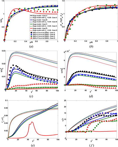
As alluded to earlier, in the original Suga model a substantial amount of near-wall strain-related damping is provided by the strain-sensitive C_μ function. Therefore, adopting a constant value for C_μ would produce insufficient damping of turbulent viscosity in the near-wall region. Therefore, the modified Suga model returns high levels of TVR in all four cases (Figure 8f), which is ultimately responsible for returning poor mean flow and temperature profiles (Figures 8a and 8b).

6.6.3. New C_μ formulation

As discussed in the previous sections, it is evident that the numerical instability issues of the Suga model in mixed convection flows are associated with the definition of C_μ. It was also found that using a constant value for C_μ has adverse effects on the performance of the model. Therefore, it is desirable to search for an alternative strain-sensitive definition for C_μ, which would ideally improve both the accuracy and stability of the Suga model.

Following the work of Craft et al. [34] for a sudden pipe expansion and an impinging jet, in this paper we propose the following alternative expression for C_μ:

(8)

where

(9)

(10)

This definition for C_μ, which has never previously been tested for mixed convection flows, is likely to reduce the sensitivity of C_μ to strain rate in those regions further away from the wall (and potentially removes the need for smoothing C_μ). In addition, it limits the maximum value of C_μ in regions of low strain rate, hence resolving the problem seen in Figure 7a, above.

The results of using the above definition for C_μ are shown in Figure 9. In Figures 9a and 9b it is evident that the mean flow and temperature profiles are only marginally affected by the new C_μ expression. However, the TKE and Reynolds shear stress profiles (Figures 9c and 9d) are affected to a greater extent: they are both indicated to be slightly higher as a consequence of a similar rise in levels of C_μ itself (Figure 9e). The new C_μ formulation also limits the maximum value of C_μ in regions of low strain rate: y⁺ > 65 for Cases (A)–(C) and 40 < y⁺ < 50 for Case (D). The low-strain rate region (i.e., approximately  < 5) in Case (D) corresponds to the peak region of the velocity profile.

Figure 9. Effects of using a new C_μ expression in the Suga model.

Furthermore, as can be seen in Figure 9f, for Cases (A)–(C) the new C_μ expression results in slightly higher levels of TVR in the near-wall regions. However, due to a “limiter” in Eq. (8), the new C_μ expression returns lower µ_t/µ in the core region (y⁺ > 80), a behavior somewhat similar to that of the LS model (see Figure 5a).

It is important to highlight that, while no significant improvement was achieved by using the new C_μ expression, the numerical stability of the Suga model improved remarkably. With the original Suga model, the present flow domain would not run beyond a distance of 50D (see Section 3), despite many attempts to fine-tune the numerics. However, with the new C_μ expression, convergence was obtained for a flow domain extended up to 500D. This finding confirms that the dependence of C_μ on strain rate is undoubtedly the main source of numerical instability in the original Suga model. This finding provides a new opportunity for the turbulence modeling community to test alternative strain-sensitive C_μ formulations, similar to the testing in the present work, with the aim of improving the accuracy and stability of this popular NLEVM.

6.6.4. The effects of E-term

In the present work, each of the four differences between the two models (summarized in Table 2) was tested systematically in order to isolate the root cause of the modeling failure in the laminarization case (i.e., Case C). The outcome of this trial suggested that the E-term (E_ε) in the original Suga model might be a source of inaccuracy in capturing laminarization effects. While the LS model uses a similar near-wall source term, the expression of E_ε in the original Suga model was designed to be less dependent on Reynolds number. To further investigate this point, the E-term in the original Suga model was replaced with that of the LS model and the simulations were repeated for all four thermal-hydraulic regimes given in Table 1, and the results are compared in Figure 10.

Figure 10. Effects of replacing the E-term of the original Suga model with that of the LS model.

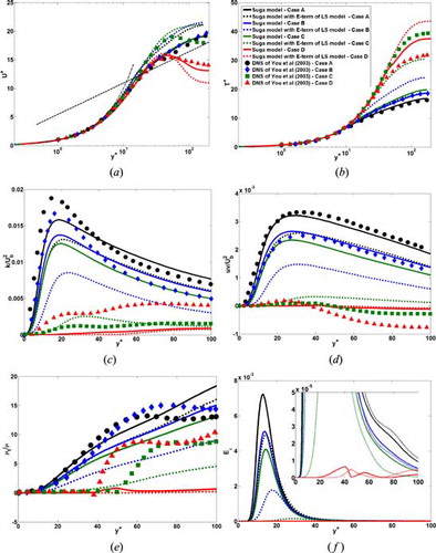
The mean flow and temperature profiles shown in Figure 10a and 10b indicate that the modified Suga model returns higher velocity magnitude for Cases (A)–(C) and higher temperatures in all cases, in the core region. It can also be seen that compared with the original model, the modified Suga model is generally in poorer agreement with the DNS data in all four cases. However, it is important to highlight that the E-term substitution reintroduced sensitivity among Cases (A)–(C) when compared to the original form of the Suga model. This sensitivity has more pronounced effects on the TKE and Reynolds shear stress profiles shown in Figure 10c and 10d, where the differences among thermal-hydraulic cases are more significant compared with the original model. This suggests that changing the E-term would enable the Suga model to become more sensitive to heat loading (i.e., the type of thermal-hydraulic regime), which for example results in better predictions for Case (C) in Figures 10c and 10d.

Figure 10e compares the distribution of E_ε for both the modified and original Suga models. Consistent with the TKE profiles, the modified Suga model returns significantly lower values, with the highest and lowest differences found for Cases (C) and (D), respectively.

The marked underprediction of TKE in Figure 10c resulted in the modified Suga model returning a lower value of µ_t/µ in Figure 10f for both near-wall and core regions compared with the original Suga model, in spite of both models having a similar profile. It is also noted that the largest discrepancy between the two models can be found in Case (C). Furthermore, in Figure 10f it can be seen that for Cases (A)–(C), the TVR in both the original and modified Suga models tends to increase almost linearly with respect to distance from the wall. This is mainly due to a quasi-linear overall damping of the turbulent viscosity in both models, represented by f_μ × C_μ(see Figure 7c), which is not directly influenced by the E-term definition. In contrast, the DNS data (and to a lesser extent the LS model – Figure 5a) show a small increase in TVR beyond y⁺ > 60 in all four cases. The discrepancy between the Suga model and the DNS data in predicting turbulent viscosity, especially in the core region, indicates the potential of using alternative damping functions, which tend to limit turbulent viscosity in the core region.

The results presented in this section generally indicate that replacing the E-term of the original Suga model with that of the LS model results in better prediction for the laminarization case (Case C), especially in predicting the level of TKE. However, the performance for Cases (A) and (B) is noticeably inferior and, therefore, further work is required in order to refine and calibrate this term to isolate this improvement to re-laminarization flow. This aspect is beyond the scope of the present study and is left for future work.

7. Conclusion

This paper investigates the mean flow and heat transfer in an ascending turbulent mixed convection pipe flow, which represents the coolant flow in the fuel elements of the UK fleet of Advanced Gas-cooled Reactors (AGRs). The aim of the present work was to carry out a meticulous assessment of the Suga NLEVM to identify the reasons for the failure of this commonly used turbulence model in mixed convection flows. The findings of this work would, inter alia, provide input to the turbulence modeling community for improving the performance and stability of this model for future applications, especially in the nuclear industry. As part of this study, the Suga model was implemented in an in-house CFD code, CONVERT, which, after successful verification and validation tests, was used to conduct all the computations presented here. Mean flow, heat transfer, and turbulence parameters were obtained for four different thermal-hydraulic regimes (Table 1) and were compared against the predictions of the LS model and the DNS data.

The present study showed that indirect influence of buoyancy force on turbulence in an ascending vertical pipe flow is the dominant mechanism, resulting in laminarization and impairment of heat transfer. It was also shown that for the laminarization and recovery regimes, inaccurate prediction of k²/ϵ was responsible for returning inaccurate turbulent viscosity which in turn led to poor mean flow and heat transfer results.

Furthermore, the instability problems of the Suga model were also investigated and were shown to be related to the dependence of C_μ on strain rate, which also contributed to the poor performance of this model in predicting laminarization. Subsequently, we tested an alternative expression of C_μ proposed by Craft et al. [34], and this significantly improved the stability of the Suga model while the mean flow profiles were marginally affected.

In an attempt to improve the performance of the Suga model, additional numerical tests were carried out in which the E-term in the original Suga model was replaced with that of the LS model. It was shown that the modified Suga model became more sensitive to the thermal-hydraulic regime. In particular, this substitution brought a significant improvement in the case of flow re-laminarization. This work serves to demonstrate that the formulation of the E-term can play an important role in future tuning of the Suga model, especially in heat transfer problems.

Acknowledgments

The authors are pleased to acknowledge the contribution of their colleagues in the School of Mechanical, Aerospace and Civil Engineering (MACE) at the University of Manchester, especially Dr. M.A. Cotton and Professor D. Laurence.

References

- W. P. Jones and B. E. Launder, The Prediction of Laminarization with a Two-equation Model of Turbulence, Int. J. Heat Mass Transfer, vol. 15, pp. 301–314, 1972.
- A. Keshmiri, Three-dimensional Simulation of a Simplified Advanced Gas-cooled Reactor Fuel Elements, Nuclear Eng. Des., vol. 241, pp. 4122–4135, 2011.
- J. D. Jackson, M. A. Cotton, and B. P. Axcell, Studies of Mixed Convection in Vertical Tubes, Int. J. Heat Fluid Flow, vol. 10, pp. 2–15, 1989.
- J. D. Jackson, Studies of Buoyancy-influenced Turbulent Flow and Heat Transfer in Vertical Passages, Keynote Lecture, 13th Int. Heat Transfer Conf., ‘IHTC13’, Sydney, Australia, 2006.
- A. M. Abdelmeguid and D. B. Spalding, Turbulent Flow and Heat Transfer in Pipes with Buoyancy Effects, J. Fluid Mech., vol. 94, pp. 383–400, 1979.
- H. Tanaka, S. Maruyama, and S. Hatano, Combined Forced and Natural Convection Heat Transfer for Upward Flow in a Uniformly Heated Vertical Pipe, Int. J. Heat Mass Transfer, vol. 30, pp. 165–174, 1987.
- M. A. Cotton and J. D. Jackson, Vertical Tube Air Flows in the Turbulent Mixed Convection Regime Calculated using a Low-Reynolds-number k-ε Model, Int. J. Heat Mass Transfer, vol. 33, pp. 275–286, 1990.
- D. P. Mikielewicz, A. M. Shehata, J. D. Jackson, and D. M. McEligot, Temperature, Velocity and Mean Turbulence Structure in Strongly Heated Internal Gas Flows Comparison of Numerical Predictions with Data, Int. J. Heat Mass Transfer, vol. 45, pp. 4333–4352, 2002.
- A. H. Richards, R. E. Spall, and D. M. McEligot, An Assessment of Turbulence Models for Strongly-heated Internal Gas Flows, Proc. 15th IASTED Int. Conf. on Modeling and Simulation, Marina Del Rey, California, USA, 2004.
- W. S. Kim, S. He, and J. D. Jackson, Assessment by Comparison with DNS Data of Turbulence Models used in Simulations of Mixed Convection, Int. J. Heat Mass Transfer, vol. 51, pp. 1293–1312, 2008.
- A. Keshmiri, M. Cotton, Y. Addad, and D. Laurence, Turbulence Models and Large Eddy Simulations Applied to Ascending Mixed Convection Flows, Flow, Turbul. Combust., vol. 89, no. 3, pp. 407–434, 2012.
- A. Keshmiri, Effects of Various Physical and Numerical Parameters on Heat Transfer in Vertical Passages at Relatively Low Heat Loading, ASME J. Heat Transfer, vol. 133, pp. 092502–1, 2011.
- A. Keshmiri, J. C. Uribe, and N. Shokri, Benchmarking of Three Different CFD Codes in Simulating Natural, Forced and Mixed Convection Flows, J. Numer. Heat Transfer; Part A: Appl., vol. 67, pp. 1324–1351, 2015.
- F. R. Menter, Two-Equation Eddy-Viscosity Turbulence Models for Engineering Applications, AIAA J., vol. 32, pp. 1598–1605, 1994.
- T. J. Craft, B. E. Launder, and K. Suga, Development and Application of a Cubic Eddy-viscosity Model of Turbulence, Int. J. Heat Fluid Flow, vol. 17, pp. 108–115, 1996.
- J. Mahaffy, B. Chung, F. Dubois, F. Ducros, E. Graffard, M. Heitsch, M. Henriksson, E. Komen, F. Moretti, and T. Morii, Best Practice Guidelines for the use of CFD in Nuclear Reactor Safety Applications, NEA/CSNI/R(2007)5, May 15, 2007.
- B. E. Launder and B. I. Sharma, Application of the Energy Dissipation Model of Turbulence to the Calculation of Flow Near a Spinning Disc, Lett. Heat Mass Transfer, vol. 1, pp. 131–138, 1974.
- J. You, J. Y. Yoo, and H. Choi, Direct Numerical Simulation of Heated Vertical Air Flows in Fully Developed Turbulent Mixed Convection, Int. J. Heat Mass Transfer, vol. 46, pp. 1613–1627, 2003.
- M. A. Cotton, Theoretical Studies of Mixed Convection in Vertical Tubes, Ph.D. thesis, Dept. of Engineering, University of Manchester, UK, 1987.
- M. A. Leschziner, An Introduction and Guide to the Computer Code PASSABLE, Ph.D. Thesis, Dept. of Mech. Engineering, UMIST (now University of Manchester), 1982.
- K. Suga, Development, and Application of a Non-Linear Eddy Viscosity Model Sensitized to Stress, and Strain Invariants, Ph. D. Thesis, Dept. of Mechanical Engineering, UMIST (now University of Manchester), UK, 1995.
- J. Kim, P. Moin, and R. Moser, Turbulence Statistics in Fully Developed Channel Flow at Low Reynolds Number, J. Fluid Mech. Digital Arch., vol. 177, pp. 133–166, 1987.
- A. Keshmiri, Thermal-hydraulic Analysis of Gas-cooled Reactor Core Flows, Ph.D. thesis, School of Mechanical, Aerospace and Civil Engineering, University of Manchester, UK, 2010.
- C. R. Yap, Turbulent Heat, and Momentum Transfer in Recirculating, and Impinging Flows, Ph. D. Thesis, Dept. of Mech. Engineering, Faculty of Technology, UMIST (now University of Manchester), UK, 1987.
- A. Steiner, On the Reverse Transition of a Turbulent Flow under the Action of Buoyancy Forces, J. Fluid Mech., vol. 47, pp. 503–512, 1971.
- A. D. Carr, M. A. Connor, and H. O. Buhr. Velocity, Temperature, and Turbulence Measurements in Air for Pipe Flow with Combined Free, and Forced Convection, J. Heat Transfer, vol. 95, pp. 445–452, 1973. Trans. ASME C.
- Y. Parlatan, N. E. Todreas, and M. J. Driscoll, Buoyancy and Property Variation Effects in Turbulent Mixed Convection of Water in Vertical Tubes, J. Heat Transfer, vol. 118, pp. 381–387, 1996.
- V. C. Patel, W. Rodi, and G. Scheuerer, Turbulence Models for Near-wall and Low Reynolds Number Flows: A Review, AIAA J., vol. 23, pp. 1308–1319, 1985.
- M. A. Cotton and P. J. Kirwin, A Variant of the Low-Reynolds-number Two-equation Turbulence Model Applied to Variable Property Mixed Convection Flows, Int. J. Heat Fluid Flow, vol. 16, pp. 486–492, 1995.
- M. A. Cotton and J. O. Ismael, A Strain Parameter Turbulence Model and Its Application to Homogeneous and Thin Shear Flows, Int. J. Heat Fluid Flow, vol. 19, pp. 326–337, 1998.
- K. Yakinthos, Z. Vlahostergios, and A. Goulas, Modeling the Flow in a 90° Rectangular Duct using One Reynolds-stress and Two Eddy-viscosity Models, Int. J. Heat Fluid Flow, vol. 29, no. 1, pp. 35–47, 2008.
- D. Cooper Computation of Momentum, and Heat Transfer in a Separated Flow, using Low-Reynolds-number Linear, and Non-linear k-ϵ Models, M. Res. Dissertation, Dept. of Mechanical Engineering, UMIST (now University of Manchester), UK, 1997.
- M. Raisee Computation of Flow, and Heat Transfer through Two-, and Three-dimensional Rib-roughened Passages, Ph. D. Thesis, Dept. of Mechanical Engineering, UMIST (now University of Manchester), UK, 1999.
- T. J. Craft, H. Iacovides, and J. H. Yoon Progress in the use of Non-Linear Two-Equation Models in the Computation of Convective Heat Transfer in Impinging and Separated Flows, Flow, Turbul. Combust., vol. 63, pp. 59–80, 1999.