Heat transfer and pressure drop correlations for laminar flow in an in-line and staggered array of circular cylinders

Abstract

Enhanced heat transfer surfaces based on cylindrically shaped pin fins with wire diameters in the range of 100 µm were analyzed. The design is based on a high pin length to diameter ratio in the range of 20–100. Correlations for thermal and fluid dynamic characteristics of these fine wire structures are not available in literature. An in-line and staggered arrangement of pins were simulated for a variety of operational and geometrical conditions with a two-dimensional computational thermal and fluid dynamics model. Correlations for Nusselt number and friction factor with respect to Reynolds number and geometry were derived thereby. Reynolds numbers based on the wire diameter are in the range of 3–60. The correlations for the Nusselt number and friction factor can predict 93% and 97% of the simulated data within ±10%.

1. Introduction

In recent years, the development of cellular metal structures as heat transfer surface area enhancements has been intensified [1–3]. These structures are attractive for a wide range of applications where dissipation of heat over relatively small spaces is demanded. Engine cooling in the transport sector or heating, cooling, and air conditioning systems in buildings are two example applications. The cellular metal structures can be classified into two broad classes: one with a stochastic topology and the other with a periodic structure [4]. Examples of a stochastic topology include metal foams and packed beds. However, these structures generally have very high pressure drops due to their undirected microgeometry [2,5,6]. Likewise, the heat flux through undirected microgeometry is inhibited. Examples of periodic cellular metal structures include materials made from stacked or corrugated metal textiles, micro-pin fins [7], and microtruss concepts (e.g. tetrahedral, pyramidal, or Kagome topologies) [4,8].

The focus of this simulation study is on plate-fin wire structures with cylindrical shaped, parallel wires, as one subcategory of periodic cellular metal structures. In Figure 1, a plate-fin wire structure is shown as part of a flat tube heat exchanger. These plate-fin wire structures allow heat flux to be oriented normal to the primary surface separating the fluid from the heat source or sink (tubes, plates). Parallel wire structures can, on the one hand, be achieved by a pin fin structure, although its manufacturing is costly [9,10]. On the other hand, wire structures based on textile technology (e.g. weaving or knitting) can be oriented similarly, with the benefit of a highly developed manufacturing process. Currently, textile structures are used frequently as regenerators due to their high surface area density and less frequently for tube–fin heat exchangers [11].

Figure 1. Concept of a flat tube heat exchanger with plate-fin wire structure.

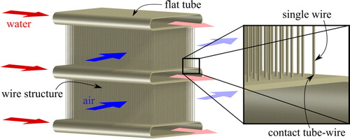
For the heat transfer enhancement in heat exchangers with low convective heat transport on the gas side, a variety of different wire structure design ideas are given in the literature and on the market. Those include metallic woven wire mesh structures [12–14] and screen-fin structures [15], which are contacted to a flat primary surface. One market available air-to-air heat exchanger with a separating plastic wall is manufactured by Vision4Energy [16]; performance evaluation is done by Bonestroo [17] numerically and by Fugmann et al. [18] numerically and experimentally. A section of this heat exchanger is shown in Figure 2a. Further numerical studies of pins with different cross-sectional shapes and a comparison of the thermal and fluid dynamic performances with louvered fins are given in Sahiti [19]. From this performance comparison, it was found that the pin fin heat exchanger is able to perform equally to a louvered fin heat exchanger, but with 22% less volume. The woven or knitted wire structures described in literature are predominantly limited to meshes, with additional wires only weakly supporting heat transfer. These impeding wires, yet creating pressure drop, are not directly contacted to the primary surface but oriented in parallel to the plates. Thus, heat transfer has to take place along multiple wires, with thermal contact resistance between each of them. Fugmann et al. [20] show the potential for a set of parallel wire structures without impeding wires based on computational fluid dynamics (CFD) simulations and measurements. Within two further studies [21,22], pin fin and woven wire structure samples have been manufactured and tested for thermal–hydraulic performance. Figures 2b and c show details of the structures with a wire length to diameter aspect ratio in the range of 40–100. For the wire structures, aluminum and copper are used, providing sufficiently high heat conductivity. The wire diameters range from 105 µm to 250 µm.

Figure 2. Different wire structure heat exchangers with high aspect ratio tested for thermal–hydraulic performance: (a) continuous wire structure; (b) pin fin structure; and (c) woven wire structure (adopted from [18,21,22]).

This simulation study extends the set of geometries and concentrates on the derivation of correlations for Nusselt number and friction factor. The simulation is necessary as available correlations on flow around cylinders do not cover the required range of geometry and operation parameters. Thus, this study supplements the existing literature correlations for heat transfer and pressure drop for the specific geometry and operating conditions used in fine wire structure heat exchangers. Thereby, it allows a performance estimation of geometries different than the specific geometries used in [18,21,22] and the possibility of optimizing the design for new sample manufacturing.

2. Model setup

2.1. Design idea

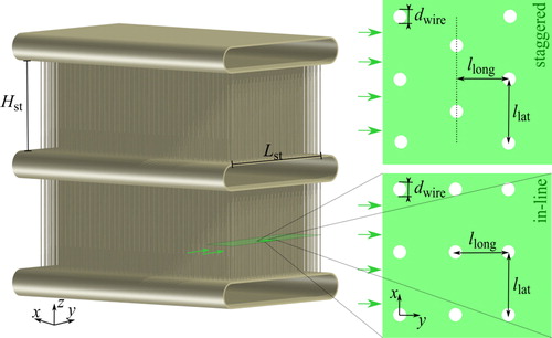
The design idea for a flat tube wire structure heat exchanger is related to a standard flat tube–fin design. The wires are arranged primarily perpendicular to the flat tubes (see Figure 1). The manufacturing can be based on corrugated textile fabrics or single wires cut to length. The bonding of wires to the tubes can be done by welding or soldering. In any case, the thermal resistance of contact can be a limiting factor. The arrangement of wires is dependent on the manufacturing process and it is either in-line, staggered, or differently patterned (see Figure 3). A different arrangement changes the thermal–hydraulic behavior of the heat exchanger and allows an adaption to a specific application. This study concentrates on air to water heat exchangers. However, due to the use of nondimensional numbers, the results can be transferred to other combinations. The heat transfer process can in short be described as follows (see Figure 1): hot water is passing the flat tubes. Heat is transferred by forced convection to the inner tube wall. Through the wall and the wires, heat conduction takes place. On the outer tube wall (primary surface) and the wires (secondary surface), heat is transferred by forced convection to the passing cold air.

Figure 3. Cross-section through a wire structure heat exchanger.

The heat transfer coefficient between the wires and the air increases with decreasing wire diameter. This is due to a reduction of the thermal boundary layer thickness and, therefore, larger temperature gradients in the gas flow (if the velocity is kept constant). This yields a heat transfer coefficient of approximately 500 W/m²K for the air flow around a single wire of 0.1 mm in diameter, at an inlet air temperature of 25 °C and a velocity of 2 m/s [23, Chapter Gf]. In addition, the material utilization for manufacturing wires is better than that for metal sheets with the same heat transfer surface area [20]. Assuming that the diameter of a wire is the same as the thickness of a metal sheet, the mass-specific surface area is twice that for the metal sheet. These positive effects have to outweigh possible drawbacks, which are related to high pressure drop through very dense cellular metal structures and low volume-specific heat transfer surfaces for very open cellular metal structures.

2.2. Model

Steady-state fluid flow and heat transfer was simulated using the finite element method (FEM), implemented in COMSOL Multiphysics^® (version 5.3). The continuity equation, Navier–Stokes equation, and energy (heat) equation describes the system on the air side:(1) $$\nabla ·\left({\rho }_{\text{air}}\mathrm{ }\mathbf{u}\right)=0$$(1) (2) $${\rho }_{\text{air}}\left(\mathbf{u}·\nabla \right)\mathbf{u}=\mathrm{ }\nabla ·[\mathrm{ }-p\mathbf{I}+{\mu }_{\text{air}}\left(\nabla \mathbf{u}+{\left(\nabla \mathbf{u}\right)}^{\mathrm{T}}\right)]$$(2) (3) $${\rho }_{\text{air}}{c}_{p,\text{air}}\mathbf{u}\cdot \nabla T=\mathrm{ }\nabla \cdot (k_{\text{air}}\nabla T)$$(3)

The material properties$\mathrm{ }{\rho }_{\text{air}}$,${\mathrm{ }\mu }_{\text{air}}$,${\mathrm{ }c}_{p,\text{air}}$, and $k_{\text{air}}$ are the density, dynamic viscosity, heat capacity at constant pressure, and thermal conductivity of air. Their values were fixed at 20 °C and 1 atm. The vector $\mathbf{I}$ is the identity. The scalars for temperature $T$, pressure $p$, and the velocity field $\mathbf{u}=(u,v)$ are the dependent variables. Several simplifications are related to the energy Eq. (3)(3) $${\rho }_{\text{air}}{c}_{p,\text{air}}\mathbf{u}\cdot \nabla T=\mathrm{ }\nabla \cdot (k_{\text{air}}\nabla T)$$(3) . First, the work related to a thermal expansion is neglected. Second, the influence of varying viscosity between the boundary layer and the bulk flow during heating or cooling is neglected [24, Ch. 3]. Both simplifications are motivated with a small impact on the performance as long as temperature differences within the fluid are moderate. Third, the viscous dissipation is neglected. Viscous dissipation could contribute significantly to heat generation, especially for fluids with small wall-to-fluid temperature differences [25, p. 53]. A possible evaluation criterion is given by the ratio of viscous heat generation to external heating, expressed with the Brinkman number ${\text{Br}}_{\text{air}}\mathrm{ }$[25, p. 54]:(4) $${\text{Br}}_{\text{air}}=\mathrm{ }\frac{{\mu }_{\text{air}}{v}_{\text{air}}^2}{k_{\text{air}}\left(T_{\text{wall}}-T_{\text{air},\mathrm{m}}\right)}$$(4)

Therein $v_{\text{air}}$ is a mean velocity through the structure and $\left(T_{\text{wall}}-T_{\text{air},\mathrm{m}}\right)$ is a mean temperature difference between the heated (or cooled) wall temperature $T_{\text{wall}}$ and the mean air temperature $T_{\text{air},\mathrm{m}}$. The Brinkman number is small ($\left|{\mathrm{B}\mathrm{r}}_{\text{air}}\right|<{10}^{-3}$) for applications with moderate velocities $v_{\text{air}}$ below 10 m/s and temperature differences $\left|T_{\text{wall}}-T_{\text{air},\mathrm{m}}\right|$ above 2 K (for air temperatures from 0 °C to 100 °C and atmospheric pressure 1 atm). For a wide variety of applications, this holds true, such that the scope of this study is on these applications.

A cross-section through a wire structure heat exchanger in the direction of air fluid flow is shown in Figure 3. In the cross-section, the wires appear as circular obstacles. Simulating flow and heat transfer around the wires in the two-dimensional (2D) cross-section can give a first estimate on the thermal–hydraulic behavior of the heat exchanger. The following assumptions AS1 to AS5 are taken for the heat exchanger geometry and the operating condition:

AS1: Gradients in z-direction of velocity, pressure, and temperature fields are negligibly small

AS2: Air velocity z-component is negligibly small (e.g., caused by reduction of free flow area due to blocking tubes)

AS3: Pressure drop associated with sudden contraction and expansion at the core structure inlet and outlet (due to the blocking tubes) is negligibly small or is known

AS4: Heat flux through the tube wall in direct contact to air is negligibly small or is known

AS5: Operation is steady state with uniform temperature and velocity profiles at the heat exchanger inlet

In this study, the wires are arranged symmetrically in x-direction, meaning that one characteristic in-line or staggered element represents the whole geometry. The characteristic element and the boundary conditions for temperature, pressure, and velocity for the steady-state laminar flow are shown for the in-line and staggered 2D cross-section in Figure 4. The symmetry conditions ensure that the influence of neighboring wires in x-direction on the flow is considered. Assumptions AS1 and AS2 are only valid if the height of the structure $H_{\text{st}}$ is at least 5 times higher than the lateral wire distance $l_{\text{lat}}$ (see geometry in Figure 3). Based on several three-dimensional (3D) simulations [26], the influence on the pressure drop and heat transfer coefficient was within ±5% above the ratio threshold of $H_{\text{st}}/l_{\text{lat}}>5$. Assumption AS3 can in general be reduced to an estimation of the pressure losses associated with free expansion that follow sudden contraction and pressure losses associated with the irreversible free expansion and momentum rate changes following an abrupt expansion. The related contraction and exit loss coefficient can be determined based on the literature values [11, p. 385–389]. Assumption AS4 is particularly fulfilled if the (tube wall) primary surface area $A_{\text{HTS},\mathrm{p}}$ is small in comparison with the structure surface area $A_{\text{HTS},\mathrm{s}\mathrm{t}}$. In the case of the wire structure, it holds $A_{\text{HTS},\mathrm{p}}/A_{\text{HTS},\mathrm{s}\mathrm{t}}<20\mathrm{\%}$ if $H_{\text{st}}/l_{\text{lat}}>5$ and $l_{\text{long}}/d_{\text{wire}}<1.5$. Additionally, the heat flux through the wall in direct contact to air is reduced due to a larger thermal boundary layer near the wall in comparison with the wires, expressed by high convection heat transfer coefficients for the wires.

Figure 4. Boundary conditions of the in-line (a) and staggered (b) cross-section model [18].

The characteristic element is determined by the wire diameter$\mathrm{ }{d}_{\text{wire}}$, the lateral and longitudinal distance of the wires, $l_{\text{lat}}$ and $l_{\text{long}},\mathrm{ }$respectively, and the total length of the structure$\mathrm{ }{L}_{\text{st}}$ or the number of wires $n_{\text{wires}}$ (see Figure 3). The air velocity field is determined by the structure inlet velocity $v_{\text{air},\mathrm{i}\mathrm{n},\mathrm{s}\mathrm{t}}$ and the inlet temperature$\mathrm{ }{T}_{\text{air},\mathrm{i}\mathrm{n}}$. The nondimensional input parameters of the model are given in Table 1. The choice of parameter ranges is related to available manufacturing possibilities and typical applications of air side heat transfer enhancement [18,20–22].

Table 1. Definition of nondimensional input parameters to simulation model with minimal and maximal values in parametric study.

Symbol	Definition	Description	Min.	Max.
$a$	$\frac{l_{\text{lat}}}{d_{\text{wire}}}$	Nondimensional lateral distance of the wires	2	12
$b$	$\frac{l_{\text{long}}}{d_{\text{wire}}}$	Nondimensional longitudinal distance of the wires	1.3	8
${\text{Re}}_{\text{air},\mathrm{s}\mathrm{t}}$	$\frac{v_{\text{air},\mathrm{i}\mathrm{n},\mathrm{s}\mathrm{t}}{\mathrm{ }d}_{\text{wire}}\mathrm{ }{\rho }_{\text{air}}}{{\mu }_{\text{air}}\mathrm{ }}$	Reynolds number	3	60
$n_{\text{wires}}$	$\frac{L_{\text{st}}}{l_{\text{long}}}\mathrm{ }$	Number of wires in flow direction	2	200
${\text{Pr}}_{\text{air}}\mathrm{ }$	$\frac{v_{\text{air},\mathrm{i}\mathrm{n},\mathrm{s}\mathrm{t}}{c}_{p,\text{air }}{\rho }_{\text{air}}}{k_{\text{air}}}$	Prandtl number	0.71	0.71

Neighboring wires in y-direction (main flow direction) affect fluid flow and temperature fields around a wire. Thus, a simulation run with a specific number of wires did not allow a distinct definition of thermal–hydraulic characteristics of a geometry with fewer wires. The number of wires had to be changed in each simulation run.

The meshing of the domain was separated into a triangular mesh next to the wires and a quadrilateral mesh further on (see Figure 5). The triangular and quadrilateral meshes were refined in order to obtain a mesh-independent solution. The Richardson method [27] was used to determine the order of accuracy of the mesh refinement. The normalized grid spacing was defined as the surface area of a quadrilateral element normalized with the surface area of the quadrilateral element of the finest mesh. The quadrilateral element of the finest mesh was equal to 2.5 µm × 2.5 µm. The length of one quadrilateral mesh element ranged from 2.5 µm to 25 µm in a geometry of 100 µm wire diameter. A direct evaluation of the order of convergence $p_{\text{mesh}}\mathrm{ }$could be obtained from three solutions using a constant grid refinement ratio${\mathrm{ }r}_{\text{mesh}}$. The Grid Convergence Index (GCI) based on the procedure for estimation of uncertainty due to discretization [27] is shown in Table 2. Thus, uncertainty due to discretization is lower than 0.05% for grids with normalized grid spacing 1 or 4. In this study, a normalized grid spacing of 4 will be used from now on.

Figure 5. Meshing of 2D cross-section with different levels of grid refinement.

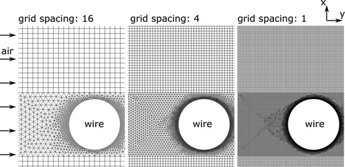
Table 2. Grid Convergence Index (GCI) based on Richardson method [27] for Nusselt number and friction factor.

Solution	$r_{\text{mesh}}$	$p_{\text{mesh}}$	${\text{GCI}}_{12}$ in %	${\text{GCI}}_{23}$ in %
Nusselt number	4	0.245	0.032	0.045
Friction factor	4	1.013	0.009	0.038

Geometry consists of five wires in row ($a$ = 8, $b$ = 3) at ${\text{Re}}_{\text{st}}$ = 11.25. Index 1 represents finer mesh, index 3 coarser mesh.

A similar GCI as in Table 2 could be achieved with number of wires equal to 30 and Reynolds numbers equal to 5.6, 11.2, and 22.5; all other parameters were kept constant. Grid Convergence Indices ${\text{GCI}}_{12}$ and ${\text{GCI}}_{23}$ were below 0.05%.

The CFD simulation was necessary as available data on flow around cylinders do not cover the required range of geometry and operation parameters for the present application. Within the VDI Wärmeatlas [23], correlations for Nusselt number based on Reynolds numbers below 100 and nondimensional wire distances below 4 can be found. However, according to the source of the correlation [28,29], the corresponding measurements were taken at Reynolds numbers above 1,000 for a Prandtl number in the required range of 1 (gas). Thus, the correlation does not include the present operation range.

A comparison of simulation to pressure drop measurement results of an in-line wire structure geometry ($a=4.2,\mathrm{ }b=6.7$) with $1<{\text{Re}}_{\text{air},\mathrm{s}\mathrm{t}}<25\mathrm{ }$based on [18] showed a good agreement of Fanning friction factor with a relative error between 2% and 20%. The simulation model was equal to the model used within this study. The same model was used in a further numerical and experimental comparison of thermal–hydraulic performance in [21]. The comparison showed a borderline agreement of Fanning friction factors for the staggered pin fin arrangement ($a=4.8,\mathrm{ }b=1.4$) with $10<{\text{Re}}_{\text{air},\mathrm{s}\mathrm{t}}<50$. Relative errors range from 10% to 40%. It showed an acceptable agreement of Nusselt numbers with a relative error between 2% and 25%. A main reason for the differences could be that the pin fin test core had geometrical irregularities due to the manual manufacturing process. As a result, some wires were not contacted or not homogeneously distributed. A reduction in thermal–hydraulic performance was plausible [21].

2.3. Data reduction parameters

The total heat flux in the simulated 2D heat exchanger $\dot{q}$(5) $$\dot{q}=v_{\text{air},\mathrm{i}\mathrm{n},\mathrm{s}\mathrm{t}}\mathrm{ }{\mathrm{l}}_{\text{lat}}\mathrm{ }{{\rho }_{\text{air}}\mathrm{ }c}_{p,\text{air}}\mathrm{ }\mathrm{\Delta }{T}_{\text{air}}$$(5) and the true (or effective) mean temperature difference also referred to as the mean temperature driving potential $\mathrm{\Delta }{T}_m$(6) $$\mathrm{\Delta }{T}_{\mathrm{m}}=\frac{{(T}_{\text{air},\text{in}}-T_{\text{wall}})\mathrm{ }-(T_{\text{air},\text{out}}-T_{\text{wall}})\mathrm{ }}{\ln \left(\frac{T_{\text{air},\text{in}}-T_{\text{wall}}}{T_{\text{air},\text{out}}-T_{\text{wall}}}\right)}$$(6) yield the convection heat transfer coefficient$\mathrm{ }{h}_{\text{air},\mathrm{s}\mathrm{t}}$(7) $$h_{\text{air},\mathrm{s}\mathrm{t}}=\frac{\dot{q}}{\Delta T_{\mathrm{m}}{A}_{\text{HTS}}^{\mathrm{\prime }}},$$(7) with $A_{\text{HTS}}^{\mathrm{\prime }}\mathrm{ }$being the sum of all wire perimeters.

The pressure drop $\mathrm{\Delta }{p}_{\text{air},\mathrm{s}\mathrm{t}}$ is calculated by taking the difference of the air inlet pressure and the air outlet pressure.

The Nusselt number on the air side is a nondimensional quantity, expressing the convective heat transfer versus the conductive heat transfer. It is defined as(8) $${\text{Nu}}_{\text{air},\mathrm{s}\mathrm{t}}=\frac{h_{\text{air},\mathrm{s}\mathrm{t}}{d}_{\text{wire}}}{k_{\text{air}}}.$$(8)

The nondimensional representation of pressure drop ${\mathrm{\Delta }p}_{\text{air},\mathrm{s}\mathrm{t}}$ can be realized by the Fanning friction factor $f_{\text{air},\mathrm{s}\mathrm{t}}$ which is given by(9) $$f_{\text{air},\mathrm{s}\mathrm{t}}=\frac{{\mathrm{\Delta }p}_{\text{air},\mathrm{s}\mathrm{t}}}{4\left(\frac{L_{\text{st}}}{d_{\text{wire}}}\right)\left(\frac{{\rho }_{\text{air }}{v}_{\text{air},\mathrm{i}\mathrm{n},\mathrm{s}\mathrm{t}}^2}{2\mathrm{ }}\right)}$$(9)

The nondimensional quantities can be related to the airside Reynolds number ${\text{Re}}_{\text{air},\mathrm{s}\mathrm{t}}$ and the Prandtl number$\mathrm{ }\mathrm{P}{\mathrm{r}}_{\text{air}}$.

3. Simulation results and derivation of correlation

3.1. Local and global definitions

The Nusselt number ${\text{Nu}}_{\text{st}}={\text{Nu}}_{\text{air},\mathrm{s}\mathrm{t}}$ was simulated and calculated for different number of wires. As the number of wires differed within different simulations, the number of wires is added to the Nusselt number as an index for reasons of clarity. The global Nusselt number ${\text{Nu}}_{\text{st}}$ is a mean of all wires within the domain. The local Nusselt number or thermal entrance Nusselt number $\mathrm{N}{\mathrm{u}}_{\mathrm{s}\mathrm{t},\text{local}}$ (cf. [11, p. 502]) for each wire is related to the global definition according to:(10) $$\mathrm{N}{\mathrm{u}}_{\mathrm{s}\mathrm{t},i}=\frac{1}{i-1}\underset{1}{\overset{i}{\int }}\mathrm{N}{\mathrm{u}}_{\mathrm{s}\mathrm{t},\text{local}}\left(y\right)dy$$(10) such that $\mathrm{N}{\mathrm{u}}_{\mathrm{s}\mathrm{t},1}=\mathrm{N}{\mathrm{u}}_{\mathrm{s}\mathrm{t},\text{local},1}$. When the number of wires increases, the global and local Nusselt number converges toward the same limit value. This limit value represents the Nusselt number in a thermally developed flow. The limit value is defined as(11) $$\mathrm{N}{\mathrm{u}}_{\mathrm{s}\mathrm{t},\mathrm{\infty }}\mathrm{ }=\mathrm{ }\mathrm{N}{\mathrm{u}}_{\mathrm{s}\mathrm{t},\text{local},\mathrm{\infty }}$$(11)

The flow direction through the heat exchanger is nondimensionalized as(12) $$y^{\mathrm{*}}=\frac{y}{d_{\text{wire}}b}$$(12) with $y\mathrm{ }=\mathrm{ }0$ representing the entrance of the heat exchanger structure. Thus, the nondimensional flow direction $y^{\mathrm{*}}$ at the outlet of the heat exchanger structure is equal to the number of wires in row in the heat exchanger.

The global Nusselt number ${\text{Nu}}_{\text{st}}\mathrm{ }$can be represented by a power law ansatz with a decrease of Nusselt number for increasing length of the heat exchanger. The continuous decrease can be approximated by(13) $${\text{Nu}}_{\mathrm{s}\mathrm{t},y^{\mathrm{*}}}=\mathrm{N}{\mathrm{u}}_{\mathrm{s}\mathrm{t},\mathrm{\infty }}+\frac{C_{1,\mathrm{N}\mathrm{u}}}{C_{2,\mathrm{N}\mathrm{u}}{(y}^{\mathrm{*}}-1)}\left(1-{y^{\mathrm{*}}}^{{-C}_{2,\mathrm{N}\mathrm{u}}}\right)\mathrm{ }$$(13)

The second term on the right-hand side of Eq. (13)(13) $${\text{Nu}}_{\mathrm{s}\mathrm{t},y^{\mathrm{*}}}=\mathrm{N}{\mathrm{u}}_{\mathrm{s}\mathrm{t},\mathrm{\infty }}+\frac{C_{1,\mathrm{N}\mathrm{u}}}{C_{2,\mathrm{N}\mathrm{u}}{(y}^{\mathrm{*}}-1)}\left(1-{y^{\mathrm{*}}}^{{-C}_{2,\mathrm{N}\mathrm{u}}}\right)\mathrm{ }$$(13) decreases with respect to $y^{\mathrm{*}}$ toward 0. Based on the Eqs. (10)(10) $$\mathrm{N}{\mathrm{u}}_{\mathrm{s}\mathrm{t},i}=\frac{1}{i-1}\underset{1}{\overset{i}{\int }}\mathrm{N}{\mathrm{u}}_{\mathrm{s}\mathrm{t},\text{local}}\left(y\right)dy$$(10) and (13)(13) $${\text{Nu}}_{\mathrm{s}\mathrm{t},y^{\mathrm{*}}}=\mathrm{N}{\mathrm{u}}_{\mathrm{s}\mathrm{t},\mathrm{\infty }}+\frac{C_{1,\mathrm{N}\mathrm{u}}}{C_{2,\mathrm{N}\mathrm{u}}{(y}^{\mathrm{*}}-1)}\left(1-{y^{\mathrm{*}}}^{{-C}_{2,\mathrm{N}\mathrm{u}}}\right)\mathrm{ }$$(13) , the continuous local Nusselt number can be written as(14) $${\text{Nu}}_{\mathrm{s}\mathrm{t},{\text{local},y}^{\mathrm{*}}}=\mathrm{N}{\mathrm{u}}_{\mathrm{s}\mathrm{t},\mathrm{\infty }}+C_{1,\mathrm{N}\mathrm{u}}{y^{\mathrm{*}}}^{-(C_{2,\mathrm{N}\mathrm{u}}+1)\mathrm{ }}$$(14)

The Nusselt number $\mathrm{N}{\mathrm{u}}_{\mathrm{s}\mathrm{t},\mathrm{\infty }}$ and the coefficients $C_{1,\mathrm{N}\mathrm{u}}$ and $C_{2,\mathrm{N}\mathrm{u}}$ are fitted, by means of a weighted least square error method, based on at least nine simulation points with different number of wires.

For several applications, it is helpful to know the thermal entrance length $L_{\text{th}}$ of a flow through a structure beyond which the flow is thermally developed. This knowledge allows an estimation whether the entrance region has to be considered in performance evaluation or could be neglected. Following the definition in Eq. (12)(12) $$y^{\mathrm{*}}=\frac{y}{d_{\text{wire}}b}$$(12) , the thermal entrance length $L_{\text{th}}$ is nondimensionalized as(15) $$L_{\text{th}}^{\mathrm{*}}=\frac{L_{\text{th}}}{d_{\text{wire}}b}$$(15)

The existence of the nondimensional thermal entrance length $L_{\text{th}}^{\mathrm{*}}$ [30, Eq. (4.87)] is assumed, such that for all $y^{\mathrm{*}}\ge \mathrm{ }{L}_{\text{th}}^{\mathrm{*}}$, it holds (i) the relative difference of $\mathrm{N}{\mathrm{u}}_{\mathrm{s}\mathrm{t},\text{local},\mathrm{\infty }}$ and $\mathrm{N}{\mathrm{u}}_{\mathrm{s}\mathrm{t},\text{local}}\left(y^{\mathrm{*}}\right)$ is small and (ii) the relative difference of simulated values $\mathrm{N}{\mathrm{u}}_{\mathrm{s}\mathrm{t},y^{\mathrm{*}}}$ and interpolated values is small. Both requirements are expressed in terms of $ϵ=0.05$, such that:(16) $$\left|\frac{\mathrm{N}{\mathrm{u}}_{\mathrm{s}\mathrm{t},\text{local},\mathrm{\infty }}-\mathrm{N}{\mathrm{u}}_{\mathrm{s}\mathrm{t},\text{local},y^{\mathrm{*}}}}{{\mathrm{N}\mathrm{u}}_{\mathrm{s}\mathrm{t},\text{local},y^{\mathrm{*}}}}\right|<ϵ\text{ for all }{y}^{\mathrm{*}}>L_{\text{th}}^{\mathrm{*}}$$(16) and(17) $$\left|\frac{\mathrm{N}{\mathrm{u}}_{\mathrm{s}\mathrm{t},y^{\mathrm{*}},\text{corr}}-\mathrm{N}{\mathrm{u}}_{\mathrm{s}\mathrm{t},y^{\mathrm{*}},\text{sim}}}{\mathrm{N}{\mathrm{u}}_{\mathrm{s}\mathrm{t},y^{\mathrm{*}},\text{sim}}}\right|<ϵ\text{ for all }{y}^{\mathrm{*}}>L_{\text{th}}^{\mathrm{*}}$$(17)

Equation (17)(17) $$\left|\frac{\mathrm{N}{\mathrm{u}}_{\mathrm{s}\mathrm{t},y^{\mathrm{*}},\text{corr}}-\mathrm{N}{\mathrm{u}}_{\mathrm{s}\mathrm{t},y^{\mathrm{*}},\text{sim}}}{\mathrm{N}{\mathrm{u}}_{\mathrm{s}\mathrm{t},y^{\mathrm{*}},\text{sim}}}\right|<ϵ\text{ for all }{y}^{\mathrm{*}}>L_{\text{th}}^{\mathrm{*}}$$(17) has to be checked individually, and Eq. (16)(16) $$\left|\frac{\mathrm{N}{\mathrm{u}}_{\mathrm{s}\mathrm{t},\text{local},\mathrm{\infty }}-\mathrm{N}{\mathrm{u}}_{\mathrm{s}\mathrm{t},\text{local},y^{\mathrm{*}}}}{{\mathrm{N}\mathrm{u}}_{\mathrm{s}\mathrm{t},\text{local},y^{\mathrm{*}}}}\right|<ϵ\text{ for all }{y}^{\mathrm{*}}>L_{\text{th}}^{\mathrm{*}}$$(16) can be expressed as(18) $$L_{\text{th}}^{\mathrm{*}}={\left(\frac{\mathrm{N}{\mathrm{u}}_{\mathrm{s}\mathrm{t},\mathrm{\infty }}\mathrm{ }ϵ}{C_{1,\mathrm{N}\mathrm{u}}\left(1-ϵ\right)}\right)}^{-1/{(C}_{2,\mathrm{N}\mathrm{u}}+1)}$$(18) Downstream of $L_{\text{th}}^{\mathrm{*}},$ the flow is declared as thermally developed.

For the friction factor, the same procedure is chosen. The nondimensional hydraulic entrance length $L_{\text{hy}}^{\mathrm{*}}$, the global, local, and developed flow friction factors $f_{\text{st}}$, $f_{\mathrm{s}\mathrm{t},\text{local}}$, and $f_{\mathrm{s}\mathrm{t},\mathrm{\infty }}$, respectively, and the coefficients $C_{1,f}$ and $C_{2,f}$ result from this analysis. The corresponding definitions can be found in the Appendix.

3.2. Simulation results

The pressure difference, velocity, and temperature profiles of an in-line wire structure geometry with lateral and longitudinal wire distance $a$ = 10 and $b$ = 3, respectively, and ${\text{Re}}_{\text{st}}$ = 20 are given exemplarily in Figure 6.

Figure 6. Pressure difference, velocity, and temperature of a 2D in-line wire structure simulation with $a$ = 10, $b$ = 3, ${\text{Re}}_{\text{st}}$ = 20, and$\mathrm{ }{n}_{\text{wires}}=20$. Contour lines for pressure difference are equally distributed. Velocity streamlines are colored based on the temperature scale.

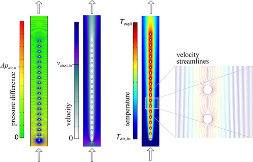
The contour lines of pressure difference next to the first few wires are very dense. In the middle part of the structure, the contour lines resemble each other and are less dense. Similar behavior can be seen for the velocity: a strongly changing velocity profile for the first wires and an almost unchanged profile in the middle. Both plots show the evolution of a hydraulically developed flow. The temperature profile shows no convergent behavior. This is due to the fact that a thermally developed flow is not defined by a nonvarying temperature profile in flow direction, but by a steady relation of local heat transfer rate to driving temperature difference between fluid and wall. The staggered arrangement shows in principle the same behavior.

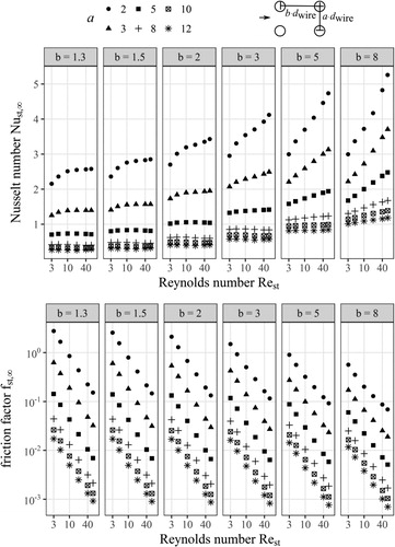
Nusselt numbers and Fanning friction factors for the developed flow are shown as functions of Reynolds number in Figure 7. Decreasing values of lateral distance $a$ yield higher Nusselt numbers and higher friction factors. Higher Nusselt numbers can be achieved with higher values of longitudinal distance $b$ and higher Reynolds number. The friction factor shows a linear relation with the Reynolds number in the logarithmic scale of Figure 7 for fixed geometry parameters. Each simulation point in Figure 7 is based on a parameter sweep of the number of wires from 2 up to 200 wires in flow direction (cf. Table 1).

Figure 7. Nusselt number and Fanning friction factor of an in-line wire structure for a developed flow as a function of Reynolds number and geometry parameters $a$ and $b$.

3.3. Determination of correlation

3.3.1. The effect of the number of wires

An exemplary set of results for one of the parameter sweeps defined in Table 1 is given in Figure 8 for the Nusselt number. It shows the results for the global Nusselt number ${\text{Nu}}_{\text{st}}$ from nine CFD simulations with fixed$\mathrm{ }a$, $b$, and ${\text{Re}}_{\text{st}}$ and varying number of wires. Based on Eq. (13)(13) $${\text{Nu}}_{\mathrm{s}\mathrm{t},y^{\mathrm{*}}}=\mathrm{N}{\mathrm{u}}_{\mathrm{s}\mathrm{t},\mathrm{\infty }}+\frac{C_{1,\mathrm{N}\mathrm{u}}}{C_{2,\mathrm{N}\mathrm{u}}{(y}^{\mathrm{*}}-1)}\left(1-{y^{\mathrm{*}}}^{{-C}_{2,\mathrm{N}\mathrm{u}}}\right)\mathrm{ }$$(13) , the Nusselt number ${\text{Nu}}_{\mathrm{s}\mathrm{t},\mathrm{\infty }}$ and the coefficients$\mathrm{ }{C}_{1,\mathrm{N}\mathrm{u}}$ and $C_{2,\mathrm{N}\mathrm{u}}$ were determined with a weighted least square error method. The weighting factor was chosen as the number of wires to the power of 3 to force good agreement of interpolation with the simulation for larger number of wires. The coefficients were used to express the local Nusselt number ${\text{Nu}}_{\mathrm{s}\mathrm{t},\text{local}}$ and the nondimensional thermal entrance length $L_{\text{th}}^{\mathrm{*}}$ in terms of Eqs. (14)(14) $${\text{Nu}}_{\mathrm{s}\mathrm{t},{\text{local},y}^{\mathrm{*}}}=\mathrm{N}{\mathrm{u}}_{\mathrm{s}\mathrm{t},\mathrm{\infty }}+C_{1,\mathrm{N}\mathrm{u}}{y^{\mathrm{*}}}^{-(C_{2,\mathrm{N}\mathrm{u}}+1)\mathrm{ }}$$(14) and (18)(18) $$L_{\text{th}}^{\mathrm{*}}={\left(\frac{\mathrm{N}{\mathrm{u}}_{\mathrm{s}\mathrm{t},\mathrm{\infty }}\mathrm{ }ϵ}{C_{1,\mathrm{N}\mathrm{u}}\left(1-ϵ\right)}\right)}^{-1/{(C}_{2,\mathrm{N}\mathrm{u}}+1)}$$(18) , respectively, both shown in Figure 8.

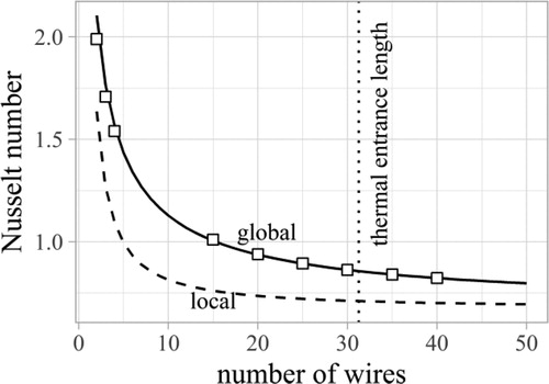
Figure 8. Correlated global (solid line) and local (dashed line) Nusselt number, ${\text{Nu}}_{\text{st}}$ and ${\text{Nu}}_{\mathrm{s}\mathrm{t},\text{local}}$, respectively, for an in-line wire arrangement, as a function of the number of wires based on the simulated global data points (squares) for ${\text{Nu}}_{\text{st}}$ and fixed values for$\mathrm{ }a=10,b=3,{\text{Re}}_{\text{st}}=20$. Downstream of the thermal entrance length (dotted line), the flow is declared as thermally developed.

The same procedure is followed for the friction factor. An exemplarily result is shown in Figure 9. The differences of the predicted values $\mathrm{N}{\mathrm{u}}_{\mathrm{s}\mathrm{t},{\mathrm{y}}^{\mathrm{*}},\text{corr}}$ and $f_{\mathrm{s}\mathrm{t},{\mathrm{y}}^{\mathrm{*}},\text{corr}}$ versus the simulated values $\mathrm{N}{\mathrm{u}}_{\mathrm{s}\mathrm{t},{\mathrm{y}}^{\mathrm{*}},\text{sim}}$ and $f_{\mathrm{s}\mathrm{t},{\mathrm{y}}^{\mathrm{*}},\text{sim}}$ based on Eq. 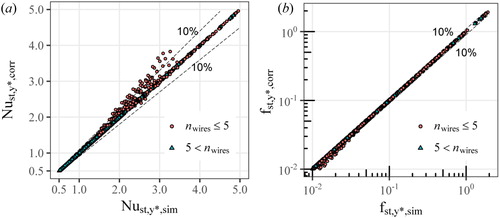(13)(13) $${\text{Nu}}_{\mathrm{s}\mathrm{t},y^{\mathrm{*}}}=\mathrm{N}{\mathrm{u}}_{\mathrm{s}\mathrm{t},\mathrm{\infty }}+\frac{C_{1,\mathrm{N}\mathrm{u}}}{C_{2,\mathrm{N}\mathrm{u}}{(y}^{\mathrm{*}}-1)}\left(1-{y^{\mathrm{*}}}^{{-C}_{2,\mathrm{N}\mathrm{u}}}\right)\mathrm{ }$$(13) are shown in Figure 10. The correlation shows errors of up to 20% for a low number of wires and equal or less than 1% for a number of wires higher than 5. 98% of the data are below a 10% relative residual error. A similar agreement is found for the correlation-based prediction of the friction factor.

Figure 9. Correlated global (solid line) and local (dashed line) friction factor,$\mathrm{ }{\mathrm{f}}_{\text{st}}$ and ${\mathrm{f}}_{\mathrm{s}\mathrm{t},\text{local}}$, respectively, for an in-line wire arrangement as a function of the number of wires based on the simulated global data points (squares) for ${\mathrm{f}}_{\text{st}}$ and fixed values for$\mathrm{ }a=10,b=3,{\text{Re}}_{\text{st}}=20$. Downstream of hydraulic entrance length (dotted line), the flow is declared as hydraulically developed; in-line arrangement.

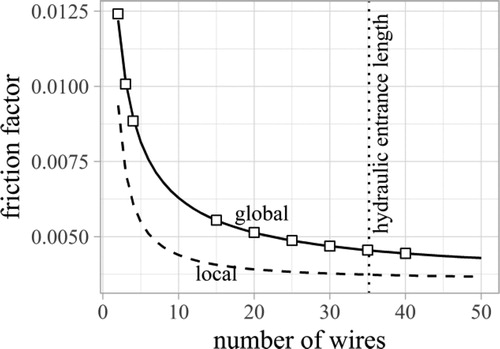
Figure 10. Predicted (correlated) values versus simulated values for (a) the Nusselt number ${\text{Nu}}_{\mathrm{s}\mathrm{t},y^{\mathrm{*}}}$ and (b) the Fanning friction factor $f_{\mathrm{s}\mathrm{t},y^{\mathrm{*}}}$. Data are based on Eqs. (13)(13) $${\text{Nu}}_{\mathrm{s}\mathrm{t},y^{\mathrm{*}}}=\mathrm{N}{\mathrm{u}}_{\mathrm{s}\mathrm{t},\mathrm{\infty }}+\frac{C_{1,\mathrm{N}\mathrm{u}}}{C_{2,\mathrm{N}\mathrm{u}}{(y}^{\mathrm{*}}-1)}\left(1-{y^{\mathrm{*}}}^{{-C}_{2,\mathrm{N}\mathrm{u}}}\right)\mathrm{ }$$(13) and (19)(19) $$f_{\mathrm{s}\mathrm{t},y^{\mathrm{*}}}=f_{\mathrm{s}\mathrm{t},\mathrm{\infty }}+\frac{C_{1,f}}{C_{2,f}{(y}^{\mathrm{*}}-1)}\left(1-{y^{\mathrm{*}}}^{{-C}_{2,f}}\right)\mathrm{ }$$(19) . The predicted values are correlated via the number of wires $n_{\text{wires}}$ (see Table 1) for specific Reynolds numbers ${\text{Re}}_{\text{st}}$ and geometry parameters $a$ and $b$ for an in-line arrangement.

3.3.2. The effect of Reynolds number and wire distances

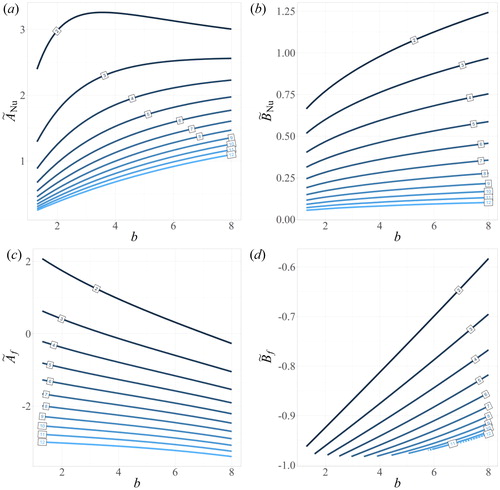
The Nusselt number $\mathrm{N}{\mathrm{u}}_{\mathrm{s}\mathrm{t},\mathrm{\infty }}$, Fanning friction factor $f_{\mathrm{s}\mathrm{t},\mathrm{\infty }}$, and the coefficients $C_{1,\mathrm{N}\mathrm{u}}$, $C_{2,\mathrm{N}\mathrm{u}}$, $C_{1,f}$, and $C_{2,f}$ were determined based on 216 different operating and geometry conditions (${\text{Re}}_{\text{st}},\mathrm{ }a,\mathrm{ }b$). Each coefficient is correlated to these conditions by means of a weighted least square error with the software Eureqa. The weighting factor is chosen as the reciprocal of the coefficient itself. Tables 3 and 4 give an overview of the derived correlations. Those correlations are chosen to be as accurate as possible, but with a limited number of correlation coefficients.

Table 3. Derived correlations for $\mathrm{N}{\mathrm{u}}_{\mathrm{s}\mathrm{t},\mathrm{\infty }}$ and ${\mathrm{f}}_{\mathrm{s}\mathrm{t},\mathrm{\infty }}$ for an in-line wire structure.

Coefficients	Auxiliary coefficients
$\mathrm{N}{\mathrm{u}}_{\mathrm{s}\mathrm{t},\mathrm{\infty }}={\tilde{A}}_{\text{Nu}}+0.021\mathrm{ }{\text{Re}}_{\text{st}}^{{\tilde{B}}_{\text{Nu}}}$	${\tilde{A}}_{\text{Nu}}=\mathrm{ }\frac{2.16\mathrm{ }b}{a\mathrm{ }+\mathrm{ }b\mathrm{ }-\mathrm{ }{\left(\frac{7.68\mathrm{ }b}{{\left(3.56\mathrm{ }+\mathrm{ }b\right)}^{0.5}}\right)}^{0.5}}$ ${\tilde{B}}_{\text{Nu}}=\frac{b^{0.345}}{\text{exp}\left(0.25\mathrm{ }a\right)\mathrm{ }}$
$f_{\mathrm{s}\mathrm{t},\mathrm{\infty }}=\text{exp}\left({\tilde{A}}_f+{\tilde{B}}_f\log \left(\mathrm{R}{\mathrm{e}}_{\text{st}}\right)\right)$	${\tilde{A}}_f=0.005531\mathrm{ }a\mathrm{ }b\mathrm{ }+\mathrm{ }0.005751\mathrm{ }{a}^2\mathrm{ }+\frac{8.6054\mathrm{ }-\mathrm{ }0.2222\mathrm{ }b}{a\mathrm{ }+\mathrm{ }0.1311\mathrm{ }a\mathrm{ }b}\mathrm{ }-\mathrm{ }0.9024\mathrm{ }-\mathrm{ }0.2985\mathrm{ }a\mathrm{ }-0.008528\mathrm{ }{b}^2$ ${\tilde{B}}_f=0.07776\mathrm{ }b\mathrm{ }+\mathrm{ }0.01624\mathrm{ }a\mathrm{ }+\mathrm{ }0.0001427\mathrm{ }a\mathrm{ }{b}^2\mathrm{ }-0.06345\mathrm{ }\log \left(a\right)-0.03442b\log \left(a\right)-1.02134$

Table 4. Derived correlations for coefficients of ${\text{Nu}}_{\text{st}}$ and ${\mathrm{f}}_{\text{st}}$ for in-line wire structure based on the Eqs. (13)(13) $${\text{Nu}}_{\mathrm{s}\mathrm{t},y^{\mathrm{*}}}=\mathrm{N}{\mathrm{u}}_{\mathrm{s}\mathrm{t},\mathrm{\infty }}+\frac{C_{1,\mathrm{N}\mathrm{u}}}{C_{2,\mathrm{N}\mathrm{u}}{(y}^{\mathrm{*}}-1)}\left(1-{y^{\mathrm{*}}}^{{-C}_{2,\mathrm{N}\mathrm{u}}}\right)\mathrm{ }$$(13) and (19)(19) $$f_{\mathrm{s}\mathrm{t},y^{\mathrm{*}}}=f_{\mathrm{s}\mathrm{t},\mathrm{\infty }}+\frac{C_{1,f}}{C_{2,f}{(y}^{\mathrm{*}}-1)}\left(1-{y^{\mathrm{*}}}^{{-C}_{2,f}}\right)\mathrm{ }$$(19) .

Coefficients	Auxiliary coefficients
$C_{1,\mathrm{N}\mathrm{u}}=\mathrm{ }\begin{array}{c}{\tilde{A}}_{1,\mathrm{N}\mathrm{u}}\text{ if }{\text{Re}}_{\text{st}}^{0.8}{a}^{2.0}{b}^{-1.1}>24\\ 0\text{ if }{\text{Re}}_{\text{st}}^{0.8}{a}^{2.0}{b}^{-1.1}\le 24\end{array}$	${\tilde{A}}_{1,\mathrm{N}\mathrm{u}}=1.6896\mathrm{ }+\mathrm{ }0.03636\mathrm{ }b\mathrm{ }+\mathrm{ }0.02745\mathrm{ }\mathrm{R}{\mathrm{e}}_{\text{st}}+\mathrm{ }\frac{0.5171\mathrm{ }a\mathrm{ }\mathrm{N}{\mathrm{u}}_{\mathrm{s}\mathrm{t},\mathrm{\infty }}}{b}\mathrm{ }+\mathrm{ }\frac{-4.4822}{2.0963\mathrm{ }+\mathrm{ }0.1266\mathrm{ }\mathrm{R}{\mathrm{e}}_{\text{st}}}\mathrm{ }-\mathrm{ }0.6369\mathrm{ }\mathrm{N}{\mathrm{u}}_{\mathrm{s}\mathrm{t},\mathrm{\infty }}$
$C_{1,f}=\mathrm{ }\begin{array}{c}{\tilde{A}}_{1,f}\text{ if }R{e}_{st}^{0.8}{a}^{1.8}{b}^{-1.0}>12\\ 0\text{ if }R{e}_{st}^{0.8}{a}^{1.8}{b}^{-1.0}\le 12\end{array}$	${\tilde{A}}_{1,f}=2.9\cdot {10}^{-5}\mathrm{ }-\mathrm{ }0.428\mathrm{ }{f}_{\mathrm{s}\mathrm{t},\mathrm{\infty }}\mathrm{ }+\frac{f_{\mathrm{s}\mathrm{t},\mathrm{\infty }}^{0.5}}{{\tilde{B}}_{1,f}}$ ${\tilde{B}}_{1,f}=1.631\mathrm{ }b\mathrm{ }+\mathrm{ }0.064\mathrm{ }a\text{ log}\left(\mathrm{R}{\mathrm{e}}_{\text{st}}\right)\mathrm{ }-\mathrm{ }0.62\mathrm{ }-\mathrm{ }0.0562\mathrm{ }a\mathrm{ }{b}^{0.5}-\mathrm{ }0.155\mathrm{ }b\text{ log}\left(\mathrm{R}{\mathrm{e}}_{\text{st}}\right)$
$C_2={\mathrm{C}}_{2,f}=C_{2,\mathrm{N}\mathrm{u}}=\frac{1}{1+{\tilde{A}}_2}$	${\tilde{A}}_2=3.77\cdot {10}^{-6}\mathrm{ }{\text{Re}}_{\text{st}}^{1.95}\mathrm{ }{a}^{3.81}\mathrm{ }{b}^{-0.68}$

The Nusselt number $\mathrm{N}{\mathrm{u}}_{\mathrm{s}\mathrm{t},\mathrm{\infty }}\mathrm{ }$is related to the Reynolds number by a power law ansatz. The exponent varies between 0.1 and 1.25 mainly dependent on the lateral wire distance $a$. Figures 11a and b show the shape of curve for ${\tilde{A}}_{\text{Nu}}$ and for the exponent ${\tilde{B}}_{\text{Nu}}\mathrm{ }$based on both geometry parameters. The friction factor $f_{\mathrm{s}\mathrm{t},\mathrm{\infty }}\mathrm{ }$is related to the logarithm of the Reynolds number by an exponential ansatz. The auxiliary coefficients ${\tilde{A}}_f$ and ${\tilde{B}}_f$ are shown in Figures 11c and d, respectively. Both approaches, the power law ansatz and the exponential ansatz, are widely used to correlate the Nusselt number and the Fanning friction factor to the Reynolds number, respectively [11].

Figure 11. Auxiliary coefficients$\mathrm{ }{\tilde{A}}_{\text{Nu}}\mathrm{ }$(a), ${\tilde{B}}_{\text{Nu}}$ (b), ${\tilde{A}}_f$ (c), and ${\tilde{B}}_f$ (d) needed for calculation of correlated Nusselt number and friction factor based on Table 3 for in-line arrangement. Geometry parameter $a$ is shown on the contour lines.

The coefficients $C_{1,\mathrm{N}\mathrm{u}}$ and $C_{1,f}$ are set to zero in case the global Nusselt number and friction factor, respectively, depend only weakly on the number of wires. Otherwise they are related to the operating and geometry conditions, as well as to $\mathrm{N}{\mathrm{u}}_{\mathrm{s}\mathrm{t},\mathrm{\infty }}\mathrm{ }$and $f_{\mathrm{s}\mathrm{t},\mathrm{\infty }}$.

Finally, the coefficient $C_2\mathrm{ }$as a representative of the decay of Nusselt number and friction factor with respect to the number of wires was chosen equal for both the thermal and the hydraulic decay.

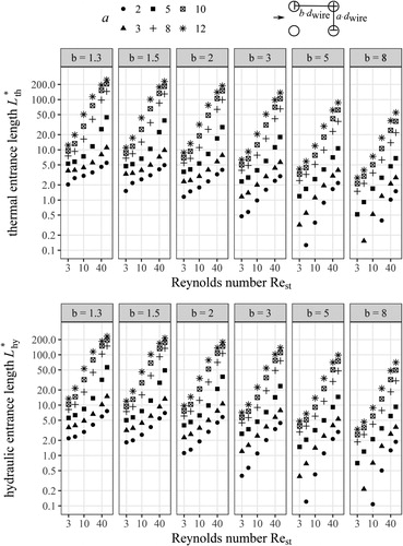
In Figure 12, the nondimensional thermal and hydraulic entrance length is shown. Increasing Reynolds number, increasing lateral wire distance $a$, and decreasing longitudinal wire distance $b$ yield a higher thermal entrance length. The entrance lengths range from 1 wire up to 200 wires. The correlations in Tables 3 and 4 can be used to calculate the entrance lengths $L_{\text{th}}^{\mathrm{*}}$ and $L_{\text{hy}}^{\mathrm{*}}$ based on the Eqs. (18)(18) $$L_{\text{th}}^{\mathrm{*}}={\left(\frac{\mathrm{N}{\mathrm{u}}_{\mathrm{s}\mathrm{t},\mathrm{\infty }}\mathrm{ }ϵ}{C_{1,\mathrm{N}\mathrm{u}}\left(1-ϵ\right)}\right)}^{-1/{(C}_{2,\mathrm{N}\mathrm{u}}+1)}$$(18) and (21)(21) $$L_{\text{hy}}^{\mathrm{*}}={\left(\frac{f_{\mathrm{s}\mathrm{t},\mathrm{\infty }}\mathrm{ }ϵ}{C_{1,f}\left(1-ϵ\right)}\right)}^{-1/(C_{2,f}+1)}$$(21) , respectively.

Figure 12. Nondimensional entrance lengths $L_{\text{th}}^{\mathrm{*}}$ and $L_{\text{hy}}^{\mathrm{*}}\mathrm{ }$for an in-line arrangement based on the Reynolds number ${\text{Re}}_{\text{st}}$ and geometry parameters $a$ and $b$. Entrances lengths below 0.1 are not shown.

3.4. Correlation error

The correlations show good agreement for all investigated parameters$\mathrm{ }a$,$\mathrm{ }b,$ and $\mathrm{R}{\mathrm{e}}_{\text{st}}$. The corresponding differences are summarized in Figures 13 and 14 for ${\text{Nu}}_{\mathrm{s}\mathrm{t},\mathrm{\infty }}$, $f_{\mathrm{s}\mathrm{t},\mathrm{\infty }}$ and for ${\text{Nu}}_{\mathrm{s}\mathrm{t},{\mathrm{y}}^{\mathrm{*}}}$, $f_{\mathrm{s}\mathrm{t},{\mathrm{y}}^{\mathrm{*}}}$, respectively.

Figure 13. Predicted (correlated) values versus simulated values for (a) the Nusselt number ${\text{Nu}}_{\mathrm{s}\mathrm{t},\mathrm{\infty }}$ and (b) the Fanning friction factor ${\mathrm{f}}_{\mathrm{s}\mathrm{t},\mathrm{\infty }}$ for a developed flow. Data are based on Table 3. The predicted values are correlated via the Reynolds number ${\text{Re}}_{\text{st}}$ and geometry parameters $a$ and $b$ for an in-line wire arrangement.

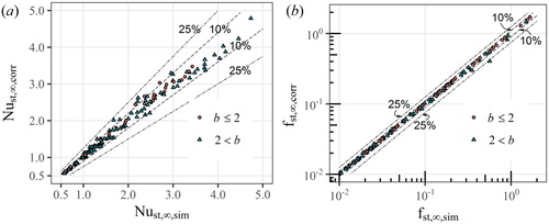
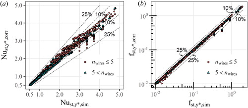
Figure 14. Predicted (correlated) values versus simulated values for (a) the Nusselt number ${\text{Nu}}_{\mathrm{s}\mathrm{t},{\mathrm{y}}^{\mathrm{*}}}$ and (b) the Fanning friction factor ${\mathrm{f}}_{\mathrm{s}\mathrm{t},y^{\mathrm{*}}}$. Data are based on Eqs. (13)(13) $${\text{Nu}}_{\mathrm{s}\mathrm{t},y^{\mathrm{*}}}=\mathrm{N}{\mathrm{u}}_{\mathrm{s}\mathrm{t},\mathrm{\infty }}+\frac{C_{1,\mathrm{N}\mathrm{u}}}{C_{2,\mathrm{N}\mathrm{u}}{(y}^{\mathrm{*}}-1)}\left(1-{y^{\mathrm{*}}}^{{-C}_{2,\mathrm{N}\mathrm{u}}}\right)\mathrm{ }$$(13) and (19)(19) $$f_{\mathrm{s}\mathrm{t},y^{\mathrm{*}}}=f_{\mathrm{s}\mathrm{t},\mathrm{\infty }}+\frac{C_{1,f}}{C_{2,f}{(y}^{\mathrm{*}}-1)}\left(1-{y^{\mathrm{*}}}^{{-C}_{2,f}}\right)\mathrm{ }$$(19) (Tables 3 and 4). The predicted values are correlated via the Reynolds number ${\text{Re}}_{\text{st}}$, geometry parameters $a$ and $b$, and the number of wires for an in-line wire arrangement.

It can be seen that the relative differences of predicted (correlated) Nusselt numbers versus simulated Nusselt numbers are below 25% and similarly for friction factors. The correlation predicts 94% and 99% of the simulated data for ${\text{Nu}}_{\mathrm{s}\mathrm{t},\mathrm{\infty }}$ and $f_{\mathrm{s}\mathrm{t},\mathrm{\infty }}$ within ±10%, respectively. Therefore, a thermally and hydraulically developed flow is well predicted with the correlation. The developing flows have an additional dependency on the number of wires. The correlation for the developing flow predicts 93% and 97% of the simulated data for ${\text{Nu}}_{\mathrm{s}\mathrm{t},{\mathit{y}}^{\mathrm{*}}}$ and $f_{\mathrm{s}\mathrm{t},{\mathit{y}}^{\mathrm{*}}}$ within ±10%, respectively. Table 5 shows details of the relative residual errors for different intervals and number of wires.

Table 5. Percentage of correlated data which satisfy a relative residual error below 5% and 10% for ${\text{Nu}}_{\mathrm{s}\mathrm{t},\mathrm{\infty }}$, ${\mathrm{f}}_{\mathrm{s}\mathrm{t},\mathrm{\infty }}$,$\mathrm{ }{\text{Nu}}_{\mathrm{s}\mathrm{t},{\mathrm{y}}^{\mathrm{*}}}$, and ${\mathrm{f}}_{\mathrm{s}\mathrm{t},{\mathrm{y}}^{\mathrm{*}}}$.

		${\text{Nu}}_{\mathrm{s}\mathrm{t},\mathrm{\infty }}$	$f_{\mathrm{s}\mathrm{t},\mathrm{\infty }}$	${\text{Nu}}_{\mathrm{s}\mathrm{t},{\mathrm{y}}^{\mathrm{*}}}$		$f_{\mathrm{s}\mathrm{t},y^{\mathrm{*}}}$
		$n_{\text{wires}}$
		$>L_{\text{th}}^{\mathrm{*}}$	$>L_{\text{hy}}^{\mathrm{*}}$	$>2$	> 5	> 2	> 5
Relative residual error	<5%	81 %	94 %	76 %	79 %	89 %	92 %
	<10%	94 %	99 %	93 %	95 %	97 %	99 %

The percentage is specified for different number of wires in an in-line wire arrangement.

4. Discussion

The decrease in Nusselt number and friction factor for the in-line arrangement with respect to the number of wires can be well represented by the power law ansatz in Eqs. (13)(13) $${\text{Nu}}_{\mathrm{s}\mathrm{t},y^{\mathrm{*}}}=\mathrm{N}{\mathrm{u}}_{\mathrm{s}\mathrm{t},\mathrm{\infty }}+\frac{C_{1,\mathrm{N}\mathrm{u}}}{C_{2,\mathrm{N}\mathrm{u}}{(y}^{\mathrm{*}}-1)}\left(1-{y^{\mathrm{*}}}^{{-C}_{2,\mathrm{N}\mathrm{u}}}\right)\mathrm{ }$$(13) and (19)(19) $$f_{\mathrm{s}\mathrm{t},y^{\mathrm{*}}}=f_{\mathrm{s}\mathrm{t},\mathrm{\infty }}+\frac{C_{1,f}}{C_{2,f}{(y}^{\mathrm{*}}-1)}\left(1-{y^{\mathrm{*}}}^{{-C}_{2,f}}\right)\mathrm{ }$$(19) for each combination of geometry parameters $a$ and $b$, and the operation parameter Reynolds number (cf. Figures 8 and 9). The derived correlation for the developing flow predicts 93% and 97% of the simulated data for ${\text{Nu}}_{\mathrm{s}\mathrm{t},{\mathit{y}}^{\mathrm{*}}}$ and $f_{\mathrm{s}\mathrm{t},{\mathit{y}}^{\mathrm{*}}}$ within ±10%. For the fully developed flow, the correlation predicts 94% and 99% of the simulated data for ${\text{Nu}}_{\mathrm{s}\mathrm{t},\mathrm{\infty }}$ and $f_{\mathrm{s}\mathrm{t},\mathrm{\infty }}$ within ±10%. Further, the power law ansatz allows a description of the hydraulic and thermal entrance length related to$\mathrm{ }a$, $b$, and $\mathrm{R}{\mathrm{e}}_{\text{st}}$. The strong increase in nondimensional entrance length with decreasing $b$ can be explained by a shadowing effect for serried rows of wires in flow direction. A change in Reynolds numbers and lateral wire distances yields, similar to laminar fluid flow through a pipe, a proportional change in nondimensional entrance length [30]. Figure 12 affirms this statement. Table 4 shows a simplified relation among $a$, $b$, and $\mathrm{R}{\mathrm{e}}_{\text{st}}$ for which the entrance region can be neglected for performance evaluation. For this combination of parameters, it is sufficient to use the Nusselt number ${\text{Nu}}_{\mathrm{s}\mathrm{t},\mathrm{\infty }}$ and friction factor $f_{\mathrm{s}\mathrm{t},\mathrm{\infty }}$ based on Table 3, independent of the number of wires in the application. However, apart from this combination of parameters, it is necessary to include the entrance region in the performance evaluation. The global Nusselt number for a specific heat exchanger can vary significantly from the Nusselt number ${\text{Nu}}_{\mathrm{s}\mathrm{t},\mathrm{\infty }}$ derived for the developed flow. Especially for compact heat exchangers with dimensions in the submillimeter range, the structure length in flow direction $L_{\text{st}}$ is small, as heat transfer coefficients are high. Thus, the number of wires in flow direction can be very low and differ strongly from the nondimensionalized entrance lengths. Exemplarily Figure 8 shows the difference of global Nusselt number ${\text{Nu}}_{\mathrm{s}\mathrm{t},10}$ for a number of wires $n_{\text{wires}}=10$ to the Nusselt number ${\text{Nu}}_{\mathrm{s}\mathrm{t},\mathrm{\infty }}$ derived for the developed flow. ${\text{Nu}}_{\mathrm{s}\mathrm{t},10}$ is 1.7 times higher than ${\text{Nu}}_{\mathrm{s}\mathrm{t},\mathrm{\infty }}$.

Table B1. Predicted correlation for coefficients of ${\text{Nu}}_{\text{st}}$ and ${\mathrm{f}}_{\text{st}}$ for staggered wire structure based on the Eqs. (13)(13) $${\text{Nu}}_{\mathrm{s}\mathrm{t},y^{\mathrm{*}}}=\mathrm{N}{\mathrm{u}}_{\mathrm{s}\mathrm{t},\mathrm{\infty }}+\frac{C_{1,\mathrm{N}\mathrm{u}}}{C_{2,\mathrm{N}\mathrm{u}}{(y}^{\mathrm{*}}-1)}\left(1-{y^{\mathrm{*}}}^{{-C}_{2,\mathrm{N}\mathrm{u}}}\right)\mathrm{ }$$(13) and (19)(19) $$f_{\mathrm{s}\mathrm{t},y^{\mathrm{*}}}=f_{\mathrm{s}\mathrm{t},\mathrm{\infty }}+\frac{C_{1,f}}{C_{2,f}{(y}^{\mathrm{*}}-1)}\left(1-{y^{\mathrm{*}}}^{{-C}_{2,f}}\right)\mathrm{ }$$(19) .

Coefficients	Auxiliary coefficients
${\text{Nu}}_{\mathrm{s}\mathrm{t},\mathrm{\infty }}={\tilde{A}}_{\text{Nu}}+0.021\mathrm{ }{\text{Re}}_{\text{st}}^{{\tilde{B}}_{\text{Nu}}}$	${\tilde{A}}_{\text{Nu}}=\mathrm{ }0.91\mathrm{ }+\frac{2.57}{b}\mathrm{ }+\mathrm{ }\frac{2.2\mathrm{ }-\mathrm{ }0.78a}{\text{exp}\left(b\right)}$ ${\tilde{B}}_{\text{Nu}}=0.598\mathrm{ }+\mathrm{ }0.065\mathrm{ }\frac{a}{b}\mathrm{ }-\mathrm{ }0.393{\left(\frac{a}{b}\right)}^{0.5}$
$f_{\mathrm{s}\mathrm{t},\mathrm{\infty }}=\text{exp}\left({\tilde{A}}_f+{\tilde{B}}_f\log \left(\mathrm{R}{\mathrm{e}}_{\text{st}}\right)\right)$	${\tilde{A}}_f=1.28\mathrm{ }+\mathrm{ }0.62\mathrm{ }\frac{b}{a}\mathrm{ }+\frac{4.31\mathrm{ }-\mathrm{ }2.05\mathrm{ }{\left(a\right)}^{0.5}}{b}\mathrm{ }-\mathrm{ }0.015\mathrm{ }a\mathrm{ }-\mathrm{ }2.06\text{ log}\left(b\right)$ ${\tilde{B}}_f=-\frac{1.43}{b}\mathrm{ }+\frac{2.65}{a\mathrm{ }b}\mathrm{ }+\mathrm{ }0.078\frac{a}{b^2}\mathrm{ }-\mathrm{ }0.297\mathrm{ }-\mathrm{ }b\mathrm{ }{0.23}^a\mathrm{ }-\mathrm{ }0.025\mathrm{ }a$
$C_{1,\mathrm{N}\mathrm{u}}=\mathrm{ }\begin{array}{ll}{\tilde{A}}_{1,\mathrm{N}\mathrm{u}}& \text{if }{\text{Re}}_{\text{st}}^{0.9}{a}^{2.4}{b}^{-1.2}>240\\ 0& \text{if }{\text{Re}}_{\text{st}}^{0.9}{a}^{2.4}{b}^{-1.2}\le 240\end{array}$	${\tilde{A}}_{1,\mathrm{N}\mathrm{u}}=0.22\mathrm{ }+\mathrm{ }0.16\mathrm{ }\mathrm{R}{\mathrm{e}}_{\text{st}}+\frac{0.89}{b}+\mathrm{ }0.02\mathrm{ }a\mathrm{ }b\mathrm{ }+\mathrm{ }0.000045\mathrm{ }\mathrm{R}{\mathrm{e}}_{\text{st}}^3-\mathrm{ }0.35\mathrm{ }b\mathrm{ }-\mathrm{ }0.0021\mathrm{ }\mathrm{R}{\mathrm{e}}_{\text{st}}^2-\mathrm{ }0.2{\text{ Nu}}_{\mathrm{s}\mathrm{t},\mathrm{\infty }}^2$
$C_{1,f}=\mathrm{ }\begin{array}{cc}{\tilde{A}}_{1,\mathrm{f}}& \text{if }\mathrm{R}{\mathrm{e}}_{st}^{0.9}{a}^{2.2}{b}^{-1.1}>255\\ 0& \text{if }\mathrm{R}{\mathrm{e}}_{\mathrm{s}\mathrm{t}}^{0.9}{a}^{2.2}{b}^{-1.1}\le 255\end{array}$	${\tilde{A}}_{1,f}=f_{\mathrm{s}\mathrm{t},\mathrm{\infty }}\mathrm{ }\left[0.15\mathrm{ }\mathrm{R}{\mathrm{e}}_{\text{st}}^{0.5}-\frac{4.97}{a}\mathrm{ }+\mathrm{ }\frac{0.017\mathrm{ }a{\mathrm{ }\left(0.87\mathrm{ }+\mathrm{ }\mathrm{R}{\mathrm{e}}_{\text{st}}\right)}^{0.5}{\left(13.85\text{ log}\left(a\right)\right)}^{0.5}}{b}\mathrm{ }-\mathrm{ }0.46\right]\mathrm{ }$
$C_{2,\mathrm{N}\mathrm{u}}=\mathrm{ }\frac{1.20}{1+{\tilde{A}}_{2,\mathrm{N}\mathrm{u}}}$	${\tilde{A}}_{2,\mathrm{N}\mathrm{u}}=3.070\cdot {10}^{-4}\mathrm{ }{\text{Re}}_{\text{st}}^{0.886}\mathrm{ }{a}^{2.719}\mathrm{ }{b}^{-0.928}$
$C_{2,f}=\mathrm{ }\frac{1.01}{1+{\tilde{A}}_{2,f}}$	${\tilde{A}}_{2,f}=3.286\cdot {10}^{-6}\mathrm{ }{\text{Re}}_{\text{st}}^{1.448}\mathrm{ }{a}^{3.842}\mathrm{ }{b}^{-1.260}$

Correlation is valid for:$\mathrm{ }3\le a\le 12$,$\mathrm{ }1.3\le b\le 8$,$\text{ and }3\le \mathrm{R}{\mathrm{e}}_{\text{st}}\le 60$.

Table B2. Percentage of correlated data which satisfy a relative residual error below 5% and 10% for ${\text{Nu}}_{\mathrm{s}\mathrm{t},\mathrm{\infty }}$, ${\mathrm{f}}_{\mathrm{s}\mathrm{t},\mathrm{\infty }}$,$\mathrm{ }{\text{Nu}}_{\mathrm{s}\mathrm{t},{\mathrm{y}}^{\mathrm{*}}}$, and ${\mathrm{f}}_{\mathrm{s}\mathrm{t},{\mathrm{y}}^{\mathrm{*}}}\mathrm{ }$in staggered wire arrangement.

		${\text{Nu}}_{\mathrm{s}\mathrm{t},\mathrm{\infty }}$	$f_{\mathrm{s}\mathrm{t},\mathrm{\infty }}$	${\text{Nu}}_{\mathrm{s}\mathrm{t},{\mathrm{y}}^{\mathrm{*}}}$		$f_{\mathrm{s}\mathrm{t},y^{\mathrm{*}}}$
		$n_{\text{wires}}$
		$>L_{\text{th}}^{\mathrm{*}}$	$>L_{\text{hy}}^{\mathrm{*}}$	$>2$	> 5	> 2	> 5
Relative residual error $3\le a\le 12$	<5%	67	71	68	68	68	69
	<10%	90	89	92	91	87	88
Relative residual error $5\le a\le 12$	<5%	70	80	73	74	78	79
	<10%	88	95	91	90	95	95

The percentage is specified for different number of wires. Correlation is valid for: $3\le a\le 12$, $1.3\le b\le 8$, and $3\le \mathrm{R}{\mathrm{e}}_{\text{st}}\le 60$.

The correlation predicts a number of wires in the range of 2–5 more inexact than higher number of wires. This decline in predictability is due to an error-prone estimation for low number of wires based on the method of interpolation. Therefore, it is recommended using the correlation for a number of wires less than 5 with caution. However, this restriction is minor, as a wire structure heat exchanger will probably be manufactured with more than five wires in flow direction in order to achieve a sufficiently high heat transfer surface.

The performance upscaling to a 3D wire structure heat exchanger needs in addition information on wire material (particularly thermal conductivity) and wire length. Based on this information, the fin efficiency [11] can be calculated and combined with the heat transfer coefficient calculated from the correlation given in this article. Assuming the wire structure surface area dominates the total heat transfer surface area, the thermal resistance on the air side can then be calculated. This procedure is valid as long as the influence of the tube wall is negligibly small (cf. model assumption AS4). Thus, very open structures (large $a$ and $b$) or structures with short wire lengths need information on heat transfer on the outer tube wall.

The staggered arrangement (with correlations shown in the Appendix) shows higher Nusselt numbers and friction factors compared to the in-line arrangement for the same Reynolds number and geometry parameters $a$ and $b$. This is not surprising, as the blockage of flow in the staggered arrangement is obvious. Thus, a staggered arrangement allows an even more compact design than the in-line arrangement. However, the related increase in pressure drop has to be considered.

5. Conclusions

Within this study, correlation functions for the Nusselt number and the Fanning friction factor are developed. They hold for a laminar flow in an in-line and staggered array of circular cylinders. The dimensions and operating conditions are guided by wire structure heat exchangers, in particular with extended surfaces such as micro-pin fins and textile structures. The derived correlation is a function of the Reynolds number, the wire distances, and the number of wires. The Reynolds number $\mathrm{R}{\mathrm{e}}_{\text{st}}$ varies from 3 to 60, the lateral wire distance $a$ from 2 to 12, and the longitudinal wire distance $b$ from 1.3 to 8. The number of wires is not restricted. The power law ansatz describing the shape of curve for the Nusselt number and the friction factor with respect to the number of wires shows very good agreement of correlation with simulated data for the stated range of parameters. The power law ansatz for the in-line arrangement can predict more than 95% of the simulated data within ±5%. In order to use this ansatz for varying Reynolds numbers and wire distances, the coefficients of the power law ansatz have to be correlated to the stated three parameters ${\text{Re}}_{\text{st}},\mathrm{ }a$, and$\mathrm{ }b$. Thus, a correlation of Nusselt number and Fanning friction factor with respect to all four parameters$\mathrm{ }{\text{Re}}_{\text{st}},\mathrm{ }a$, $b$, and $n_{\text{wires}}$ is derived. This correlation shows slightly less agreement. The correlation for the developed flow can predict 81% and 94% of the simulated data for ${\text{Nu}}_{\mathrm{s}\mathrm{t},\mathrm{\infty }}$ and $f_{\mathrm{s}\mathrm{t},\mathrm{\infty }}$ within ±5%. For the developing flow with number of wires larger than 5, it can predict 79% and 92% of the simulated data for ${\text{Nu}}_{\mathrm{s}\mathrm{t},{\mathit{y}}^{\mathrm{*}}}$ and $f_{\mathrm{s}\mathrm{t},{\mathit{y}}^{\mathrm{*}}}$ within ±5%. Increasing the interval to ±10%, more than 95% can be predicted. Apart from the in-line arrangement of wires, correlations are developed for the staggered arrangement. Similar predictability can be achieved here.

The correlations are based on simulations. A comparison of the simulation with measurements data [18,21] shows acceptable agreement of Fanning friction factors and Nusselt numbers under the constraint of an irregular geometry.

It is recommended to use the correlation only within the specified range of parameters and to consider the inexact predictability for a number of wires below 5, and for a ratio of structure height to lateral wire distance below 5. The correlations are derived for engineers, who dimension and design pin fin and textile structure heat exchangers and need simplified tools for calculation of performance.

Nomenclature
$A^{\mathrm{\prime }}$	=	area projected to a line (m)
$\tilde{A}$	=	auxiliary coefficient for correlation
$a$	=	lateral wire distance (m)
$\tilde{B}$	=	auxiliary coefficient for correlation
$b$	=	longitudinal wire distance (m)
$\mathrm{B}\mathrm{r}$	=	Brinkman number (-)
$c$	=	coefficient for correlation
$c_p$	=	specific heat (J/kg·K)
$d$	=	diameter or characteristic length (m)
$f$	=	Fanning friction factor
$H$	=	height (m)
$h$	=	convection heat transfer coefficient (W/m2K)
I	=	identity
$k$	=	thermal conductivity (W/m K)
$L$	=	length (m)
$L^{\mathrm{*}}$	=	nondimensional entrance length
l	=	wire distance (m)
$n$	=	quantity
$\mathrm{N}\mathrm{u}$	=	Nusselt number
$\mathrm{P}\mathrm{r}$	=	Prandtl number
$p$	=	pressure (Pa)
$\dot{q}$	=	line heat flux (W/m)
$\mathrm{R}\mathrm{e}$	=	Reynolds number
$T$	=	temperature (K)
u	=	velocity field (m/s)
$v$	=	velocity in y-direction (m/s)
$y^{\mathrm{*}}$	=	nondimensional flow direction (cf. Eq. (12)(12) $$y^{\mathrm{*}}=\frac{y}{d_{\text{wire}}b}$$(12) )

Greek Symbols
$ϵ$	=	tolerated error
$\mu$	=	dynamic viscosity (Pa s)
ρ	=	density (kg/m³)

Subscripts
air	=	air side
eff	=	effective
HTS	=	heat transfer surface
HX	=	heat exchanger
hy	=	hydraulic
in	=	inlet
lat	=	lateral, perpendicular to the air flow direction
long	=	longitudinal, in air flow direction
local	=	related to a single wire
m	=	mean
out	=	outlet
st	=	domain between tubes for heat transfer enhancement structure
th	=	thermal
wires	=	related to all wires
wall	=	wall side
$\mathrm{\infty }$	=	fully developed flow

Acknowledgments

The results of this article have been developed within the project MinWaterCSP.

Additional information

Funding

This project has received funding from the European Union’s Horizon 2020 research and innovation program under grant agreement No. 654443.

Appendix

A. Definition of correlation for Fanning friction factor

(19) $$f_{\mathrm{s}\mathrm{t},y^{\mathrm{*}}}=f_{\mathrm{s}\mathrm{t},\mathrm{\infty }}+\frac{C_{1,f}}{C_{2,f}{(y}^{\mathrm{*}}-1)}\left(1-{y^{\mathrm{*}}}^{{-C}_{2,f}}\right)\mathrm{ }$$(19) (20) $$f_{\mathrm{s}\mathrm{t},{\text{local},y}^{\mathrm{*}}}=f_{\mathrm{s}\mathrm{t},\mathrm{\infty }}+C_{1,f}{y^{\mathrm{*}}}^{-(C_{2,f}+1)\mathrm{ }}$$(20) (21) $$L_{\text{hy}}^{\mathrm{*}}={\left(\frac{f_{\mathrm{s}\mathrm{t},\mathrm{\infty }}\mathrm{ }ϵ}{C_{1,f}\left(1-ϵ\right)}\right)}^{-1/(C_{2,f}+1)}$$(21)

B. Staggered arrangement

Table B1 and B2 show the predicted correlations and their residual errors, respectively.

References

- J. M. P. Q. Delgado, and H. a. Mass, Transfer in Porous Media. Berlin, Heidelberg: Springer-Verlag, 2012.
- C. Hutter, D. Büchi, V. Zuber, and P. Rudolf von Rohr, “Heat transfer in metal foams and designed porous media,” Chem. Eng. Sci., vol. 66, no. 17, pp. 3806–3814, 2011. DOI: 10.1016/j.ces.2011.05.005.
- K.-J. Kang, “Wire-woven cellular metals: The present and future,” Prog. Mater. Sci., vol. 69, pp. 213–307, 2015. DOI: 10.1016/j.pmatsci.2014.11.003.
- J. Tian et al., “The effects of topology upon fluid-flow and heat-transfer within cellular copper structures,” Int. J. Heat Mass Transfer, vol. 47, no. 14–16, pp. 3171–3186, 2004. DOI: 10.1016/j.ijheatmasstransfer.2004.02.010.
- K. Boomsma, D. Poulikakos, and F. Zwick, “Metal foams as compact high performance heat exchangers,” Mech. Mater., vol. 35, no. 12, pp. 1161–1176, 2003. DOI: 10.1016/j.mechmat.2003.02.001.
- D. Girlich, Grundsatzuntersuchungen Zum Einsatz Offenporiger Metallschäume in Der Luft-, Kälte- und Wärmetechnik. Lindenberg: Abschlussbericht, M-Pore GmbH, 2006.
- C. Marques, and K. W. Kelly, “Fabrication and performance of a pin fin micro heat exchanger,” J. Heat Transfer, vol. 126, no. 3, pp. 434–444, 2004. DOI: 10.1115/1.1731341.
- D. J. Sypeck, and H. N. G. Wadley, “Multifunctional microtruss laminates: Textile synthesis and properties,” J. Mater. Res., vol. 16, no. 03, pp. 890–897, 2001. DOI: 10.1557/JMR.2001.0117.
- I. Kotcioglu, G. Omeroglu, and S. Caliskan, “Thermal performance and pressure drop of different pin-fin geometries,” Hittite J. Sci. Eng., vol. 1, pp. 13–20, 2014. DOI: 10.17350/HJSE19030000003.
- N. Sahiti, A. Lemouedda, D. Stojkovic, F. Durst, and E. Franz, “Performance comparison of pin fin in-duct flow arrays with various pin cross-sections,” Appl. Therm. Eng., vol. 26, no. 11–12, pp. 1176–1192, 2006. DOI: 10.1016/j.applthermaleng.2005.10.042.
- R. K. Shah, and D. P. Sekulić, Fundamentals of Heat Exchanger Design, 1st ed. Hoboken, NJ: John Wiley & Sons, 2003.
- Y. Liu, G. Xu, X. Luo, H. Li, and J. Ma, “An experimental investigation on fluid flow and heat transfer characteristics of sintered woven wire mesh structures” Therm. Eng., vol. 80, pp. 118–126, 2015. DOI: 10.1016/j.applthermaleng.2015.01.050.
- J. Xu, J. Tian, T. J. Lu, and H. P. Hodson, “On the thermal performance of wire-screen meshes as heat exchanger material,” Int. J. Heat Mass Transfer, vol. 50, no. 5–6, pp. 1141–1154, 2007. DOI: 10.1016/j.ijheatmasstransfer.2006.05.044.
- S. B. Prasad, J. S. Saini, and K. M. Singh, “Investigation of heat transfer and friction characteristics of packed bed solar air heater using wire mesh as packing material,” Sol. Energy, vol. 83, no. 5, pp. 773–783, 2009. DOI: 10.1016/j.solener.2008.11.011.
- C. Li, and R. A. Wirtz, Development of a High Performance Heat Sink Based on Screen-Fin Technology. Reno, NV: University of Nevada, 2003.
- E. van Andel, Heat exchanger and method for manufacturing same, Patent EP0714500 B1, 1996.
- J. P. Bonestroo, “Calculation model of fine-wire heat exchanger,” Master Thesis, Twente University, Enschede, Netherlands, 2012.
- H. Fugmann, P. D. Lauro, and L. Schnabel, Heat Transfer Surface Area Enlargement by Usage of Metal Textile Structures – Development, Potential and Evaluation. Dresden: International Textile Conference, 2016. DOI: 10.3390/en10091341.
- N. Sahiti, “Thermal and fluid dynamic performance of pin fin heat transfer surfaces,” PhD Thesis, Friedrich-Alexander Universität, Erlangen-Nürnberg, 2006.
- H. Fugmann, E. Laurenz, and L. Schnabel, “Wire structure heat exchangers—New designs for efficient heat transfer,” Energies, vol. 10, pp. 1341, 2017.
- H. Fugmann, P. Di Lauro, A. Sawant, and L. Schnabel, “Development of heat transfer surface area enhancements: A test facility for new heat exchanger designs,” Energies, vol. 11, no. 5, pp. 1322, 2018. DOI: 10.3390/en11051322.
- MinWaterCSP Project, Cooling Systems: Wire structure heat transfer surfaces. MinWaterCSP consortium. Available: https://www.minwatercsp.eu/technologies/cooling-systems/.
- I. Verein Deutscher, Wärmeatlas, 9th ed. Berlin & Heidelberg: Springer-Verlag, 2002.
- P. von Böckh, and T. Wetzel, Heat Transfer. Berlin, Heidelberg: Springer, 2012.
- R. K. Shah, and A. L. London, Laminar Flow Forced Convection in Ducts: A Source Book for Compact Heat Exchanger Analytical Data. New York: Academic Press, 1978.
- H. Fugmann, S. Gamisch, and L. Schnabel, Efficiency of Micro Pin Fin Heat Exchangers with Non-Uniform Temperature Profile of Ambient Fluid, submitted, August 2018.
- I. B. Celik, U. Ghia, P. J. Roache, C. J. Freitas, H. Coleman, and P. E. Raad, “Procedure for Estimation and Reporting of Uncertainty Due to Discretization in CFD Applications,” J. Fluids Eng., vol. 130, pp. 078001 (1–4) 2008. DOI: 10.1115/1.2960953.
- V. Gnielinski, “Gleichungen zur berechnung des wärmeübergangs in querdurchströmten einzelnen rohrreihen und rohrbündeln,” Forsch Ing-Wes, vol. 44, no. 1, pp. 15–25, 1978. DOI: 10.1007/BF02560750.
- H. N. Fairchild, and C. P. Welch, “Convection heat transfer and pressure drop of air flowing across in-line tube banks at close back spacings,” ASME Annual Meeting, New York, NY, 1961.
- B. Zohuri, Compact Heat Exchangers: Selection, Application, Design and Evaluation, 1st ed. Switzerland: Springer International Publishing, 2017.