Algorithmic performance-data classification of condensing heat exchangers

Abstract

We describe a methodology able to extract the regimes of operation from condensing heat exchanger data. The methodology applies a Gaussian mixtures clustering algorithm to determine the number of groups directly from the data, and a maximum likelihood decision rule to classify such data into these clusters. Published measurements visually classified as dry-surface, dropwise condensation, and film condensation, are used to illustrate the applicability of the classification technique. Since some results from the algorithmic and visual classifications differ, the second part presents an independent evaluation of the allocation process by a procedure based on artificial neural networks (ANNs) and a variant of cross-validation. Results from the ANN approach to the same data show remarkable agreement with the clustering technique confirming that an algorithmic classification of complex physical phenomena is not only possible but also accurate, and represents an excellent alternative to typical visual-based procedures for the analysis of thermal and other systems.

1. Introduction

Single-phase and condensing heat exchangers are common in application areas ranging from electronic cooling to power generation, where their purpose is to achieve specific temperature values of the working fluids involved in the process. The design, selection, and control of these systems require accurate estimation of their performance under different operating states. Predicting such behavior from a first-principles perspective, however, is a very difficult task due to complexities associated with both the geometry and the nature of the system. The predominant approach to this problem has been to perform experiments on particular prototypes, and to build from them semi-empirical models usually given in terms of nondimensional parameters.

Correlation equations are developed to effectively compress the experimental information about the heat exchanger behavior into two heat transfer coefficients, from which the heat rate can be determined; it is the information needed by the thermal design engineer. The difficulty of the correlation process lies in the fact that many times the resulting models provide errors in the heat rate predictions much larger than the uncertainties of the measurements [1]. A number of sources associated to such errors have been recently addressed, as reported in the review papers by Pacheco-Vega [2], and Pacheco-Vega et al. [3]. These include typical assumptions for the heat exchanger analysis [4], multiplicity of parameter sets in the correlation equations [5], and even the functional form assumed for the model [6]. Another factor that may play a significant role in prediction errors from heat transfer correlations, as well as other semi-empirical models, is the data classification process from which they are derived.

Correlation equations in thermal engineering are built from a priori classification (universally attained using visual procedures), of the experimental data into the appropriate conditions, e.g., laminar or turbulent flow, dry-, or wet-surface, and so forth. For thermal systems operating with a fluid under single-phase conditions, visual classification may be relatively straightforward and reliable. However, if the working fluid in the device undergoes a phase change, e.g., condensation of humid air on the fins and tubes of a heat exchanger, visual classification may lead to large uncertainties. Physical processes related to both the latent heat and the modification of the flow field by water film or droplets make it very difficult to distinguish different forms of condensation by simple observation. Though there have recently been important technological developments and advances in identification methodologies, as reported in the comprehensive review of Cheng et al. [7], which may be able to reduce the uncertainty of the process, an alternative approach is to identify and classify the characteristic information of the system directly; i.e., algorithmically, without any external intervention in the actual identification process. This is what we propose to do within the context of condensing heat exchangers.

The primary objective of this two-part investigation is to explore the algorithmic identification, from experimental data, of the operation regimes in heat exchangers under possible condensation, from which constructing more accurate empirical models of these systems may be possible. To this end, the first part of the study focuses on the description and application of a classification methodology based on cluster analysis (CA), whereas the second introduces a procedure based on artificial neural networks (ANNs), which is used to provide an independent assessment of the results of the CA-based allocation algorithm. Thus, a brief account of the heat exchanger data – taken from the literature [8] – is discussed first. Then, we describe the agglomerative clustering technique based on Gaussian-mixtures that is used in the analysis. The identification method is later applied to the experimental measurements in order to first compute the number of operation regimes and then to allocate the corresponding data sets in each system condition, and its results compared the typical visual classification [8]. Next, we illustrate in some detail the ANN-based classification technique, and later, apply the methodology to the same experimental data. Finally, the results from the ANN are compared to those from both the visual procedure and our clustering methodology, illustrating the remarkable accuracy of the algorithmic classification.

2. Experimental data

The experimental data considered in the present study were collected and published by McQuiston [8] from a series of tests on five compact heat exchangers. These were multiple-row multiple-column fin-tube devices with staggered tubes and nominal size of 127 mm × 305 mm. With exception of the fin spacing, their geometry, schematically shown in Figure 1, was essentially the same. These data, and the correlations derived from them [9], have become standards in HVAC and refrigeration applications. Because of their importance, recent investigations have used these data to develop more accurate predictive models of condensing heat exchangers [4, 6, 10, 11].

Figure 1. Schematic of a compact fin-tube heat exchanger.

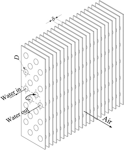
The tests were carried out with atmospheric air flowing through the fin passages of the heat exchanger and water flowing inside the tubes, under a wide range of operating conditions. The conditions were such that, for certain cases, condensation on the fins and tubes would occur. The nature of the air-side surface, i.e. whether dry, covered with condensed water droplets, or covered with a water film, was determined by direct observations and recorded. To visualize, photograph, and classify, the condensed water into film and dropwise conditions, a glass window was also included as part of the test facility; further details are in [3, 11], and in the original papers [8, 12].

Since McQuiston [8] was interested in predicting the air-side heat transfer, which was reported in terms of Colburn j-factors, high Reynolds-number turbulent flow on the water side was used to decouple the thermal resistances. For the dry surface conditions, the air-side heat transfer coefficients were determined using the log-mean temperature difference. A similar procedure was followed for determining the air-side heat transfer coefficients under condensing conditions by using the enthalpy difference as the driving potential.

The number of reported measurements was N = 327, of which 91 were classified as dry surface (N_dry), 117 as dropwise condensation (N_drop), and 119 as film condensation (N_film). The variables included: the inlet water temperature $T_{\mathrm{w}}^{\text{in}},$ the mass flow rate of air given in terms of Reynolds numbers based on the tube diameter Re_D, the dry-bulb and wet-bulb inlet temperatures of air $T_{\mathrm{a},\text{db}}^{\text{in}}$ and $T_{\mathrm{a},\text{wb}}^{\text{in}},$ the fin spacing δ, and the heat rate $\dot{Q}.$ The heat rate was determined from enthalpy balances between inlet and outlet of the external side of the heat exchanger. The corresponding ranges in the operating conditions [8], in SI system, are: $R{e}_{\mathrm{D}}\in [220,4270],T_{\mathrm{a},\text{db}}^{\text{in}}\in [22,31]$ °C, $T_{\mathrm{a},\text{wb}}^{\text{in}}\in [11,28]$ °C, $T_{\mathrm{w}}^{\text{in}}\in [1,72]$ °C, whereas the five values of the fin spacing are: $\delta =\{1.81,$ 2.11, 2.54, 3.18, $6.35\}$ mm. As a result, the heat rates are given in the range $\dot{Q}\in [205,4905]$ W.

For the prediction of the heat exchanger performance, the heat rate is a function of the inlet temperatures, the air-side mass flow rate and the fin spacing; i.e., $\dot{Q}=\dot{Q}(T_{\mathrm{w}}^{\text{in}},R{e}_{\mathrm{D}},T_{\mathrm{a},\text{db}}^{\text{in}},T_{\mathrm{a},\text{wb}}^{\text{in}},\delta ),$ which corresponds to a smooth manifold in a six-dimensional parameter space. For purposes of this study, it is possible to visualize the structure of the data by passing a set of planes through the hyper-surface, and Figure 2 illustrates a collection of plane-cuts of this manifold being arranged in matrix form. In the figure, for example, the top set of graphs provides information on the Reynolds number with respect to the variables $T_{\mathrm{a},\text{db}}^{\text{in}},T_{\mathrm{a},\text{wb}}^{\text{in}},T_{\mathrm{w}}^{\text{in}},$ δ, and $\dot{Q},$ respectively, whereas the bottom set shows the relationship between $\dot{Q}$ and the other five variables involved. Although only partial information is obtained in this way, it gives an idea of the interplay among the variables and the possible groups in which they could be classified.

Figure 2. Data representation through cut-planes.

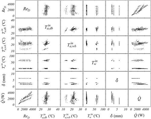
From inspection of the planes showing $T_{\mathrm{w}}^{\text{in}}$ as a function of the other variables, for instance, we can see that there are two well-formed groups, one of which – as will be shown in a later section – actually conforms to the data classified by McQuiston [8] as dry surface; the second group corresponds to data for humid conditions. On the other hand, for the set of planes that present δ as function of the other variables, the number of groups are five, matching the five values of the fin spacing. Finally, by observing the plane $\dot{Q}$ vs. Re_D, it can be noticed that the data are clustered in two groups, with a third one starting to appear at high Re_D. The disparity in the number of groups displayed in the different planes, illustrates the complexity of the identification process.

3. Classification by Gaussian mixtures clustering

3.1. Background

CA, discussed in detail in the texts by Everitt et al. [13] and Abonyi and Feil [14], is also known as clustering or numerical taxonomy. It is a soft computing (SC) methodology that classifies data into groups (or clusters), such that elements drawn from the same group are as similar to each other as possible, while those assigned to different groups are dissimilar. In contrast to the ANN supervised classification by learning processes, CA is often described as unsupervised pattern classification since the clusters are obtained solely from the data under the hypothesis that such data contain enough information inherent to the phenomenon of interest so that the parameters that characterize it can be established.

The application of CA has increased substantially in recent years in a variety of disciplines like geophysics [15], management [16], medicine [17], manufacturing [18], thermodynamics [19], multiphase flows [20, 21], and astronomy [22], among others, where the common thread is some kind of classification or feature extraction from experimental data. Though several techniques in CA have been developed, and excellent reviews are available [23, 24], this section concentrates on the Gaussian mixtures clustering (GMC) technique.

3.2. Description

Gaussian mixtures are frequently used to classify data into groups when the relationships among the data points are unknown. A main advantage offered by the method is the possibility of finding the number of groups as part of the solution. Its applications include structural damage detection [25], discrimination of single bacterial cells [26], identification of the circulatory regimes in the atmosphere [27], signal and image processing [28], and monitoring of chemical processes [29], among others. A clustering technique based on Gaussian mixtures assumes that the data can be grouped into a number of K clusters (c_i, for $i=1,\dots ,K$), each described by a multivariate Gaussian probability density distribution. Once the number of groups is known, the geometrical features (or structures) of such collections and the corresponding data classification are determined on the basis of a maximum likelihood (ML) criterion. Excellent descriptions of the technique, along with its mathematical background, are provided in several monographs [13, 30, 31]. The following is a brief account of the method.

Given a set of N experimental data, $\mathbf{X}=\{{\mathbf{x}}_1,{\mathbf{x}}_2,\dots ,{\mathbf{x}}_N\}\subset {\mathcal{R}}^q,$ the probability distribution of each q-dimensional measurement, ${\mathbf{x}}_j,$ may be described by a linear combination of K mixture components (1) $$p({\mathbf{x}}_j|\mathbf{\Psi })=\sum _{i=1}^{K}p({\mathbf{x}}_j|c_i,{\mathit{\theta }}_i)p(c_i),\mathrm{\hspace{1em}}\mathrm{\hspace{1em}}j=1,\dots ,N,$$(1) where $p(c_i)$ is the prior probability (also known as weight or mixing proportion) of group c_i occurring in the sample data; ${\sum }_{i=1}^{K}p(c_i)=1,$ and $p({\mathbf{x}}_j|c_i,{\mathit{\theta }}_i)$ is the conditional probability of ${\mathbf{x}}_j$ belonging to cluster c_i, being this modeled by a cluster-specific multivariate Gaussian density function (2) $$p({\mathbf{x}}_j|c_i,{\mathit{\theta }}_i)=\frac{1}{{(2\pi )}^{q/2}|{\Sigma }_i{|}^{1/2}}\text{exp}\hspace{0.17em}\left[-\frac{1}{2}{({\mathbf{x}}_j-{\mu }_i)}^T{\Sigma }_i^{-1}({\mathbf{x}}_j-{\mu }_i)\right].$$(2)

The parameters ${\mathit{\theta }}_i=\{{\mu }_i,{\Sigma }_i\}$ correspond to the $(q\times 1)$ vector of mean values μ_i, and the $(q\times q)$ covariance matrix Σ_i, which characterize the shape of each component density, and $\mathbf{\Psi }=\{(p(c_i),{\mathit{\theta }}_i): i=1,\dots ,K\}$ denotes the set of parameters of the entire mixture model.

The unknowns in Eqs. (1)(1) $$p({\mathbf{x}}_j|\mathbf{\Psi })=\sum _{i=1}^{K}p({\mathbf{x}}_j|c_i,{\mathit{\theta }}_i)p(c_i),\mathrm{\hspace{1em}}\mathrm{\hspace{1em}}j=1,\dots ,N,$$(1) and (2)(2) $$p({\mathbf{x}}_j|c_i,{\mathit{\theta }}_i)=\frac{1}{{(2\pi )}^{q/2}|{\Sigma }_i{|}^{1/2}}\text{exp}\hspace{0.17em}\left[-\frac{1}{2}{({\mathbf{x}}_j-{\mu }_i)}^T{\Sigma }_i^{-1}({\mathbf{x}}_j-{\mu }_i)\right].$$(2) are the number of clusters K, the parameters of the Gaussian distributions ${\mathit{\theta }}_i$ or $\{{\mathit{\theta }}_1,\dots ,{\mathit{\theta }}_K\}=\left\{\right\{{\mu }_1,{\Sigma }_1\},\dots ,\{{\mu }_K,{\Sigma }_K\left\}\right\},$ and the mixing proportions $p(c_i)$ or $\{p(c_1),\dots ,p(c_K)\},$ all of which can be computed from the data. A number of methods has been proposed to estimate the model parameters $\mathbf{\Psi },$ for a prescribed K, and the set of N observations, based on the well-known ML estimation approach. The ML methodology considers the best parameter estimate as that which maximizes the probability of generating the N observations, being this described by the joint density function in logarithm form as $L(\mathbf{X},\mathbf{\Psi })={\sum }_{j=1}^N\hspace{0.17em}\text{log}\hspace{0.17em}p({\mathbf{x}}_j|\mathbf{\Psi }).$ The result is a ML estimate of the vector $\mathbf{\Psi }=\left\{\right\{p(c_1),{\mathit{\theta }}_1\},\dots ,\{p(c_K),{\mathit{\theta }}_K\left\}\right\};$ i.e., $\widehat{\mathbf{\Psi }},$ as (3) $$\widehat{\mathbf{\Psi }}=\left\{(\widehat{p}(c_i),{\widehat{\mathit{\theta }}}_i): i=1,\dots ,K\right\}=\arg \underset{{}_{\stackrel{\mathbf{\Psi }}{}}}{\max }\sum _{j=1}^N\hspace{0.17em}\text{log}\hspace{0.17em}\left(\sum _{i=1}^{K}p({\mathbf{x}}_j|c_i,{\mathit{\theta }}_i)p(c_i)\right),$$(3) where ${\widehat{\mathit{\theta }}}_i=\{{\widehat{\mu }}_i,{\widehat{\Sigma }}_i\},$ and the symbol ‘  $\stackrel{\hspace{0.17em}}{}$ ’ denotes the final estimates of the corresponding quantities. Due to the fact that in most cases solutions of Eq. (3)(3) $$\widehat{\mathbf{\Psi }}=\left\{(\widehat{p}(c_i),{\widehat{\mathit{\theta }}}_i): i=1,\dots ,K\right\}=\arg \underset{{}_{\stackrel{\mathbf{\Psi }}{}}}{\max }\sum _{j=1}^N\hspace{0.17em}\text{log}\hspace{0.17em}\left(\sum _{i=1}^{K}p({\mathbf{x}}_j|c_i,{\mathit{\theta }}_i)p(c_i)\right),$$(3) cannot be obtained analytically, the usual approach is to solve it via numerical approximation with the well-known expectation-maximization (EM) algorithm [32], which iteratively performs two steps: an expectation step (e-step) of the complete data log-likelihood, followed by a maximization step (m-step) to update the parameter set that increases the value of the log-likelihood function (see Eq. (3)(3) $$\widehat{\mathbf{\Psi }}=\left\{(\widehat{p}(c_i),{\widehat{\mathit{\theta }}}_i): i=1,\dots ,K\right\}=\arg \underset{{}_{\stackrel{\mathbf{\Psi }}{}}}{\max }\sum _{j=1}^N\hspace{0.17em}\text{log}\hspace{0.17em}\left(\sum _{i=1}^{K}p({\mathbf{x}}_j|c_i,{\mathit{\theta }}_i)p(c_i)\right),$$(3) ), until a convergence criterion is satisfied.

The unknown number of clusters K, necessary for the data classification, can be estimated based on the minimum description length (MDL) criterion [33] (although several other criteria are available in the literature [24, 34, 35]). The MDL is a penalized function of the negative logarithm of the ML, i.e., (4) $$\text{MDL}(K,\mathbf{\Psi })=-\sum _{j=1}^N\hspace{0.17em}\text{log}\hspace{0.17em}\left(\sum _{i=1}^{K}p({\mathbf{x}}_j|c_i,{\mathit{\theta }}_i)p(c_i)\right)+\frac{1}{2}Kq\hspace{0.17em}\text{log}\hspace{0.17em}(Nq),$$(4) that provides a tradeoff between the data representation and the model complexity. Minimization of Eq. (4)(4) $$\text{MDL}(K,\mathbf{\Psi })=-\sum _{j=1}^N\hspace{0.17em}\text{log}\hspace{0.17em}\left(\sum _{i=1}^{K}p({\mathbf{x}}_j|c_i,{\mathit{\theta }}_i)p(c_i)\right)+\frac{1}{2}Kq\hspace{0.17em}\text{log}\hspace{0.17em}(Nq),$$(4) with respect to K gives the number of clusters that enables a good description of the data by the simplest Gaussian-mixtures model. The GMC methodology used in this work to determine $\mathbf{\Psi }$ and K is that of Chen et al. [36], who used the EM algorithm along with the MDL criterion as objective function. In their approach, the minimization starts with a large number of groups that are sequentially merged, two at a time, based on their inter-cluster distances. Additional details about the algorithm are in [36], and the references therein.

After K and $\widehat{\mathbf{\Psi }}$ are calculated, it is now possible to assign datum ${\mathbf{x}}_j$ to group c_i according to its maximum posterior probability, i.e., the probability that data point ${\mathbf{x}}_j$ belongs to the group c_i. The criterion is (5) $$\widehat{p}(c_i)p({\mathbf{x}}_j|c_i,{\widehat{\mathit{\theta }}}_i)>\widehat{p}(c_k)p({\mathbf{x}}_j|c_k,{\widehat{\mathit{\theta }}}_k),\hspace{1em}\text{for}\mathrm{ }\text{all}\hspace{1em}i\ne k;\hspace{1em}i,k=1,\dots ,K.$$(5)

3.3. Procedure

The steps of the GMC algorithm [36], used in this investigation, are as follows.

1. Initialization of parameters: The number of groups and the parameter set are initialized to K = K₀ (K₀ is a large number), and ${\mathbf{\Psi }}^{(0)}=\{(p^{(0)}(c_i),{\mathit{\theta }}_i^{(0)}): i=1,\dots ,K\},$ where ${\mathit{\theta }}_i^{(0)}=\{{\mu }_i^{(0)},{\Sigma }_i^{(0)}\},$ and the superscript shows the iteration number (i.e., n = 0), necessary during the EM calculation.

2. Calculation and updating of parameters: The EM algorithm is applied iteratively until the change in the log-likelihood function (see Eq. (3)(3) $$\widehat{\mathbf{\Psi }}=\left\{(\widehat{p}(c_i),{\widehat{\mathit{\theta }}}_i): i=1,\dots ,K\right\}=\arg \underset{{}_{\stackrel{\mathbf{\Psi }}{}}}{\max }\sum _{j=1}^N\hspace{0.17em}\text{log}\hspace{0.17em}\left(\sum _{i=1}^{K}p({\mathbf{x}}_j|c_i,{\mathit{\theta }}_i)p(c_i)\right),$$(3) ), is less than a specified tolerance. During the e-step, on the n-th iteration, the expectation of the complete data log-likelihood is computed. During the m-step, on the $(n+1)$-th iteration, the new values of the parameters for the Gaussian distributions and mixing proportions $\{p^{(n+1)}(c_i),{\mathit{\theta }}_i^{(n+1)}\},$ with ${\mathit{\theta }}_i^{(n+1)}=\{{\mu }_i^{(n+1)},{\Sigma }_i^{(n+1)}\},$ are determined. Once convergence of the EM method is achieved, for a given number of clusters K, the final estimates of the parameters are $\widehat{\mathbf{\Psi }}\equiv {\widehat{\mathbf{\Psi }}}_K=\{\widehat{p}(c_i),{\widehat{\mathit{\theta }}}_i\}=\{\widehat{p}(c_i),{\widehat{\mu }}_i,{\widehat{\Sigma }}_i\},$ for $i=1,\dots ,K.$

3. Evaluation of MDL and cluster consolidation: Using the estimated parameter set $\widehat{\mathbf{\Psi }},$ from the EM procedure, the objective function $\text{MDL}(K,\widehat{\mathbf{\Psi }}),$ i.e. Eq. (4)(4) $$\text{MDL}(K,\mathbf{\Psi })=-\sum _{j=1}^N\hspace{0.17em}\text{log}\hspace{0.17em}\left(\sum _{i=1}^{K}p({\mathbf{x}}_j|c_i,{\mathit{\theta }}_i)p(c_i)\right)+\frac{1}{2}Kq\hspace{0.17em}\text{log}\hspace{0.17em}(Nq),$$(4) , is computed first, and the information is stored for further analysis. Then, the two most similar groups (based on inter-cluster distance), are merged into one, and their parameters combined [36], thus reducing the number of groups to $(K-1).$

Steps 2 and 3 are repeated until the number of groups (Gaussian distributions) are reduced to one (K = 1), and the value of its corresponding MDL function has been computed. The final number of groups (clusters) $K\equiv \widehat{K},$ and the corresponding parameters $\widehat{\mathbf{\Psi }}\equiv {\widehat{\mathbf{\Psi }}}_{\widehat{K}}=\{\widehat{p}(c_i),{\widehat{\mathit{\theta }}}_i\}=\{\widehat{p}(c_i),{\widehat{\mu }}_i,{\widehat{\Sigma }}_i\},$ for $i=1,\dots ,\widehat{K},$ which provide the minimum value of $\text{MDL}(K,\widehat{\mathbf{\Psi }}),$ are selected as the optimum set.

4. Results and analysis from GMC classification

We now apply the GMC technique described in the previous section to the N = 327 heat exchanger experimental measurements of McQuiston [8], in order to first determine the number of operating regimes and then to classify the data into those regions. For the iterative process described in the previous section, the initial number of groups is $K_0=20,$ with the prior probabilities being initialized uniformly as $p^{(0)}(c_i)=1/K_0;$ the vector ${\mu }_i^{(0)},$ is randomly assigned values from the data ${\mathbf{x}}_j,$ and the initial covariance matrix is ${\Sigma }_i^{(0)}=(1/N){\sum }_{j=1}^N{\mathbf{x}}_j{\mathbf{x}}_j^T,$ forming the starting parameter set, ${\mathbf{\Psi }}^{(0)}=\{(p^{(0)}(c_i),{\mathit{\theta }}_i^{(0)}): i=1,\dots ,K_0\},$ for the Gaussian components.

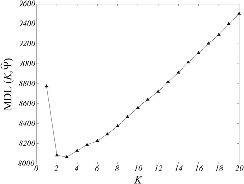
The corresponding results for the estimated number of groups (Gaussian mixtures), $K\equiv \widehat{K},$ are shown in Figure 3. The figure illustrates the evolution in the values of the objective function $\text{MDL}(K,\mathbf{\Psi }),$ with the number of clusters K, as the optimization proceeds. Starting with $K=K_0=20,$ and going down to $=1,$ it is possible to observe that the values of the MDL function first decrease monotonically from 9,510 to the minimum value of 8,055 when K = 3, then increasing to reach $\text{MDL}=8800$ at K = 1. Convergence of the algorithm to the minimum value of the MDL function at $K\equiv \widehat{K}=3$ clusters, concurs with the possible physical phenomena; i.e., dry-surface, dropwise-, and film-condensation (as determined visually [8]), taking place during the operation of the device.

Figure 3. Objective function $\text{MDL}(K,\widehat{\mathbf{\Psi }})$ vs. number of groups K. Optimum value of MDL occurs at $K\equiv \widehat{K}=3.$

The classification results are shown quantitatively in Table 1, in terms of the percentage of datasets of all three surface conditions that were allocated to a particular group I, II, or III. From the table, it can be observed that the GMC results and McQuiston [8] visual analysis agree completely in the dry-surface data, which were all assigned by the algorithm to group I. However, the agreement in the allocation of the data corresponding to humid conditions into groups II and III is less crisp, as each of these two groups contain data with a strong overlap between the different types of condensation. From the 117 datasets visually classified as drop condensation, only 35.89% were algorithmically allocated into group II, whereas the rest (64.11%) were placed in group III. Similarly, 25.21% of the film condensation data (N_film = 119), were clustered into group II, while 74.79% in group III. The actual numbers of data allocated into groups I, II, and II are, respectively, M_I = 91, M_II = 72, and M_III = 164.

Table 1. Percentage of data sets of different surface conditions classified into different groups by GMC methodology.

Surface/Group	I	II	III
Dry surface	100%	0	0
Drop condensation	0	35.89%	64.11%
Film condensation	0	25.21%	74.79%

Qualitative comparison between the algorithmic and visual classifications is shown in Figures 4–7, on a number of cut-planes of the hyper-surface $\dot{Q}=\dot{Q}(T_{\mathrm{w}}^{\text{in}},R{e}_{\mathrm{D}},T_{\mathrm{a},\text{db}}^{\text{in}},T_{\mathrm{a},\text{wb}}^{\text{in}},\delta ),$ with Figures 4a–7a illustrating the GMC results and Figures 4b–7b the visual descriptions. From Figures 4 and 5, for example, which display the planes Re_D vs. $T_{\mathrm{w}}^{\text{in}}$ and $\dot{Q}$ vs. $T_{\mathrm{w}}^{\text{in}},$ respectively, it can be seen that not only a clear separation between the sets of data corresponding to high- and low-values of inlet water temperature $T_{\mathrm{w}}^{\text{in}}$ exists but also that the algorithmic allocation of the data for high inlet-water-temperature values (i.e., $T_{\mathrm{w}}^{\text{in}}>{55}^{°}$ C), placed into group I, completely agrees with the visual procedure for the set of dry-surface conditions, confirming the results of Table 1. However, for low values of inlet water-temperature (i.e., $T_{\mathrm{w}}^{\text{in}}<{10}^{°}$ C), correlating with wet-surface conditions, there is a clear difference in both quantity and distribution of the experimental measurements between those grouped by the GMC technique and the data visually clustered. For instance, though the wet-surface data is allocated into two groups (groups II and III, as observed in the table), and there is a significant overlap in the data between the different types of condensation and both clusters; from the figures, it is evident that a number of datasets allocated by the GMC do not match the specific drop or film surface-condition data. However, while there is not a clear pattern from either type of classification in Figure 4, by looking at the plane $\dot{Q}$ vs. $T_{\mathrm{w}}^{\text{in}},$ in Figure 5, some order exists in the algorithmic results, which show that group II contains data in mostly lower values of the heat rate while group III has data in the higher $\dot{Q}$-values. This is drastically different from the visual allocation which displays drop- and film-condensation data in the entire $\dot{Q}$-range.

Figure 4. Heat exchanger data classification. Plane Re_D vs. $T_{\mathrm{w}}^{\text{in}}.$ (a) Algorithmically via GMC; (b) Visually by [8].

Figure 5. Heat exchanger data classification. Plane $\dot{Q}$ vs. $T_{\mathrm{w}}^{\text{in}}.$ (a) Algorithmically via GMC; (b) Visually by [8].

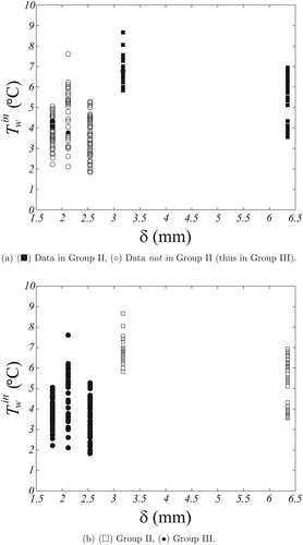
Figure 6. Heat exchanger data classification. Plane $T_{\mathrm{w}}^{\text{in}}$ vs. δ. (a) Algorithmically via GMC; (b) Visually by [8].

Figure 7. Heat exchanger data classification. Plane $\dot{Q}$ vs. Re_D. (a) Algorithmically via GMC; (b) Visually by [8].

In Figure 6, which depicts the plane $T_{\mathrm{w}}^{\text{in}}$ vs. δ, it is possible to verify that both the GMC algorithm and the visual procedure agree entirely in the dry-surface data allocation to group I (occurring at high values of $T_{\mathrm{w}}^{\text{in}},$ and for all five values of fin spacing). However, by looking at Figure 6a, it can be seen that the set of data corresponding to wet-surface conditions is also well separated by the GMC technique with respect to fin spacing; for small values of δ, the allocation of the data is into group III, whereas for large δ-values the data are placed into group II. Again, this is drastically distinct from the visual allocation in Figure 6b, which indicates that both film and drop condensation data occur, without a clear pattern, for the entire set of values of fin spacing.

Finally, the information shown in Figure 7, on the $\dot{Q}$ vs. Re_D plane, illustrates that not only the dry-surface and group I data correlate but also – in agreement with the results of Figure 5 – there is a pattern in the algorithmic data-classification for the wet-surface conditions, as it can be seen that the GMC method is able to clearly separate the data onto groups II and III, while it is difficult to distinguish the trend in the data classified by the visual procedure (see Figure 7b). In fact, from Figure 7a, it is possible to observe that for a fixed value of Re_D, the values of $\dot{Q}$ from group II are always lower than those of the data in group III. In this case, with the heat rate $\dot{Q}$ as the discriminant variable, the physical phenomena involved in the transfer of heat in these thermal systems imply that higher values of it resemble the case of dropwise condensation, whereas for the same operating conditions (e.g., same Re_D-values), lower $\dot{Q}$-values match the case of film condensation [1, 37].

It is to note that the discrepancies between the algorithmic and visual classifications of the condensing (wet-surface) operating conditions of the heat exchanger data, may rise the question as to which classification is correct. This question is addressed in the next sections using a methodology based on ANNs, which was developed as part of the present investigation.

5. Classification by ANNs

To assess the correctness of the data classification by the Gaussian-mixtures-based clustering algorithm, the experimental data are now classified with a novel procedure based on the popular ANN technique. Neural networks learn from external experience in a supervised manner and have been successfully applied to a variety of disciplines, such as: philosophy, psychology, economics, science, and engineering, among others, where some kind of pattern recognition process was necessary. Comprehensive information about the subject is available in introductory texts, among which those of Schalkoff [38] and Haykin [39] cover its history, its mathematical background and implementation procedures. A brief description of the technique is given next.

5.1. Background

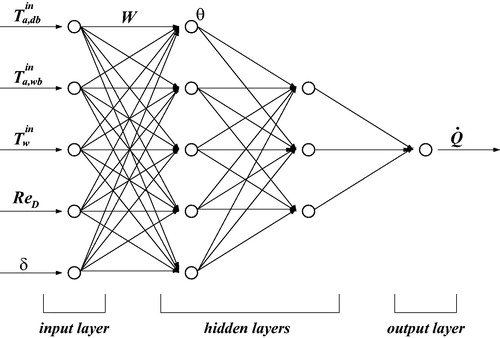
Although various types of ANNs exist, the fully connected feedforward configuration has become the most popular in thermal engineering applications [2, 3], and it is the type of network used here to develop the classification methodology. A fully connected network consists of a large number of interconnected processing units that are organized in layers. The first and last layers are the input and output layers, while the remaining are the hidden layers. The nodes in each layer are connected to those of the following layer by means of synaptic weights. The configuration of the ANN is set by choosing the number of hidden layers and the number of nodes in each of these; the number of nodes in the input and output layers are selected based on the physical variables of the specific problem under analysis. Nodes in the hidden layers perform nonlinear input-output mappings by means of sigmoid activation functions.

A typical feedforward architecture for the problem at hand is illustrated schematically in Figure 8. This neural network – which is similar to that used to predict the performance of the same set of condensing heat exchangers [11] – consists of four layers: the input layer at the left containing five nodes, two hidden layers with five and three nodes, respectively, and the output layer at the right having a single node. Since the heat rate is a function of inlet temperatures, flow rates and the geometry, then the input variables of this 5-5-3-1 ANN configuration are: Re_D, $T_{\mathrm{w}}^{\text{in}},T_{\mathrm{a},\text{db}}^{\text{in}},T_{\mathrm{a},\text{wb}}^{\text{in}},$ and δ, whereas the output variable is $\dot{Q}.$ All variables are usually normalized within the typical $[0.15,0.85]$ range.

Figure 8. A 5-5-3-1 ANN model of the heat exchanger system.

The training process for the neural network is carried out by comparing its output to the given data. During the feedforward stage, the set of input data is supplied to the input nodes and the information is transferred forward through the network to the nodes in the output layer. The actual output is then compared with the target, and the weights and biases are repeatedly adjusted by the backpropagation algorithm [40] until the error between actual and target outputs is small. Feedforward followed by backpropagation of all the data comprises a training cycle. Further details are in [3] and the references therein. It is to note that in this study, for all the cases described next, initially 70% of the data were used for training whereas the other 30% are taken aside for testing purposes. However, following the findings of Pacheco-Vega et al. [11, 41], in each case the final ANN model used for the data classification procedure was built with 100% of the data available, since it furnishes the best possible model over the widest parameter range.

5.2. Description of classification methodology

The ANN classification methodology established as part of this study is grounded on the idea that given two sets of data, e.g., one for training and the other for testing, if these datasets have common patterns (structures), the ANN model built with the training set will provide a small prediction error on the testing set; otherwise, the prediction error will be large. A similar concept was used by Pacheco-Vega et al. [41], to develop an estimation method of the reliability of ANN predictions under limited amount of data, based on a variant of the cross-validation statistical tool. For the problem at hand, the prediction error from a trained ANN can be quantified in terms of the percentage difference between the target values and the ANN predictions of the heat rate $\dot{Q},$ as (6) $$E_{\mathrm{p},j}=\left|\frac{{\dot{Q}}_j^{e,t}-{\dot{Q}}_j^{p,\text{ANN}}}{{\dot{Q}}_j^{e,t}}\right|\times 100,\mathrm{\hspace{1em}}\mathrm{\hspace{1em}}j=1,\dots ,N,$$(6) where ${\dot{Q}}_j^{e,t}$ and ${\dot{Q}}_j^{p,\text{ANN}},$ for datum j, are the target values and the ANN predictions, respectively, and N is the total number of experimental data.

Distinguishing data that are part of a specific group (or cluster), from those that do not belong to that particular set, is carried out by comparing the prediction error E_p in Eq. (6)(6) $$E_{\mathrm{p},j}=\left|\frac{{\dot{Q}}_j^{e,t}-{\dot{Q}}_j^{p,\text{ANN}}}{{\dot{Q}}_j^{e,t}}\right|\times 100,\mathrm{\hspace{1em}}\mathrm{\hspace{1em}}j=1,\dots ,N,$$(6) , to the lower-bound of the maximum error obtained during the training process of the ANN, namely E_T, as follows:

• If $E_{\mathrm{p}}\le E_{\mathrm{T}},$ then testing and training data points have common structures and, therefore, they belong to the same group/set.

• If E_p > E_T, then testing and training data points do not have common patterns and, therefore, they do not belong to the same group/set.

6. Results and analysis from ANN classification

In order assess the classification of the GMC technique, we now apply the ANN allocation methodology to the N = 327 datasets of McQuiston [8], as classified by the visual process; i.e., N_dry = 91, N_drop = 117, and N_film = 119, and the corresponding GMC allocation into three groups, with M_I = 91, M_II = 72, and M_III = 164 datasets, according to the following procedure.

1. We first train three different ANNs, all having the same 5-5-3-1 configuration mentioned above, but each with a different dataset from reference [8]. For example, ANN₁ is trained with only the N_dry = 91 dry surface data, whereas ANN₂ is trained with the N_drop = 117 data corresponding to dropwise condensation, and ANN₃ with the N_film = 119 film-condensation data. The training errors $E_{\mathrm{T}}^1,E_{\mathrm{T}}^2,$ and $E_{\mathrm{T}}^3,$ are also recorded.

2. Then, using ANN₁ and the M_I = 91 data in group I, the error $E_{\mathrm{p}}^{1,\mathrm{I}},$ is computed and compared to the corresponding training error $E_{\mathrm{T}}^1,$ and the data are classified according to the aforementioned procedure into data that either belong or do not belong to the training set and to group I (data from groups II and III are also tested for completeness). Similar procedures are performed with ANN₂ and the M_II = 72 data from group II (with the corresponding error $E_{\mathrm{p}}^{2,\text{II}}$), and ANN₃ with the M_III = 164 datasets of group III, and prediction error $E_{\mathrm{p}}^{3,\text{III}}.$ It is to be noted that other testing combinations (e.g., ANN₂ with the M_III datasets, and/or ANN₃ with the M_II-data), which lead to equivalent allocation results, are also possible.

The classification results from the ANN-based methodology are shown quantitatively, as agreement in percentage between the ANN allocation and the visual procedure of McQuiston [8], in Table 2. From the table, it can be seen that – as it was the case with the results from the GMC algorithm – the ANN distribution method completely agrees with the visual procedure for the dry-surface data, which were all found to belong to group I. However, the agreement in the allocation of the data corresponding to the humid conditions (drop and film condensation) into groups II and III is not as sharp, since data for drop condensation were assigned by the ANN technique into groups II (34.19%) and III (65.81%), with a similar outcome for the data corresponding to film condensation into groups II (21.85%) and III (78.15%). On the other hand, when comparing these results to the classification provided by the GMC methodology in Table 1, it can be observed that the two algorithmic allocations are in almost perfect agreement. The two tables indicate that the complete set of data in group I is that of dry-surface conditions, whereas there is a difference of only 1.7% (two data points) between the distribution provided by the ANN methodology and that of the clustering technique for the case of dropwise condensation onto groups II and III, and a difference of 3.36% (four data points), between the two methods for the film-condensation data onto groups II and III.

Table 2. Percentage of data sets of different surface conditions classified into different groups by ANN methodology.

Surface/Group	I	II	III
Dry surface	100%	0	0
Drop condensation	0	34.19%	65.81%
Film condensation	0	21.85%	78.15%

Qualitatively, Figures 9 and 10 show the corresponding results for wet-surface conditions only (the dry-surface data have been excluded for clarity purposes), using the $\dot{Q}$ vs. Re_D and $T_{\mathrm{w}}^{\text{in}}$ vs. δ planes, respectively. In both figures, the ANN allocations are illustrated in Figures 9a and 10a, whereas the GMC placements are shown in Figures 9b and 10b. From the figures, it can be clearly seen that both algorithmic classification methodologies are extremely close in their results – number and the data in each group – with only few discrepancies between them; in fact, the number of mismatches is only of six in 236 datasets, confirming the quantitative information of Tables 1 and 2. These results demonstrate remarkable accuracy from both classification methodologies in the allocation of the data into the different surface conditions from the heat exchanger operation, and show that either technique could be used to algorithmically separate the corresponding experimental measurements. The advantage of the GMC technique, over the ANN-based method, is in the fact that the number of groups in which the data can be separated is obtained from the process in the earlier instead of having to know it a priori for the latter. Finally, the disagreement of the two algorithms with the visual classification is indicative of the complexity of the phenomenon involved in the transfer of heat in the thermal system and the necessity of an alternative classification approach to visual procedures.

Figure 9. Heat exchanger data classification for wet-surface conditions. Plane $\dot{Q}$ vs. Re_D. (a) Algorithmically via ANN methodology; (b) Algorithmically via GMC methodology.

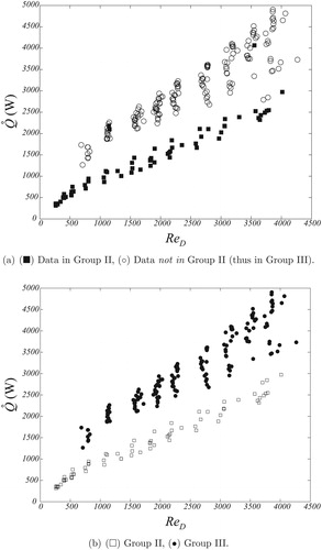
Figure 10. Heat exchanger data classification for wet-surface conditions. Plane $T_{\mathrm{w}}^{\text{in}}$ vs. δ. (a) Algorithmically via ANN methodology; (b) Algorithmically via GMC methodology.

7. Concluding remarks

Heat exchangers are important in a number of applications, and their design, selection and control require accurate estimation of the performance. Predicting the system behavior, however, is not straightforward; the thermal design engineer typically resorts to using semi-empirical correlation models built from experimental measurements which, frequently, have to be classified into the appropriate physical conditions resulting from operation of the device. The effectiveness of the procedure depends on, among other factors, the reliability of the classification process, universally attained using visual techniques, and though visual data-allocation may be reliable for simple phenomena, the procedure may lead to large uncertainties in more complex cases. Thus, an alternative to reduce the uncertainty in the classification process – and increase the accuracy of correlations for predicting the behavior of heat exchangers – may be to algorithmically identify and characterize the information of the system.

In the present work, we have described a methodology able to extract the regimes of operation from condensing heat exchanger data. The methodology is grounded on a GMC algorithm to determine the number of groups directly from the data, and a ML decision rule to classify such data into these clusters. Results from its application to condensing heat exchanger data, visually classified as dry-surface, drop-, and film-condensation, show that the GMC-based methodology is able to accurately identify the data corresponding to each of the conditions in the system, as demonstrated by independent assessment using a novel procedure grounded on ANNs, which was also derived as part of this investigation. The ANN-based allocation method uses a typical feedforward architecture with the backpropagation error algorithm, along with a variant of the cross-validation approach, to find patterns in the data which enable their allocation into preestablished groups. Results from the ANN approach show remarkable agreement with the GMC technique confirming that an algorithmic classification is not only possible but also accurate in finding the different regimes of operation and classifying the data corresponding to each regime. This concept of an algorithmic approach to data classification represents an excellent alternative to typical visual-based procedures for the analysis of complex physical phenomena occurring in thermal and energy systems.

Nomenclature
ci	=	i-th group, cluster
D	=	tube outer diameter (mm)
E	=	classification error
ET	=	training error
Ep	=	percentage error in neural network predictions
K	=	total number of clusters, groups, mixture components
$L(\mathbf{X},\mathbf{\Psi })$	=	likelihood function
$M_{\mathrm{I}},M_{\text{II}},M_{\text{III}}$	=	number of data points in clusters I, II, and III
N	=	total number of experimental data sets
Ndry	=	number of data sets with dry surface
Ndrop	=	number of data sets with dropwise condensation
Nfilm	=	number of data sets with film condensation
p	=	probability
$p(c_i)$	=	prior probability (or weight) for cluster ci
$p({\mathbf{x}}_j|c_i,{\mathit{\theta }}_i)$	=	conditional probability of ${\mathbf{x}}_j$ in cluster ci
$\dot{Q}$	=	heat transfer rate between fluids (W)
ReD	=	air-side Reynolds number based on tube diameter
$T_{\mathrm{a},\text{db}}$	=	dry-bulb temperature of air (°C)
$T_{\mathrm{a},\text{wb}}$	=	wet-bulb temperature of air (°C)
Tw	=	temperature of water (°C)
X	=	vector of data sets
${\mathbf{x}}_j$	=	j-th data set in q-dimensional space
W	=	synaptic weight between nodes
Greek symbols	=
δ	=	fin spacing (mm)
θ	=	bias
${\mathit{\theta }}_i=\{{\mu }_i,{\sigma }_i\}$	=	parameter set for Gaussian distribution
μi	=	q-dimensional vector of mean-values
Σi	=	$(q\times q)$ covariance matrix
$\mathbf{\Psi }=\left\{p(c_i),{\mathit{\theta }}_i\right\}$	=	parameter set for entire Gaussian mixtures model
Subscripts and superscripts	=
ANN	=	artificial neural network
e	=	experimental value
in	=	inlet
n	=	iteration number
p	=	predicted value
T	=	transposed
t	=	target value
$\widehat{}$	=	final estimated value
0	=	initial state
Abbreviations	=
ANN	=	artificial neural network
CA	=	cluster analysis
EM	=	expectation-maximization
GMC	=	Gaussian mixtures clustering technique
GMM	=	Gaussian mixtures model
ML	=	maximum likelihood
MDL	=	minimum description length

Additional information

Funding

This work has been supported by the National Science Foundation with Award No. HRD-1547723.

References

- F. P. Incropera and D. P. DeWitt, Fundamentals of Heat and Mass Transfer. New York, NY, USA: Wiley, 2002.
- A. Pacheco-Vega, “Soft computing applications in thermal energy systems,” in Soft Computing in Green and Renewable Energy Systems, Studies in Fuzziness and Soft Computing, vol. 269, K. Gopalakrishnan, S. K. Khaitan, and S. Kalogirou, Eds. Berlin, Germany: Springer-Verlag, 2011, pp. 1–35.
- A. Pacheco-Vega, G. Diaz, M. Sen, and K. T. Yang, “Applications of artificial neural networks and genetic methods in thermal engineering,” in CRC Handbook of Thermal Engineering, chapter 4.27, 2nd ed., R. P. Chhabra, Ed. Boca Raton, FL, USA: CRC Press, 2017, pp. 1217–1269.
- A. Pacheco-Vega, M. Sen, and K. T. Yang, “Simultaneous determination of in- and over-tube heat transfer correlations in heat exchangers by global regression,” Int. J. Heat Mass Transfer, vol. 46, no. 6, pp. 1029–1040, 2003. DOI: 10.1016/S0017-9310(02)00365-4.
- A. Pacheco-Vega, M. Sen, and K. T. Yang, “Genetic-algorithm-based-predictions of fin-tube heat exchanger performance,” presented at the Eleventh International Heat Transfer Conference, vol. 6, R. L. McClain and J. S. Lee, Eds. New York, NY, USA: Taylor & Francis, August, 1998, pp. 137–142.
- W. Cai, A. Pacheco-Vega, M. Sen, and K. T. Yang, “Heat transfer correlations by symbolic regression,” Int. J. Heat Mass Transfer, vol. 49, no. 23–24, pp. 4352–4359, 2006. DOI: 10.1016/j.ijheatmasstransfer.2006.04.029.
- L. Cheng, G. Ribatski, and J. R. Thome, “Two-phase flow patterns and flow-pattern maps: Fundamentals and applications,” Appl. Mech. Rev., vol. 61, no. 5, pp. 050802, 2008. DOI: 10.1115/1.2955990.
- F. C. McQuiston, “Heat, mass and momentum transfer data for five plate-fin-tube heat transfer surfaces,” ASHRAE Trans., vol. 84, no. 1, pp. 266–293, 1978.
- F. C. McQuiston, “Correlation of heat, mass and momentum transport coefficients for plate-fin-tube heat transfer surfaces with staggered tubes,” ASHRAE Trans., vol. 84, no. 1, pp. 294–309, 1978.
- D. L. Gray and R. L. Webb, “Heat transfer and friction correlations for plate finned-tube heat exchangers having plain fins,” presented at the Eighth International Heat Transfer Conference, in C. L. Tien, V. P. Carey, and J. K. Ferrel, Eds., vol. 6, New York, NY, USA: Hemisphere 1986, pp. 2745–2750.
- A. Pacheco-Vega, G. Diaz, M. Sen, K. T. Yang, and R. L. McClain, “Heat rate predictions in humid air-water heat exchangers using correlations and neural networks,” ASME J. Heat Transfer, vol. 123, no. 2, pp. 348–354, 2001. DOI: 10.1115/1.1351167.
- F. C. McQuiston, “Heat, mass and momentum transfer in a parallel plate dehumidifying exchanger,” ASHRAE Trans., vol. 82, no. 2, pp. 87–106, 1976.
- B. S. Everitt, S. Landau, M. Leese, and D. Stahl, Cluster Analysis, 5th ed. Chichester, West Sussex, UK: Wiley, 2011.
- J. Abonyi and B. Feil, Cluster Analysis for Data Mining and System Identification, Berlin, Germany: Birkhăuser Verlag AG, 2007.
- H. Paasche and J. Tronicke, “Cooperative inversion of 2D geophysical data sets: A zonal approach based on fuzzy c-means cluster analysis,” Geophysics, vol. 72, no. 3, pp. A35–A39, 2007. DOI: 10.1190/1.2670341.
- D. J. Ketchen and C. L. Shook, “The application of cluster analysis in strategic management research: An analysis and critique,” Strateg. Manage. J., vol. 17, no. 6, pp. 441–458, 1996. DOI: 10.1002/(SICI)1097-0266(199606)17:6<441::AID-SMJ819>3.0.CO;2-G.
- W. J. Chen, M. L. Giger, U. Bick, and G. M. Newstead, “Automatic identification and classification of characteristic kinetic curves of breast lesions on DCE-MRI,” Med. Phys., vol. 33, no. 8, pp. 2878–2887, 2006. DOI: 10.1118/1.2210568.
- K. W. Johnson, P. M. Langdon, and M. F. Ashby, “Grouping materials and processes for the designer: An application of cluster analysis,” Mater. Des., vol. 23, no. 1, pp. 1–10, 2002. DOI: 10.1016/S0261-3069(01)00035-8.
- G. Avila and A. Pacheco-Vega, “Fuzzy C-means-based classification of thermodynamic-property data: A critical assessment,” Numer. Heat Transfer Part A, vol. 56, no. 11, pp. 880–896, 2009. DOI: 10.1080/10407780903466444.
- H. Caniere, B. Bauwens, C. T’Joen, and M. De Paepe, “Mapping of horizontal refrigerant two-phase flow patterns based on clustering of capacitive sensor signals,” Int. J. Heat Mass Transfer, vol. 53, no. 23–24, pp. 5298–5307, 2010. DOI: 10.1016/j.ijheatmasstransfer.2010.07.027.
- R. Amaya-Gomez, et al., “Probabilistic approach of a flow pattern map for horizontal, vertical, and inclined pipes,” Oil Gas Sci. Technol. – Rev. IFP Energies Nouvelles, vol. 74, pp. 67, 2019. (Article number: 67). DOI: 10.2516/ogst/2019034.
- M. Faúndez-Abans, M. I. Ormeno, and M. de Oliveira-Abans, “Classification of planetary nebulae by cluster analysis and artificial neural networks,” Astron. Astrophys. Suppl. Ser., vol. 116, no. 2, pp. 395–402, 1996. DOI: 10.1051/aas:1996122.
- A. K. Jain, M. N. Murty, and P. J. Flynn, “Data clustering: A review,” ACM Comput. Surv., vol. 31, no. 3, pp. 264–323, 1999. DOI: 10.1145/331499.331504.
- R. Xu and D. Wunsch, “Survey of clustering algorithms,” IEEE Trans Neural Netw., vol. 16, no. 3, pp. 645–678, 2005. DOI: 10.1109/TNN.2005.845141.
- K. K. Nair and A. S. Kiremidjian, “Time series based structural damage detection algorithm using Gaussian mixtures modeling,” J. Dynamic Syst. Meas. Control–Trans. ASME, vol. 129, no. 3, pp. 285–293, 2007. DOI: 10.1115/1.2718241.
- U. Schmid, P. Rösch, M. Krause, M. Harz, J. Popp, and K. Baumann, “Gaussian mixture discriminant analysis for the single-cell differentiation of bacteria using micro-Raman spectroscopy,” Chemometr. Intell. Lab. Syst., vol. 96, no. 2, pp. 159–171, 2009. DOI: 10.1016/j.chemolab.2009.01.008.
- B. Christiansen, “Atmospheric circulation regimes: Can cluster analysis provide the number?,” J. Climate, vol. 20, no. 10, pp. 2229–2250, 2007. DOI: 10.1175/JCLI4107.1.
- M. J. Carlotto, “A cluster-based approach for detecting man-made objects and changes in imagery,” IEEE Trans. Geosci. Remote Sens., vol. 43, no. 2, pp. 374–387, 2005. DOI: 10.1109/TGRS.2004.841481.
- J. Yu and S. J. Qin, “Multimode process monitoring with Bayesian inference-based finite Gaussian mixture models,” AIChE J., vol. 54, no. 7, pp. 1811–1829, 2008. DOI: 10.1002/aic.11515.
- A. Webb, Statistical Pattern Recognition. New York, USA: Wiley, 2002.
- T. Mitchell, Machine Learning. New York, NY: McGraw-Hill, 1997.
- A. P. Dempster, N. M. Laird, and D. B. Rubin, “Maximum likelihood from incomplete data via EM algorithm,” J. R. Stat. Soc. B, vol. 39, no. 1, pp. 1–38, 1977. DOI: 10.1111/j.2517-6161.1977.tb01600.x.
- J. Rissanen, “A universal prior for integers and estimation by minimum description length,” Ann. Statist., vol. 11, no. 2, pp. 417–431, 1983.
- P. M. B. Vitányi and M. Li, “Minimum description length induction, Bayesianism, and Kolmogorov complexity,” IEEE trans. Inform. Theory, vol. 46, no. 2, pp. 446–464, 2000.
- A. K. Jain, “Data clustering: 50 years beyond K-means,” Pattern Recognit. Lett., vol. 31, no. 8, pp. 651–666, 2010. DOI: 10.1016/j.patrec.2009.09.011.
- S. Chen, C. A. Bouman, and M. J. Lowe, “Clustered components analysis for functional MRI,” IEEE Trans. Med. Imaging, vol. 23, no. 1, pp. 85–98, 2004. DOI: 10.1109/TMI.2003.819922.
- J. W. Rose, “Dropwise condensation theory and experiment: A review,” Proc. Inst. Mech. Eng. Part A: J. Power Energy, vol. 216, no. 2, pp. 115–128, 2002. DOI: 10.1243/09576500260049034.
- R. J. Schalkoff, Artificial Neural Networks. Boston, MA, USA: McGraw-Hill, 1997.
- S. Haykin, Neural Networks, a Comprehensive Foundation. Upper Saddle River, NJ, USA: Prentice-Hall, 1999.
- D. E. Rumelhart, G. E. Hinton, and R. J. Williams, “Learning internal representations by error propagation,” in Parallel Distributed Processing: Explorations in the Microstructure of Cognition, D. E. Rumelhart and J. L. McClellan, Eds. Cambridge, MA, USA: MIT Press, 1986, pp. 8.318–8.362.
- A. Pacheco-Vega, M. Sen, K. T. Yang, and R. L. McClain, “Neural network analysis of fin-tube refrigerating heat exchanger with limited experimental data,” Int. J. Heat Mass Transfer, vol. 44, no. 4, pp. 763–770, 2001. DOI: 10.1016/S0017-9310(00)00139-3.