Novel heat flux expansion formula for spacecraft solar radiation uncertainty analysis

Abstract

To address the challenges of spacecraft design involving over and under-designing, uncertainty thermal analysis offers a practical solution. This method typically requires extensive simulations under varying conditions, leading to high computational costs, primarily due to the complex ray tracing calculations for solar radiation external heat flux in different scenarios. This study introduces an solar radiation external heat flux expansion (EHFE) formula that simplifies these calculations. By applying ray tracing only once and using matrix operation for other conditions, it significantly reduces the need for complex calculations. Additionally, this approach effectively eliminates errors caused by the cut-off factor. An example with a specific spacecraft demonstrates that this new method, while enhancing computational efficiency, maintains the accuracy of traditional uncertainty-based calculations for solar radiation external heat flux.

Keywords:

• External heat flux expansion formula
• ray tracing
• solar radiation external heat flux
• spacecraft
• uncertainty thermal analysis

1. Introduction

As advancements in space technology persist and the demand for its applications grows, the robustness and reliability of spacecraft thermal control systems are subject to increasingly stringent requirements. The space environment poses numerous challenges in maintaining stable temperature conditions for spacecraft. Specifically, thermal analysis must address uncertainties stemming from various factors, including material properties, space environment conditions, solar radiation, Earth’s infrared and albedo radiation, heat transfer mechanisms, internal heat sources, temperature sensors, thermal modeling, and spacecraft attitude. The cumulative effect of these uncertainties can significantly influence the spacecraft’s structural temperature field, potentially leading to equipment damage and failure under certain circumstances [1, 2].

In conventional thermal design approaches, engineers frequently take into account worst-case scenarios to guarantee the spacecraft’s capacity to endure extreme conditions. This entails pinpointing the most demanding combination of environmental factors, such as maximal solar radiation, minimal or maximal albedo, and extreme temperatures, and subsequently designing the thermal control system to withstand these circumstances. Following the analysis, a predetermined design margin is implemented to address the uncertainty generated by the remaining parameters. These margins are derived from a statistical investigation of discrepancies between thermal model temperature predictions and in-flight measurements across a multitude of space missions [3].

Traditional approaches to the thermal design and verification of spacecraft do not address model uncertainty strictly upstream of the model. Instead, uncertainty is handled downstream of the model, and fixed design margins are applied directly to the model output. The work of Ishimoto and Bevans [4] and Howell [5] demonstrates that the primary objective of conducting uncertainty analysis is to devise an improved method for calculating these design margins. The central concept is that model uncertainty is rigorously considered prior to the model’s development and propagated through the model to the output, subsequently quantifying the uncertainty in the model output. Its advantage over traditional techniques lies in its capacity to provide design margins for specific cases, thereby reducing over-design and mitigating under-design issues.

By explicitly quantifying and accounting for uncertainties, uncertainty thermal analysis offers a more comprehensive understanding of the spacecraft’s thermal performance, facilitating better-informed design decisions and risk management. Incorporating probabilistic and sensitivity analysis enables the identification of critical parameters and their impacts, directing optimization efforts and prioritizing areas for enhancement. Additionally, uncertainty thermal analysis emphasizes model validation and refinement, resulting in more precise thermal predictions and efficient thermal control systems. In summary, uncertainty thermal analysis contributes to the development of more robust, reliable, and optimized spacecraft designs that more effectively account for the inherent variability within the space environment.

Currently, the Monte Carlo (MC) method is the main method that is used for uncertain thermal analysis calculations of spacecraft. However, Monte Carlo simulations can be computationally expensive, requiring a large number of runs to achieve statistically meaningful results. This can be time-consuming and resource-intensive, especially for complex thermal models. A great deal of research has been done to balance the accuracy as well as the speed of uncertainty thermal analysis algorithms. Thunnissen et al. [6] employed subset simulation for uncertainty transient thermal analysis during the cruise phase of a Mars spacecraft. The tail probability distribution function for the maximum temperature of crucial components was determined, showing good agreement with Monte Carlo (MC) results and significantly reduced computational effort. Gómez-San-Juan et al. [7] improved SEA and proposed a one-dimensional generalized statistical error analysis method. The input uncertainty variables of the method can be arbitrarily distributed. The nonlinear relationship between the node temperature and uncertainty variables is taken into account. It is comparable to the SEA in terms of the computation time and to the MC in terms of the accuracy. Xiong et al. [8] used a radial basis function neural network and an improved thinking evolutionary algorithm to approximate traditional spacecraft thermophysical models, effectively improving the analysis rate of uncertainty steady-state thermal analysis within the trained neural network. Kato et al. [9] utilized a simulator with Gaussian process regression and a minimum absolute shrinkage selection operator for satellite uncertainty thermal analysis, reducing the cost of uncertainty quantification. Similarly, the Kriging model [10–13], radial basis function [14], artificial neural network [15, 16], support vector regression [17], and response surface method [18] serve as approximate models that replace spacecraft thermal analysis models. Uncertainty thermal analysis is performed on the approximate model to improve the computational efficiency. However, the original thermal analysis model of the spacecraft still needs to be fully sampled and calculated several times to obtain an accurate approximate model. This can be challenging in high-dimensional or complex parameter spaces.

The above method improves the computational efficiency of uncertain thermal analysis from the viewpoint of mathematical methods. In this article, the original thermal analysis model of spacecraft is optimized to improve the computational efficiency of uncertainty thermal analysis. During the calculation of the original thermal analysis model of the spacecraft, the radiation model calculation and the thermal model calculation are the two main calculation steps to obtain the temperature field of the spacecraft. Gómez-San-Juan et al. [7] states that the time for the radiative model calculations is much longer than the time for the thermal model calculations. The radiative Monte Carlo ray tracing calculation is the most time-consuming task. Radiation Monte Carlo ray tracing calculations mainly include the complex processes of ray emission points, generation of emission directions, and determination of multiple intersections of the ray with the spacecraft. This involves tracking a large number of rays to simulate the radiative heat transfer between surfaces and is the most time-consuming task. The solar radiation external heat flux solution is an important part of the radiation model calculation. The need to calculate the solar radiation external heat flux several times using the Monte Carlo ray tracing algorithm is a main reason for the very large computational cost of uncertainty thermal analysis.

In the process of performing thermal analysis of uncertain spacecraft, random numbers are used to generate samples of the thermal property parameters for multiple operating conditions. The solutions of the solar radiation external heat flux for each working condition are independent of each other. Repeatedly emitting rays multiple times for the solar radiation external heat flux calculation leads to a large amount of wasted ray resources and significantly increases the calculation time.

To address the issue of wasted ray resources during the computation of uncertain solar radiation external heat flux, the solar radiation external heat flux calculation formula is comprehensively expanded, the factors of the formula are thoroughly isolated, and a new solar radiation external heat flux calculation equation is developed. Fu et al. [19, 20] conducted ray tracing using the reverse ray tracing method and path length method with a cutoff factor. He then generated an external heat flux expansion formula based on the ray tracing results to calculate the external heat flux uncertainty. However, the introduction of the cutoff factor led to errors in calculating the external heat flux uncertainty. Additionally, compared to forward ray tracing algorithms, the implementation of reverse ray tracing is more complex.

The reverse ray tracing method only traces rays associated with the spacecraft surface elements, avoiding tracking many extraneous rays. Thus, it is more computationally efficient than forward ray tracing. With the same number of emitted rays, reverse ray tracing has higher computational efficiency. The reverse method has better ray utilization and efficiency, especially for complex spacecraft models where its performance gains are more pronounced. However, forward ray tracing is simpler to implement and can still solve simple spacecraft model external heat flux calculations. The choice between methods requires balancing efficiency and implementation difficulty for the specific situation.

In this study, forward ray tracing and path length methods were utilized for ray tracing to calculate the external heat flux absorbed by the spacecraft surface elements. The calculation formula was expanded based on these methods. Sparse matrix operations were then performed on the expanded formula to obtain the solar radiation external heat flux uncertainty for the remaining working conditions. This process avoided complex ray tracing calculations. Since the path length method was used for ray tracing with a cutoff factor of 0, there were no errors in calculating the external heat flux uncertainty introduced by the cutoff factor. Contrary to the approaches delineated in the seminal works of references [19, 20], this study sets the cutoff factor k to a null value. This particular configuration ensures the exclusion of both the elongation of ray paths and the diminution of ray propagation trajectories within the EHFE method. Consequently, the computational analysis presented herein effectively obviates the potential distortions introduced by the variable k, thereby augmenting the veracity and precision of the simulation results.

This novel formulation is highly compatible with uncertain solar radiation external heat flux analysis, circumventing the need to emit rays for each condition and perform ray tracing to calculate the external heat flux. By supplanting the original complex ray tracing calculation process with a straightforward matrix operation, this approach to uncertain external heat flux resolution can effectively reduce the calculation time while maintaining an acceptable degree of computational accuracy.

The structure of this article is as follows. In Section 2, the spacecraft temperature field solution model and the conventional solar radiation external heat flux calculation algorithm are presented. In Section 3, the solar radiation EHFE formulation is introduced, the process of expanding it to form the new formulation is described in detail, and the method for performing uncertain external heat flux analysis based on this formulation is explained. In Section 4, a spacecraft uncertainty thermal analysis calculation, including its composition and each uncertainty analysis calculation parameter, is provided as an example. In Section 5, the obtained spacecraft uncertainty solar radiation external heat flux results are discussed and analyzed. Finally, conclusions are drawn in Section 6.

2. Thermal analysis model

2.1. Temperature field calculation model

The spacecraft thermal mathematical model solving expressions are as follows: (1) $$m_i{c}_i\frac{d{T}_i}{dt}=Q_{s-i}+Q_{\text{er}-i}+Q_{\text{r-}i}+Q_i+\sum _{j=1}^N{D}_{ji}(T_j-T_i)+\sum _{j=1}^N{G}_{ji}(T_j^4-T_i^4)$$(1) where the subscripts i and j denote the surface element(node) numbers; T_i is the temperature; m_i is the mass; c_i is the specific heat; t is the time; Q_s-i is the solar heat load on node i; Q_er-i is he planetary albedo heat load on node i; Q_r-i is the planetary infrared heat load on node i; Q_i is the internal heat source power; and D_ji and G_ji denote the linear and radiative thermal conductivity between nodes j and i, respectively [21, 22].

To determine the Earth spacecraft temperature field, two primary calculation steps are involved: the radiation model calculation and thermal model calculation. The radiation model calculation encompasses three types of external heat flux absorbed by the surface elements (Earth infrared radiation external heat flux, Earth albedo radiation external heat flux, and solar radiation external heat flux) and the radiative heat conduction between the spacecraft surface elements. The thermal model calculations include the surface element heat capacity, the linear thermal conductivity between spacecraft surface elements, the power of the heat source within the surface element, and the solution of the energy balance equation. Gómez-San-Juan et al. [7] highlights that the radiation model calculation is considerably more time-consuming than the thermal mathematical model calculation, with the radiation Monte Carlo ray tracing calculation being the most demanding task. In uncertainty thermal analysis, the computation of external heat flux based on the Monte Carlo ray tracing method incurs a substantial computational cost. Therefore, optimization of its algorithm is necessary.

2.2. External heat flux calculation ray tracing method

The following three ray tracing methods can be used to calculate the external heat flux: the collision method, the path length method, and the path length method with the introduction of a cutoff factor [23].

The fundamental concept behind collision-based algorithms is that rays are treated as whole entities throughout the ray tracing process, without being split into smaller segments or having their energy distributed. In collision-based algorithms, photons forming the rays are assumed to interact from emission to absorption, and the rays are considered to maintain fixed energy throughout the ray tracing process.

In contrast, path length-based algorithms distribute ray energy to encountered surface elements as the rays traverse the system. To some extent, the photons forming the ray bundle interact separately, with some absorbed by the surfaces they encounter while the remaining photons continue propagating through the medium or are reflected after striking a surface. Path length-based algorithms begin at ray emission. The ray energy ratio represents the ratio of ray energy at any instant to its emission energy, initialized to 1.0 at emission. The energy carried by the ray bundle diminishes progressively along its trajectory.

When analyzing a closed cavity, the rays emitted may result in an infinite loop based on the path length method of propagation. To avoid this, an energy cutoff fraction k (0 < k < 1) is introduced. When the reflected ray energy q₂(1 − α) > kq₁, the path length method is used. When the reflected ray energy q₂(1 − α) ≤ kq₁, ray tracking is halted. q₁ is the energy of the initial surface element emitting the ray. Here, q₂ is the energy of the ray hitting a surface element. α is the surface element solar absorptivity. Although the introduction of a cutoff fraction avoids the scenario of infinite ray looping, it introduces additional errors.

The path length method can model ray propagation more accurately by accounting for the actual path lengths traversed by rays. However, it is typically more computationally intensive than collision-based methods. Thus, the choice between methods in practical applications depends on the problem complexity and required precision. Collision-based approaches may be more efficient for simple scenarios, while path length methods are more useful when detailed radiative transfer simulations are needed.

The second ray tracing method, the path length method, is utilized to calculate the external heat flux. This method yields the most accurate results. Consequently, the path length method for ray tracing is employed in this study to compute the solar radiation external heat flux absorbed by the spacecraft surface elements.

2.3. Solar radiation external heat flux solving algorithm

The solar radiation external heat flux calculation is an important part of the radiation model calculation. The conventional solar radiation external heat flux calculation method is the Monte Carlo ray tracing algorithm.

To compute the solar radiation external heat flux, a solar window (see Figure 1) perpendicular to the direction of solar incidence must be established near the spacecraft. The window size should be greater than or equal to the projected area of the spacecraft in the direction of sunlight to ensure that all solar energy projected onto the spacecraft passes through this window.

N_s rays are emitted from the solar window, and there are $N_{\mathrm{s}}^{\mathrm{A}}$ rays directly incident on Surface Element i. Then, the absorbed external heat flux of direct solar radiation for Surface Element i is (2) $$q_{\mathrm{s},A}^i=(\frac{1}{N_{\mathrm{s}}}\times N_{\mathrm{s}}^{\mathrm{A}}\times \mathrm{S}\times {\alpha }_i^{\mathrm{s}})\times S_{\text{ys}}/S_{\text{dy}}^i$$(2) where S is the solar constant, ${\alpha }_i^s$ is the solar absorption rate of Surface Element i, S_ys is the area of the solar window, and $S_{\text{dy}}^i$ is the area of Surface Element i [24–30].

N_s rays are emitted from the solar window, and there are $N_{\mathrm{s}}^{\mathrm{B}}$ rays incident on Surface Element i through multiple reflections. Then, the absorbed solar indirect radiation external heat flux for Surface Element i is (3) $$q_{\text{s,B}}^i=\left(\frac{1}{N_{\mathrm{s}}}\sum _{j=1}^{N_{\mathrm{s}}^{\mathrm{B}}}\mathrm{S}\times K_{\mathrm{s}}^j\times {\alpha }_i^{\mathrm{s}}\right)\times S_{\text{ys}}/S_{\text{dy}}^i$$(3) where $K_{\mathrm{s}}^j={\prod }_{\tau \text{=}1}^k({\rho }_{{\mathrm{E}}_{\tau }}^j),$ k is the number of reflections, and ${\rho }_{{\mathrm{E}}_{\tau }}^j$ is the reflectance of the jth ray τth intersection of the surface element to solar radiation [24–30].

The external heat flux of solar radiation absorbed by Surface Element i is (4) $$q_{\mathrm{s}}^i=q_{\text{s,A}}^i+q_{\text{s,B}}^i$$(4)

3. Uncertainty solar radiation external heat flux calculation

The Monte Carlo method was employed to generate N operating conditions for the spacecraft uncertainty thermal analysis. The solar radiation external heat flux computation necessitates multiple ray tracing iterations and the application of a discerning intersection algorithm, leading to a radiation model calculation that consumes significantly more time than the thermal model calculation. During the uncertainty analysis, it is imperative to execute the solar radiation external heat flux calculation model repeatedly and extensively, involving complex ray tracing and intersection determination multiple times. Moreover, in these N conditions, the rays emitted by each condition are independent and unrelated. This implies that the rays from the previous working condition are not utilized in the subsequent working condition, resulting in inefficient use of the emitted rays.

The uncertainty variables in the computation process of solar radiation external heat flux involve the solar absorbance and the reflectance of the corresponding solar spectrum for the spacecraft surface coating. In this study, the path length method for ray tracing is utilized to comprehensively expand the conventional solar radiation external heat flux calculation formula. The uncertainty variables within the equation are adequately separated to establish a novel formula for solar radiation external heat flux computation. Ultimately, the uncertainty analysis of the solar radiation external heat flux absorbed by the spacecraft is conducted employing this new formula.

3.1. Solar radiation EHFE equation

In this research article, a Monte Carlo ray tracing algorithm is employed to compute the external heat flux due to solar radiation absorbed by the surface elements of a spacecraft. The solar radiation external heat flux expression is derived based on the propagation trajectory of each ray emanating from the solar window. Prior to this derivation, it is essential to ascertain the solar radiation external heat flux absorbed by the spacecraft’s surface elements for a single operating condition utilizing traditional ray tracing methodologies. Throughout the computation process, the trajectory information for each ray originating from the solar window must be preserved in the form of an intersection cell matrix, denoted as V. Specifically, if a ray intersects with a spacecraft surface element, the index of that intersecting surface element should be recorded. (5) $$V:\{\begin{array}{c}V(i,j)=v\text{\hspace{0.05em}\hspace{0.05em}\hspace{0.05em}\hspace{0.05em}\hspace{0.05em}\hspace{0.05em} if \hspace{0.05em}\hspace{0.05em}\hspace{0.05em}ray intersects with face element}\hfill \\ V(i,j)=0\text{\hspace{0.05em}\hspace{0.05em}\hspace{0.05em}\hspace{0.05em}\hspace{0.05em} else}\mathrm{ }\hfill \end{array}$$(5) where v is the face element number of the jth intersection of the i-th ray.

If the solar window emits a total of four rays, each with a distinct propagation path illustrated in Figure 2, the subsequent interactions with the spacecraft’s surface elements can be analyzed. Referring to Figure 2a, the ray impinges upon Surface Element 1 and is subsequently reflected into the cosmos. As per Figure 2b, the ray strikes Surface Element 2 and is reflected onto Surface Element 3, from which it is then reflected outward into the universe. In the case of Figure 2c, the ray interacts with Surface Element 4, reflecting to Surface Elements 5 and 6 in succession, before ultimately being reflected into the cosmos at Surface Element 6. Finally, Figure 2d shows the ray contacting Surface Element 7 and subsequently reflecting to Surface Elements 8 and 9. The ray then reflects between Surface Elements 8 and 9 before ultimately departing into the universe at Surface Element 8. Based on this example, the intersection cell matrix V can be computed as follows: $V=\left[\begin{array}{cccc}1& 0& 0& 0\\ 2& 3& 0& 0\\ 4& 5& 6& 0\\ 7& 8& 9& 8\end{array}\right].$

Figure 2 shows a conceptual diagram of how the matrix V is constructed by considering the intersections of rays with surface elements on the spacecraft. The numbering shown here (2, 3, 4, etc) was used simply to demonstrate the idea, not to imply this matching of ray-element intersections to sequential element numbers in the actual model.

Using the intersecting cell matrix V, the solar radiation EHFE matrix $q_{N_{\mathrm{s}}\times j}$ can be calculated as follows: (6) $$q_{N_{\mathrm{s}}\times j}\text{=}\frac{1}{N_{\mathrm{S}}}\times \mathrm{S}\times S_{\text{ys}}÷S_{\text{dy}}^i\times A_{N_{\mathrm{S}}\times j}$$(6)

If $q_{N_{\mathrm{s}}\times j}(N_s,j)$ is not zero, the N_sth ray intersects the spacecraft surface for the jth time. Its value corresponds to the energy of the solar radiation external heat flux ray absorbed by the intersecting surface element $V(N_{\mathrm{s}},j).$ If it is 0, it means that this solar radiation external heat flux ray does not intersect with the spacecraft surface and escapes the system. The specific elements of Matrix $A_{N_{\mathrm{S}}\times j}$ are as follows: (7) $$A_{N_{\mathrm{S}}\times j}:\{\begin{array}{c}A(i,j)={\rho }_{V(i,1)}\cdots \times {\rho }_{V(i,j-1)}\times {\alpha }_{V(i,j)}\text{\hspace{0.05em}\hspace{0.05em}\hspace{0.05em}\hspace{1em}\hspace{1em}\hspace{0.05em}\hspace{0.05em}if \hspace{0.05em}\hspace{0.05em}\hspace{0.05em}}j>1\&V(i,j)>0\hfill \\ A(i,j)={\alpha }_{V(i,1)}\text{\hspace{0.05em}\hspace{0.05em}\hspace{0.05em} if \hspace{0.05em}\hspace{0.05em}\hspace{0.05em}\hspace{0.05em}}j=1\&V(i,j)>0\hfill \\ A(i,j)=0\mathrm{ }\text{ \hspace{0.17em} if}\mathrm{ }\mathrm{ }V(i,j)=0\hfill \end{array}$$(7) where ${\alpha }_{V(i,j)}$ is the solar absorptivity corresponding to the V(i,j) surface element and ${\rho }_{V(i,j-1)}$ is the solar spectral reflectance corresponding to the V(i,j-1) surface element. The number of rows of Matrix A corresponds to N_S. N_S is the number of rays emitted by the solar window. The number of columns of Matrix A corresponds to the number of columns of Matrix V.

Finally, the solar radiation external heat flux absorbed by Surface Element i is found according to the solar radiation EHFE matrix $q_{N_{\mathrm{s}}\times j}.$ (8) $$q_{\mathrm{s}}^i=\sum _{t_{{\mathrm{E}}_i}=1}^{N_{{\mathrm{E}}_i}}{(q_{N_{\mathrm{s}}\times j})}_{t_{{\mathrm{E}}_i}}$$(8) where ${(q_{N_{\mathrm{s}}\times j})}_{t_{{\mathrm{E}}_i}}$ represents the energy of the solar radiation external heat flux rays absorbed by Surface Element i in the EHFE matrix. By summing them, the solar radiation external heat flux absorbed by Surface Element i is obtained.

3.2. Uncertainty calculation of the solar radiation external heat flux

The primary procedures for determining the solar radiation external heat flux while accounting for uncertainties utilizing the conventional approach are as follows:

1. Drawing upon the uncertainty analysis of experimental conditions, random numbers are employed to generate sample values of solar absorbance and reflectance for the pertinent solar spectra of all surface elements comprising the spacecraft.

2. Ray tracing is executed using the MC technique. Equation (4)(4) $$q_{\mathrm{s}}^i=q_{\text{s,A}}^i+q_{\text{s,B}}^i$$(4) is applied to compute the solar radiation external heat flux absorbed by each individual surface element.

3. The sequence of Steps 1) and 2) is iterated to produce multiple $q_{\mathrm{s}}^i$ samples suitable for statistical analysis.

The primary procedures for determining the solar radiation external heat flux while accounting for uncertainty, by utilizing the EHFE formula, are as follows:

1. The MC technique is employed for ray tracing in one of the operating conditions derived from the uncertainty analysis. The solar radiation external heat flux absorbed by each surface element is calculated, and the intersection cell matrix V is determined.

2. Based on the uncertainty analysis of the remaining experimental operating conditions, random numbers are utilized to generate sample values of solar absorbance and reflectance for the pertinent solar spectra of all surface elements comprising the spacecraft.

3. The corresponding elements of Matrix A are updated in accordance with the intersection cell matrix V and the sample values of solar absorbance and reflectance for all surface elements of the spacecraft under the new experimental operating conditions. Subsequently, a novel matrix A tailored to this uncertain experimental scenario is generated.

4. The recently acquired Matrix A is substituted into Eq. (6)(6) $$q_{N_{\mathrm{s}}\times j}\text{=}\frac{1}{N_{\mathrm{S}}}\times \mathrm{S}\times S_{\text{ys}}÷S_{\text{dy}}^i\times A_{N_{\mathrm{S}}\times j}$$(6) to derive the solar radiation EHFE matrix $q_{N_{\mathrm{s}}\times j}.$

5. Finally, the solar radiation external heat flux absorbed by surface element i is obtained using Eq. (8)(8) $$q_{\mathrm{s}}^i=\sum _{t_{{\mathrm{E}}_i}=1}^{N_{{\mathrm{E}}_i}}{(q_{N_{\mathrm{s}}\times j})}_{t_{{\mathrm{E}}_i}}$$(8) .

6. The sequence of Steps 2) and 5) is iterated to produce multiple $q_{\mathrm{s}}^i$ samples suitable for statistical analysis.

The comparison of two processes for solving solar radiation external heat flux considering parameter uncertainty is shown in Figure 3.

In conclusion, Eq. (6)(6) $$q_{N_{\mathrm{s}}\times j}\text{=}\frac{1}{N_{\mathrm{S}}}\times \mathrm{S}\times S_{\text{ys}}÷S_{\text{dy}}^i\times A_{N_{\mathrm{S}}\times j}$$(6) effectively segregates the uncertainty variables from the conventional solar radiation external heat flux computation equation, resulting in the corresponding matrix $A_{N_{\mathrm{S}}\times j}.$ When applying Eq. (6)(6) $$q_{N_{\mathrm{s}}\times j}\text{=}\frac{1}{N_{\mathrm{S}}}\times \mathrm{S}\times S_{\text{ys}}÷S_{\text{dy}}^i\times A_{N_{\mathrm{S}}\times j}$$(6) for uncertainty analysis, ray tracing is conducted for a single operating condition only. This eliminates the necessity for emitting rays and performing intricate ray tracing procedures in other operating conditions. For these additional operating conditions, the recently generated solar absorbance and spectral reflectance samples are directly incorporated into Matrix A. By employing Eqs. (6)(6) $$q_{N_{\mathrm{s}}\times j}\text{=}\frac{1}{N_{\mathrm{S}}}\times \mathrm{S}\times S_{\text{ys}}÷S_{\text{dy}}^i\times A_{N_{\mathrm{S}}\times j}$$(6) and (8)(8) $$q_{\mathrm{s}}^i=\sum _{t_{{\mathrm{E}}_i}=1}^{N_{{\mathrm{E}}_i}}{(q_{N_{\mathrm{s}}\times j})}_{t_{{\mathrm{E}}_i}}$$(8) , the solar radiation external heat flux absorbed by the spacecraft surface elements can be determined. Utilizing straightforward matrix operations in lieu of the original complex ray tracing calculations, without repeated ray and surface element intersection assessments, effectively reduces the computational expense associated with uncertainty thermal analysis.

4. Experimental model

To evaluate the computational efficiency and accuracy of the solar radiation EHFE formula method, the thermal analysis model of the spacecraft depicted in Figure 4 is employed in this article as an exemplar. Uncertain orbital solar radiation external heat flux calculations are performed. Thermal Desktop (TD) software, which is the prevailing tool for spacecraft thermal analysis, is utilized to construct this model. Thermal Desktop has been extensively validated over the past several decades and is widely accepted as an accurate thermal modeling tool, with a long history of use for spacecraft, satellite, and aircraft thermal design and analysis. Thus we proceeded with the Thermal Desktop-generated results as accurate for this analysis. The numbers assigned to the spacecraft surface elements correspond to the subsequent experimental analysis. The model comprises a satellite body (red), solar panels (light blue), antennas (purple), and two trusses (dark blue). The spacecraft’s orbit and attitude parameters are presented in Table 1 below. Since the external heat flux in orbital space only affects the spacecraft’s outer surface, its internal structure is not considered in this investigation. The spacecraft surface includes a front surface element and a back surface element. Assuming a negligible temperature difference between the front and back sides, the same number is assigned to both the front side surface element and the back side surface element.

In this article, one surface element from each of the solar panels, antennas, satellite body, and truss structures is selected as the object of study. Table 2 displays the surface element numbers and their corresponding components. The chosen uncertainty input parameters [31] and their respective distributions are presented in Table 3. Figure 5 illustrates the relative positions of the spacecraft, Earth, and Sun. The spacecraft is currently situated in the illuminated zone. In this location, uncertain solar radiation external heat flux analysis is conducted using both the TD conventional method and the solar radiation EHFE formula algorithm. The accuracy and efficiency of the solar radiation EHFE equation are subsequently verified and analyzed.

To obtain uncertainty margins and output response confidence intervals for accurate solar external heat flux, an accurate calculation of the external heat flux response corresponding to P at both ends of its probability density function is needed. Gómez-San-Juan et al. [7] states that for the obtained p_0.95 to effectively lie between the actual p_0.94 and p_0.96 with 95% confidence, the number of model runs need to be at least 1900. The solution formula is as follows: (9) $$N_{\min }=P(1-P){\left(\frac{N_{\sigma }}{\Delta P}\right)}^2$$(9) where N_min is the minimum number of runs the model should run, P is the percentile to be calculated, ΔP is the allowable deviation from that value, and N_σ is the confidence level that the expected calculated percentile P lies at the actual P-ΔP and P + ΔP.

Consequently, both the original TD model and the solar radiation EHFE equation model are executed 2000 times each in this study. The resulting expected uncertainty in solar radiation external heat flux statistical information is obtained. The analysis is conducted on a computer equipped with a 3.50 GHz W-2265 CPU and 64 GB of RAM.

5. Results and discussion

The mean, standard deviation, probability density distribution, and confidence interval of the output response are crucial outcomes of interest in uncertainty analysis. To determine whether the solar radiation EHFE formula can replace the original ray tracing method, the statistical results of these model output responses must be analyzed and compared over 2000 iterations. During the solar radiation external heat flux calculation, the solar window emits 4 × 10⁶ rays. When employing the solar radiation EHFE formula for uncertainty analysis, the intersecting cell matrix V is derived from the initial working condition’s solar radiation external heat flux ray tracing results. Ray tracing is conducted solely for this one working condition. The remaining operating conditions are calculated by substituting the new solar absorptance samples into the solar radiation EHFE equation, eliminating the need to repeat the complex ray tracing process.

In contrast to forward ray tracing, TD employs reverse ray tracing to calculate external heat flux, with rays emanating from spacecraft surface element nodes. The spacecraft model used in this study contained 40 units. To ensure consistency between the forward and reverse ray tracing methods, 1 × 10⁵ rays were emitted per spacecraft surface element in TD to compute the solar radiation external heat flux. The specific ray tracing approach adopted was the path length method, with a cutoff factor k = 0.

5.1. Solar radiation external heat flux uncertainty analysis

In this article, the TD model and the EHFE formula are implemented 2,000 iterations. Figure 6 presents split-edge violin plots that compare the outcomes of these two distinct methodologies employed for assessing the solar radiative external heat flux with regard to spacecraft thermal analysis. The blue dashed lines signify quartiles, which demarcate the statistical results associated with each technique. The median is represented by the red dashed line, while the confidence interval, spanning the 1st to the 99th percentile, is denoted by the pink dashed line. Moreover, the contour effect within the violin plots corresponds to the probability density magnitude for a particular data point. The greater the contour, the higher the probability density linked to the specific point’s statistical data.

Upon meticulous scrutiny of the four split-edge violin plots, a notable similarity is observed in the quartiles, medians, and confidence intervals (spanning from the 1st to the 99th percentile) of the statistical data obtained from both the TD and EHFE methodologies. Additionally, the contours within the violin plots, representing these two techniques, appear to be nearly indistinguishable.

Based on the qualitative comparison of the split-edge violin plots, the observed congruence between the results supports the hypothesis that the underlying mechanisms and performance metrics of the TD and EHFE methodologies exhibit similar characteristics. A comprehensive quantitative analysis of the statistical outcomes is presented below.

The mean values, standard deviations, and errors of the solar radiation external heat flux absorbed by spacecraft components are presented in Table 4. The maximum relative error between the two models was 7.389%, corresponding to the standard deviation of Surface Element 40. However, its absolute error is 2.13 W/m². Considering both relative and absolute errors, the error range is deemed acceptable. For the other means and standard deviations, the relative errors between the two models were less than 1%. There is strong agreement between the solar radiation EHFE equation and the TD ray tracing model’s uncertainty numerical simulation results.

Figure 7 illustrates the probability distribution of uncertain solar radiation external heat flux absorbed by four surface elements of the spacecraft. The probability distribution curves obtained from the uncertainty calculations of the TD models and solar radiation EHFE formulas for Surface Elements 11, 15, and 21 exhibit significant overlap overall. For Surface Element 40, the two probability distribution curves display slight differences at the head and tail ends, while other parts largely overlap. The confidence interval results at 95.4% and 99.7% confidence levels can be derived from the curves in Figure 7. The selected levels correspond to the 2σ and 3σ confidence levels of the normal distribution, respectively. These levels represent typical values utilized in uncertainty analysis to assess risk. The results are presented in Table 5, with the maximum relative error between the two models being 1.64%. This error corresponds to Surface Element 40 at the lower limit of the 95.4% confidence interval, with an absolute error of 3.97 W/m².

Figure 8 presents the probability density plots of the solar radiation external heat flux absorbed by the four surface elements of the spacecraft. For Surface Elements 11, 15, and 21, the probability density functions obtained from the two models exhibit better overall agreement, and the curve is smooth. For Surface Element 40, minor deviations appear in the results from the two models at the highest point, with slight differences between the head and tail of the probability density function. It can be observed that the probability density function derived from the solar radiation EHFE equation model successfully approximates the probability density function of the TD ray tracing external heat flux calculation model.

The time required to perform 2000 uncertainty analyses for each method is presented in Table 6. Compared with the TD ray tracing method, the solar radiation EHFE formula for uncertain solar radiation external heat flux calculation exhibits an acceleration of approximately twofold. In the uncertainty analysis of solar radiation external heat flux, TD-based ray tracing utilized 100% of CPU capacity. In contrast, EHFE-based calculations of the external heat flux used approximately 80% of CPU capacity. While not maximizing CPU utilization, the EHFE approach achieved accelerated results.

5.2. Discussion

In the context of spacecraft uncertainty thermal analysis, it is necessary to reperform ray tracing to calculate the solar radiation external heat flux due to changes in spacecraft surface coating thermal property parameters. Repeating this process N times is computationally expensive. In this study, the formula for calculating the solar radiation external heat flux absorbed by surface elements is fully expanded, separating the uncertainty parameters in the equation and encapsulating them within a separate matrix. During uncertainty thermal analysis, samples generated by new operating conditions are incorporated into the matrix corresponding to the parameter terms without the need for additional ray tracing.

The novel method proposed in this article requires ray tracing for only a single working condition to calculate the solar radiation external heat flux and obtain the expansion matrix. For the remaining uncertain working conditions, the complex ray tracing process is substituted with a straightforward matrix operation. This is a crucial factor contributing to the enhanced computational speed of the new method.

The intersecting cell matrix V exhibits a high sparsity ratio, satisfying the sparse matrix property. The sparse matrix storage and computation technique is employed during the initial working condition solar radiation external heat flux calculation using ray tracing to obtain Matrix V, as well as in the uncertainty analysis calculation to acquire the solar radiation EHFE matrix $q_{N_{\mathrm{s}}\times j}.$ This approach conserves a significant amount of computer memory and further enhances the speed of uncertain solar radiation external heat flux computation.

The uncertainty analysis calculation is conducted using the solar radiation EHFE formula. The probability distribution functions, probability density functions, and upper and lower confidence intervals for each surface element align well with the results calculated using the TD ray tracing model. Among the mean and standard deviation results for each surface element, the standard deviation of Surface Element 40 exhibited a larger error compared to the TD ray tracing model calculation. The reasons for this discrepancy are analyzed as follows. Owing to the utilization of the path length method for ray tracing, unlike in references [19, 20], the cutoff factor k in this article is set to zero. Consequently, phenomena such as elongation and shortening of ray paths, typically arising from the cutoff factor, are not observed, thereby eliminating errors attributable to k. (10) $$Q_j=Q_i\times B_{ij}$$(10) where Q_j is the external heat flux of solar radiation absorbed by spacecraft face element j, Q_i is the radiant energy of the solar window, and B_ij is the radiative transfer factor between the solar window and spacecraft face element j.

Since Q_i is certain, the accuracy of the calculation of the external heat flux of solar radiation absorbed by spacecraft face element j is only related to B_ij.

Equation (11)(11) $$\mathit{Erro}{r}_{ij}=1.65\sqrt{\frac{1-B_{ij}}{N_{\text{rays}}{B}_{ij}}}\times 100$$(11) gives the percentage error in estimating B_ij using a 90% confidence interval: (11) $$\mathit{Erro}{r}_{ij}=1.65\sqrt{\frac{1-B_{ij}}{N_{\text{rays}}{B}_{ij}}}\times 100$$(11) where N_rays is the amount of rays emitted from the solar window.

According to the law of large numbers and Eq. (11)(11) $$\mathit{Erro}{r}_{ij}=1.65\sqrt{\frac{1-B_{ij}}{N_{\text{rays}}{B}_{ij}}}\times 100$$(11) , provided that the number of rays emitted from the solar window is sufficiently large, the calculated value of solar radiation external heat flux will consistently converge to the exact solution and stabilize. Due to the distinct spatial positions of each surface element, the number of rays needed to attain a stable solution for solar radiation external heat flux differs across surface elements. In other words, when the solar window emits 4 × 10⁶ rays, the solar radiation external heat flux solution for Surface Element 40 is less stable compared to other surface elements. The stability of its solar radiation external heat flux solution is inadequate. To obtain more stable results for solar radiation external heat flux, an increased number of rays must be emitted from the solar window. Consequently, the solar window emits 2 × 10⁷ rays and reconstructs the solar radiation EHFE matrix. Using the new matrix and TD ray tracing model, uncertainty calculations for solar radiation external heat flux are performed again. Correspondingly, 5 × 10⁵ rays were emitted from each spacecraft surface element in TD to compute the solar radiation external heat flux. Table 7 displays the results of the standard deviation calculations for Surface Element 40 using both methods. As the number of rays increases, the error between the standard deviations of Surface Element 40 calculated by the two models decreases. It is evident that the uncertainty analysis based on the solar radiation EHFE formula is significantly influenced by the number of rays emitted by the solar window in terms of the calculation accuracy. Therefore, the number of rays emitted by the solar window must be carefully considered when constructing the solar radiation EHFE matrix.

In this study, the accuracy and efficiency of uncertain solar radiation external heat flux calculations utilizing the solar radiation EHFE formula have been analyzed. Traditional uncertainty thermal analysis calculations employing the TD method necessitate ray tracing for each of the N operating conditions, resulting in an extended calculation duration. Conversely, the proposed approach only requires ray tracing for a single working condition. Based on this condition, an expansion matrix is generated, and the matrix is updated for subsequent conditions to obtain the solar radiation external heat flux corresponding to each situation. This method boasts a high computational efficiency. The number of rays emitted by the solar window significantly impacts the accuracy of the calculation results and should be dynamically adjusted based on the user’s requirements for the error margin in the calculated results.

6. Conclusion

In this study, the traditional solar radiation external heat flux solution formula is expanded based on the propagation path of each ray emitted by the solar window. This expansion effectively isolates the uncertain parameters within the equation and establishes a novel formula for calculating solar radiation external heat flux.

The uncertainty analysis utilizing this novel formulation necessitates ray tracing calculations for merely a single operating condition, subsequently generating the expansion matrix. Ray tracing is not required for the remaining working conditions; instead, new uncertainty samples are directly substituted into the corresponding matrix positions. This process ultimately yields uncertain solar radiation external heat flux results. The EHFE formula supplies the original intricate ray tracing calculation with a straightforward matrix operation. Furthermore, a sparse matrix exists within the calculation matrix of the EHFE equation. Employing sparse matrix storage and computational techniques for uncertain solar radiation external heat flux calculations results in high computational efficiency.

This study employs the path length method to perform ray tracing calculations and generate an external heat flux expansion matrix. The cutoff factor k is set to zero herein. This setting ensures that the EHFE method neither elongates nor shortens ray paths. Thus, the calculations presented exclude errors possibly introduced by the cutoff factor k, improving the accuracy of the simulation.

During the computation of a spacecraft’s solar radiation external heat flux, the number of rays needed to attain a stable solution varies for each surface element due to their distinct spatial locations. Increasing the number of rays emitted by the solar window reduces the volatility of surface elements’ absorption of solar radiation external heat flux solutions, thereby yielding a more accurate solar radiation EHFE matrix. Utilizing this expansion matrix for uncertainty analysis leads to more precise results. Users can dynamically adjust the number of rays emitted from the solar window based on their error requirements to obtain optimal uncertain solar radiation external heat flux calculation results. This solar radiation EHFE formula may offer valuable insights for enhancing the efficiency of spacecraft uncertainty thermal analysis computations.

Nomenclature
QS-i	=	the solar heat load on node i
Qer-i	=	the planetary albedo heat load on node i
Qr-i	=	the planetary infrared heat load on node i
Q	=	the internal heat source power
Dji	=	the linear thermal conductivity between nodes j and i
Gji	=	the radiative thermal conductivity between nodes j and i
T	=	temperature
m	=	mass
c	=	specific heat
NS	=	rays emitted from the solar window
Rα	=	a random number between 0 and 1
$q_{\mathrm{s},A}^i$	=	the absorbed external heat flux of direct solar radiation for Surface Element i
S	=	the solar constant
k	=	energy cutoff fraction
Sys	=	the area of the solar window
$S_{\text{dy}}^i$	=	the area of Surface Element i
$q_{\text{s,B}}^i$	=	the absorbed solar indirect radiation external heat flux for Surface Element i
$q_{\mathrm{s}}^i$	=	The external heat flux of solar radiation absorbed by Surface Element i
N	=	the number of model runs
V	=	an intersection cell matrix
$q_{N_{\mathrm{s}}\times j}$	=	the solar radiation EHFE matrix
$A_{N_{\mathrm{S}}\times j}$	=	The solar absorptance and albedo combination matrix obtained from matrix V
Nmin	=	the minimum number of model runs
Nσ	=	number of standard deviations
P	=	percentile
ΔP	=	deviation from percentile

Greek symbols
${\alpha }_i^s$	=	the solar absorption rate of Surface Element i
${\rho }_{{\mathrm{E}}_{\tau }}^j$	=	the reflectance of the jth ray τth intersection of the surface element to solar radiation
α	=	the surface solar absorption rate
ρ	=	the surface solar reflectance

Subscripts/Superscripts
i	=	current node
j	=	node other that current

Acronyms
MC	=	Monte Carlo
EHFE	=	external heat flux expansion
TD	=	Thermal desktop

Disclosure statement

No potential conflict of interest was reported by the author(s).

Conflicts of interest

The authors declare that they have no known competing financial interest or personal relationship that could have appeared to influence the work reported in this article.

Additional information

Funding

The present work is supported by National Natural Science Foundation of China (Grant No. U21B2075).

Appendices A.

Matlab code for calculation of solar radiation external heat flux

The rectangular solar window is decomposed into two triangular solar windows. So there are two main functions.

%Uncertainty calculation of solar radiation external heat flux absorbed by each surface element

%The rectangular solar window is decomposed into two triangular solar windows

%Solar Window 1: Uncertain Solar Radiation External Heat Flux

MyPar = parpool;

global ps1

uq = 2000;

%Number of uncertainty analysis

q6 = zeros(40,uq);

%Initialization of uncertainty results for all surface elements of solar radiation external heat flux

parfor ix = 1:uq

pa1 = load('variableMatrix1.mat’);

%Input spacecraft coating surface solar absorbance

ps = zeros(1,68);

ps(1,1:12)=pa1.pxbt(ix,1)*ones(1,12);

%Satellite body solar absorption rate

ps(1,13:20)=pa1.pfb(ix,1)*ones(1,8);

%Solar panel solar absorption rate

ps(1,21:28)=pa1.ptx(ix,1)*ones(1,8);

%Antennae solar absorption rate

ps(1,29:68)=pa1.phj(ix,1)*ones(1,40);

%Truss solar absorption rate

q6(:,ix)=sun_uq1(ps);

%Solar radiation external heat flux calculation for solar window 1

end

delete(MyPar);

%Solar Window 1: Calculation of solar radiation external heat flux based on EHFE

function q3 = sun_uq1(ps)

global ps1

load('V1.mat’)

%input an intersection cell matrix V, the area of Surface Element S_dy

ps1 = ps;

xP = zeros(size(xjdy,1),size(xjdy,2));

xP = spfun(@reflect,xjdy);

%Intersecting surface element solar absorbance assignment

P = full(xP);

H = ones(size(P,1),size(P,2))-P;

%Intersecting surface element solar albedo assignment

H1 = cumprod(H,2);

A = zeros(size(xjdy,1),size(xjdy,2));

A(:,1)=P(:,1);

for i = 2:size(xjdy,2)

A(:,i)=P(:,i).*H1(:,i-1);

end

%Calculate the matrix A

Tyck1 = [4.08393 -0.7777515 -0.7777515

−4 -4 5.5

−0.5428932 -0.5428932 -0.5428932];

%Sun window 1 coordinates at position 1

AD = Tyck1(:,2)-Tyck1(:,1);

AE = Tyck1(:,3)-Tyck1(:,1);

Tycks1 = norm(cross(AD,AE))/2;

%Calculate the area of solar window 1 S_ys

Ssun = 1353;

%Solar Constant

N = 2000000;

%Number of rays emitted by solar window 1

qA = A*(Ssun*Tycks1/N);

%Calculate the solar radiation EHFE matrix q_Ns,j

Q = zeros(68,1);

qA = sparse(qA);

qAjt = nonzeros(qA);

xjdyjt = nonzeros(xjdy);

for i = 1:size(xjdyjt)

Q(xjdyjt(i,1),1)=Q(xjdyjt(i,1),1)+qAjt(i,1);

end

q3 = Q(1:12,1);

fu = 13;

for fr = 13:2:68

q3(fu,1)=(Q(fr,1)+Q(fr + 1,1));

fu = fu + 1;

end

q3 = q3./S1;

%Calculate the matrix q_s

%Uncertainty calculation of solar radiation external heat flux absorbed by each surface element

%The rectangular solar window is decomposed into two triangular solar windows

%Solar Window 2: Uncertain Solar Radiation External Heat Flux

MyPar = parpool;

global ps1

uq = 2000;

%Number of uncertainty analysis

q6 = zeros(40,uq);

%Initialization of uncertainty results for all surface elements of solar radiation external heat flux

parfor ix = 1:uq

pa1 = load('variableMatrix1.mat’);

%Input spacecraft coating surface solar absorbance

ps = zeros(1,68);

ps(1,1:12)=pa1.pxbt(ix,1)*ones(1,12);

%Satellite body solar absorption rate

ps(1,13:20)=pa1.pfb(ix,1)*ones(1,8);

%Solar panel solar absorption rate

ps(1,21:28)=pa1.ptx(ix,1)*ones(1,8);

%Antennae solar absorption rate

ps(1,29:68)=pa1.phj(ix,1)*ones(1,40);

%Truss solar absorption rate

q6(:,ix)=sun_uq2(ps);

%Solar radiation external heat flux calculation for solar window 2

end

delete(MyPar);

%Solar Window 2: Calculation of solar radiation external heat flux based on EHFE

function q3 = sun_uq2(ps)

global ps1

load('V2.mat’)

%input an intersection cell matrix V, the area of Surface Element S_dy

ps1 = ps;

xP = zeros(size(xjdy,1),size(xjdy,2));

xP = spfun(@reflect,xjdy);

%Intersecting surface element solar absorbance assignment

P = full(xP);

H = ones(size(P,1),size(P,2))-P;

%Intersecting surface element solar albedo assignment

H1 = cumprod(H,2);

A = zeros(size(xjdy,1),size(xjdy,2));

A(:,1)=P(:,1);

for i = 2:size(xjdy,2)

A(:,i)=P(:,i).*H1(:,i-1);

end

%Calculate the matrix A

Tyck2 = [4.08393 -0.7777515 4.08393

−4 5.5 5.5

−0.5428932 -0.5428932 -0.5428932];

%Sun window 2 coordinates at position 1

AD = Tyck2(:,2)-Tyck2(:,1);

AE = Tyck2(:,3)-Tyck2(:,1);

Tycks2 = norm(cross(AD,AE))/2;

%Calculate the area of solar window 2 S_ys

Ssun = 1353;

%Solar Constant

N = 2000000;

%Number of rays emitted by solar window 2

qA = A*(Ssun*Tycks2/N);

%Calculate the solar radiation EHFE matrix q_Ns,j

Q = zeros(68,1);

qA = sparse(qA);

qAjt = nonzeros(qA);

xjdyjt = nonzeros(xjdy);

for i = 1:size(xjdyjt)

Q(xjdyjt(i,1),1)=Q(xjdyjt(i,1),1)+qAjt(i,1);

end

q3 = Q(1:12,1);

fu = 13;

for fr = 13:2:68

q3(fu,1)=(Q(fr,1)+Q(fr + 1,1));

fu = fu + 1;

end

q3 = q3./S1;

%Calculate the matrix q_s

%Intersecting surface element solar absorbance assignment

function [A]=reflect(B)

global ps1

A = ps1(1,B);

end

Figure 1. Diagram of the solar window.

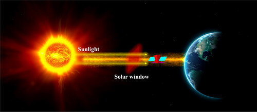
Figure 2. Propagation path of rays emitted from the solar window.

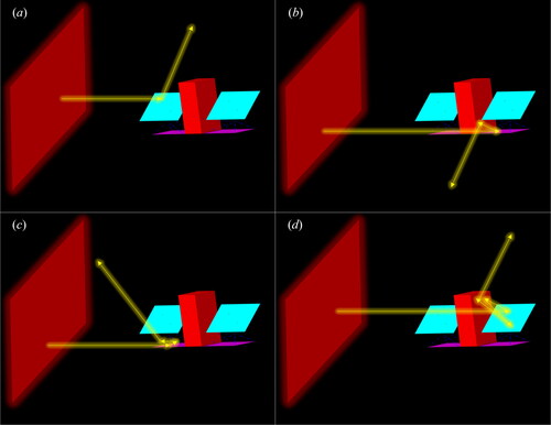
Figure 3. Comparison of two processes for solving solar radiation external heat flux considering parameter uncertainty, left (conventional) and right (based on EHFE equation).

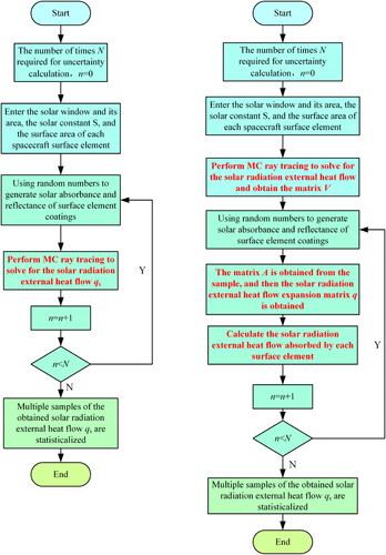
Figure 4. Spacecraft thermal analysis model.

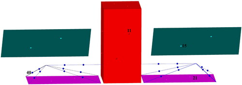
Figure 5. Spacecraft position map.

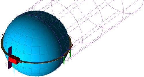
Figure 6. Split-edge violin plots of surface elements absorbing solar radiation external heat flux.

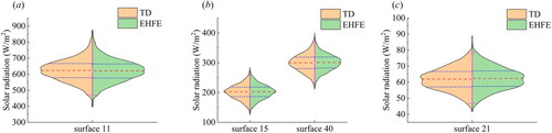
Figure 7. Probability distribution of the surface elements absorbing solar radiation external heat flux.

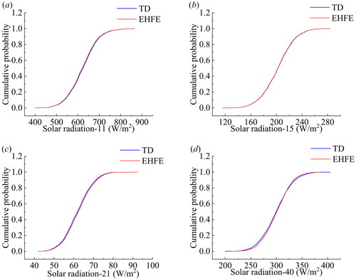
Figure 8. Probability density plots of the surface elements absorbing solar radiation external heat flux.

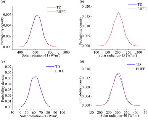
Table 1. Orbit and attitude parameters.

Parameters	Numerical value
Semimajor axis/km	6878
Eccentricity	0
Orbit inclination/(°)	0
Attitude	Z-axis to ground orientation

Table 2. Spacecraft experimental analysis surface element numbers and their components.

Number of surface elements	Spacecraft components belonging to surface elements
11	Satellite body
15	Solar panel
21	Antennae
40	Truss

Table 3. Distribution of the uncertainty variables.

Input parameters	Distribution type	Average value	Standard deviation
Satellite body solar absorption rate	Normal distribution	0.46	0.05
Antennae solar absorption rate	Normal distribution	0.65	0.05
Solar panel solar absorption rate	Normal distribution	0.41	0.05
Truss solar absorption rate	Normal distribution	0.56	0.05

Table 4. Mean and standard deviation of the absorbed solar radiation external heat flux for the two model surface elements.

	TD model (W/m^2)	EHFE equation (W/m^2)	Relative error (%)	Absolute error (W/m^2)
Surface Element 11 mean	622.53	620.24	0.368	2.290
Surface Element 11 standard deviation	67.56	67.34	0.316	0.214
Surface Element 15 mean	201.83	202.08	0.123	0.249
Surface Element 15 standard deviation	24.08	24.13	0.188	0.045
Surface Element 21 mean	62.00	62.42	0.690	0.428
Surface Element 21 standard deviation	7.00	7.05	0.607	0.042
Surface Element 40 mean	299.66	300.48	0.274	0.820
Surface Element 40 standard deviation	28.89	26.76	7.389	2.135

Table 5. Confidence interval of the solar radiation external heat flux for both models.

		TD model (W/m^2)	EHFE equation (W/m^2)	Relative error (%)	Absolute error (W/m^2)
95.40%	Lower confidence interval for Surface Element 11	487.12	485.11	0.41	2.01
	Upper confidence interval for Surface Element 11	760.91	758.27	0.35	2.64
	Lower confidence interval for Surface Element 15	153.10	153.48	0.25	0.38
	Upper confidence interval for Surface Element 15	249.69	250.05	0.15	0.36
	Lower confidence interval for Surface Element 21	48.35	48.61	0.53	0.26
	Upper confidence interval for Surface Element 21	76.21	76.52	0.41	0.31
	Lower confidence interval for Surface Element 40	243.01	246.99	1.64	3.97
	Upper confidence interval for Surface Element 40	359.26	355.34	1.09	3.92
99.70%	Lower confidence interval for Surface Element 11	415.58	413.03	0.61	2.55
	Upper confidence interval for Surface Element 11	850.14	849.77	0.04	0.37
	Lower confidence interval for Surface Element 15	131.65	132.09	0.33	0.44
	Upper confidence interval for Surface Element 15	271.15	272.06	0.34	0.91
	Lower confidence interval for Surface Element 21	43.97	44.37	0.93	0.41
	Upper confidence interval for Surface Element 21	84.14	84.81	0.80	0.67
	Lower confidence interval for Surface Element 40	220.57	224.10	1.60	3.53
	Upper confidence interval for Surface Element 40	385.44	381.97	0.90	3.47

Table 6. Time required for the calculation of the uncertainty solar radiation external heat flux for each method.

	Uncertainty solar radiation external heat flux
TD(s)	1660
EHFE equation (s)	823
Speed multiplier (multiple)	2.01

Table 7. Comparison of the results of the standard deviation of the uncertain solar radiation external heat flux for element 40 under different ray number conditions.

	TD model (W/m^2)	EHFE equation (W/m^2)	Relative error (%)	Absolute error (W/m^2)
4 × 10^6 rays Surface Element 40 standard deviation	28.89	26.76	7.389	2.135
2 × 10^7 rays Surface Element 40 standard deviation	27.22	26.09	4.127	1.123

References

- K. Cao and J. Baker, “Multimode heat transfer in a near-space environment,” Heat Transf. Eng., vol. 31, no. 1, pp. 70–82, 2010. DOI: 10.1080/01457630903263499.
- F. Yang, Q. Sun and L. Cheng, “Thermal simulation of alpha magnetic spectrometer in orbit,” Numer. Heat Transf, A: Appl., vol. 83, no. 4, pp. 417–439, 2022. DOI: 10.1080/10407782.2022.2091891.
- M. Donabedian, “Thermal uncertainty margins for cryogenic sensor systems,” presented at the 26th Thermophysics Conference, 1991. p. 1426. DOI: 10.2514/6.FDC.
- T. Ishimoto and J. T. Bevans, “Temperature variance in spacecraft thermal analysis,” J. Spacecr. Rock., vol. 5, no. 11, pp. 1372–1376, 1968. DOI: 10.2514/3.29491.
- J. R. Howell, “Monte Carlo treatment of data uncertainties in thermal analysis,” J. Spacecr. Rock., vol. 10, no. 6, pp. 411–414, 1973. DOI: 10.2514/3.61899.
- D. P. Thunnissen, S. K. Au and G. T. Tsuyuki, “Uncertainty quantification in estimating critical spacecraft component temperatures,” J. Thermophys. Heat Transf., vol. 21, no. 2, pp. 422–430, 2007. DOI: 10.2514/1.23979.
- A. Gómez-San-Juan, I. Pérez-Grande and A. Sanz-Andrés, “Uncertainty calculation for spacecraft thermal models using a generalized SEA method,” Acta Astronaut., vol. 151, pp. 691–702, 2018. DOI: 10.1016/j.actaastro.2018.05.045.
- Y. Xiong, L. Guo, Y. Yang and H. Wang, “Intelligent sensitivity analysis framework based on machine learning for spacecraft thermal design,” Aerosp. Sci. Technol., vol. 118, pp. 106927, 2021. DOI: 10.1016/j.ast.2021.106927.
- H. Kato, M. Ando and M. Fukuzoe, “Toward uncertainty quantification in satellite thermal design,” Aerosp. Technol. Jpn., vol. 17, no. 2, pp. 134–141, 2019. DOI: 10.2322/tastj.17.134.
- R. G. Regis, “Evolutionary programming for high-dimensional constrained expensive black-box optimization using radial basis functions,” IEEE Trans. Evol. Computat., vol. 18, no. 3, pp. 326–347, 2014. DOI: 10.1109/TEVC.2013.2262111.
- J. P. Kleijnen, “Kriging metamodeling in simulation: a review,” Eur. J. Oper. Res., vol. 192, no. 3, pp. 707–716, 2009. DOI: 10.1016/j.ejor.2007.10.013.
- Z. Han, Y. Zhang, C. Song and K. Zhang, “Weighted gradient-enhanced kriging for high-dimensional surrogate modeling and design optimization,” Aiaa J., vol. 55, no. 12, pp. 4330–4346, 2017. DOI: 10.2514/1.J055842.
- J. Qian, J. Yi, Y. Cheng, J. Liu and Q. Zhou, “A sequential constraints updating approach for Kriging surrogate model-assisted engineering optimization design problem,” Eng. Comput., vol. 36, no. 3, pp. 993–1009, 2020. DOI: 10.1007/s00366-019-00745-w.
- R. Datta and R. G. Regis, “A surrogate-assisted evolution strategy for constrained multi-objective optimization,” Expert Syst. Appl., vol. 57, pp. 270–284, 2016. DOI: 10.1016/j.eswa.2016.03.044.
- Z. Song, B. T. Murray, B. Sammakia and S. Lu, “Multi-objective optimization of temperature distributions using artificial neural networks,” 13th InterSociety Conference on Thermal and Thermomechanical Phenomena in Electronic Systems, 2012. IEEE, pp. 1209–1218. DOI: 10.1109/ITHERM.2012.6231560.
- A. Altan, Ö. Aslan and R. Hacıoğlu, “Real-time control based on NARX neural network of hexarotor UAV with load transporting system for path tracking,” 2018 6th International Conference on Control Engineering & Information Technology (CEIT), 2018. IEEE, pp. 1–6. DOI: 10.1109/CEIT.2018.8751829.
- R. Kromanis and P. Kripakaran, “Support vector regression for anomaly detection from measurement histories,” Adv. Eng. Inform., vol. 27, no. 4, pp. 486–495, 2013. DOI: 10.1016/j.aei.2013.03.002.
- S. Rahmani, M. Ebrahimi and A. Honaramooz, “A surrogate-based optimization using polynomial response surface in collaboration with population-based evolutionary algorithm,” in Advances in Structural and Multidisciplinary Optimization: Proceedings of the 12th World Congress of Structural and Multidisciplinary Optimization (WCSMO12) 12, 2018, Cham, Switzerland: Springer, pp. 269–280. DOI: 10.1007/978-3-319-67988-4_19.
- X. Fu, Y. Hua, W. Ma, H. Cui and Y. Zhao, “An innovative external heat flow expansion formula for efficient uncertainty analysis in spacecraft earth radiation heat flow calculations,” Aerospace, vol. 10, no. 7, pp. 605, 2023. DOI: 10.3390/aerospace10070605.
- X. Fu, L. Liang, W. Ma, H. Cui and Y. Zhao, “Efficient uncertainty analysis of external heat flux of solar radiation with external heat flux expansion for spacecraft thermal design,” Aerospace, vol. 10, no. 8, pp. 672, 2023. DOI: 10.3390/aerospace10080672.
- A. Jurkowski, R. Paluch, M. Wójcik and A. Klimanek, “Sensitivity analysis and uncertainity quantification of thermal model for data processing unit dedicated for nanosatellite space missions,” 2022 28th International Workshop on Thermal Investigations of ICs and Systems (THERMINIC), 2022: IEEE, pp. 1–5. DOI: 10.1109/THERMINIC57263.2022.9950639.
- C. Zheng, J. Qi, J. Song and L. Cheng, “Effects of the rotation of International Space Station main radiator on suppressing thermal anomaly of Alpha Magnetic Spectrometer caused by flight attitude adjustment,” Appl. Therm. Eng., vol. 171, pp. 115100, 2020. DOI: 10.1016/j.applthermaleng.2020.115100.
- A. Kersch, W. Morokoff and A. Schuster, “Radiative heat transfer with quasi-Monte Carlo methods,” Transport. Theor. Statist. Phys, vol. 23, no. 7, pp. 1001–1021, 1994. DOI: 10.1080/00411459408203537.
- Y. Liu, G.-H. Li and L.-X. Jiang, “A new improved solution to thermal network problem in heat-transfer analysis of spacecraft,” Aerosp. Sci. Technol., vol. 14, no. 4, pp. 225–234, 2010. DOI: 10.1016/j.ast.2009.12.001.
- M. Yuan, Y.-Z. Li, Y. Sun and B. Ye, “The space quadrant and intelligent occlusion calculation methods for the external heat flux of China space Station,” Appl. Therm. Eng., vol. 212, pp. 118572, 2022. DOI: 10.1016/j.applthermaleng.2022.118572.
- W. Yang, H. Cheng and A. Cai, “Thermal analysis for folded solar array of spacecraft in orbit,” Appl. Therm. Eng., vol. 24, no. 4, pp. 595–607, 2004. DOI: 10.1016/j.applthermaleng.2003.10.005.
- A. Farrahi and I. Pérez-Grande, “Simplified analysis of the thermal behavior of a spinning satellite flying over sun-synchronous orbits,” Appl. Therm. Eng., vol. 125, pp. 1146–1156, 2017. DOI: 10.1016/j.applthermaleng.2017.07.033.
- I. Krainova, A. Nenarokomov, I. Nikolichev, D. Titov and V. Chumakov, “Radiative heat fluxes in orbital space flight,” J. Eng. Thermophys., vol. 31, no. 3, pp. 441–457, 2022. DOI: 10.1134/S1810232822030079.
- P. Li, H-e Cheng and W-b Qin, “Numerical simulation of temperature field in solar arrays of spacecraft in low earth orbit,” Numer. Heat Transf., A: Appl., vol. 49, no. 8, pp. 803–820, 2006. DOI: 10.1080/10407780500503904.
- C. Zheng, J. Qi, J. Song and L. Cheng, “Numerical investigation on the thermal performance of Alpha Magnetic Spectrometer main radiators under the operation of International Space Station,” Numer. Heat Transf., A: Appl., vol. 77, no. 5, pp. 538–558, 2020. DOI: 10.1080/10407782.2020.1713634.
- S. Selvadurai, A. Chandran, D. Valentini and B. Lamprecht, “Passive thermal control design methods, analysis, comparison, and evaluation for micro and nanosatellites carrying infrared imager,” Appl. Sci.-Basel, vol. 12, no. 6, pp. 2858, 2022. DOI: 10.3390/app12062858.