An energy-conservative DG-FEM approach for solid–liquid phase change

Abstract

We present a discontinuous Galerkin method for melting/solidification problems based on the “linearized enthalpy approach,” which is derived from the conservative form of the energy transport equation and does not depend on the use of a so-called mushy zone. We use the symmetric interior penalty method and the Lax–Friedrichs flux to discretize diffusive and convective terms, respectively. Time is discretized with a second-order implicit backward differentiation formula, and two outer iterations with second-order extrapolation predictors are used for the coupling of the momentum and energy. The numerical method was validated with three different benchmark cases, i.e., the one-dimensional Stefan problem, octadecane melting in a square cavity and gallium melting in a rectangular cavity. The performance of the method was quantified based on the L² norm error and the number of iterations needed to convergence the energy equation at each time step. For all three validation cases, a mesh convergence rate of approximately O(h) was obtained, which is below the expected accuracy of the numerical method. Only for the gallium melting case, the use of a higher-order method proved to be beneficial. The results from the present numerical campaign demonstrate the promise of the discontinuous Galerkin finite element method for modeling certain solid–liquid phase change problems where large gradients in the flow field are present or the phase change is highly localized, however, further enhancement of the method is needed to fully benefit from the use of a higher-order numerical method when solving solid–liquid phase change problems.

Keywords:

• Energy-conservative discontinuous Galerkin method
• linearized enthalpy approach
• solid–liquid phase change

1. Introduction

Melting and solidification phase change plays an important role in a wide range of disciplines, amongst which metallurgy [1–3], thermal management, and latent heat storage [4–7], reduction of waste plastic [8] and the design of the Molten Salt Fast Reactor (MSFR) [9–11]. The numerical solution of melting and solidification problems is non-trivial, due to the mathematical complexity of solving the moving boundary problem, with a discontinuity in both the enthalpy and the temperature gradient at the solid–liquid interface [12]. Moreover, most melting and solidification problems of industrial significance are coupled to other physics, such as fluid flow, solid settling [13], neutronics [11], or turbulence modeling [14–19].

Whilst many different approaches exist to modeling melting and solidification problems (such as transformed grid approach [20, 21], the level-set method [22–25], and the phase field method [26–31]), we chose to restrict ourselves to implicit fixed grid approaches. Here, “implicit fixed grid” refers to the solution of the melting/solidification problem on a single fixed domain where the solid–liquid interface is tracked implicitly, i.e., the interface position is inferred from the enthalpy or temperature field at the current time step, instead of being obtained by solving a separate equation. This approach has the advantage of being applicable to a wide range of melting and solidification problems, not requiring mesh deformation, coordinate transformation, or grid generation and not having to calculate interface curvatures, impose boundary conditions at the interface or having to deal with complex thermodynamic derivations. For this reason, the implicit fixed grid approach has been the most popular choice for modeling macroscale phase change phenomena in industrial applications.

The most widely used implicit fixed grid methods are the apparent heat capacity method, which accounts for the latent heat release through a modified form of the heat capacity around the melting point [32–34], and the source-based enthalpy approach [35–37] where the latent heat release is captured through a source term. The tradeoff between these two methods is speed versus robustness. Whilst the apparent heat capacity method is fast, a naive implementation of the method (such as using too large time steps, a too-small mushy zone or a too-fine mesh without the proper precautions) may lead to an incorrect amount of the latent heat being released, and therefore, a deteriorated solution quality [38]. Conversely, the source-based enthalpy approach requires an iterative procedure and may be slow to converge.

To overcome these deficiencies, the “linearized enthalpy approach” (also referred to as “a generalized enthalpy approach” or “an optimum approach”) has been developed [39–43]. With this approach, the volumetric enthalpy is linearized around the latest temperature values and the energy equation is iterated until convergence has been reached. Compared to the source-based approach, the “linearized enthalpy approach” requires significantly less nonlinear iterations to converge the energy equation [42]. Unlike the apparent heat capacity method or the source-based approach, the “linearized enthalpy approach” used in this work is based on the conservative form of the energy transport equation and the conservation of thermal energy is verified through the imposed convergence criterion. Finally, the “linearized enthalpy approach” does not depend on the use of a so-called “mushy zone,” eliminating the energy error arising from the smearing of the latent heat peak.

An important drawback of implicit fixed grid methods is their relatively low accuracy in capturing the melting or solidification front. This is mainly due to the difficulty of resolving the discontinuity in the enthalpy and temperature solutions within the cell, leading to a maximum mesh convergence rate of O(h) [44–46]. Therefore, a very fine mesh may be needed to obtain grid-independent results [20, 21, 47]. To improve the computational efficiency of the implicit fixed grid approach for modeling melting and solidification problems, recent studies have investigated the use of finite elements with adaptive mesh refinement algorithms [48, 49], using extended finite element methods [24, 50, 51] or using discontinuous Galerkin finite element methods (DG-FEM) [52–55] for solving solid–liquid phase change problems, which is the focus of the present work.

Discontinuous Galerkin methods have gained interest over the last decade as an attractive numerical method for computational fluid dynamics, due to its combination of desired features of both the finite volume (FVM) and finite element (FEM) methods, such as local conservation, the possibility for upwinding, an arbitrarily high order of discretization and high geometric flexibility [56–58]. In addition, the high locality of the numerical scheme makes the discontinuous Galerkin method efficient for parallelization [58]. Recent advances in the applicability of DG-FEM methods to computational fluid dynamics include the simulation of turbulent flow with a high-order discontinuous Galerkin method and RANS or LES turbulence modeling [59–63], the development of discontinuous Galerkin methods for low-Mach number flow [64, 65], the simulation of multiphase flows [66, 67] and a DG-FEM multiphysics solver for simulating the Molten Salt Fast Reactor [58]. When coupled to a melting and solidification model, DG-FEM is expected to offer a more reliable capture of nonlinear phase change phenomena as compared to the finite-volume method [52]. Indeed, Schroeder and Lube [53] obtained qualitatively similar results on a mesh that was 14 times coarser as compared to the mesh used in a similar finite volume numerical benchmark study [47]. For these reasons, DG-FEM is an attractive numerical method for modeling solid–liquid phase change problems.

The present work introduces the Symmetric Interior Penalty - Discontinuous Galerkin (SIP-DG) discretization of the “linearized enthalpy approach” with the aim of developing an accurate and computationally efficient numerical method for modeling melting and solidification. Previous investigations employing the DG-FEM method to simulate melting and/or solidification problems used the apparent heat capacity method [52, 55] or the source-based enthalpy approach [53] for modeling the phase transition. To the best of our knowledge, this is the first time the “linearized enthalpy” approach has been implemented in a DG-FEM framework. An important novelty here is the imposition of thermal energy conservation through the convergence criterion. Furthermore, the present approach is thoroughly validated through comparison against three different benchmark cases (i.e., the one-dimensional Stefan problem, octadecane melting in a square enclosure and gallium melting in a rectangular enclosure). Finally, the performance of the discontinuous Galerkin with “linearized enthalpy approach” method is quantified by calculating and comparing mesh convergence rates for two different element orders.

The rest of this article is organized as follows. Section 2 presents the governing equations and the boundary conditions that close them. Section 3 introduces the semi-discrete variational formulation with the discontinuous Galerkin method. Section 4 describes the temporal discretization scheme, with special attention devoted to the time-integration of the nonlinear energy transport equation and the coupling of the energy and momentum transport equations. The results from the three benchmark cases and accompanying numerical performance metrics are presented in Section 5. Finally, the conclusions and recommendations for future work based on the obtained results are given in Section 6.

2. Governing equations

We consider the energy and the momentum transport equations in conservative form and use the volumetric enthalpy as the main variable. As such, the energy transport equation is written as (1) $$\frac{\partial H}{\partial t}+\nabla ·\left(\mathit{u}H\right)=\nabla ·\left(\lambda \nabla T\right),$$(1) where H is the volumetric enthalpy, u is the velocity, λ is the thermal conductivity, and T is the temperature.

The energy transport equation contains two unknowns, the volumetric enthalpy in the accumulation and the convection terms and the temperature in the diffusion term, coupled through the enthalpy–temperature relationship. For most heat transfer problems, the enthalpy–temperature relationship is smooth and the temperature gradient in the diffusion term may be expressed in terms of the enthalpy ($\nabla T=\frac{1}{\rho c_p}\nabla H$) with ρ being the density and c_p the specific heat capacity, hereby eliminating the temperature as the unknown and resulting in a linear energy transport equation that may be solved by standard solution methods. However, for solid–liquid phase change problems, the enthalpy–temperature relationship is nonsmooth resulting in a nonlinear energy transport equation. For this reason, dedicated numerical methods are needed for modeling solid–liquid phase change.

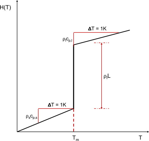
Figure 1 depicts the enthalpy-temperature relationship for isothermal solid–liquid phase change. For temperatures below the melting point ($T<T_m$), the enthalpy temperature derivative is equal to $\frac{dH}{dT}={\rho }_s{c}_{p,s}.$ For temperatures above the melting point ($T>T_m$), the enthalpy temperature derivative is equal to $\frac{dH}{dT}={\rho }_l{c}_{p,l}.$ Here, the subscripts “s” and “l” refer to the solid and liquid phase, respectively. At the melting point, the volumetric enthalpy has a jump discontinuity with a magnitude of ${\rho }_{l}L$ where L is the latent heat and ${\rho }_{l}L$ is the energy required for a unit volume of solid at the melting temperature to be transformed into liquid.

Figure 1. Enthalpy temperature relationship, for isothermal solid–liquid phase change. Here, ρ is the density, c_p is the specific heat capacity, L is the latent heat and the subscripts “l” and “s” refer to the liquid and the solid phases, respectively.

Assuming constant thermophysical properties in each phase, and neglecting the volume expansion effect as a consequence of the difference in densities between the solid and the liquid, the enthalpy–temperature relationship is written as a piece-wise continuous function: (2) $$T(H)=\{\begin{array}{c}\frac{H}{{\rho }_s{c}_{p,s}},\hspace{1em}H\le {\rho }_s{c}_{p,s}{T}_m\hfill \\ T_m,\hspace{1em}{\rho }_s{c}_{p,s}{T}_m<H<{\rho }_s{c}_{p,s}{T}_m+{\rho }_{l}L\hfill \\ T_m+\frac{H-({\rho }_s{c}_{p,s}{T}_m+{\rho }_{l}L)}{{\rho }_l{c}_{p,l}},\hspace{1em}H\ge {\rho }_s{c}_{p,s}{T}_m+{\rho }_{l}L.\hfill \end{array}$$(2)

Following the recommendation of Ref. [68], who experienced numerical instabilities when using the convection of the total enthalpy coupled to their implementation of the “linearized enthalpy approach,” we use a “sensible enthalpy only” formulation for the convection term. Theory predicts that for isothermal solid–liquid phase change, under the condition that no solid-settling occurs and possible volume expansion effects due to different solid and liquid densities are neglected, the velocity at the solid–liquid interface is equal to zero, and therefore, the convection of the latent heat is also equal to zero [37]. In practice, however, the finite element approximation of the volumetric enthalpy by piece-wise continuous functions will lead to an inevitable smearing of the latent heat peak within an element and the convection of the latent heat will no longer be zero after the finite element discretization. This “false numerical convection of latent heat” may result in poor convergence and deteriorated quality of results. Following the rational of the source-based approach [37], the convection of the total enthalpy is split into a sensible and a latent heat contribution: $\nabla ·(\mathit{u}{H}_{\text{tot}})=\nabla ·(\mathit{u}{H}_{\text{sens}})+\nabla ·(\mathit{u}\alpha L).$ Here, α is the liquid fraction (not to be confused with the thermal diffusivity), defined as (3) $$\alpha (T)=\{\begin{array}{c}0,\hspace{1em}T\le T_m\hfill \\ 1,\hspace{1em}T>T_m.\hfill \end{array}$$(3)

Since the latent heat contribution is considered equal to zero, only the sensible contribution remains. The sensible contribution is expressed in terms of the temperature: $\nabla ·(\mathit{u}{H}_{\text{sens}})={\rho }_l{c}_{p,l}\nabla ·(\mathit{u}T).$ The “sensible enthalpy only” formulation of the energy transport equation is thus written as (4) $$\frac{\partial H}{\partial t}+{\rho }_l{c}_{p,l}\nabla ·\left(\mathit{u}T\right)=\nabla ·\left(\lambda \nabla T\right).$$(4)

For the momentum equation, we consider incompressible flow and a Newtonian fluid with constant viscosity, and use the Boussinesq approximation to model the effect of buoyancy. The Darcy source term approach is used to enforce the no-slip condition at the solid–liquid interface position. This approach is most commonly used and has demonstrated better performance compared to other approaches such as the switch-off and variable viscosity techniques [12, 36]. The momentum equation, thus, reads (5) $$\begin{array}{c}\frac{\partial \left({\rho }_l\mathit{u}\right)}{\partial t}+\nabla ·\left(\mathit{u}\otimes \left({\rho }_l\mathit{u}\right)\right)=\nabla ·\left[\mu \left(\nabla \mathit{u}+{\left(\nabla \mathit{u}\right)}^T\right)\right]-\nabla p\\ +{\rho }_l\mathit{g}\beta (T-T_m)-C\frac{{\left(1-\alpha \right)}^2}{{\alpha }^3+b}\mathit{u}.\end{array}$$(5) The large parameter C > 0 in the Darcy source term is responsible for the attenuation of the velocity in the solid phase. b > 0 is a small parameter to prevent division by zero when the liquid fraction α becomes equal to zero.

Finally, the continuity equation for incompressible flow reads (6) $$\nabla ·\mathit{u}=0.$$(6)

To close the system of coupled volumetric enthalpy transport and momentum transport equations, a set of boundary conditions and initial conditions are supplied. In the present work, the boundary $\partial \Omega$ is decomposed into two pairwise disjoint sets ${\Gamma }^D$ and ${\Gamma }^N$ such that $\partial \Omega ={\Gamma }^D\cup {\Gamma }^N.$ On the Dirichlet boundary ${\Gamma }^D$ the temperature is given, i.e., $T=T^D,$ whereas on the Neumann boundary ${\Gamma }^N$ the heat flux is specified, i.e., $\lambda \nabla T·\mathit{n}=q.$ Here, n is the outward unit normal vector of $\partial \Omega .$ The no-slip condition $\mathit{u}=0$ is imposed on the entire boundary $\partial \Omega .$ Initially, the temperature in the whole domain Ω is known, and the fluid is at rest, i.e., $\mathit{u}=0$ and p = 0 at t = 0.

3. Spatial discretization

This section describes the spatial discretization of the volumetric enthalpy and the mass flux transport equations with the discontinuous Galerkin finite element method. First, we introduce the basic definitions required for writing the variational formulation. Let Ω be the computational domain and $\Gamma ={\Gamma }^D\cup {\Gamma }^N$ its boundary. The domain is meshed into a set of nonoverlapping elements ${\mathcal{T}}_h,$ with ${\mathcal{F}}^i,{\mathcal{F}}^D,$ and ${\mathcal{F}}^N$ being the set of interior, Dirichlet and Neumann boundary faces, respectively. For each element $\mathcal{T}\in {\mathcal{T}}_h$ we assign a set of faces ${\mathcal{F}}^T,$ and for each face $\mathcal{F}$ we assign a set of neighboring elements ${\mathcal{T}}_h^F.$ All faces $\mathcal{F}\in {\mathcal{F}}^i\cup {\mathcal{F}}^D\cup {\mathcal{F}}^N$ are assigned a unit normal vector ${\mathit{n}}^F,$ which has an arbitrary but fixed direction for all interior faces and coincides with the unit outward normal vector n for the boundary faces.

We use a hierarchical set of orthogonal modal basis functions (normalized Legendre polynomials to be specific) to approximate the unknown variables on ${\mathcal{T}}_h.$ The solution space within each element is the span of all polynomials up to an order $\mathcal{P}$ and is written as (7) $${\mathcal{V}}_{h,\varphi }:=\left\{v\in L^2(\Omega )\hspace{1em}|\hspace{1em}v{|}_T\in {\mathbb{P}}_{{\mathcal{P}}_{\varphi }},\hspace{1em}\forall \mathcal{T}\in {\mathcal{T}}_h\right\},$$(7) where $\varphi$ is a generic unknown variable and ${\varphi }_h$ represents its FEM approximation. The basis functions are continuous within each element, but discontinuous at the interface between two neighboring elements. As such, the trace of ${\varphi }_h$ on the interior faces ${\mathcal{F}}^i$ is not unique, and we need to define the average and the jump operator, these are $\left\{{\varphi }_h\right\}=\frac{1}{2}({\varphi }_h^{+}+{\varphi }_h^{-})$ and $\left[\left[{\varphi }_h\right]\right]={\varphi }_h^{+}-{\varphi }_h^{-},$ respectively. Here, for any point r on an interior face $\mathcal{F}\in {\mathcal{F}}^i,$ the function traces ${\varphi }_h^{+}$ and ${\varphi }_h^{-}$ are defined as (8) $${\varphi }_h^{\pm }\left(\mathit{r}\in F\right)=\underset{\zeta \downarrow 0}{\lim }{\varphi }_h\left(\mathit{r}\pm \zeta {\mathit{n}}^F\right).$$(8)

3.1. Variational formulation

The semi-discrete variational formulation of the coupled system of transport equations is obtained by replacing the mass flux, pressure, volumetric enthalpy, and temperature with their DG-FEM approximations (${\mathit{m}}_h,p_h,H_h,T_h$), by multiplying Eqs. (4)–(6)(6) $$\nabla ·\mathit{u}=0.$$(6) with the test functions ${\mathit{v}}_h\in {\mathcal{V}}_{h,m}^d,q_h\in {\mathcal{V}}_{h,p},$ and $w_h\in {\mathcal{V}}_{h,T,H},$ respectively, and subsequently integrating over the whole domain. Note that the superscript d denotes the dimensionality of the vector space to which the DG-FEM approximation of the mass flux belongs. To close the system of equations, the enthalpy–temperature coupling needs to be included. With these considerations, the semi-discrete variational formulation reads $$\begin{array}{c}\text{Find}\hspace{1em}{m}_h\in {\mathcal{V}}_{h,m}^d\hspace{1em}\text{and}\hspace{1em}{p}_h\in {\mathcal{V}}_{h,p,H,T}\hspace{1em}\text{and}\hspace{1em}{H}_h\in {\mathcal{V}}_{h,p,H,T}\hspace{1em}\text{and}\hspace{1em}{T}_h\in {\mathcal{V}}_{h,p,H,T}\hspace{1em}\\ \text{such}\hspace{1em}\text{that}\hspace{1em}\forall v_h\in {\mathcal{V}}_{h,m}^d\hspace{1em}\text{and}\hspace{1em}\forall q_h,\forall w_h\in {\mathcal{V}}_{h,p,H,T},\end{array}$$ (9a) $$\begin{array}{c}\sum _{\mathcal{T}\in {\mathcal{T}}_h}{\int }_{\mathcal{T}}{\mathit{v}}_h·\frac{\partial {\mathit{m}}_h}{\partial t}+a^{\text{conv}}({\mathit{u}}_h,{\mathit{m}}_h,{\mathit{v}}_h)+a^{\text{diff}}({\mathit{m}}_h,{\mathit{v}}_h)+a^{\text{div}}({\mathit{v}}_h,p_h)\\ +a^{\text{source}}({\mathit{m}}_h,{\mathit{v}}_h)=l^{\text{conv}}({\mathit{u}}_h,{\mathbf{v}}_h)+l^{\text{diff}}\left({\mathit{v}}_h\right)+l^{\text{source}}({\mathit{v}}_h,T_h)\end{array}$$(9a) (9b) $$a^{\text{div}}({\mathit{m}}_h,q_h)=l^{\text{div}}(q_h)$$(9b) (9c) $$\begin{array}{c}\sum _{\mathcal{T}\in {\mathcal{T}}_h}{\int }_{\mathcal{T}}{w}_h\frac{\partial H_h}{\partial t}+a^{\text{conv}}({\mathit{m}}_h,T_h,w_h)+a^{\text{diff}}(T_h,w_h)\hfill \\ =l^{\text{conv}}({\mathit{u}}_h,w_h)+l^{\text{diff}}(w_h)\hfill \end{array}$$(9c) (9d) $$T_h=T(H_h).$$(9d)

By solving the variational formulation of the coupled system of transport equations, the numerical mass-flux m_h, the pressure p_h, the volumetric enthalpy H_h, and the temperature T_h are obtained. As opposed to the source-based enthalpy approach employed by Ref. [53], the present variational formulation follows directly from the conservative form of the transport equations. In addition, the present formulation does not depend on the use of an artificial smearing of the latent heat peak through the introduction of a so-called mushy-zone, and directly preserves the enthalpy-temperature coupling through inclusion in the system of equations. The nonlinear coupling between the enthalpy and the temperature does not allow for a straightforward solution of the discretized energy transport equation. Therefore, we chose an iterative solution method for the energy equation, based on the work of Refs. [39, 40, 42]. The iterative solution of the energy equation is described in more detail in Subsection 4.1.

In the present work, a mixed-order discretization for the mass-flux and the enthalpy, temperature, and pressure was used (i.e., ${\mathcal{P}}_{p,H,T}={\mathcal{P}}_m-1$). The mixed-order formulation for the mass-flux and pressure (i.e., ${\mathcal{P}}_{p,T}={\mathcal{P}}_m-1$) is inf-sup stable and therefore no pressure stabilization terms are needed in the discretized continuity equation [58, 69] as opposed to using an equal-order formulation. In addition, it has been shown that the solution space of a transported scalar quantity (in the present work, the enthalpy and the temperature) must be a subset of the solution space of the pressure [58, 65]. The reason is that the continuity equation is weighted by the pressure basis functions (see Eq. (9)(9a) $$\begin{array}{c}\sum _{\mathcal{T}\in {\mathcal{T}}_h}{\int }_{\mathcal{T}}{\mathit{v}}_h·\frac{\partial {\mathit{m}}_h}{\partial t}+a^{\text{conv}}({\mathit{u}}_h,{\mathit{m}}_h,{\mathit{v}}_h)+a^{\text{diff}}({\mathit{m}}_h,{\mathit{v}}_h)+a^{\text{div}}({\mathit{v}}_h,p_h)\\ +a^{\text{source}}({\mathit{m}}_h,{\mathit{v}}_h)=l^{\text{conv}}({\mathit{u}}_h,{\mathbf{v}}_h)+l^{\text{diff}}\left({\mathit{v}}_h\right)+l^{\text{source}}({\mathit{v}}_h,T_h)\end{array}$$(9a) ), and therefore, the convective discretization in the scalar transport equation can only be consistent up to order ${\mathcal{P}}_p.$ For this reason, we selected ${\mathcal{P}}_{H,T}={\mathcal{P}}_p$), resulting in the final mixed-order formulation ${\mathcal{P}}_{p,H,T}={\mathcal{P}}_m-1.$

We will now specify the convection, diffusion, divergence, and source term operators in the discretized momentum and continuity equations. The treatment of the convection and diffusion operators in the energy equation proceeds along the same lines. The treatment of the time-operator will be described in detail in Section 4.

3.2. Convective term

The discretization of the convective term is given by (10) $$\begin{array}{c}{a}^{\text{conv}}({\mathit{u}}_{\mathit{h}},{\mathit{m}}_h,{\mathit{v}}_h)=-\sum _{\mathcal{T}\in {\mathcal{T}}_h}{\int }_{\mathcal{T}}{\mathit{m}}_h·\left({\mathit{u}}_h·\nabla \right)v_h+\sum _{\mathcal{F}\in {\mathcal{F}}^i}{\int }_{\mathcal{F}}\left[\left[{\mathit{v}}_h\right]\right]{\mathcal{H}}^F\left({\mathit{u}}_h,{\mathit{m}}_h\right)\\ +\sum _{\mathcal{F}\in {\mathcal{F}}^N}{\int }_{\mathcal{F}}\left({\mathit{n}}^F·{\mathit{u}}_h\right){\mathit{m}}_h·{\mathit{v}}_h+\sum _{\mathcal{F}\in {\mathcal{F}}^D}{\int }_{\mathcal{F}}\max \left(0,{\mathit{n}}^F·{\mathit{u}}_h^D\right){\mathit{m}}_h·{\mathit{v}}_h\end{array}$$(10) (11) $$l^{\text{conv}}({\mathit{u}}_h,{\mathit{v}}_h)=-\sum _{\mathcal{F}\in {\mathcal{F}}^D}{\int }_{\mathcal{F}}\min \left(0,{\mathit{n}}^F·{\mathit{u}}_h^D\right){\mathit{m}}_h^D·{\mathit{v}}_h,$$(11) where ${\mathcal{H}}^F$ is the numerical flux function defined on an internal face $\mathcal{F}\in {\mathcal{F}}^i.$ In this work, the Lax–Friedrichs flux is used [70]: (12) $${\mathcal{H}}^F\left({\mathit{u}}_h,{\mathit{m}}_h\right)=\frac{{\alpha }^F\left({\mathit{u}}_h\right)}{2}\left[\left[{\mathit{m}}_h\right]\right]+{\mathit{n}}^F·\left\{{\mathit{u}}_h\otimes {\mathit{m}}_h\right\},$$(12) where α^F is evaluated point-wise at face $\mathcal{F}$ through (13) $${\alpha }^F\left({\mathit{u}}_h\right)=\Lambda \max \left(\left|{\mathit{n}}^F·{\mathit{u}}_h^{+}\right|,\left|{\mathit{n}}^F·{\mathit{u}}_h^{-}\right|\right)$$(13) with Λ = 2 for the momentum equation and Λ = 1 for the energy equation.

3.3. Diffusive term

Following [58, 65], we discretize the diffusive term using the Symmetric Interior Penalty (SIP) method. We limit ourselves to laminar incompressible flow and consider a Newtonian fluid with constant viscosity. For this reason, we present the standard SIP bilinear form instead of the generalization outlined in Ref. [65]: (14) $$\begin{array}{c}{a}^{\text{diff}}({\mathit{m}}_h,{\mathbf{v}}_h)=\sum _{\mathcal{T}\in {\mathcal{T}}_h}{\int }_{\mathcal{T}}\frac{\mu }{\rho }\nabla {\mathit{m}}_h·\nabla {\mathit{v}}_h+\sum _{\mathcal{F}\in {\mathcal{F}}^i\cup {\mathcal{F}}^D}{\int }_{\mathcal{F}}{\eta }^F\left[\left[{\mathit{m}}_h\right]\right]\left[\left[{\mathit{v}}_h\right]\right]\\ -\sum _{\mathcal{F}\in {\mathcal{F}}^i\cup {\mathcal{F}}^D}{\int }_{\mathcal{F}}{\mathit{n}}^F·\left(\left[\left[{\mathit{v}}_h\right]\right]\left\{\frac{\mu }{\rho }\nabla {\mathit{m}}_h\right\}+\left[\left[{\mathit{m}}_h\right]\right]\left\{\frac{\mu }{\rho }\nabla {\mathit{v}}_h\right\}\right)\end{array}$$(14) (15) $$l^{\text{diff}}({\mathit{v}}_h)=\sum _{\mathcal{F}\in {\mathcal{F}}^D}{\int }_F\left({\eta }^F{\mathit{m}}^D·{\mathit{v}}_h-{\mathit{m}}_h^D·\frac{\mu }{\rho }\nabla {\mathit{v}}_h·{\mathit{n}}^F\right).$$(15)

An optimum value of the penalty parameter is calculated through [71] (16) $${\eta }^F=\max \left({\frac{\mu }{\rho }}^{+},{\frac{\mu }{\rho }}^{-}\right)\max \left(\text{card}\left({\mathcal{F}}^T\right)\frac{{\mathfrak{E}}_{\mathcal{P},\mathcal{T}}}{{\mathfrak{L}}_{\mathcal{T}}}\right),$$(16) where $\text{card}({\mathcal{F}}^T)$ represents the number of faces of element $\mathcal{T}$ and ${\mathfrak{E}}_{\mathcal{P},\mathcal{T}}$ is a factor which takes into account the polynomial order of the finite element basis and test functions and the type of elements used: (17) $${\mathfrak{E}}_{\mathcal{P},\mathcal{T}}=\{\begin{array}{c}{\left(P+1\right)}^2,\hspace{1em}\text{for}\mathrm{ }\text{quadrilaterals}\mathrm{ }\text{and}\mathrm{ }\text{hexahedra}\hfill \\ \frac{\left(P+1\right)\left(P+d\right)}{d},\hspace{1em}\text{for}\mathrm{ }\text{simplices}.\hfill \end{array}$$(17) ${\mathfrak{L}}_{\mathcal{T}}$ is a length scale defined as (18) $${\mathfrak{L}}_{\mathcal{T}}=f\frac{{\left|\left|T\right|\right|}_{\mathit{leb}}}{{\left|\left|F\right|\right|}_{\mathit{leb}}}$$(18) where ${\left|\left|T\right|\right|}_{\mathit{leb}}$ indicates the Lebesgue measure of the element, and ${\left|\left|F\right|\right|}_{\mathit{leb}}$ indicates the Lebesgue measure of the face, respectively. Finally, f = 2 for boundary faces, and f = 1 for internal faces. For the SIP discretization of the diffusive term in the energy equation, we substitute λ for $\frac{\mu }{\rho }$ and substitute T_h for ${\mathit{m}}_h.$

3.4. Continuity terms

The discretized continuity equation consists of the following discrete divergence operator and right-hand side term [72, 73]: (19) $$a^{\text{div}}({\mathit{u}}_h,q_h)=-\sum _{\mathcal{T}\in {\mathcal{T}}_h}{\int }_{\mathcal{T}}q\nabla ·{\mathit{u}}_h+\sum _{\mathcal{F}\in {\mathcal{F}}^i\cup F^D}{\int }_{\mathcal{F}}\left\{q\right\}\left[\left[{\mathit{u}}_h\right]\right]·{\mathit{n}}^F$$(19) (20) $$l^{\text{div}}(q)=\sum _{\mathcal{F}\in {\mathcal{F}}^D}{\int }_{\mathcal{F}}q\left({\mathit{u}}^D·{\mathit{n}}^F\right).$$(20)

3.5. Source terms

The momentum equation contains two source terms, i.e., the Darcy source term responsible for the attenuation of the velocity at the solid–liquid interface and the Boussinesq approximation responsible for modeling natural convection. The Darcy source term is imposed implicitly through the bilinear operator $a^{\text{source}}({\mathit{m}}_h,{\mathit{v}}_{\mathit{h}}):$ (21) $$a^{\text{source}}\left({\mathit{m}}_h,{\mathit{v}}_{\mathit{h}}\right)=\sum _{\mathcal{T}\in {\mathcal{T}}_h}{\int }_{\mathcal{T}}C\frac{\left(1-\alpha \right)}{{\alpha }^3+b}\frac{{\mathit{m}}_h·{\mathit{v}}_{\mathit{h}}}{{\rho }_l}.$$(21)

For the liquid fraction, a finite element approximation of the same order as the mass flux is used. To obtain the finite element approximation of the liquid fraction, the liquid fraction is calculated from the temperature at each quadrature point (see Eq. (3)(3) $$\alpha (T)=\{\begin{array}{c}0,\hspace{1em}T\le T_m\hfill \\ 1,\hspace{1em}T>T_m.\hfill \end{array}$$(3) ), and the values at the quadrature points are subsequently projected onto the finite element basis.

The Boussinesq approximated is imposed explicitly through the linear right-hand side term $l^{\text{source}}({\mathit{v}}_{\mathit{h}},T_h):$ (22) $$l^{\text{source}}\left({\mathit{v}}_{\mathit{h}},T_h\right)=\sum _{\mathcal{T}\in {\mathcal{T}}_h}{\int }_{\mathcal{T}}{\rho }_l\beta \left(T_h-T_m\right){\mathit{v}}_{\mathit{h}}·\mathit{g}.$$(22)

4. Temporal discretization and numerical solution procedure

In this work, implicit time-stepping is performed using the backward differentiation formulae (BDF) [62, 64, 73]. The time derivatives for a generic unknown quantity $\varphi$ and for a constant time step $\Delta t$ is therefore written as (23) $$\frac{\partial \varphi }{\partial t}\approx \frac{{\gamma }_0}{\Delta t}{\varphi }^{n+1}+\sum _{j=1}^{\mathcal{M}}\frac{{\gamma }_j}{\Delta t}{\varphi }^{n+1-j},$$(23) where $\mathcal{M}$ is the order of the BDF scheme. In the present work, the second-order BDF scheme is used, with ${\gamma }_0=3/2,{\gamma }_1=-2,$ and ${\gamma }_2=1/2.$ Special treatment is used for the temporal discretization and time-integration of the enthalpy transport equation, as is explained in Subsection 4.1. The coupled momentum and continuity equations are solved in a segregated way using a pressure correction method (see Subsection 4.2). The full solution algorithm, including the coupling between the energy, momentum, and continuity equations, is described in Subsection 4.3.

4.1. Iterative solution of energy equation

Applying BDF2 time-integration (and assuming a constant time step), the discretized energy accumulation term is written as (24) $$\sum _{\mathcal{T}\in {\mathcal{T}}_h}{\int }_{\mathcal{T}}{w}_h\frac{\partial H_h}{\partial t}=\sum _{\mathcal{T}\in {\mathcal{T}}_h}{\int }_{\mathcal{T}}{w}_h\frac{3H_h^{n+1}-4H_h^n+H_h^{n-1}}{2\Delta t}.$$(24)

Inserting the discretized energy accumulation term into the variational formulation of the energy equation results in the following form: (25) $$\begin{array}{c}\sum _{\mathcal{T}\in {\mathcal{T}}_h}{\int }_{\mathcal{T}}{w}_h\frac{3H_h^{n+1}-4H_h^n+H_h^{n-1}}{2\Delta t}+a^{\text{conv}}({\mathit{m}}_h,T_h^{n+1},w_h)+a^{\text{diff}}(T_h^{n+1},w_h)=\\ l^{\text{conv}}({\mathit{u}}_h,w_h)+l^{\text{diff}}(w_h).\end{array}$$(25)

This equation is highly nonlinear in the unknown $H_h^{n+1},$ due to the discontinuous nature of the enthalpy-temperature relationship (see Eq. (2)(2) $$T(H)=\{\begin{array}{c}\frac{H}{{\rho }_s{c}_{p,s}},\hspace{1em}H\le {\rho }_s{c}_{p,s}{T}_m\hfill \\ T_m,\hspace{1em}{\rho }_s{c}_{p,s}{T}_m<H<{\rho }_s{c}_{p,s}{T}_m+{\rho }_{l}L\hfill \\ T_m+\frac{H-({\rho }_s{c}_{p,s}{T}_m+{\rho }_{l}L)}{{\rho }_l{c}_{p,l}},\hspace{1em}H\ge {\rho }_s{c}_{p,s}{T}_m+{\rho }_{l}L.\hfill \end{array}$$(2) ) and therefore cannot be solved in a straightforward manner. Building on the work of Refs. [39, 40, 42], we expand the unknown $H_h^{n+1}$ around the temperature: (26) $$H_h^{n+1,i+1}=H_h^{n+1,i}+\frac{dH}{dT}{|}_{n+1,i}\left(T^{n+1,i+1/2}-T^{n+1,i}\right),$$(26) where the superscript i + 1 refers to the new iteration, and $i+1/2$ refers to an intermediate value between two iterations. Inserting the expansion into the discretized energy equation yields the “linearized” discretized energy equation: (27) $$\begin{array}{c}\sum _{\mathcal{T}\in {\mathcal{T}}_h}{\int }_{\mathcal{T}}{w}_h\frac{3H_h^{n+1,i}-4H_h^n+H_h^{n-1}}{2\Delta t}+\sum _{\mathcal{T}\in {\mathcal{T}}_h}{\int }_{\mathcal{T}}\frac{dH}{dT}{|}_{n+1,i}{w}_h\frac{3T_h^{n+1,i+1/2}-3T_h^{n+1,i}}{2\Delta t}\\ +a^{\text{conv}}({\mathit{m}}_h,T_h^{n+1,i+1/2},w_h)+a^{\text{diff}}(T_h^{n+1,i+1/2},w_h)=l^{\text{conv}}({\mathit{u}}_h,w_h)+l^{\text{diff}}(w_h).\end{array}$$(27)

The linearized discretized energy equation contains only the intermediate temperature $T_h^{n+1,i+1/2}$ as the unknown variable. Solving the linearized energy equation for the intermediate temperature may be seen as a single step in a Newton iteration. The remaining challenge is now to define a suitable approximation of the enthalpy-temperature derivative, which is undefined at the melting point.

In this work, we use the following formulation: (28) $$\frac{dH}{dT}\approx \{\begin{array}{c}\omega {\rho }_s{c}_{p,s},\hspace{1em}T\le T_m\hfill \\ \omega {\rho }_l{c}_{p,l},\hspace{1em}T>T_m,\hfill \end{array}$$(28) where ω is an overrelaxation factor (1.5 was used in the present work) with the sole purpose of speeding up the convergence. Upon convergence, the linearization term $(\frac{dH}{dT}{|}_{n+1,i}(T^{n+1,i+1/2}-T^{n+1,i}))$ approaches zero. Therefore, for a strict enough convergence criterion, the exact form of the enthalpy-temperature derivative has a negligible effect on the result of the numerical solution, and the use of the current approximation is justified [40]. Finally, we would like to mention that instead of updating the thermal conductivity at each iteration according to the latest position of the solid–liquid interface, the thermal conductivity at the newest time step is estimated using extrapolation from the previous two time steps (see Subsection 4.3) and is, therefore, kept constant during the nonlinear enthalpy–temperature iterations.

The iterative solution procedure is described by the following steps:

1. Initialize the enthalpy at the new time step $H^{n+1,i}$ using the extrapolation from the previous time steps (see Eq. (38)(38) $${\varphi }^{n+1,*}=2{\varphi }^n-{\varphi }^{n-1}.$$(38) ).

2. Solve the discretized linearized energy transport equation (Eq. (27)(27) $$\begin{array}{c}\sum _{\mathcal{T}\in {\mathcal{T}}_h}{\int }_{\mathcal{T}}{w}_h\frac{3H_h^{n+1,i}-4H_h^n+H_h^{n-1}}{2\Delta t}+\sum _{\mathcal{T}\in {\mathcal{T}}_h}{\int }_{\mathcal{T}}\frac{dH}{dT}{|}_{n+1,i}{w}_h\frac{3T_h^{n+1,i+1/2}-3T_h^{n+1,i}}{2\Delta t}\\ +a^{\text{conv}}({\mathit{m}}_h,T_h^{n+1,i+1/2},w_h)+a^{\text{diff}}(T_h^{n+1,i+1/2},w_h)=l^{\text{conv}}({\mathit{u}}_h,w_h)+l^{\text{diff}}(w_h).\end{array}$$(27) ) to obtain the solution for the intermediate temperature $T_h^{n+1,i+1/2}.$

3. Update the volumetric enthalpy at the quadrature points applying the Taylor linearization: (29) $$H_h^{n+1,i+1}{|}_{qp}=H_h^{n+1,i}{|}_{qp}+{\frac{dH}{dT}}^{n+1,i}\left(T_h^{n+1,i+1/2}-T_h^{n+1,i}\right){|}_{qp}.$$(29)

4. At the quadrature points, calculate the temperature from the updated enthalpy values through the enthalpy–temperature relationship (see Eq. (2)(2) $$T(H)=\{\begin{array}{c}\frac{H}{{\rho }_s{c}_{p,s}},\hspace{1em}H\le {\rho }_s{c}_{p,s}{T}_m\hfill \\ T_m,\hspace{1em}{\rho }_s{c}_{p,s}{T}_m<H<{\rho }_s{c}_{p,s}{T}_m+{\rho }_{l}L\hfill \\ T_m+\frac{H-({\rho }_s{c}_{p,s}{T}_m+{\rho }_{l}L)}{{\rho }_l{c}_{p,l}},\hspace{1em}H\ge {\rho }_s{c}_{p,s}{T}_m+{\rho }_{l}L.\hfill \end{array}$$(2) ): (30) $$T_h^{n+1,i+1}=T\left(H_h^{n+1,i+1}\right).$$(30)

5. Calculate the solution coefficients of the enthalpy and temperature at the latest iteration, by projecting the values at the quadrature points onto the finite element basis for each element: (31) $$\begin{array}{c}\mathit{M}{H}_h^{n+1,i+1}=\sum _{qp=1}^n\left(w{|}_{qp}{H}^{n+1,i+1}{|}_{qp}{v}_h\right),\hspace{1em}\mathit{M}{T}_h^{n+1,i+1}\left(T_h^{n+1,i+1}{v}_h\right)\\ =\sum _{qp=1}^n\left(w{|}_{qp}T{|}_{qp}{v}_h\right),\end{array}$$(31)

where $w{|}_{qp}$ are the quadrature weights and M is the mass matrix.

• Check whether the convergence criterion (see Eq. (32)(32) $$\max \left(\frac{\mathit{res}}{E_{\text{tot}}},{\left(\frac{{\int }_{\Omega }\left({\left[T_h^{n+1,i+1}-T_h^{n+1,i}\right]}^2\right)}{{\int }_{\Omega }\left({\left[T_h^{n+1,i+1}\right]}^2\right)}\right)}^{1/2}\right)<\mathit{tol}.$$(32) ) is satisfied. If not, return to step 2. If yes, move to the solution of the momentum equation (see Figure 2).

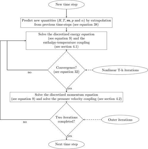
Figure 2. Flowchart of the solution algorithm, including the nonlinear temperature–enthalpy iterations and the coupling of the energy and the momentum equations.

Through our approach, the energy equation is solved in conservative form through a series of nonlinear enthalpy–temperature iterations, within a prescribed tolerance. The advantages of our approach for solving melting and/or solidification problems as opposed to the apparent heat capacity method or the source-based enthalpy approach are an inherent conservation of thermal energy, no dependency on use of a so-called mushy zone for smearing the latent heat peak, and a comparatively fast convergence of the energy equation per time step.

4.1.1. Convergence criterion

To ensure the final solution of the linearized energy transport equation corresponds to the solution of the original energy transport equation (see Eq. (4)(4) $$\frac{\partial H}{\partial t}+{\rho }_l{c}_{p,l}\nabla ·\left(\mathit{u}T\right)=\nabla ·\left(\lambda \nabla T\right).$$(4) ), a suitable convergence criterion is defined: (32) $$\max \left(\frac{\mathit{res}}{E_{\text{tot}}},{\left(\frac{{\int }_{\Omega }\left({\left[T_h^{n+1,i+1}-T_h^{n+1,i}\right]}^2\right)}{{\int }_{\Omega }\left({\left[T_h^{n+1,i+1}\right]}^2\right)}\right)}^{1/2}\right)<\mathit{tol}.$$(32)

This convergence criterion depends on two parts. The second part is the L² norm of the temperature difference between the current and the previous iteration. The justification for this part of the convergence criterion is that upon convergence, the linearization term should be equal to zero (see Eq. (26)(26) $$H_h^{n+1,i+1}=H_h^{n+1,i}+\frac{dH}{dT}{|}_{n+1,i}\left(T^{n+1,i+1/2}-T^{n+1,i}\right),$$(26) ). In other words, the L² norm of the temperature difference between the current and the previous iteration should be minimized. The first part of the convergence criterion may be considered an energy conservation check. This is done by inserting the solution vectors into the original discretized energy equation (i.e., prior to linearization, see Eq. (9))(9a) $$\begin{array}{c}\sum _{\mathcal{T}\in {\mathcal{T}}_h}{\int }_{\mathcal{T}}{\mathit{v}}_h·\frac{\partial {\mathit{m}}_h}{\partial t}+a^{\text{conv}}({\mathit{u}}_h,{\mathit{m}}_h,{\mathit{v}}_h)+a^{\text{diff}}({\mathit{m}}_h,{\mathit{v}}_h)+a^{\text{div}}({\mathit{v}}_h,p_h)\\ +a^{\text{source}}({\mathit{m}}_h,{\mathit{v}}_h)=l^{\text{conv}}({\mathit{u}}_h,{\mathbf{v}}_h)+l^{\text{diff}}\left({\mathit{v}}_h\right)+l^{\text{source}}({\mathit{v}}_h,T_h)\end{array}$$(9a) and selecting the zeroth-order polynomial v_h = 1 as test function. Therefore, all terms containing the gradients and/or jumps of the test-function are equal to zero (except for the jumps at the boundaries) and the residual may be defined as: (33) $$\begin{array}{c}\mathit{res}=\sum _{\mathcal{T}\in {\mathcal{T}}_h}{\int }_{\mathcal{T}}{v}_h·\frac{3H_h^{n+1,i+1}-4H_h^n+H_h^{n-1}}{2\Delta t}\\ +\sum _{\mathcal{F}\in {\mathcal{F}}^N}{\int }_{\mathcal{F}}\left({\mathit{n}}^F·{\mathit{u}}_h\right){\rho }_l{c}_{p,l}{T}_h^{n+1,i+1}·v_h+\sum _{\mathcal{F}\in {\mathcal{F}}^D}{\int }_{\mathcal{F}}\max \left(0,{\mathit{n}}^F·{\mathit{u}}_h^D\right){\rho }_l{c}_{p,l}{T}_h^{n+1,i+1}·v_h\\ +\sum _{\mathcal{F}\in {\mathcal{F}}^D}{\int }_{\mathcal{F}}{\eta }^F\left[\right[T_h^{n+1,i+1}\left]\right]\left[\right[{\mathbf{v}}_h\left]\right]-\sum _{\mathcal{F}\in {\mathcal{F}}^D}{\int }_{\mathcal{F}}\left(\left\{\right\{\lambda \nabla T_h^{n+1,i+1}\left\}\right\}·{\mathit{n}}^F\left[\right[v_h\left]\right]\right)\\ +\sum _{\mathcal{F}\in {\mathcal{F}}^D}{\int }_{\mathcal{F}}\min \left(0,{\mathbf{n}}^F·{\mathit{u}}_h^D\right){\rho }_l{c}_{p,l}{T}_h^D·v_h-\sum _{\mathcal{F}\in {\mathcal{F}}^D}{\int }_{\mathcal{F}}\left({\eta }^F{T}_h^D·v_h\right).\end{array}$$(33) The residual is thus a measure of the energy loss or gain after each iteration, which is a measure of how far the solution to the linearized equation is from satisfying thermal energy conservation. The residual is scaled with the total thermal energy in the system to represent a relative error.

4.2. Pressure correction method

The coupled continuity and momentum equations are solved in a segregated way, applying the following pressure correction scheme [58, 65, 73]:

1. Obtain a predictor for the mass flux m by solving the linear system which corresponds to the semi-discrete form (see Eq. (9)) (34) $$\left(\frac{{\gamma }_0}{\Delta t}\mathbb{M}+\mathbb{N}\right){\widehat{\mathit{m}}}^{n+1}=-{\mathbb{D}}^T{p}^n+\mathit{f}.$$(34) Here, $\mathbb{M}$ is the mass matrix, $\mathbb{N}$ contains the implicit parts of the discrete convection and diffusion terms, $\mathbb{D}$ is the discrete divergence operator and f collects all the explicit terms (i.e., explicit terms from the discretization of the time derivative, boundary conditions, and source terms). The convective term is linearized by replacing the convective field ${\mathit{u}}^{n+1}$ with the predictor $\frac{{\mathit{m}}^{n+1,*}}{{\rho }_l}.$

2. Solve a Poisson equation to obtain the pressure-difference at the new time step (35) $$\left(\frac{\Delta t}{{\gamma }_0}\mathbb{D}{\mathbb{M}}^{-1}{\mathbb{D}}^T\right)\delta p^{n+1}=\mathbb{D}{\widehat{\mathit{m}}}^{n+1}-b_p,$$(35) where b_p represents the fully discrete right-hand side of the continuity equation (see Eq. (20)(20) $$l^{\text{div}}(q)=\sum _{\mathcal{F}\in {\mathcal{F}}^D}{\int }_{\mathcal{F}}q\left({\mathit{u}}^D·{\mathit{n}}^F\right).$$(20) ). Subsequently, the pressure may be updated, (36) $$p^{n+1}=p^n+\delta p^{n+1}.$$(36)

3. Correct the mass flux, such that it satisfies the discrete continuity equation (37) $${\mathit{m}}^{n+1}={\widehat{\mathit{m}}}^{n+1}-\frac{\Delta t}{{\gamma }_0}{\mathbb{M}}^{-1}{\mathbb{D}}^T\delta p^{n+1}.$$(37)

4.3. Full solution algorithm

The full set of discretized transport equations is solved using a one-way coupling method between the energy and the momentum equation. The algorithm to find the solution vectors ${\mathit{m}}^{n+1},{\mathit{p}}^{n+1},{\mathit{H}}^{n+1},$ and ${\mathit{T}}^{n+1}$ at a new time step n + 1 consists of the following steps (also see Figure 2).

1. Obtain predictors for the temperature T, enthalpy H, mass flux m, pressure p, liquid fraction α, and thermal conductivity λ, using a second-order extrapolation from previous time steps: (38) $${\varphi }^{n+1,*}=2{\varphi }^n-{\varphi }^{n-1}.$$(38)

2. Solve the discretized energy equation through a series of Newton iterations until convergence is achieved, as described in Subsection 4.1.

3. Solve the coupled momentum and continuity equations using the pressure correction method described in Subsection 4.2.

4. Repeat steps 3 and 4 for a number of n outer iterations. In this work, 2 outer iterations were deemed sufficient based on a sensitivity analysis.

4.4. Implementation and numerical solution

The DG-FEM formulation of the linearized enthalpy approach for simulating melting and solidification heat transfer problems was validated with three different test cases: the 1D Stefan problem, octadecane melting in a square enclosure [5] and gallium melting in a rectangular enclosure [1]. The linearized enthalpy approach was implemented in the in-house DG-FEM based computational fluid dynamics solver DGFlows. A hierarchical set of orthogonal modal basis functions (normalized Legendre polynomials to be specific) was used and all integrals were evaluated with a Gaussian quadrature set with polynomial accuracy of $3P_m-1$ [74, 75]. The meshes were generated with the open-source software tool Gmsh [76]. METIS [77] is used to partition the mesh, and the MPI-based software library PETSc [78] is used to assemble and solve all linear systems with iterative Krylov methods. The pressure-Poisson system is solved with the conjugate gradient method and a block jacobi preconditioner, where the submatrix within each MPI process is preconditioned with an incomplete Cholesky decomposition. The linear systems for the linearized enthalpy and momentum equations are solved with GMRES, with a block Jacobi preconditioner and successive over-relaxation for the submatrix within each MPI process. To reduce the required computational time, the pressure matrix and its preconditioner are only assembled and computed once (since the pressure matrix is the same at each time step [58]), and the Krylov solvers are initialized with the solution predictors (see Section 4) to speed up the convergence.

5. Results and discussion

5.1. Case 1: 1D Stefan problem

The one-dimensional Stefan problem was chosen for the first test case because the absence of convection and the presence of an analytical solution enabled a step-wise validation of the proposed numerical method, as well as a quantitative evaluation of the error in the numerical solution. We, thus, consider a one-dimensional rod of length $l=0.05\mathrm{m},$ with a temperature of $T(x,t=0)=278\mathrm{K}.$ At t > 0, the temperature at the left side is suddenly lowered below the melting temperature: $T(0,t)=268\mathrm{K}<T_m$ and the right side is described by a homogeneous Neumann boundary condition, $\frac{\partial T}{\partial x}{|}_{t,L}=0.$ The phase change material matches the thermophysical properties of water (see Table 1). The same density is used for the solid and the liquid phases, to avoid any issues regarding volume expansion and mass conservation.

Table 1. Thermophysical properties used in the one-dimensional Stefan problem (corresponding to the thermophysical properties of water).

	Solid	Liquid
Density, kg m^−3	1000	1000
Specific heat capacity, J kg^−1	4200	2100
Thermal conductivity, W m^−1 K^−1	2.16	0.575
Latent heat, J kg^−1	333000
Melting temperature, K	273

The entire problem is described by one pair of heat conduction equations, i.e., one heat conduction equation for the solid phase and one for the liquid phase [35]: (39) $$\{\begin{array}{c}\frac{\partial T_l}{\partial t}={\alpha }_l\frac{{\partial }^2{T}_l}{\partial x^2},\hspace{1em}0\le x<s(t)\hfill \\ \frac{\partial T_s}{\partial t}={\alpha }_s\frac{{\partial }^2{T}_s}{\partial x^2},\hspace{1em}x\ge s(t).\hfill \end{array}$$(39)

The displacement of the solid–liquid interface in time is described by the following two conditions, where “s” represents the solid–liquid interface: (40) $$\{\begin{array}{c}{T}_l=T_s=T_m\hfill \\ {\rho }_{s}L\frac{ds(t)}{dt}=k_s\frac{\partial T_s}{\partial x}{|}_{x=s(t)}-k_l\frac{\partial T_l}{\partial x}{|}_{x=s(t)}.\hfill \end{array}$$(40)

The analytical solution to the 1D Stefan problem is well known and given by Voller and Cross [35] (41) $$s(t)=2\lambda {\left({\alpha }_{s}t\right)}^{1/2},$$(41) where λ is the solution to the following transcendental equation: (42) $$\frac{\lambda L{\pi }^{1/2}}{c_s\left[T_m-T(0,t)\right]}=\frac{\hspace{0.17em}\exp \hspace{0.17em}\left(-{\lambda }^2\right)}{\text{erf}\left(\lambda \right)}-\frac{k_l}{k_s}\frac{{\alpha }_s^{1/2}\left[T(x,0)-T_m\right]\hspace{0.17em}\exp \hspace{0.17em}\left(-{\alpha }_s{\lambda }^2/{\alpha }_l\right)}{{\alpha }_l^{1/2}\left[T_m-T_{(}0,t\right]\text{erfc}\left(\lambda {\left(k_s/k_l\right)}^{1/2}\right)}.$$(42)

The analytical solution for the temperature is given by (43) $$T=\{\begin{array}{c}\frac{T_m-T(0,t)}{\text{erf}\left(\lambda \right)}\text{erf}\left(\frac{x}{2{\left({\alpha }_{s}t\right)}^{1/2}}\right)+T(0,t),\hspace{1em}x<s(t)\hfill \\ T_m,\hspace{1em}x=s(t)\hfill \\ T(x,0)-\frac{T(x,0)-T_m}{\text{erfc}\left(\lambda \left({\alpha }_s/{\alpha }_l{}^{1/2}\right)\right)}\text{erfc}\left(\frac{x}{2{\left({\alpha }_{l}t\right)}^{1/2}}\right),\hspace{1em}x>s(t).\hfill \end{array}$$(43)

Figure 3 shows the numerical versus the analytical solution, for both the temperature field and the solid–liquid interface position. 128 equally sized linear elements and BDF2 time-integration with a time step of $\Delta t=0.1s$ were used. The tolerance was set to $\mathit{tol}={10}^{-6}.$ The numerical solid–liquid interface position was found based on $H_{\mathit{num}}={\rho }_s{c}_{p,s}{T}_m+0.5{\rho }_{l}L.$ For the temperature field, excellent agreement with the analytical results was observed and it is nearly impossible to distinguish the numerical and analytical solutions by eye. Conversely, although the overall agreement with the analytical solution is good, the numerical solution for the solid–liquid interface position “jumps” in time. This is due to the numerical solid–liquid interface being localized at one of the element edges, until the enthalpy has jumped past the latent heat peak. The “time-jumping” of the numerical solid–liquid interface position is therefore inherent to the discontinuous Galerkin finite element discretization.

Figure 3. (a) Temperature field at 100, 250, 500, and 1000 s. (b) Solid–liquid interface position. Numerical vs. analytical solution for a 1D Stefan problem, with 128 linear elements, and a time step of $\Delta t=0.1\mathrm{s}$ with BDF2 time-integration. $\mathit{tol}={10}^{-6}.$ See Ref. [79] for the implementation of the solution of the 1D Stefan problem with the discontinuous Galerkin method and the linearized enthalpy approach in an inhouse Fortran code. The raw data of the 1D Stefan problem is included in a Zenodo repository [80].

In Figure 4, the L² norm of the error (44) $${\left(\frac{{\int }_{\Omega }\left({\left[T_{\text{num}}^{*}-T_{\text{an}}^{*}\right]}^2\right)}{{\int }_{\Omega }\left({\left[T_{\text{an}}^{*}\right]}^2\right)}\right)}^{1/2}$$(44) versus the number of elements is depicted. Here, the normalized temperatures are used, i.e., $T^{*}=\frac{T-T_C}{T_H-T_c}$ with $T_c=268\mathrm{K}$ and $T_H=278\mathrm{K}.$ The errors continue to decrease with an increasing amount of elements and approach very small values, indicating that the numerical solution converges to the analytical solution. For both the linear and the quadratic elements, approximately linear ($O(h])$) convergence rates were achieved. Note that the elements are only discontinuous at the element edges: within each element, a continuous finite element approximation is used. Since the solid–liquid interface is most of the time located somewhere within an element, we believe the suboptimal linear convergence rate is a consequence of the use of continuous polynomials for approximating the discontinuities in the enthalpy and temperature fields at the interface. Also recall the “trapping” of the solid–liquid interface position at the element edges, until both nodal enthalpy values have moved past the latent heat peak. The current results are in line with theoretical predictions that the optimal convergence rate for a Stefan problem with a finite element method and implicit tracking of the solid–liquid interface is O(h) [44]. Possibly, a faster mesh convergence could be obtained using adaptive mesh refinement in the vicinity of the solid–liquid interface [49] or an extended finite element method [24].

Figure 4. Mesh convergence rate based on the L² norm of the error in the temperature field. The total time was 250 s and the time step was $\Delta t=0.1\mathrm{s}.$ The raw data of the 1D Stefan problem is included in a Zenodo repository [80].

5.2. Case 2: Melting of octadecane in a square container

For the second benchmark case, we consider a square cavity of dimensions $H\times W=40\text{mm}\times 40\text{mm},$ filled with n-octadecane as the phase-change material (PCM). At the initial temperature of $T_0=298.15\mathrm{K},$ the entire PCM is solid. At t = 0, the left wall is suddenly heated to $T_H=308.15\mathrm{K}.$ The right wall is kept constant at $T_C=298.15\mathrm{K}$ and the rest of the walls are adiabatic. The thermophysical properties of n-octadecane are given in Table 2. We chose this particular benchmark case for the following two reasons:

Table 2. Thermophysical properties of n-octadecane [5].

	Solid	Liquid
Density, kg m^−3	867	775.6
Specific heat capacity, J kg^−1	1900	2240
Thermal conductivity, W m^−1 K^−1	0.32	0.15
Latent heat, J kg^−1	243680
Melting temperature, K	301.15
Thermal expansion coefficient, 1/K	$8.36·{10}^{-4}$
Dynamic viscosity, Pas	$3.75·{10}^{-3}$

1. The availability of recent experimental measurements, with relatively well described boundary conditions, including PIV measurements of the flowfield [5].

2. The availability of a recent numerical investigation with a linearized enthalpy approach and the finite volume method (FVM) [42], to compare the performance of the present method against.

Figure 5 depicts the absolute velocity contours at, respectively, 1 and 2 h after the onset of melting as measured experimentally using PIV (top two images) and numerically (bottom two images). Qualitatively, a good agreement was observed between the experimental data and the simulation results. The onset of the natural circulation loop, as seen in the PIV results, is well captured by the numerical method. As a consequence of the natural convection flow, the heat transfer to the solid–liquid interface is enhanced and the rate of melting is accelerated.

Figure 5. Absolute velocity contours for melting of n-octadecane in a square enclosure, at, respectively, 3600 s and 7200 s. Qualitative comparison between experimental campaign (top) and numerical campaign (bottom). Numerical campaign performed with “linearized enthalpy approach” coupled to a SIP-DG numerical method. 200 × 200 $P=\{2,1,1,1\}$ elements were used. Time-integration was performed with the BDF2 finite difference scheme and $\Delta t=0.25\mathrm{s}.$ The raw data of the octadecane melting case is included in a Zenodo repository [80].

Figure 6 shows the results from a mesh convergence analysis, for both the solid–liquid interface position and the temperature plotted on the line $y=0\text{mm}$ through the center of the domain. All meshes consist of equally sized quadrilateral elements. Two different hierarchical sets of orthogonal basis functions were used, respectively, $P=\{2,1,1,1\}$ and $P=\{3,2,2,2\}$ for the mass flux, pressure, enthalpy, and temperature. Both sets of polynomial orders displayed visually similar results for $P=\{2,1,1,1\}$ and $P=\{3,2,2,2\}$ with the finer meshes of 200 × 200 and 400 × 400 elements.

Figure 6. Mesh convergence study based on interface position and temperature at the line $y=0\text{mm}.$ Two sets of finite element polynomial orders are selected, these are $P=\{2,1,1,1\}$ and $P=\{3,2,2,2\}.$ BDF2 time-stepping with $\Delta t=0.5\mathrm{s}$ was used for a total simulation time of 3600 s. The raw data of the octadecane melting case is included in a Zenodo repository [80]. (a) Interface position, P = {2,1,1,1} (b) Interface position, P = {3,2,2,2} (c) Temperature, P = {2,1,1,1} (d) Temperature, P = {3,2,2,2}

To provide insight on the mesh convergence rates, Table 3 depicts the average number of inner iterations, the total liquid fraction, and the L²-norms of errors in the temperature, enthalpy and the absolute velocity (see Eq. (44)(44) $${\left(\frac{{\int }_{\Omega }\left({\left[T_{\text{num}}^{*}-T_{\text{an}}^{*}\right]}^2\right)}{{\int }_{\Omega }\left({\left[T_{\text{an}}^{*}\right]}^2\right)}\right)}^{1/2}$$(44) ). Quantitative mesh convergence studies for solid–liquid phase change problems are rare and to the best of our knowledge this is the first time such a study has been performed for the solution of solid–liquid phase change problems with a discontinuous Galerkin method. The number of inner iterations do not grow excessively with an increasing mesh-size, although for the finest meshes of 400 × 400 elements a relatively large number of iterations was needed to obtain convergence. This was probably a consequence of keeping the time step constant at $\Delta t=0.5,$ for the higher mesh resolutions a smaller time step could be more suitable. The differences in the total liquid fraction are small, even between the finest and the coarsest mesh, which can possibly be attributed to the good energy conservation properties of the current numerical method. For the L² norms, the normalized quantities were used, i.e., $T^{*}=\frac{T-T_C}{T_H-T_c}$ with $T_c=298.15\mathrm{K}$ and $T_H=308.15\mathrm{K}$ and $|u{|}^{*}=\frac{\left|u\right|}{\max (|u|)}.$ Since now we do not have an analytical solution to compare to, the numerical solution for the finest mesh (i.e., 400 × 400 and $P=\{3,2,2,2\}$) was used as the reference solution. For both the $P=\{2,1,1,1\}$ and the $P=\{3,2,2,2\}$ meshes, the L² error norms for the first 3 meshes (less than 100 × 100 elements) appeared to decrease slowly (less than O(h)), whilst the error decreased with a rate close to O(h) from the 100 × 100 elements mesh onwards.

Table 3. Relevant quantities from the mesh convergence analysis for the octadecane melting in a square cavity case.

Polynomial order	Mesh size	Average number of inner iterations	Total liquid fraction	L^2T	L^2H	L^2U
$P=\{2,1,1,1\}$	25 × 25	4.95, 2.29	0.212	2.24(–1)	3.89(–1)	4.99(–1)
	50 × 50	6.64, 1.89	0.210	1.62(–1)	2.58(–1)	3.25(–1)
	100 × 100	9.27, 1.93	0.213	1.04(–1)	1.95(–1)	2.09(–1)
	200 × 200	13.03, 1.85	0.212	4.39(–2)	1.12(–1)	9.97(–2)
	400 × 400	24.95, 2.27	0.218	2.50(–2)	8.35(–2)	6.86(–2)
$P=\{3,2,2,2\}$	25 × 25	5.67, 1.83	0.190	2.74(–1)	3.89(–1)	6.10(–1)
	50 × 50	7.00, 1.86	0.202	1.84(–1)	2.92(–1)	4.12(–1)
	100 × 100	9.51, 1.78	0.210	1.01(–1)	1.93(–1)	2.40(–1)
	200 × 200	13.59, 1.89	0.213	3.87(–2)	1.04(–1)	9.66(–2)
	400 × 400	33.92, 4.03	0.216	N/A	N/A	N/A

BDF2 time-integration with a time step of $\Delta t=0.5\mathrm{s}$ was used for a total simulation time of 3600 s. The raw data of the octadecane melting case is included in a Zenodo repository [80].

Overall, these numerical results indicate that also for a two-dimensional melting problem with fluid flow, the present DG-FEM linearized enthalpy approach suffers from suboptimal mesh convergence. This conclusion is in line with theoretical predictions [44] and our observations from the 1D Stefan problem. However, we should note that since the mesh of 400 × 400 with $P=\{3,2,2,2\}$ was used as the reference solution, the calculated errors might not correspond to the “true” errors of the numerical solution.

Figure 7 depicts the interface position after, respectively, 1 h, 2 h, 3 h, and 4 h of simulation time. Based on the results from the mesh convergence, we selected the 200 × 200 $P=\{2,1,1,1\}$ mesh for the final simulations. We believe this choice of mesh was a good compromise between accuracy and computational affordability. The time step was set to $\Delta t=0.25\mathrm{s}$ based on a time step sensitivity analysis (see Ref. [80]). A good agreement with both the previous numerical campaign [42] and the experimental results [5] was observed. Compared to the experimental campaign, the numerical results predict a faster melting rate (although the shape of the melting fronts are very similar and a better agreement with the experimental results was obtained as compared to the reference simulations of Faden et al. [42]). We believe the main reasons for the over-prediction of the melting rate are:

Figure 7. Octadecane melting in a square enclosure. Interface position at, respectively, 3600 s, 7200 s, 10800 s, 14400 s. The mesh consisted of 200 × 200 $P=\{2,1,1,1\}$ elements. BDF2 time-stepping with a time step of $\Delta t=0.25\mathrm{s}$ was used. Previous numerical campaign of Faden et al. [5] and experimental campaign are plotted for comparison.

1. The simulations are performed in two dimensions, whereas the experimental domain is a cubical cavity. Ignoring the effect of the walls in the third dimension leads to an over-estimation of the melting rate, of which the severity depends on the dimensions of the problem and the Prandtl number of the phase change material [81]. For high Prandtl materials such as octadecane, the over-estimation of the melting rate in a 2D simulation is less serious then for low Prandtl materials.

2. Even though the experimental setup was thermally insulated, some heat losses to the environment were still present during the experimental campaign [5]. However, fully adiabatic walls were assumed in the numerical simulations.

3. The present numerical campaign uses the Boussinesq approximation and does not consider the expansion of the octadecane during melting. It has been shown that the use of a constant density model will lead to an over-prediction of the melting rate, as opposed to the use of a variable density model [82].

5.3. Case 3: Melting of gallium in a rectangular container

For the third benchmark case, we consider Gallium melting in a rectangular cavity of dimensions $H\times W=63.5\text{mm}\times 88.9\text{mm}.$ At the initial temperature of $T_0=301.3\mathrm{K},$ the entire PCM is solid. At t = 0, the left wall is suddenly heated to $T_H=311\mathrm{K}.$ The right wall is kept constant at $T_C=301.3\mathrm{K}$ and the rest of the walls are adiabatic. The thermophysical properties of gallium are given in Table 4. Similar to the melting of n-octadecane in a square enclosure, this benchmark features the melting of a PCM in a natural convection flowfield. However, there are several reasons to include this additional benchmark:

Table 4. Thermophysical properties of gallium [47].

	Solid	Liquid
Density, kg m^−3	6093	6093
Specific heat capacity, J kg^−1	381.5	381.5
Thermal conductivity, W m^−1 K^−1	32	32
Latent heat, J kg^−1	80160
Melting temperature, K	302.78
Thermal expansion coefficient, 1/K	$1.2·{10}^{-4}$
Dynamic viscosity, Pas	$1.81·{10}^{-3}$

1. The different thermophysical properties of Gallium and the different aspect ratio of this enclosure lead to significantly different behavior of the flowfield and the evolution of the melting front. Therefore, the gallium melting in a rectangular enclosure case contributes to further validation of the “linearized enthalpy approach” with SIP-DG method.

2. For the 2D numerical case, multicellular flow is observed, possibly due to the onset of the Rayleigh–Benard instability (this was not the case in 3D simulations of the gallium melting problem, leading to an overall different outcome [83]). The number of vortices present in the multicellular flow depends on the resolution of the mesh and the accuracy of the numerical schemes [47].

3. The Gallium melting in a rectangular enclosure by Gau and Viskanta [1], later repeated by CampBell and Coster and Ben David et al. using nonintrusive experimental methods in the form of x-ray radioscopy and ultrasound doppler velocimetry, respectively [2, 3], is one of the classic melting and solidification experiments and is often used for numerical validation purposes. Examples are the validation of the source-based enthalpy approach [37], the grid refinement study performed by Hannoun et al. to find the correct 2D numerical solution [47] and the validation of the FEM and DG-FEM source-based enthalpy methods developed by Belhamadia et al. [84] and Schroeder and Lube [53].

Figure 8 shows the results from a mesh convergence analysis for the absolute velocity plotted on the line $y=31.75\text{mm}$ through the center of the domain. All meshes consist of equally sized quadrilateral elements. Compared to the octadecane melting case, the difference in results between the $P=\{3,2,2,2\}$ and the $P=\{2,1,1,1\}$ polynomial sets is more significant. Possibly, the multicellular flow patterns, which are a particular feature of the 2D Gallium melting case, are better captured with a higher-order finite element basis function for the mass flux and the pressure. Indeed, also Hannoun et al. observed differences in results when using a second order as opposed to a first-order finite volume upwind scheme for the convection term [47]. One can see that for both the $P=\{3,2,2,2\}$ and the $P=\{2,1,1,1\}$ basis function sets, the results for the 280 × 200 and the 560 × 400 meshes appear qualitatively similar, although no full mesh convergence was achieved. Relevant quantities from the mesh convergence analysis are given in Table 5 (i.e., the average number of inner iterations, the total liquid fraction, and the L²-norms of errors in the temperature, enthalpy and the absolute velocity). Similar to the octadecane melting case, the differences in total liquid fraction between the different meshes are small. Up to a mesh size of 280 × 200 elements, the number of inner iterations do not grow excessively with an increasing mesh size. However, for the mesh size of 560 × 400 elements, a large number of inner iterations was needed to converge the energy equation, especially for the $P=\{3,2,2,2\}$ basis function set. It is expected that the use of a smaller time step will speed up the convergence of the nonlinear enthalpy-temperature iterations for the finer meshes. Regarding the L² error norms, similar errors are observed for the first three mesh sizes with respect to the finest mesh of 560 × 400 elements with both the $P=\{2,1,1,1\}$ and the $P=\{3,2,2,2\}$ basis function sets. We believe this is due to the inability of the coarse meshes to properly resolve the multicellular flow, leading to an incorrect prediction of the number of vortices. With respect to the 140 × 100 mesh, the 280 × 200 mesh presents a significant decrease in error. From the current numerical results, it is difficult to deduct the mesh convergence rate. However, based on the observations from the 1D Stefan problem and the octadecane melting in a rectangular enclosure case, we expect the mesh convergence to be around O(h).

Figure 8. Mesh convergence study based on the absolute velocity at the line $y=31.75\text{mm}.$ Two sets of finite element polynomial orders are selected, these are $P=\{2,1,1,1\}$ and $P=\{3,2,2,2\}$ for mass flux, pressure and enthalpy, temperature, respectively. BDF2 time-stepping with $\Delta t=0.025\mathrm{s}$ was used for a total simulation time of 85 s. The raw data of the gallium melting case is included in a Zenodo repository [80]. (a) Absolute velocity, p1p2p1 (b) Absolute velocity, p2p3p2.

Table 5. Relevant quantities from mesh convergence analysis for the gallium melting in a rectangular container case.

Polynomial order	Mesh size	Average number of inner iterations	Total liquid fraction	L^2T	L^2H	L^2U
$P=\{2,1,1,1\}$	35 × 25	5.86, 1.00	0.108	1.62(–1)	1.86(–1)	6.24(–1)
	70 × 50	7.90, 1.00	0.110	1.50(–1)	1.41(–1)	7.49(–1)
	140 × 100	10.86, 1.00	0.110	1.42(–1)	1.47(–1)	7.38(–1)
	280 × 200	23.34, 1.21	0.108	1.59(–2)	4.84(–2)	1.00(–1)
	560 × 400	70.91, 15.78	0.110	2.93(–3)	1.63(–2)	1.56(–2)
$P=\{3,2,2,2\}$	35 × 25	6.86, 1.01	0.108	1.37(–1)	1.65(–1)	6.89(–1)
	70 × 50	8.80, 1.00	0.109	1.15(–1)	1.31(–1)	6.29(–1)
	140 × 100	13.82, 1.11	0.109	1.20(–1)	1.22(–1)	6.47(–1)
	280 × 200	18.53, 1.12	0.109	1.55(–2)	5.34(–2)	1.01(–1)
	560 × 400	231.32, 152.01	0.109	N/A	N/A	N/A

BDF2 time-integration with a time step of $\Delta t=0.025$ was used and the total simulation time was 85 s. The raw data of the gallium melting case is included in a Zenodo repository [79].

Figure 9 depicts the contour plots of the absolute velocity at various time steps. The right image shows the results obtained with the present numerical campaign, the left image depicts the reference solution of Hannoun et al. [47]. Amongst the different meshes, we selected the 280 × 200 mesh for our final simulations with a time step of $\Delta t=0.025\mathrm{s}.$ Contrary to the octadecane melting case, the $P=\{3,2,2,2\}$ basis function set was used because the results with the 280 × 200 mesh (in particular the number of vortices) remained stable for different time step sizes as opposed to the $P=\{2,1,1,1\}$ basis function set (as can be seen in the time step refinement included in the numerical data repository [80]). As mentioned earlier, we belief the resolution of the multicellular flow patterns benefits from the use of a higher-order finite element basis function set. The results obtained with the current numerical campaign and the results from the reference solution appear to be almost identical, despite differences in the modeling approach (“linearized enthalpy approach” versus “source-based enthalpy approach”) and the numerical method (DG vs. FVM). The mesh resolution is equal to 0.3175 mm, similar to the mesh resolution of 0.4 mm used for the grid-converged simulations of Schroeder and Lube who also used a DG-FEM method for modeling solid–liquid phase change with quadratic elements for the velocity and the temperature [53]. Like-wise, qualitatively similar results were obtained with a significantly coarser grid as compared to the reference simulations of Hannoun et al. [47], where a 840 × 600 uniform grid was used. Overall, the results from the Gallium melting case indicate the potential benefit of using discontinuous Galerkin methods for modeling melting/solidification problems, especially those where large gradients in the flowfield are present, as an alternative to the conventionally used finite volume method.

Figure 9. Absolute velocity contours for melting of gallium in a square enclosure, at, respectively, 20, 32, 36, 42, 85, 155, and 280 s. Left image shows the results as obtained by the numerical benchmark of Hannoun et al. [47], the right image shows the results from the current numerical campaign. 280 × 200 $P=\{3,2,2,2\}$ elements were used. Time-integration was performed using the BDF2 finite difference scheme and $\Delta t=0.025\mathrm{s}.$ The raw data of the gallium melting case is included in a Zenodo repository [80].

The results from the mesh refinement studies performed for the 1D Stefan, octadecane melting and gallium melting cases indicate that the proposed DG-FEM method is able to solve solid–liquid phase change problems with an accuracy of around O(h). Therefore, in the vicinity of the solid–liquid interface, a lower-order method with refined mesh might be preferable. As the results from the gallium case show, regions with strong gradients in the velocity field could still benefit from a higher-order discontinuous Galerkin method. Most likely, the same would apply to areas of interest far away from the solid–liquid interface (for instance in problems where the phase change is highly localized), although this was not investigated in the present article. Combining the current DG-FEM “linearized enthalpy approach” method with adaptive grid refinement (see for instance Belhamadia et al. [49]) could be the next step toward the development of more accurate and computationally efficient numerical methods for solving solid–liquid phase change problems. Another interesting approach could be the use of an extended finite element basis (such as proposed by Chessa et al. [24]) which provides a better treatment of discontinuous solutions within the element as opposed to the classical polynomial finite element basis functions.

6. Conclusion and recommendations

This work presents a novel method for the numerical solution of solid–liquid phase change problems, where the “linearized enthalpy approach” was coupled to a discontinuous Galerkin framework. Compared to the apparent heat capacity method and the source-based approach, the “linearized enthalpy approach” has the advantages of being inherently thermal energy conservative, having a comparatively fast convergence of the energy equation for each time step, and not depending on the use of a so-called mushy zone. DG-FEM was selected for its attractive features, i.e., local conservativity, the possibility for upwinding, an arbitrarily high order of accuracy, high parallelization efficiency and high geometric flexibility. In particular, DG-FEM has the potential of offering a higher spatial resolution as compared to the finite-volume method, resulting in a more accurate and computationally efficient numerical method. The present numerical method was validated with the one-dimensional Stefan problem and the two-dimensional melting of octadecane in a square cavity and melting of gallium in a rectangular cavity cases. For the one-dimensional Stefan problem, the numerical method converged to the analytical solution and for both the octadecane and gallium melting cases, a good agreement between the current numerical campaign and the experimental and numerical reference solutions was observed. Comparatively few iterations were needed to solve the energy equation at each time step and the number of iterations appeared to scale well with an increasing time step. For both the one-dimensional Stefan problem and the 2D octadecane melting in a square cavity cases, approximately linear (O(h)) convergence rates were observed regardless of the element order. This suboptimal mesh convergence rate was a consequence of the deteriorated solution quality in the vicinity of the solid–liquid interface, due to the discontinuous enthalpy and temperature solutions when undergoing phase change. Only for the gallium melting in a rectangular cavity case an increase in performance from increasing the polynomial order of the finite element basis could be observed. As the results from the Gallium case show, mainly solid–liquid phase change problems with strong gradients in the flowfield can benefit from the present higher-order DG method. Probably, the same applies to problems with regions of interest far away from the solid–liquid interface. To take full advantage of the arbitrarily high order of accuracy of the DG-FEM numerical method, we recommend combining the current approach with adaptive grid refinement or an extended finite element basis as a next step toward the development of more accurate and computationally efficient numerical methods for modeling melting and solidification.

Nomenclature
Computational parameter	=
b	=	small parameter to prevent division by zero
C	=	Darcy Constant
g	=	gravitational acceleration (m s–2)

Discontinuous Galerkin discretization	=
$[[·]]$	=	jump operator
Γ	=	boundary
n	=	normal vector
r	=	point on an element face
$\overline{)}$	=	dimension of element
$\mathcal{F}$	=	face
$\mathcal{P}$	=	order of element
$\mathcal{T}$	=	element
$\mathcal{V}$	=	solution space
Ω	=	computational domain
$\varphi$	=	generic variable
$\{·\}$	=	average operator

Other symbols	=
Δ	=	incremental difference
H, W	=	height, width, m
x, y, z	=	cartesian coordinate system, m

Physical quantity	=
H	=	volumetric enthalpy, J m–3
m	=	mass flux, kg m–2 s–1
p	=	pressure, Pa
t	=	time, s
T	=	temperature, K
u	=	velocity, m s–1

Subscripts and superscripts	=
${}^{*}$	=	normalized
D	=	Dirichlet
i	=	internal / at iteration “i”
N	=	Neumann
n	=	at time step “n”
h	=	finite element approximation
l	=	liquid
m	=	at the melting point
s	=	solid
qp	=	at a quadrature point

Thermophysical property	=
α	=	liquid fraction
α	=	thermal diffusivity, m2 s–1
β	=	thermal expansion coefficient, K–1
λ	=	thermal conductivity, W m–1 K
μ	=	dynamic viscosity, Pa s
ρ	=	density, kg m–3
cp	=	specific heat, J kg–1 K–1
L	=	latent heat of fusion, kJ kg–1

Additional information

Funding

This project has received funding from the Euratom Research and Training Programme 2014-2018 under grant agreement no. 847527.

References

- C. Gau and R. Viskanta, “Melting and solidification of a pure metal on a vertical wall,” J. Heat Transf., vol. 108, no. 1, pp. 174–181, 1986. DOI: 10.1115/1.3246884.
- T. A. Campbell and J. N. Koster, “Visualization of liquid-solid interface morphologies in gallium subject to natural convection,” J. Crystal Growth, vol. 140, no. 3–4, pp. 414–425, 1994. DOI: 10.1016/0022-0248(94)90318-2.
- O. Ben-David, A. Levy, B. Mikhailovich, and A. Azulay, “3D numerical and experimental study of gallium melting in a rectangular container,” Int. J. Heat Mass Transf., vol. 67, pp. 260–271, 2013. DOI: 10.1016/j.ijheatmasstransfer.2013.07.058.
- J. Vogel and D. Bauer, “Phase state and velocity measurements with high temporal and spatial resolution during melting of n -octadecane in a rectangular enclosure with two heated vertical sides,” Int. J. Heat Mass Transf., vol. 127, pp. 1264–1276, 2018. DOI: 10.1016/j.ijheatmasstransfer.2018.06.084.
- M. Faden, C. Linhardt, S. Höhlein, A. König-Haagen, and D. Brüggemann, “Velocity field and phase boundary measurements during melting of n-octadecane in a cubical test cell,” Int. J. Heat Mass Transf., vol. 135, pp. 104–114, 2019. DOI: 10.1016/j.ijheatmasstransfer.2019.01.056.
- R. A. Lawag and H. M. Ali, “Phase change materials for thermal management and energy storage: a review,” J. Energy Storage, vol. 55, no. PC, pp. 105602, 2022. DOI: 10.1016/j.est.2022.105602.
- H. M. Ali, “An experimental study for thermal management using hybrid heat sinks based on organic phase change material, copper foam and heat pipe,” J. Energy Storage, vol. 53, no. February, pp. 105185, 2022. DOI: 10.1016/j.est.2022.105185.
- Y. Zhang et al., “Fabrication of shape-stabilized phase change materials based on waste plastics for energy storage,” J. Energy Storage, vol. 52, no. PB, pp. 104973, 2022. DOI: 10.1016/j.est.2022.104973.
- M. Tiberga, D. Shafer, D. Lathouwers, M. Rohde, and J. L. Kloosterman, “Preliminary investigation on the melting behavior of a freeze-valve for the Molten Salt Fast Reactor,” Ann. Nucl. Energy, vol. 132, pp. 544–554, 2019. DOI: 10.1016/j.anucene.2019.06.039.
- V. Voulgaropoulos, N. L. Brun, A. Charogiannis, and C. N. Markides, “Transient freezing of water between two parallel plates: a combined experimental and modelling study,” Int. J. Heat Mass Transf., vol. 153, pp. 119596, 2020. DOI: 10.1016/j.ijheatmasstransfer.2020.119596.
- G. Cartland Glover et al., “On the numerical modelling of frozen walls in a molten salt fast reactor,” Nucl. Eng. Des., vol. 355, no. March, pp. 110290, 2019. DOI: 10.1016/j.nucengdes.2019.110290.
- A. König-Haagen, E. Franquet, E. Pernot, and D. Brüggemann, “A comprehensive benchmark of fixed-grid methods for the modeling of melting,” Int. J. Therm. Sci., vol. 118, pp. 69–103, 2017. DOI: 10.1016/j.ijthermalsci.2017.04.008.
- Y. Kozak and G. Ziskind, “Novel enthalpy method for modeling of PCM melting accompanied by sinking of the solid phase,” Int. J. Heat Mass Transf., vol. 112, pp. 568–586, 2017. DOI: 10.1016/j.ijheatmasstransfer.2017.04.088.
- W. Shyy, Y. Pang, G. B. Hunter, D. Y. Wei, and M. H. Chen, “Modeling of turbulent transport and solidification during continuous ingot casting,” Int. J. Heat Mass Transf., vol. 35, no. 5, pp. 1229–1245, 1992. DOI: 10.1016/0017-9310(92)90181-Q.
- P. J. Prescott and F. P. Incropera, “The effect of turbulence on solidification of a binary metal alloy with electromagnetic stirring,” J. Heat Transf., vol. 117, no. 3, pp. 716–724, 1995. DOI: 10.1115/1.2822604.
- N. Chakraborty, “The effects of turbulence on molten pool transport during melting and solidification processes in continuous conduction mode laser welding of copper-nickel dissimilar couple,” Appl. Therm. Eng., vol. 29, no. 17–18, pp. 3618–3631, 2009. DOI: 10.1016/j.applthermaleng.2009.06.018.
- Z. Liu, L. Li, B. Li, and M. Jiang, “Large eddy simulation of transient flow, solidification, and particle transport processes in continuous-casting mold,” JOM, vol. 66, no. 7, pp. 1184–1196, 2014. DOI: 10.1007/s11837-014-1010-3.
- A. Kidess, S. Kenjereš, B. W. Righolt, and C. R. Kleijn, “Marangoni driven turbulence in high energy surface melting processes,” Int. J. Therm. Sci., vol. 104, pp. 412–422, 2016. DOI: 10.1016/j.ijthermalsci.2016.01.015.
- L. Zhang et al., “Performance analysis of natural convection in presence of internal heating, strong turbulence and phase change,” Appl. Therm. Eng., vol. 178, no. June, pp. 115602, 2020. DOI: 10.1016/j.applthermaleng.2020.115602.
- M. Lacroix and V. R. Voller, “Finite difference solutions of solidification phase change problems: transformed versus fixed grids,” Numer. Heat Transf., Part B: Fund., vol. 17, no. 1, pp. 25–41, 1990. DOI: 10.1080/10407799008961731.
- R. Viswanath and Y. Jaluria, “A comparison of different solution methodologies for melting and solidification problems in enclosures,” Numer. Heat Transf., Part B: Fund., vol. 24, no. 1, pp. 77–105, 1993. DOI: 10.1080/10407799308955883.
- S. Chen, B. Merriman, S. Osher, and P. Smereka, “A simple level set method for solving Stefan problems,” J. Comput. Phys., vol. 135, no. 1, pp. 8–29, 1997. DOI: 10.1006/jcph.1997.5721.
- H. Zhang, L. L. Zheng, V. Prasad, and T. Y. Hou, “A curvilinear level set formulation for highly deformable free surface problems with application to solidification,” Numer. Heat Transf., Part B: Fund., vol. 34, no. 1, pp. 1–30, 1998. DOI: 10.1080/10407799808915045.
- J. Chessa, P. Smolinski, and T. Belytschko, “The extended finite element method (XFEM) for solidification problems,” Int. J. Numer. Meth. Eng., vol. 53, no. 8, pp. 1959–1977, 2002. DOI: 10.1002/nme.386.
- L. Tan and N. Zabaras, “A level set simulation of dendritic solidification with combined features of front-tracking and fixed-domain methods,” J. Comput. Phys., vol. 211, no. 1, pp. 36–63, 2006. DOI: 10.1016/j.jcp.2005.05.013.
- A. A. Wheeler, W. J. Boettinger, and G. B. McFadden, “Phase-field model for isothermal phase transitions in binary alloys,” Phys. Rev. A, vol. 45, no. 10, pp. 7424–7439, 1992. DOI: 10.1103/PhysRevA.45.7424.
- R. Kobayashi, “Modeling and numerical simulations of dendritic crystal growth,” Phys. D: Nonlinear Phenom., vol. 63, no. 3–4, pp. 410–423, 1993. DOI: 10.1016/0167-2789(93)90120-P.
- S. G. Kim, W. T. Kim, and T. Suzuki, “Phase-field model for binary alloys,” Phys. Rev. E Stat. Phys. Plasmas Fluids Relat. Interdiscip. Top., vol. 60, no. 6 Pt B, pp. 7186–7197, 1999. DOI: 10.1103/PhysRevE.60.7186.
- W. J. Boettinger, J. A. Warren, C. Beckermann, and A. Karma, “Phase-field simulation of solidification,” Annu. Rev. Mater. Res., vol. 32, no. 1, pp. 163–194, 2002. DOI: 10.1146/annurev.matsci.32.101901.155803.
- Y. Sun and C. Beckermann, “Sharp interface tracking using the phase-field equation,” J. Comput. Phys., vol. 220, no. 2, pp. 626–653, 2007. 025. DOI: 10.1016/j.jcp.2006.05.
- M. Tano, P. Rubiolo, and O. Doche, “Progress in modeling solidification in molten salt coolants,” Modell. Simul. Mater. Sci. Eng., vol. 25, no. 7, pp. 074001, 2017. DOI: 10.1088/1361-651X/aa8345.
- C. Bonacina, G. Comini, A. Fasano, and M. Primicerio, “Numerical solution of phase-change problems,” Int. J. Heat Mass Transf., vol. 16, no. 10, pp. 1825–1832, 1973. DOI: 10.1016/0017-9310(73)90202-0.
- K. Morgan, “A numerical analysis of freezing and melting with convection,” Comput. Methods Appl. Mech. Eng., vol. 28, no. 3, pp. 275–284, 1981. DOI: 10.1016/0045-7825(81)90002-5.
- Q. T. Pham, “A fast, unconditionally stable finite-difference scheme for heat conduction with phase change,” Int. J. Heat Mass Transf., vol. 28, no. 11, pp. 2079–2084, 1985. DOI: 10.1016/0017-9310(85)90101-2.
- V. Voller and M. Cross, “Accurate solutions of moving boundary problems using the enthalpy method,” Int. J. Heat Mass Transf., vol. 24, no. 3, pp. 545–556, 1981. DOI: 10.1016/0017-9310(81)90062-4.
- V. R. Voller, M. Cross, and N. C. Markatos, “An enthalpy method for convection/diffusion phase change,” Int. J. Numer. Meth. Eng., vol. 24, no. 1, pp. 271–284, 1987. DOI: 10.1002/nme.1620240119.
- A. D. Brent, V. R. Voller, and K. J. Reid, “Enthalpy-porosity technique for modeling convection-diffusion phase change: application to the melting of a pure metal,” Numer. Heat Transf., vol. 13, no. 3, pp. 297–318, 1988. DOI: 10.1080/10407788808913615.
- M. Yao, and A. Chait, and “A alternative formulation of the apparent heat capacity method for phase–change problems,” Numer. Heat Transf., Part B: Fund., vol. 24, no. 3, pp. 279–300, 1993. DOI: 10.1080/10407799308955894.
- C. R. Swaminathan and V. R. Voller, “On the enthalpy method,” Int. J. Numer. Methods Heat Fluid Flow, vol. 3, no. 3, pp. 233–244, 1993. DOI: 10.1108/eb017528.
- B. Nedjar, “An enthalpy-based finite element method for nonlinear heat problems involving phase change,” Comput. Struct., vol. 80, no. 1, pp. 9–21, 2002. DOI: 10.1016/S0045-7949(01)00165-1.
- K. Krabbenhoft, L. Damkilde, and M. Nazem, “An implicit mixed enthalpy-temperature method for phase-change problems,” Heat Mass Transf., vol. 43, no. 3, pp. 233–241, 2006. DOI: 10.1007/s00231-006-0090-1.
- M. Faden, A. König-Haagen, and D. Brüggemann, “An optimum enthalpy approach for melting and solidification with volume change,” Energies, vol. 12, no. 5, pp. 868, 2019. DOI: 10.3390/en12050868.
- B. J. Kaaks, J. W. A. Reus, M. Rohde, J. L. Kloosterman, and D. Lathouwers, “Numerical study of phase-change phenomena: a conservative linearized enthalpy approach,” presented at the 19th Int. Top. Meet. on Nuclear Reactor Thermal Hydraulics (NURETH-19) Log nr.: 19001 Brussels, Belgium, Mar. 6–11, 2022. DOI: 10.5281/ZENODO.5704671.
- J. W. Jerome and M. E. Rose, “Error estimates for the multidimensional two-phase stefan problem,” Math. Comput., vol. 39, no. 160, pp. 377–414, 1982. DOI: 10.2307/2007320.
- R. H. Nochetto, “Error estimates for two-phase stefan problems in several space variables, I: linear boundary conditions,” Calcolo, vol. 22, no. 4, pp. 457–499, 1985. DOI: 10.1007/BF02575898.
- M. Azaïez, F. Jelassi, M. M. Brahim, and J. Shen, “Two phases stefan problem with smoothed enthalpy,” Commun. Math. Sci., vol. 14, no. 6, pp. 1625–1641, 2016. DOI: 10.4310/CMS.2016.v14.n6.a8.
- N. Hannoun, V. Alexiades, and T. Z. Mai, “Resolving the controversy over tin and gallium melting in a rectangular cavity heated from the side,” Numer. Heat Transf., Part B: Fund., vol. 44, no. 3, pp. 253–276, 2003. DOI: 10.1080/713836378.
- I. Danaila, R. Moglan, F. Hecht, and S. Le Masson, “A Newton method with adaptive finite elements for solving phase-change problems with natural convection,” J. Comput. Phys., vol. 274, pp. 826–840, 2014. DOI: 10.1016/j.jcp.2014.06.036.
- Y. Belhamadia, A. Fortin, and T. Briffard, “A two-dimensional adaptive remeshing method for solving melting and solidification problems with convection,” Numer. Heat Transf. Part A: Appl., vol. 76, no. 4, pp. 179–197, 2019. DOI: 10.1080/10407782.2019.1627837.
- S. Soghrati, A. M. Aragon, C. Armando Duarte, and P. H. Geubelle, “An interface-enriched generalized FEM for problems with discontinuous gradient fields,” Int. J. Numer. Meth. Eng., vol. 89, no. 8, pp. 991–1008, 2012. DOI: 10.1002/nme.3273.
- J. Zhang, S. J. van den Boom, F. van Keulen, and A. M. Aragón, “A stable discontinuity-enriched finite element method for 3-D problems containing weak and strong discontinuities,” Comput. Methods Appl. Mech. Eng., vol. 355, pp. 1097–1123, 2019. DOI: 10.1016/j.cma.2019.05.018.
- J. S. Cagnone, K. Hillewaert, and N. Poletz, “A discontinuous Galerkin method for multiphysics welding simulations,” KEM., vol. 611–612, pp. 1319–1326, 2014. DOI: 10.4028/www.scientific.net/KEM.611-612.1319.
- P. W. Schroeder and G. Lube, “Stabilised dG-FEM for incompressible natural convection flows with boundary and moving interior layers on non-adapted meshes,” J. Comput. Phys., vol. 335, pp. 760–779, 2017. DOI: 10.1016/j.jcp.2017.01.055.
- R. Nourgaliev et al., “Fully-implicit orthogonal reconstructed Discontinuous Galerkin method for fluid dynamics with phase change,” J. Comput. Phys., vol. 305, pp. 964–996, 2016. DOI: 10.1016/j.jcp.2015.11.004.
- S. Stepanov, M. Vasilyeva, and V. I. Vasil’ev, “Generalized multiscale discontinuous Galerkin method for solving the heat problem with phase change,” J. Comput. Appl. Math., vol. 340, pp. 645–652, 2018. DOI: 10.1016/j.cam.2017.12.004.
- B. Cockburn and C. W. Shu, “Runge-Kutta discontinuous Galerkin methods for convection-dominated problems,” J. Sci. Comput., vol. 16, no. 3, pp. 173–261, 2001. DOI: 10.1023/A:1012873910884.
- D. N. Arnold, F. Brezzi, B. Cockburn, and L. Donatella Marini, “Unified analysis of discontinuous Galerkin methods for elliptic problems,” SIAM J. Numer. Anal., vol. 39, no. 5, pp. 1749–1779, 2002. DOI: 10.1137/S0036142901384162.
- M. Tiberga, D. Lathouwers, and J. L. Kloosterman, “A multi-physics solver for liquid-fueled fast systems based on the discontinuous Galerkin FEM discretization,” Prog. Nucl. Energy, vol. 127, no. May, pp. 103427, 2020. DOI: 10.1016/j.pnucene.2020.103427.
- A. Crivellini, V. D’Alessandro, and F. Bassi, “A Spalart–Allmaras turbulence model implementation in a discontinuous Galerkin solver for incompressible flows,” J. Comput. Phys., vol. 241, pp. 388–415, 2013. DOI: 10.1016/j.jcp.2012.12.038.
- F. Bassi et al., “A high-order discontinuous Galerkin solver for the incompressible RANS and k–ω turbulence model equations,” Comput. Fluids, vol. 98, pp. 54–68, 2014. DOI: 10.1016/j.compfluid.2014.02.028.
- G. Noventa et al., “A high-order discontinuous Galerkin solver for unsteady incompressible turbulent flows,” Comput. Fluids, vol. 139, pp. 248–260, 2016. DOI: 10.1016/j.compfluid.2016.03.007.
- B. Krank, N. Fehn, W. A. Wall, and M. Kronbichler, “A high-order semi-explicit discontinuous Galerkin solver for 3D incompressible flow with application to DNS and LES of turbulent channel flow,” J. Comput. Phys., vol. 348, pp. 634–659, 2017. DOI: 10.1016/j.jcp.2017.07.039.
- M. Tiberga, A. Hennink, J. L. Kloosterman, and D. Lathouwers, “A high-order discontinuous Galerkin solver for the incompressible RANS equations coupled to the k-e turbulence model,” Comput. Fluids, vol. 212, pp. 104710, 2020. DOI: 10.1016/j.compfluid.2020.104710.
- B. Klein, F. Kummer, M. Keil, and M. Oberlack, “An extension of the SIMPLE based discontinuous Galerkin solver to unsteady incompressible flows,” Int. J. Numer. Meth. Fluids, vol. 77, no. 10, pp. 571–589, 2015.
- A. Hennink, M. Tiberga, and D. Lathouwers, “A pressure-based solver for low-Mach number flow using a discontinuous Galerkin method,” J. Comput. Phys., vol. 425, pp. 109877–10902716, 2021.
- M. Sabat, A. Larat, A. Vié, and M. Massot, “On the development of high order realizable schemes for the Eulerian simulation of disperse phase flows: a convex-state preserving discontinuous Galerkin method,” J. Comput. Multiph. Flows, vol. 6, pp. 247–270, 2014. DOI: 10.1260/1757-482X.6.3.247.
- E. J. Ching, S. R. Brill, M. Barnhardt, and M. Ihme, “A two-way coupled Euler-Lagrange method for simulating multiphase flows with discontinuous Galerkin schemes on arbitrary curved elements,” J. Comput. Phys., vol. 405, pp. 109096, 2020. DOI: 10.1016/j.jcp.2019.109096.
- A. König-Haagen, E. Franquet, M. Faden, and D. Brüggemann, “Influence of the convective energy formulation for melting problems with enthalpy methods,” Int. J. Therm. Sci., vol. 158, no. July, pp. 106477, 2020. DOI: 10.1016/j.ijthermalsci.2020.106477.
- N. Fehn, W. A. Wall, and M. Kronbichler, “On the stability of projection methods for the incompressible Navier–Stokes equations based on high-order discontinuous Galerkin discretizations,” J. Comput. Phys., vol. 351, pp. 392–421, 2017. DOI: 10.1016/j.jcp.2017.09.031.
- K. A. Cliffe, E. J. C. Hall, and P. Houston, “Adaptive discontinuous Galerkin methods for eigenvalue problems arising in incompressible fluid copyright © by SIAM. Unauthorized reproduction of this article is prohibited. Copyright © by SIAM. Unauthorized reproduction of this article is prohibited,” SIAM J. Sci. Comput., vol. 31, no. 6, pp. 4607–4632, 2010. DOI: 10.1137/080731918.
- M. Drosson and K. Hillewaert, “On the stability of the symmetric interior penalty method for the Spalart-Allmaras turbulence model,” J. Comput. Appl. Math., vol. 246, pp. 122–135, 2013. DOI: 10.1016/j.cam.2012.09.019.
- B. Cockburn, G. Kanschat, and D. Schötzau, “A locally conservative Ldg method for the incompressible Navier-Stokes equations,” Math. Comput., vol. 74, no. 251, pp. 1067–1096, 2004. DOI: 10.1090/S0025-5718-04-01718-1.
- K. Shahbazi, P. F. Fischer, and C. R. Ethier, “A high-order discontinuous Galerkin method for the unsteady incompressible Navier-Stokes equations,” J. Comput. Phys., vol. 222, no. 1, pp. 391–407, 2007. DOI: 10.1016/j.jcp.2006.07.029.
- G. Mengaldo, D. De Grazia, D. Moxey, P. E. Vincent, and S. J. Sherwin, “Dealiasing techniques for high-order spectral element methods on regular and irregular grids,” J. Comput. Phys., vol. 299, pp. 56–81, 2015. DOI: 10.1016/j.jcp.2015.06.032.
- P. Solin, K. Segeth, and I. Dolezel, Higher-Order Finite Element Methods, 1st ed. New York, NY, USA: CRC Press, 2003.
- C. Geuzaine and J.-F. Remacle, “Gmsh: a 3-D finite element mesh generator with built-in pre- and post-processing facilities,” Int. J. Numer. Meth. Eng., vol. 79, no. 11, pp. 1309–1331, 2009. DOI: 10.1002/nme.2579.
- G. Karypis and V. Kumar, “A fast and high quality multilevel scheme for partitioning irregular graphs,” SIAM J. Sci. Comput., vol. 20, no. 1, pp. 359–392, 1998. DOI: 10.1137/S1064827595287997.
- S. Balay, W. D. Gropp, L. C. McInnes, and B. F. Smith, “Efficient management of parallelism in object-oriented numerical software libraries,” in Modern Software Tools for Scientific Computing. Boston, MA: Birkhäuser Boston, 1997, pp. 163–202. DOI: 10.1007/978-1-4612-1986-6_8.
- B. Kaaks and D. Lathouwers, 1D Discontinuous Galerkin Method Code Solving Stefan Problem Linearized Enthalpy Approach, Zenodo, 2022. DOI: 10.5281/zenodo.6801340
- B. Kaaks, M. Rohde, J.-L. Kloosterman, and D. Lathouwers, Numerical Data Set Belonging to: Numerical Modelling of Solid-Liquid Phase Change with a Conservative Linearised Enthalpy Approach and the Discontinuous Galerkin Method, Zenodo, 2022. DOI: 10.5281/ZENODO.6802376.
- N. Hu, L.-W. Fan, and Z.-Q. Zhu, “Can the numerical simulations of melting in a differentially-heated rectangular cavity be rationally reduced to 2D? A comparative study between 2D and 3D simulation results,” Int. J. Heat Mass Transf., vol. 166, pp. 120751–00179310, 2021. DOI: 10.1016/j.ijheatmasstransfer.2020.120751.
- M. Faden, A. König-Haagen, E. Franquet, and D. Brüggemann, “Influence of density change during melting inside a cavity: theoretical scaling laws and numerical analysis,” Int. J. Heat Mass Transf., vol. 173, pp. 121260, 2021. DOI: 10.1016/j.ijheatmasstransfer.2021.121260.
- K. Wittig and P. A. Nikrityuk, “Three-dimensionality of fluid flow in the benchmark experiment for a pure metal melting on a vertical wall,” IOP Conf. Ser.: Mater. Sci. Eng., vol. 27, no. 1, pp. 012054, 2012. DOI: 10.1088/1757-899X/27/1/012054.
- Y. Belhamadia, A. S. Kane, and A. Fortin, “An enhanced mathematical model for phase change problems with natural convection,” Int. J. Numer. Anal. Model. Ser. B, vol. 3, no. 2, pp. 192–206, 2012.