A hybrid Monte-Carlo method applied to the calculation of view factors in cylindrical shells

Abstract

A hybrid Monte-Carlo method (MC_H) is extended to calculate view factors for a system. The test case considered is a cylindrical shell. The MC_H has many advantages over the standard approach of using ray tracing (MC_RT); it is very efficient, view factor algebra can be used to reduce the number of view factors the MC_H is applied to, and the allocation of function evaluations for each view factor can be changed to account for the distance between surfaces and the surface areas. For the view factor system considered a typical speed-up of 48 compared to MC_RT is achieved, and for a hybrid quasi-Newton-method the speed-up is 480.

Keywords:

• Monte-Carlo method
• numerical integration
• quasi-Monte-Carlo method
• ray tracing
• Sobol sequences

1. Introduction

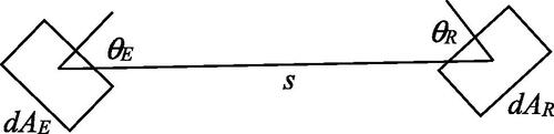
View factors are a fundamental property for calculating diffuse radiation transfer between two surfaces. A view factor between two surfaces represents the proportion of radiation leaving an emitting surface and incident to a receiving surface compared to the total radiation leaving the emitting surface. Figure 1 shows the important properties required to evaluate the view factor from a differential area, dA_E to a receiving differential area, dA_R. The view factor is given as [1]: (1) $${dF}_{E,R}=\frac{\cos \hspace{0.17em}{\theta }_E\cos \hspace{0.17em}{\theta }_R}{\pi \mathrm{ }{S}^2}d{A}_R$$(1)

Figure 1. View factor between differential areas.

For two finite areas the view factor is calculated by integrating (1(1) $${dF}_{E,R}=\frac{\cos \hspace{0.17em}{\theta }_E\cos \hspace{0.17em}{\theta }_R}{\pi \mathrm{ }{S}^2}d{A}_R$$(1) ) across the emitting and receiving areas. (2) $$F_{E,R}=\frac{1}{A_E}{\int }_{A_E}^{\mathrm{ }}{\int }_{A_R}^{\mathrm{ }}\frac{\cos \hspace{0.17em}{\theta }_E\cos \hspace{0.17em}{\theta }_R}{\pi \mathrm{ }{S}^2}d{A}_R\mathrm{ }d{A}_E$$(2)

There are many different techniques for evaluating (2(2) $$F_{E,R}=\frac{1}{A_E}{\int }_{A_E}^{\mathrm{ }}{\int }_{A_R}^{\mathrm{ }}\frac{\cos \hspace{0.17em}{\theta }_E\cos \hspace{0.17em}{\theta }_R}{\pi \mathrm{ }{S}^2}d{A}_R\mathrm{ }d{A}_E$$(2) ), some of which are discussed further below. This article is the third in a series discussing the merits of a hybrid Monte-Carlo method for evaluating view factors [2,3]. The novelty of the work is that for the most part the use of ray tracing for calculating view factors is restricted to view factor configurations where the two surfaces have a common edge or point. Even for these view factor configurations the use of ray tracing is minimized. In [2] an approach for evaluating view factor configurations is one based on applying a Monte-Carlo method to (2(2) $$F_{E,R}=\frac{1}{A_E}{\int }_{A_E}^{\mathrm{ }}{\int }_{A_R}^{\mathrm{ }}\frac{\cos \hspace{0.17em}{\theta }_E\cos \hspace{0.17em}{\theta }_R}{\pi \mathrm{ }{S}^2}d{A}_R\mathrm{ }d{A}_E$$(2) ) directly. This works well except for view factor configurations with a common edge. For these scenarios a hybrid method is found to work well, where for an area near the common edge, ray tracing is applied, and the numerical integration technique is applied remote from the common edge. In [3] the work is extended to look at different view factor configurations and provide a more in-depth characterization of the hybrid Monte-Carlo method. This article looks at how best to apply the hybrid Monte-Carlo method to view factor systems rather than individual view factor configurations.

2. Literature review

In the open literature there are several reviews of different methods for evaluating view factors [4,5]. For certain view factor configurations, the 4-dimensional integral, (2(2) $$F_{E,R}=\frac{1}{A_E}{\int }_{A_E}^{\mathrm{ }}{\int }_{A_R}^{\mathrm{ }}\frac{\cos \hspace{0.17em}{\theta }_E\cos \hspace{0.17em}{\theta }_R}{\pi \mathrm{ }{S}^2}d{A}_R\mathrm{ }d{A}_E$$(2) ) can be converted to 2-dimensional line integrals using Stokes’ theorem [6]. The line integrals can then be solved using a deterministic numerical quadrature scheme [7].

The most common numerical technique for evaluating view factors is the Monte-Carlo method combined with ray tracing [8–17]. A large number of references are cited as ray tracing is ubiquitous in the use of the Monte-Carlo method for numerically calculating view factors. The Monte-Carlo method is generally the method of choice as it is flexible and can be applied to many view factor configurations. The disadvantage of the Monte-Carlo method is it is a stochastic technique, and the central limit theorem applies. A corollary to the central limit theorem is a convergence result, (3) $$\left|F_{E,R}-\widetilde{F_{E,R}}\right|<A{N}_{\mathit{ray}}^{-0.5}$$(3) where the over bar indicates an approximate value for the view factor calculated using the Monte-Carlo method and A is a constant. The power law index n = –0.5 is a slow rate of convergence compared to many deterministic numerical methods.

The Monte-Carlo method can be subdivided into one based on a finite element representation of the domain [10,13] or one based on surfaces represented by composites of primitive shapes [2,3,14]. In the primitive shape approach the domain is represented by a combination of geometric shapes such as cylinders, rectangles, disks, and pipe bends. It is the primitive shape implementation of the Monte-Carlo method considered here.

In this article we consider three variants of the Monte-Carlo method, labeled for convenience as MC_RT, MC_NI and MC_H. These labels refer to the Monte-Carlo method with ray tracing, the Monte-Carlo method applied directly to the numerical integration of the view factor integral, (2(2) $$F_{E,R}=\frac{1}{A_E}{\int }_{A_E}^{\mathrm{ }}{\int }_{A_R}^{\mathrm{ }}\frac{\cos \hspace{0.17em}{\theta }_E\cos \hspace{0.17em}{\theta }_R}{\pi \mathrm{ }{S}^2}d{A}_R\mathrm{ }d{A}_E$$(2) ) and a hybrid Monte-Carlo method that is a combination of the other two. Details of the respective Monte-Carlo methods are given in the following section as well as a summary of the different methods is stated in Table 1.

Table 1. A summary of the different Monte-Calo methods and quasi-Monte-Carlo methods.

Method—label	Main points of method
MC_RT	Standard Monte-Carlo method based on ray tracing and pseudo-random numbers
QM_RT	Quasi-Monte-Carlo method using ray tracing and quasi-random numbers generated using Sobol sequences
MC_NI	Monte-Carlo method using the approximation (12(12) $$\widetilde{F_{E,R}}=\frac{A_R\mathrm{ }}{N_{\mathit{fun}}}\sum _{i=1}^{N_{\mathit{fun}}}{F}_i$$(12) )
QM_NI	Quasi-Monte-Carlo method using (12(12) $$\widetilde{F_{E,R}}=\frac{A_R\mathrm{ }}{N_{\mathit{fun}}}\sum _{i=1}^{N_{\mathit{fun}}}{F}_i$$(12) ) and quasi-random numbers generated using Sobol sequences
MC_H	Monte-Carlo method using a combination of MC_RT and MC_NI for view factor configurations with a common edge/ point between emitting and receiving surface. Note for a view factor system with any view factor configuration with a common edge MC_H is used. All other view factor configurations within the system are solved using MC_NI. For the system the method is described as MC_H.
QM_H	Similar to MC_H except quasi-random numbers generated using Sobol sequences are used as part of the method in place of pseudo-random numbers.

The relatively slow convergence rate of the Monte-Carlo method has motivated much research into many different potential improvements to the original Monte-Carlo method. For example, using quasi-random numbers that are space filling rather than pseudo random numbers can give a much-improved convergence rate. In this context a space filling sequence is one where the next value in the sequence cannot be predicted and is not close to previous values in the sequence. In this way the clustering of values is avoided. This is not truly random, and therefore the central limit theorem does not apply. For numerical integration on the unit hypercube, provided the integral kernel is sufficiently smooth the convergence rate of a quasi-Monte-Carlo method is given by the Koksma–Hlawka inequality [18]. (4) $$\left|I-I_n\right|\le A\frac{{\left(\ln \hspace{0.17em}n\right)}^s}{n}$$(4)

For some constant, A and s is the dimension of the hypercube, where I_n is the approximate integral value. The quasi-random number sequences are called low discrepancy sequencies [18]. There are a number of candidate space filling low discrepancy sequences available such as Sobol sequences [19,20] and Halton sequences [21]. The different low discrepancy sequences differ in the algorithm used to generate the quasi-random numbers. Halton sequences and Sobol sequences are investigated in [2] in the context of evaluating view factors. A conclusion of [2] is both types of sequence deliver a similar level of accuracy, but Sobol sequences are favored as they are marginally more efficient to generate. More details of Sobol sequences in the context of view factors are given in [2].

We consider three variants of the quasi-Monte-Carlo method, labeled for convenience as QM_RT, QM_NI and QM_H. These labels refer to the quasi-Monte-Carlo method with ray tracing, the quasi-Monte-Carlo method applied directly to the numerical integration of the view factor integral, (2(2) $$F_{E,R}=\frac{1}{A_E}{\int }_{A_E}^{\mathrm{ }}{\int }_{A_R}^{\mathrm{ }}\frac{\cos \hspace{0.17em}{\theta }_E\cos \hspace{0.17em}{\theta }_R}{\pi \mathrm{ }{S}^2}d{A}_R\mathrm{ }d{A}_E$$(2) ) and a hybrid quasi-Monte-Carlo method that is a combination of the other two. Details of the respective quasi-Monte-Carlo methods are given in the following section as well as a summary of the different methods is stated in Table 1.

In radiating systems with many surfaces, typical of the finite element Monte-Carlo method, significant improvements in efficiency for ray tracing is achieved by partitioning the domain and by so doing reducing the application of the ray tracing intersection test to a subset of the possible surfaces in the system [22–24]. View factor smoothing is another approach to improve efficiency [25–27], although the benefits of such approaches has been questioned [28].

Recently the Monte-Carlo method with ray tracing (MC_RT) and the quasi-Monte-Carlo method with ray tracing (QM_RT) as the methods of choice was questioned [2]. In [2] rather than tracing rays the Monte-Carlo method and Quasi-Monte-Carlo method is applied directly to (2(2) $$F_{E,R}=\frac{1}{A_E}{\int }_{A_E}^{\mathrm{ }}{\int }_{A_R}^{\mathrm{ }}\frac{\cos \hspace{0.17em}{\theta }_E\cos \hspace{0.17em}{\theta }_R}{\pi \mathrm{ }{S}^2}d{A}_R\mathrm{ }d{A}_E$$(2) ). In 3-dimensions this replaces the ray trace calculations with a number of vector operations. These approaches are the Monte-Carlo method, MC_NI and quasi-Monte-Carlo method, QM_NI. The NI identifying the method as one using numerical integration of (2(2) $$F_{E,R}=\frac{1}{A_E}{\int }_{A_E}^{\mathrm{ }}{\int }_{A_R}^{\mathrm{ }}\frac{\cos \hspace{0.17em}{\theta }_E\cos \hspace{0.17em}{\theta }_R}{\pi \mathrm{ }{S}^2}d{A}_R\mathrm{ }d{A}_E$$(2) ) rather than ray tracing. Provided the two surfaces are not touching or very close to each other the use of Monte-Carlo numerical integration is more efficient than ray tracing [2]. Each function evaluation requires less run-time than a ray trace and unless the two surfaces are very close together fewer function evaluations are required to achieve a given numerical accuracy [3]. For view factors with a common edge or point a hybrid Monte-Carlo method, (MC_H) and a hybrid quasi-Monte-Carlo method, (QM_H) are proposed in [2] that are a combination of numerical integration and ray tracing. Further characterization of the hybrid Monte-Carlo method is given in [3]. A summary of the important differences between the different Monte-Carlo methods and quasi-Monte-Carlo methods is summarized in Table 1.

In this article the work on the hybrid Monte-Carlo method is extended to look at its application to view factor systems rather than individual view factor configurations. View factor systems require a different implementation of MC_H than for individual view factor configurations. In this article how best to use view factor algebra is considered. This is relatively straightforward although has advantages over the application of view factor algebra to the Monte-Carlo method combined with ray tracing. Of more interest and is novel is the error analysis for nonuniform allocation of function evaluations to different view factors. More details of this are given below.

3. The Monte-Carlo method

The Monte-Carlo method is used to simulate many different physical processes that have a basis in high-dimensional problems, examples being the simulation of turbulence–radiation interaction [29–32]. The Monte-Carlo method is also used to solve the pdf transport model [33,34], which has the potential to model turbulence–chemistry interactions in turbulent combusting flows [35,36]. We will restrict attention to the calculation of view factor configurations and view factor systems using the Monte-Carlo method and quasi-Monte-Carlo method.

3.1. The Monte-Carlo method combined with ray tracing (MC_RT)

In the Monte-Carlo method applied to the evaluation of view factors using ray tracing is the equivalent of recasting the view factor integral to an equivalent representation. (5) $$F_{E,R}=\frac{1}{A_{E}2\pi }{\int }_{A_E}^{\mathrm{ }}{\int }_0^{2\pi }{\int }_0^{\raisebox{1ex}{$\pi $}\!\left/ \!\raisebox{-1ex}{$2$}\right.}\overline{F}\left(x_E,\theta ,\phi \right)\sin \hspace{0.17em}\theta \mathrm{ }d\theta \mathrm{ }d\phi \mathrm{ }d{A}_E$$(5) $$\overline{F}=\{\begin{array}{l}1 \text{ray intersects surface} R\\ 0 \mathrm{otherwise} \end{array}$$ x_E is the point vector on the emitting surface, θ and φ are spherical coordinates determining the ray orientation. Each ray traced requires four pseudo-random numbers or quasi-random numbers.

The view factor is approximated as, (6) $$\widetilde{F_{E,R}}=\frac{N_{\mathit{ray}\mathrm{ }E,R}\mathrm{ }}{N_{\mathit{ray},E}}$$(6) where N_ray,E is the total number of rays originating from surface E and N_{ray E,R} is the number of rays originating from surface E that intersect surface R.

When considering MC_RT applied to a system of view factors rather than a single view factor configuration, the method is much the same as described above except rays for each emitting surface are traced to the closest surface they intersect. As all rays must intersect a surface this means that the energy conservation view factor algebra rule is satisfied, (7) $$\sum _{j=1}^{N_{\mathit{surf}}}{F}_{i,j}=1$$(7)

The other two view factor rules, are the equal exchange area rule, (8) $$A_i{F}_{i,j}=A_j{F}_{j,i}$$(8) and the view factor additive rule, (9) $$F_{i,j+k}=F_{i,j}+F_{i,k}$$(9) are only satisfied in the limit of an infinite number of rays traced. It is this version of the Monte-Carlo method combined with ray tracing, MC_RT that is applied to view factor systems and used as a reference for comparison with other implementations of the Monte-Carlo method.

In [25], it is proposed to modify MC_RT to satisfy the three view factor algebra rules. Ray tracing is used to calculate half the off-diagonal view factors. The remaining off-diagonal view factors are calculated using the equal exchange area rule (8(8) $$A_i{F}_{i,j}=A_j{F}_{j,i}$$(8) ). The diagonal view factors are calculated using (7(7) $$\sum _{j=1}^{N_{\mathit{surf}}}{F}_{i,j}=1$$(7) ). There are two problems with this approach; all rays are traced and approximately half the rays traced are used in the calculation of view factors and using view factor algebra it is possible to calculate view factors that are outside the unit interval. Limiters on the calculated view factors can be imposed but then the rules of view factor algebra are no longer satisfied.

3.2. The hybrid Monte-Carlo method (MC_H)

The hybrid Monte Carlo method where possible avoids ray tracing as it is a computationally expensive procedure compared to the use of numerical integration. In the first instance the calculation of view factors with no common edge or corner are considered. This is the MC_NI Monte-Carlo method. 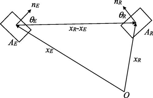The basis of the approach is to replace the kernel of integral (2(2) $$F_{E,R}=\frac{1}{A_E}{\int }_{A_E}^{\mathrm{ }}{\int }_{A_R}^{\mathrm{ }}\frac{\cos \hspace{0.17em}{\theta }_E\cos \hspace{0.17em}{\theta }_R}{\pi \mathrm{ }{S}^2}d{A}_R\mathrm{ }d{A}_E$$(2) ) with several vector operations; see Figure 2 for the definition of the vectors, connecting points on the emitting surface to points on the receiving surface. (10) $$F_{E,R}=\frac{1}{A_E}{\int }_{A_E}^{\mathrm{ }}{\int }_{A_R}^{\mathrm{ }}\frac{-\left(x_E-x_R\right).n_E\mathrm{ }\left(x_E-x_R\right).n_R}{\pi {\left(\left(x_E-x_R\right).\mathrm{ }\left(x_E-x_R\right)\right)}^2}d{A}_R\mathrm{ }d{A}_E$$(10)

Figure 2. Vectors used in the formulation of the view factor expression (10)(10) $$F_{E,R}=\frac{1}{A_E}{\int }_{A_E}^{\mathrm{ }}{\int }_{A_R}^{\mathrm{ }}\frac{-\left(x_E-x_R\right).n_E\mathrm{ }\left(x_E-x_R\right).n_R}{\pi {\left(\left(x_E-x_R\right).\mathrm{ }\left(x_E-x_R\right)\right)}^2}d{A}_R\mathrm{ }d{A}_E$$(10) .

Applying the Monte-Carlo method to evaluate (10(10) $$F_{E,R}=\frac{1}{A_E}{\int }_{A_E}^{\mathrm{ }}{\int }_{A_R}^{\mathrm{ }}\frac{-\left(x_E-x_R\right).n_E\mathrm{ }\left(x_E-x_R\right).n_R}{\pi {\left(\left(x_E-x_R\right).\mathrm{ }\left(x_E-x_R\right)\right)}^2}d{A}_R\mathrm{ }d{A}_E$$(10) ), four pseudo random numbers are used to calculate a point on the emitting surface and a point on the receiving surface. (11) $$x_E=f_E\left({Ra}_1,\mathrm{ }{Ra}_2\right) \mathrm{and}\mathrm{ }{x}_R=f_R\left({Ra}_3,\mathrm{ }{Ra}_4\right)$$(11) where f_E and f_R represent the manifolds of the emitting and receiving surfaces. The normal unit vectors for the two surfaces, n_E and n_R are calculated based on x_E and x_R and the prescribed primitive shape. Let the evaluation of the kernel of (10(10) $$F_{E,R}=\frac{1}{A_E}{\int }_{A_E}^{\mathrm{ }}{\int }_{A_R}^{\mathrm{ }}\frac{-\left(x_E-x_R\right).n_E\mathrm{ }\left(x_E-x_R\right).n_R}{\pi {\left(\left(x_E-x_R\right).\mathrm{ }\left(x_E-x_R\right)\right)}^2}d{A}_R\mathrm{ }d{A}_E$$(10) ) be denoted F_i where the subscript indicates the sequence of function evaluations of the kernel. The approximation to the view factor is given as: (12) $$\widetilde{F_{E,R}}=\frac{A_R\mathrm{ }}{N_{\mathit{fun}}}\sum _{i=1}^{N_{\mathit{fun}}}{F}_i$$(12)

As we will see below the above algorithm has a very different numerical behavior than applying ray tracing. Each function evaluation requires less run-time than tracing a ray. For most view factor configurations with no common edge fewer function evaluations are required to achieve a given accuracy compared to ray tracing. The exception to this is if the two surfaces are very close together. For two coaxial unit-squares the crossover in efficiency between evaluating (10(10) $$F_{E,R}=\frac{1}{A_E}{\int }_{A_E}^{\mathrm{ }}{\int }_{A_R}^{\mathrm{ }}\frac{-\left(x_E-x_R\right).n_E\mathrm{ }\left(x_E-x_R\right).n_R}{\pi {\left(\left(x_E-x_R\right).\mathrm{ }\left(x_E-x_R\right)\right)}^2}d{A}_R\mathrm{ }d{A}_E$$(10) ) compared to ray tracing is in the interval. (13) $$0.2\le \frac{z}{L}\le 0.5$$(13) where z is the distance between the two squares and L is the length of the side of the squares [3]. Note the crossover point in efficiency favors the method based on (10(10) $$F_{E,R}=\frac{1}{A_E}{\int }_{A_E}^{\mathrm{ }}{\int }_{A_R}^{\mathrm{ }}\frac{-\left(x_E-x_R\right).n_E\mathrm{ }\left(x_E-x_R\right).n_R}{\pi {\left(\left(x_E-x_R\right).\mathrm{ }\left(x_E-x_R\right)\right)}^2}d{A}_R\mathrm{ }d{A}_E$$(10) ) even more when the computer run-time of evaluating (12(12) $$\widetilde{F_{E,R}}=\frac{A_R\mathrm{ }}{N_{\mathit{fun}}}\sum _{i=1}^{N_{\mathit{fun}}}{F}_i$$(12) ) compared to ray tracing is factored into the analysis.

For view factors with a common edge or corner it is possible for the distance between the emitting and receiving point to be very small or even zero. There is a singularity in (2(2) $$F_{E,R}=\frac{1}{A_E}{\int }_{A_E}^{\mathrm{ }}{\int }_{A_R}^{\mathrm{ }}\frac{\cos \hspace{0.17em}{\theta }_E\cos \hspace{0.17em}{\theta }_R}{\pi \mathrm{ }{S}^2}d{A}_R\mathrm{ }d{A}_E$$(2) ) and (10(10) $$F_{E,R}=\frac{1}{A_E}{\int }_{A_E}^{\mathrm{ }}{\int }_{A_R}^{\mathrm{ }}\frac{-\left(x_E-x_R\right).n_E\mathrm{ }\left(x_E-x_R\right).n_R}{\pi {\left(\left(x_E-x_R\right).\mathrm{ }\left(x_E-x_R\right)\right)}^2}d{A}_R\mathrm{ }d{A}_E$$(10) ).

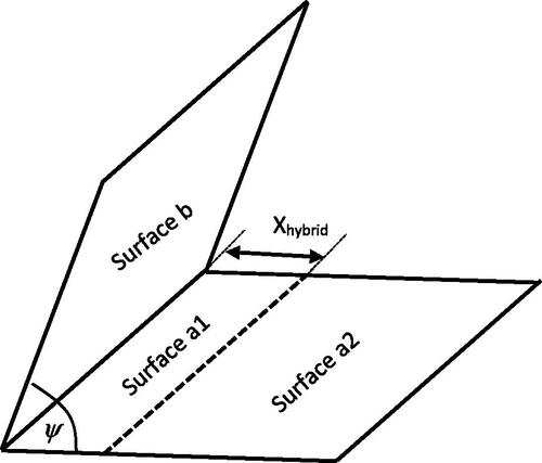
The solution to this is to take a hybrid approach, near the common edge ray tracing is applied and further away from the common edge the numerical integration approach based on (10(10) $$F_{E,R}=\frac{1}{A_E}{\int }_{A_E}^{\mathrm{ }}{\int }_{A_R}^{\mathrm{ }}\frac{-\left(x_E-x_R\right).n_E\mathrm{ }\left(x_E-x_R\right).n_R}{\pi {\left(\left(x_E-x_R\right).\mathrm{ }\left(x_E-x_R\right)\right)}^2}d{A}_R\mathrm{ }d{A}_E$$(10) ) is applied, see Figure 3. Consider the view factor F_a–b for the configuration shown in Figure 3. The area of the emitting surface is subdivided into two areas. Let the area adjacent to the common edge be denoted, A_a1 and the remaining area be A_a2. For the area A_a1 ray tracing is applied, for the other part of the emitting surface numerical integration of (10(10) $$F_{E,R}=\frac{1}{A_E}{\int }_{A_E}^{\mathrm{ }}{\int }_{A_R}^{\mathrm{ }}\frac{-\left(x_E-x_R\right).n_E\mathrm{ }\left(x_E-x_R\right).n_R}{\pi {\left(\left(x_E-x_R\right).\mathrm{ }\left(x_E-x_R\right)\right)}^2}d{A}_R\mathrm{ }d{A}_E$$(10) ) is applied. The view factor for the total emitting area is then recovered using view factor algebra.

Figure 3. The partition of the emitting surface for a view factor configuration with a common edge.

Given the number of rays/function evaluations allocated to evaluate the view factor, F_a–b is N_total then the number of rays or function evaluation for the view factor calculations, F_a1–b, and F_a2–b, can be based on the areas, A_a1 and A_a2, (14) $$N_{\mathit{ray},a1}=\frac{A_{a1}}{A_{a1}+A_{a2}}{N}_{\mathit{total}}$$(14) (15) $$N_{\mathit{fun},a2}=\frac{A_{a2}}{A_{a1}+A_{a2}}{N}_{\mathit{total}}$$(15)

The view factor, F_a–b can then be calculated using the equal exchange area rule and the addition property of view factors. (16) $$F_{b-a}=F_{b-a1+a2}=\frac{A_{a1}}{A_b}{F}_{a1-b}+\frac{A_{a2}}{A_b}{F}_{a2\text{-}b}$$(16) (17) $$F_{a-b}=\frac{A_b}{A_a}{F}_{b-a}$$(17)

The hybrid method is easily extended to view factor configurations with a common corner [3]. The separation of the emitting surface into two areas is partitioned on the basis of the length X_hybrid, see Figure 3. In [3] it is found that the key parameter for determining the optimal value for X_hybrid depends on the angle, ψ between the two surfaces. In [3] two correlations for X_hybrid are proposed that demonstrate a degree of universality, one for the Monte-Carlo method, MC_H and one for the quasi-Monte-Carlo method, QM_H. (18) $$\begin{array}{c}\begin{array}{c}{X}_{\mathit{hybrid},MC}=0.057{\psi }^2-0.347\psi +0.5407\\ \frac{\pi }{6}\le \psi \le \pi \end{array}\\ X_{\mathit{hybrid},QM}=\max \left\{0,\mathrm{ }-0.1165\psi +0.3609\right\}\end{array}$$(18)

A summary of the differences between the respective Monte-Carlo methods and quasi-Monte-Carlo methods is given in Table 1.

4. View factor configurations

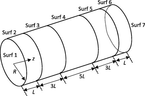
The calculation of a view factor system considered below is given in Figure 4. This is a test problem used to evaluate different Monte-Carlo methods in [26,37]. Before we consider the view factor system it is of interest to consider the application of the Monte-Carlo method to two view factor configurations related to the view factor system test problem.

Figure 4. Test view factor system.

The calculation of the view factor for the internal surfaces of two coaxial cylinders, VF_CYL and the view factor of two coaxial disks, VF_DISK. The view factor configurations are shown in Figure 5. These view factor configurations are given in [38].

Figure 5. View factor configurations: a) cylinder-to-cylinder and b) disk-to-disk.

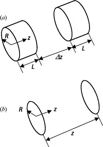
4.1. View factor configuration VF_CYL

For this view factor configuration, the radius of the cylindrical shells is R = 1m and the height of each cylindrical shell is L = 1m. The view factor for four different separation distances between the cylindrical shells, Δz = 0, 1, 5 and 10m are calculated using six Monte-Carlo methods, MC_RT, QM_RT, MC_NI, QM_NI, MC_H and QM_H.

As discussed in [2,3] the computational run-time for tracing a ray is more than the evaluation of a single function evaluation of the integral kernel defined in (10(10) $$F_{E,R}=\frac{1}{A_E}{\int }_{A_E}^{\mathrm{ }}{\int }_{A_R}^{\mathrm{ }}\frac{-\left(x_E-x_R\right).n_E\mathrm{ }\left(x_E-x_R\right).n_R}{\pi {\left(\left(x_E-x_R\right).\mathrm{ }\left(x_E-x_R\right)\right)}^2}d{A}_R\mathrm{ }d{A}_E$$(10) ). To allow a consistent evaluation of the relative error vs. computational cost the run-time for the evaluation of the integral kernel of (10(10) $$F_{E,R}=\frac{1}{A_E}{\int }_{A_E}^{\mathrm{ }}{\int }_{A_R}^{\mathrm{ }}\frac{-\left(x_E-x_R\right).n_E\mathrm{ }\left(x_E-x_R\right).n_R}{\pi {\left(\left(x_E-x_R\right).\mathrm{ }\left(x_E-x_R\right)\right)}^2}d{A}_R\mathrm{ }d{A}_E$$(10) ) and ray tracing operations can be used to define a relative run-time for a Monte-Carlo method or quasi-Monte-Carlo method, relative to MC_RT as, (19) $$t_{\mathit{rel},M\mathrm{C}\_H}=\frac{t_{MC\_H}}{t_{MC\_RT}}$$(19) where t_{MC_RT} is the time required to trace 1,000 rays and t_{MC_H} is the time to evaluate 1,000 rays/function evaluations depending on the view factor configuration. The sensitivity of t_{rel,MC_H} to the exact number of rays traced was investigated and found to be insensitive. The relative run-time for MC_NI, QM_NI, QM_RT and QM_H are defined in the same way. Note the relative run-time for QM_RT is slightly less than one, see Table 2, this is because the time required to generate the Sobol sequence is slightly less than the equivalent time to generate the same number of pseudo-random numbers used in MC_RT.

Table 2. VF_CYL, computational effort to achieve 1% relative error.

Method	Δz	Nray	Nfun	trel	Nray,eff
MC_RT	0	20,000	–	1	20,000
MC_RT	10	6.3 × 10^7*	–	1	6.3 × 10^7
QM_RT	0	3,900	–	0.97	3,800
QM_RT	10	1.2 × 10^7*	–	0.97	1.2 × 10^7
MC_H	0	–	4,500	0.532	2,400
MC_NI	10	–	4,900	0.532	2,600
QM_H	0	–	620	0.542	340
QM_NI	10	–	660	0.542	360

* Estimated from power law curve fit.

Introducing the relative run times enable the calculation of an effective number of rays, N_ray,eff. (20) $$N_{\mathit{ray},\mathit{eff},MC\_H}=N_{\mathit{fun}}\mathrm{ }{t}_{\mathit{rel},MC\_H}$$(20)

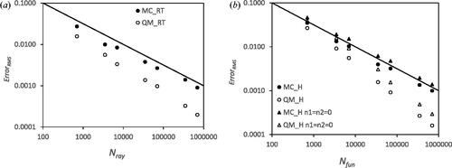
For the four different Monte-Carlo methods the relative error in the view factor is shown in Figure 6. The relative error curves are calculated using 100 sample averages factoring out stochastic effects and making it easier to identify trends as the number of rays, N_ray or effective number of rays, N_ray,eff increases. For Figure 6b–d the relative error is plotted against N_ray,eff. The relative error curve is plotted on log–log axis such that a straight line indicates a power law relationship. To demonstrate that the Monte-Carlo methods satisfy the central limit theorem A line with a power law index of n = –0.5 is also plotted.

Figure 6. Relative error of the cylinder-to-cylinder view factor configuration calculated using: a) MC_RT, b) QM_RT c) MC_H/MC_NI, and d) QM_H/QM_NI.

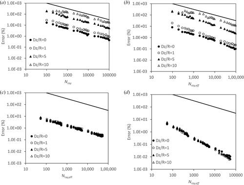
In Figure 6a the relative error curves calculated using MC_RT are shown. The curves as expected follow a power law curve with a power law index of n = –0.5. As the separation distance between the two cylindrical shells increases the relative error increases. This again is typical behavior of the Monte-Carlo method combined with ray tracing. Considering the relative error curves calculated using QM_RT, shown in Figure 6b. For the same number of rays, and separation distance, the QM_RT method gives a lower relative error than MC_RT and the curves are close to a power law curve, but the index is higher than for a standard Monte-Carlo method. For Δz = 1m the power law index is n = –0.64. The improvement in performance will be considered further below.

Figure 6c shows the relative error calculated using MC_H/MC_NI. For Δz = 0 the two cylindrical shells are touching, and the hybrid Monte-Carlo method is appropriate. For Δz > 0 the Monte-Carlo method applied is MC_NI. Comparing this set of results with MC_RT in Figure 6a, we see that the relative error decreases with an approximate power law index of n = –0.5, but the relative error is insensitive to the separation distance, Δz. This is significant as this is the opposite behavior of Monte-Carlo methods based on ray tracing. Further a close inspection of Figure 6a and Figure 6c we see that for all separation distances the method MC_NI/MC_H is superior to MC_RT with the difference in relative error growing with separation distance. The relative error for the method, QM_NI/QM_H is shown in Figure 6d. Again, for Δz = 0 the method applied is the hybrid version of the quasi-Monte-Carlo method, QM_H. For Δz > 0 the quasi-Monte-Carlo method applied is QM_NI. A conclusion from comparing Figure 6b, QM_RT and Figure 6d, QM_H/QM_NI is that the sensitivity of the relative error to separation distance is not present in the QM_H/QM_NI error curves. The power law index for the relative error for QM_NI, Δz = 1, is n = –0.95.

To give a clearer picture of the respective performance of the different Monte-Carlo methods it is worthwhile to focus on the computational run-time to achieve a given accuracy. The number of rays and number of function evaluations to achieve a relative error of 1% for the different separation distances and different Monte-Carlo methods is given in Table 2. Note where a method has not calculated a relative error of 1% i.e. more rays are required then an estimate of the required number of rays is calculated from the power law curve fit. Data for two separation distances, Δz = 0 and 10m are given in Table 2. From the table, it can be concluded that the reduction in computational run-time using MC_NI/MC_H and QM_NI/QM_H is significant.

Using the relative run-time defined in (19(19) $$t_{\mathit{rel},M\mathrm{C}\_H}=\frac{t_{MC\_H}}{t_{MC\_RT}}$$(19) ) and the parameter N_ray,eff, (20(20) $$N_{\mathit{ray},\mathit{eff},MC\_H}=N_{\mathit{fun}}\mathrm{ }{t}_{\mathit{rel},MC\_H}$$(20) ), a direct comparison of computational cost to achieve an accuracy of 1% is possible. The speed-up parameter, S_p, for MC_H, relative to MC_RT is defined as: (21) $$S_{p,MC\_H}=\frac{N_{\mathit{ray},M{C}_{RT},1\mathrm{\%}}\mathrm{ }}{N_{\mathit{ray},\mathit{eff}\mathrm{ }MC\_H,1\mathrm{\%}}}$$(21)

The speed-up parameter for other Monte-Carlo methods and quasi-Monte-Carlo methods can be defined similarly. A conclusion that can be inferred from the data in Table 2 is the computational run-time is significantly lower using a hybrid Monte-Carlo method or one based on direct integration of (10(10) $$F_{E,R}=\frac{1}{A_E}{\int }_{A_E}^{\mathrm{ }}{\int }_{A_R}^{\mathrm{ }}\frac{-\left(x_E-x_R\right).n_E\mathrm{ }\left(x_E-x_R\right).n_R}{\pi {\left(\left(x_E-x_R\right).\mathrm{ }\left(x_E-x_R\right)\right)}^2}d{A}_R\mathrm{ }d{A}_E$$(10) ) than one based purely on ray tracing. For Δz = 0m, for a 1% relative error, MC_H has a speed-up of S_{p,MC_H} = 8.3 compared to MC_RT and QM_H has a speed-up of S_{p,QM_H} = 59.

For Δz = 10m, the results are even more favorable for Monte-Carlo methods with no ray tracing. For a 1% relative error, MC_NI has a speed-up of S_{p,MC_H} = 24,000 compared to MC_RT and QM_NI has a speed-up of 180,000. This is really a statement of how MC_RT and QM_RT perform poorly for surfaces remote from each other. This occurs as when the distance between the emitting and receiving surface is large the total number of rays required to have a reasonable sample of rays incident on the receiving surface must be large. For the Monte-Carlo methods based on numerical integration, MC_NI and QM_NI these have a very different numerical behavior. If the distance between the emitting and receiving surface is large, then the integral kernel in (10(10) $$F_{E,R}=\frac{1}{A_E}{\int }_{A_E}^{\mathrm{ }}{\int }_{A_R}^{\mathrm{ }}\frac{-\left(x_E-x_R\right).n_E\mathrm{ }\left(x_E-x_R\right).n_R}{\pi {\left(\left(x_E-x_R\right).\mathrm{ }\left(x_E-x_R\right)\right)}^2}d{A}_R\mathrm{ }d{A}_E$$(10) ) approaches a constant function. For constant functions only one function evaluation is required. This is discussed further below for the next view factor configuration.

4.2. View factor configuration VF_DISK

In this subsection the disk-to-disk view factor configuration is considered, see Figure 5b. For this configuration 4 separation distances are specified, z = 1, 2, 5 and 10 m. The relative error curves shown in Figure 7 are generated using the same methodology with 100 samples calculated for each data point in the figure to give a smooth average relative error.

Figure 7. Relative error of the disk-to-disk view factor configuration calculated using: a) MC_RT, b) QM_RT c) MC_NI, d) and QM_NI.

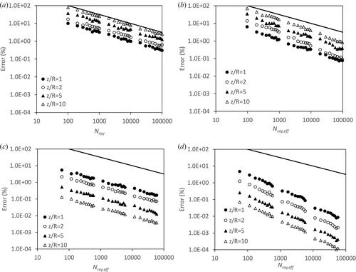
The MC_RT and QM_RT relative error are shown in Figure 7a and Figure 7b, respectively. The analysis of the figures is similar to Figure 6a and Figure 6b for the view factor configuration VF_CYL and will not be repeated in any detail, suffice it to say the two methods behavior is similar for both view factor configurations. Applying a power law trend line to the relative error calculated using QM_RT gives a power law index of n = –0.75.

Considering the relative error calculated using MC_NI and QM_NI, see Figure 7c and Figure 7d, respectively the relative error curves are somewhat different to that exhibited for VF_CYL, see Figure 6c and Figure 6d. In Figure 7c and Figure 7d, the relative error curves are sensitive to the separation distance between the disks in VF_DISK. For the VF_CYL configuration there is little sensitivity of the relative error to the separation distance, Δz, see Figure 6c and Figure 6d. For the VF_DISK configuration as the separation distance increases the relative error is dramatically reduced. This is the opposite way round compared to the Monte-Carlo methods based on ray tracing. Fitting a power law trend line on the disk-to-disk relative errors for QM_NI gives a power law index of n = –0.96.

Similar to VF_CYL, Table 3 shows the computational effort to achieve a 1% error for the view factor configuration, VF_DISK. The data are calculated in the same way as for VF_CYL. Note the relative run-times in column, t_rel are different from Table 2. This is due to the ray intersection process being simpler for a disk-to-disk ray trace compared to a cylinder-to-cylinder ray trace. A cylinder-to-cylinder ray trace involves the solution of a quadratic equation. For z = 1m, for a 1% relative error, MC_NI has a speed-up of S_{p,MC_H} = 5.3 compared to MC_RT and QM_NI has a speed-up of 22. For z = 10m, the speed-up values for MC_NI and QM_NI are both 2.2 × 10⁵.

Table 3. VF_DISK, computational effort to achieve 1% relative error.

Method	z	Nray	Nfun	trel	Nray,eff
MC_RT	1	8,000	–	1	8,000
MC_RT	10	650,000*	–	1	650,000
QM_RT	1	1,400	–	0.97	1,400
QM_RT	10	68,000	–	0.97	66,000
MC_NI	1	–	2,600	0.590	1,500
MC_NI	10	–	5	0.590	3
QM_NI	1	–	650	0.572	370
QM_NI	10	–	5	0.572	3

* Estimated from power law curve fit.

Such large speed-up values are due to the very small number of function evaluations necessary to achieve a relative error of 1% for MC_NI and QM_NI. To appreciate why this might be we can define a parameter V_F, the variation in the integral kernel of (10(10) $$F_{E,R}=\frac{1}{A_E}{\int }_{A_E}^{\mathrm{ }}{\int }_{A_R}^{\mathrm{ }}\frac{-\left(x_E-x_R\right).n_E\mathrm{ }\left(x_E-x_R\right).n_R}{\pi {\left(\left(x_E-x_R\right).\mathrm{ }\left(x_E-x_R\right)\right)}^2}d{A}_R\mathrm{ }d{A}_E$$(10) ) as follows: (22) $$F(x_E,x_R)=\frac{-\left(x_E-x_R\right).n_E\mathrm{ }\left(x_E-x_R\right).n_R}{\pi {\left(\left(x_E-x_R\right).\mathrm{ }\left(x_E-x_R\right)\right)}^2}$$(22) (23) $$V_F=100\frac{F_{\max }-F_{\min }}{0.5\left(F_{\max }+F_{\min }\right)}$$(23)

An important point of note is that if V_F is zero then the kernel is a constant function. Constant functions require just one function evaluation to be exact. For the disk-to-disk view factor configuration, as the separation distance grows V_F tends to zero, requiring fewer and fewer function evaluations to achieve an accurate result.

5. View factors for a view factor system

Having assessed the different Monte-Carlo methods for two view factor configurations of relevance to the view factor system, see Figure 4, we can now move on to the calculation of the view factors for the system. For the view factor system, the view factors F_1–2 and F_7–6 have surfaces with a common edge, therefore, the evaluation of the Monte-Carlo method and quasi-Monte-Carlo method based on the numerical integration of (10(10) $$F_{E,R}=\frac{1}{A_E}{\int }_{A_E}^{\mathrm{ }}{\int }_{A_R}^{\mathrm{ }}\frac{-\left(x_E-x_R\right).n_E\mathrm{ }\left(x_E-x_R\right).n_R}{\pi {\left(\left(x_E-x_R\right).\mathrm{ }\left(x_E-x_R\right)\right)}^2}d{A}_R\mathrm{ }d{A}_E$$(10) ) are not considered in this section. For simplicity of discussion for view factor systems N_fun is used to denote the total number of “functions” used to evaluate a view factor where functions is placed in quotes as it is generalized to ray tracing and function evaluations for the evaluation of F_1–2 and F_7–6 and other view factor surfaces with a common edge.

For MC_RT and QM_RT the extension of the ray tracing methodology to a view factor system is straightforward, each emitting surface is allocated a number of rays and when considering how the RMS error decays with rays traced the total number of rays traced for the system is considered. As well as confirming the average RMS error curve has a power law index of n = –0.5 for MC_RT the results are compared with [26], and the average RMS curve presented here reproduces the average RMS error curve before view factor smoothing is applied in [26]. The average RMS error curves for MC_RT and QM_RT are compared with the hybrid Monte-Carlo method results below.

For the hybrid Monte-Carlo methods, MC_H and QM_H the situation is more complicated as there is some flexibility in the implementation. From the view factor configuration VF_DISK it is demonstrated that there is significant sensitivity of the relative error to the distance between the emitting and receiving surface. This is true for the ray trace methods also but to a lesser degree and there is no way of exploiting this as the surface a ray intersects is not known a priori. For the VF_CYL configuration and the Monte-Carlo methods, MC_H/MC_NI and QM_H/QM_NI there is less sensitivity of the relative error to the separation distance. When considering the average RMS error for a view factor system there is a sensitivity of the RMS error to the separation distance of the emitting and receiving surface. This will be explained below.

It is possible to investigate how varying the number of function evaluations allocated to each surface-to-surface calculation has an impact on the RMS error. We will consider pairs of view factors and triplet view factors with different allocations of function evaluations.

5.1. N_fun distribution for pairs of view factors

Consider the view factors F_1,2 and F_1,3. For these two view factors labeling X_1,2 as the proportion of function evaluations allocated to evaluate F_1,2, then, (24) $$X_{1,3}=1-X_{1,2}$$(24) (25) $$N_{1,2}=X_{1,2}{N}_{\mathit{fun},\mathit{total}}$$(25)

It is possible to systematically change X_1,2 and plot the RMS error for the two view factors. In Figure 8a the RMS Error/RMS Error_0.5 is plotted against X_1,2. Where RMS Error_0.5 represents the average RMS error using an equal distribution of function evaluations. The data is plotted in this way to quantify the improvement in performance relative to an equal allocation of function evaluations. The curves in Figure 8 are generated for X₁₂ = 0.02i, i = 1,2,…,49, spanning the unit interval. In all calculations N_fun,total is set to 1,000. The average RMS Error is calculated using N_sample = 1,000. A number of numerical experiments were completed to confirm that the location of the RMS error minimizer is insensitive to the value of N_fun,total used. Numerical experiments were also used to identify an appropriate value for N_sample.

Figure 8. Improvement in relative error for different values of X₁₂ for pairs of view factors, a) F₁₂, F₁₃ and b) F₁₂, F₁₇.

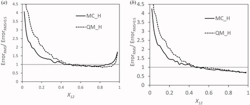
In Figure 8a, two curves are shown, the average RMS error calculated for MC_H and QM_H. The two curves have a similar shape that is well approximated to be a quartic polynomial. For values of X_1,2 above 0.5 the RMS error decreases to values below that for X_1,2 = 0.5. The minimizer values for M_H and QM_H are as follows: (26) $${\left(\begin{array}{c}{X}_{1,2}\\ X_{1,3}\end{array}\right)}_{\min ,MC\_H}=\left(\begin{array}{c}0.72\\ 0.28\end{array}\right)$$(26)

For this distribution of function evaluations: (27) $$\frac{\mathit{RMS}\mathrm{ }\mathit{Error}}{{\mathit{RMS}\mathrm{ }\mathit{Error}}_{0.5}}=0.89$$(27)

The equivalent data for the QM_H Monte-Carlo method are as follows: (28) $${\left(\begin{array}{c}{X}_{1,2}\\ X_{1,3}\end{array}\right)}_{\min ,QM\_H}=\left(\begin{array}{c}0.82\\ 0.18\end{array}\right)$$(28)

For this distribution of function evaluations: (29) $$\frac{\mathit{RMS}\mathrm{ }\mathit{Error}}{{\mathit{RMS}\mathrm{ }\mathit{Error}}_{0.5}}=0.83$$(29)

This is a marginal gain. It is to be expected that the improvement in RMS error would be small as Surface 2 and 3 are close to each other.

The above analysis is repeated for a number of pairs of view factors. We will only present one more view factor pair, F_1,2 and F_1,7. The RMS Error/RMS Error _0.5 vs. X_1,2 is shown in Figure 8b. For this pair of view factors there is no well-defined minimizing value. The minimum occurs at values approaching unity for X_1,2. The exact value calculated is more based on the small deviations due to the stochastic nature of the Monte-Carlo method. Of course, more samples in the average will reduce this but not to any real advantage. The minimizer values for X_1,2, X_1,7 together with the improvement in the RMS Error are given below. (30) $${\left(\begin{array}{c}{X}_{1,2}\\ X_{1,7}\end{array}\right)}_{\min ,MC\_H}=\left(\begin{array}{c}0.96\\ 0.04\end{array}\right)$$(30)

For this distribution of function evaluations: (31) $$\frac{\mathit{RMS}\mathrm{ }\mathit{Error}}{{\mathit{RMS}\mathrm{ }\mathit{Error}}_{0.5}}=0.71$$(31)

The equivalent data for the QM_H are as follows: (32) $${\left(\begin{array}{c}{\mathrm{X}}_{1,2}\\ X_{1,7}\end{array}\right)}_{\min ,QM\_H}=\left(\begin{array}{c}0.98\\ 0.02\end{array}\right)$$(32)

For this distribution of function evaluations: (33) $$\frac{\mathit{RMS}\mathrm{ }\mathit{Error}}{{\mathit{RMS}\mathrm{ }\mathit{Error}}_{0.5}}=0.69$$(33)

As expected with two receiving surfaces far from each other the improvement in RMS error is bigger when a nonuniform distribution of function evaluations are used. The gain in efficiency is still relatively small but should be viewed as a potential gain for only a small increase in algorithmic complexity, assuming some way of determining the matrix, $\left[X_{i,j}\right]$ without a priori knowledge of the view factor values. A further question is that as more view factors are introduced into the RMS error minimization does the gain in efficiency improve significantly?

5.2. Nfun distribution for view factor triplets

It is possible to extend the analysis to view factor triplets and investigate the potential improvement in the reduction of the average RMS Error. We will only present data for two sets of triplets, F_1,2, F_1,3 and F_1,4 and F_1,2, F_1,6 and F_1,7.

Figure 9a shows contour maps of the average RMS error for the triplet view factors, F_1,2, F_1,3 and F_1,4. There are 50 equally spaced contour values between zero and the maximum average RMS error calculated. The contour maps are generated from a 2D matrix of values for X_1,2 and X_1,3. (34) $$\begin{array}{l}\begin{array}{c}{X}_{1,2}=i\Delta X_{1,2}\\ X_{1,3}=j\Delta X_{1,3}\end{array}\\ X_{1,4}=1-X_{1,2}-X_{1,3}\end{array}$$(34)

Figure 9. Improvement in relative error for different values of X₁₂ and X₁₃ for view factor triplets, a) F₁₂, F₁₃, F₁₄ and b) F₁₂, F_16, F₁₇.

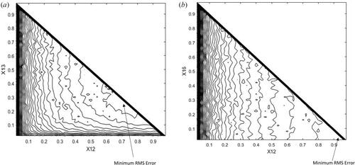
Note if X_1,4 is negative or zero then that combination of X_1,2, X_1,3 and X_1,4 is not possible, and the average RMS error is set to zero.

The matrix spacing is ΔX_1,2 = ΔX_1,3 = 0.02. Similar to the analysis for pairs of view factors the average RMS error is calculated using 1,000 samples and N_fun,total = 1,000. A range of values were explored for appropriate values of N_sample and N_fun,total to confirm that the RMS Error/RMS Error_0.33 minimum value and its location is insensitive to the values chosen. The minimization data are as follows, (35) $${\left(\begin{array}{c}{X}_{1,2}\\ X_{1,3}\\ X_{1,4}\end{array}\right)}_{\min ,MC\_H}=\left(\begin{array}{c}0.72\\ 0.2\\ 0.08\end{array}\right)$$(35) and $$\frac{\mathit{RMS}\mathrm{ }\mathit{Error}}{{\mathit{RMS}\mathrm{ }\mathit{Error}}_{0.33}}=0.76$$

For the QM_H Monte-Carlo method, (36) $${\left(\begin{array}{c}{X}_{1,2}\\ X_{1,3}\\ X_{1,4}\end{array}\right)}_{\min ,QM\_H}=\left(\begin{array}{c}0.78\\ 0.18\\ 0.04\end{array}\right)$$(36) and $$\frac{\mathit{RMS}\mathrm{ }\mathit{Error}}{{\mathit{RMS}\mathrm{ }\mathit{Error}}_{0.33}}=0.65$$

Figure 9b shows contour maps of the RMS error for the triplet view factors, F_1,2, F_1,6 and F_1,7. There are 50 equally spaced contour values between zero and the maximum average RMS error calculated on the matrix of points X_1,2, X_1,6. The contour map is calculated in the same way as the RMS error for the view factor triplet, F_1,2, F_1,3 and F_1,4. The minimization data for the view factor triplet F_1,2, F_1,6 and F_1,7, are as follows, (37) $${\left(\begin{array}{c}{X}_{1,2}\\ X_{1,6}\\ X_{1,7}\end{array}\right)}_{\min ,MC\_H}=\left(\begin{array}{c}0.92\\ 0.04\\ 0.04\end{array}\right)$$(37) and $$\frac{\mathit{RMS}\mathrm{ }\mathit{Error}}{{\mathit{RMS}\mathrm{ }\mathit{Error}}_{0.33}}=0.64$$

For the QM_H Monte-Carlo method, (38) $${\left(\begin{array}{c}{X}_{1,2}\\ X_{1,6}\\ X_{1,7}\end{array}\right)}_{\min ,QM\_H}=\left(\begin{array}{c}0.96\\ 0.02\\ 0.02\end{array}\right)$$(38) and $$\frac{\mathit{RMS}\mathrm{ }\mathit{Error}}{{\mathit{RMS}\mathrm{ }\mathit{Error}}_{0.33}}=0.52$$

Note halving the RMS error using a Monte-Carlo method due to the central limit theorem requires approximately 4 times the rays traced. Comparing the results for the view factor pairs and view factor triplets one conclusion is that the benefit of asymmetric allocation of function evaluations increases as more view factors are introduced into the average RMS error minimization process. Another conclusion is that asymmetric allocation of function evaluations for the QM_H method is more beneficial than for MC_H. It is of interest to increase the number of view factors in the minimization of the average RMS error, but it is difficult to achieve for more than three view factors at a time. It was attempted to implement the Nelder Mead Simplex optimization algorithm [39], but the stochastic nature of the object function meant that a very large number of samples is required to sufficiently produce a smooth average RMS error field for a minimum to be found. A further issue is that surrounding the average RMS error minimizer the average RMS error field is well approximated to be a “plateau”. This makes any numerical optimization algorithm unlikely to find a minimum point, but it does have the advantage that there are an envelope of values for X_i,j that give a small average RMS error relative to a uniform allocation of function evaluations.

5.3. Optimal values of X_i,j

As far as producing a matrix [X_i,j] without minimizing the average RMS error i.e. without knowledge of the view factor values, a weighting function is constructed based on the functional form of (10(10) $$F_{E,R}=\frac{1}{A_E}{\int }_{A_E}^{\mathrm{ }}{\int }_{A_R}^{\mathrm{ }}\frac{-\left(x_E-x_R\right).n_E\mathrm{ }\left(x_E-x_R\right).n_R}{\pi {\left(\left(x_E-x_R\right).\mathrm{ }\left(x_E-x_R\right)\right)}^2}d{A}_R\mathrm{ }d{A}_E$$(10) ). From (10(10) $$F_{E,R}=\frac{1}{A_E}{\int }_{A_E}^{\mathrm{ }}{\int }_{A_R}^{\mathrm{ }}\frac{-\left(x_E-x_R\right).n_E\mathrm{ }\left(x_E-x_R\right).n_R}{\pi {\left(\left(x_E-x_R\right).\mathrm{ }\left(x_E-x_R\right)\right)}^2}d{A}_R\mathrm{ }d{A}_E$$(10) ) a weighting function based on A_i, A_j and $\left|z_i-z_j\right|$ is proposed as given below. z_i denotes the center point of surface i. (39) $$\Sigma =\sum _{i,j}\frac{{\left(A_i{A}_j\right)}^{n_1}}{{\left|z_i-z_j\right|}^{n_2}}$$(39) (40) $$X_{i,j}=\raisebox{1ex}{$\frac{{\left(A_i{A}_j\right)}^{n_1}}{{\left|z_i-z_j\right|}^{n_2}}$}\!\left/ \!\raisebox{-1ex}{$\Sigma $}\right.$$(40) where the indices, n₁ and n₂ are adjusted to reproduce the view factor pairs and triplet data presented above, and the additional pairs and triplet data calculated but not explicitly discussed. The exact values used for n₁ and n₂ are not overly critical due to the plateau in the average RMS error field discussed above. For MC_H values of n₁ = 0.5, n₂ = 1 give a good set of X_i,j and for QM_H values of n₁ = 0.5 and n₂ = 1.3 give a good set of X_i,j for the view factor pairs and triplets considered. The values of n₁ and n₂ are found by fitting the minimization results for pairs and triplets of view factors. This means the universality of n₁ and n₂ is questionable. They are believed to have some generality as the plateau in the average RMS error field for [X_i,j] is likely to have some universality. This will be investigated further in a future publication. This set of values for n₁ and n₂ are used in the calculation of the view factors/average RMS error for the view factor system shown in Figure 4, using MC_H and QM_H.

5.4. Hybrid Monte-Carlo method applied to the view factor system

As mentioned above the hybrid Monte-Carlo method can be incorporated with view factor algebra to reduce the number of view factors that require evaluation by a numerical technique. This halves the number of off-diagonal view factors evaluated using the Monte-Carlo method. There is some flexibility over the choice of the set of view factors to evaluate using the Monte-Carlo method. One issue is the calculated view factors can be outside the unit interval with this approach. This can be prevented by imposing limiter functions, but it is not an issue provided a sufficient number of function evaluations are used. Some numerical experimentation indicates that a more accurate system of view factors is calculated using the Monte-Carlo method for view factors where the emitting surface area, A_E is less than the area of the receiving surface, A_R. (41) $$A_E<A_R\Rightarrow F_{ER}=MC,\mathrm{ }{F}_{RE}=\frac{A_E}{A_R}{F}_{ER}$$(41)

Here MC indicates that the view factor is calculated using MC_H or QM_H. If the two areas are equal, then the choice as to which is the emitting surface or receiving surface is immaterial. Numerical experimentation indicates that this choice typically gives a reduction in the RMS error of the order of 30%. Applying this to the test problem, Figure 4, gives a solution matrix for the view factor system as follows. (42) $$\left[\begin{array}{ccc}\begin{array}{c}0\\ EEA\\ \begin{array}{c}EEA\\ EEA\\ \begin{array}{c}EEA\\ EEA\\ MC\end{array}\end{array}\end{array}& \begin{array}{c}MC\\ \Sigma =1\\ \begin{array}{c}EEA\\ EEA\\ \begin{array}{c}EEA\\ MC\\ MC\end{array}\end{array}\end{array}& \begin{array}{ccc}\begin{array}{c}MC\\ MC\\ \begin{array}{c}\Sigma =1\\ EEA\\ \begin{array}{c}MC\\ MC\\ MC\end{array}\end{array}\end{array}& \begin{array}{c}MC\\ MC\\ \begin{array}{c}MC\\ \Sigma =1\\ \begin{array}{c}MC\\ MC\\ MC\end{array}\end{array}\end{array}& \begin{array}{ccc}\begin{array}{c}MC\\ MC\\ \begin{array}{c}EEA\\ EEA\\ \begin{array}{c}\Sigma =1\\ MC\\ MC\end{array}\end{array}\end{array}& \begin{array}{c}MC\\ EEA\\ \begin{array}{c}EEA\\ EEA\\ \begin{array}{c}EEA\\ \Sigma =1\\ MC\end{array}\end{array}\end{array}& \begin{array}{c}EEA\\ EEA\\ \begin{array}{c}EEA\\ EEA\\ \begin{array}{c}EEA\\ EEA\\ 0\end{array}\end{array}\end{array}\end{array}\end{array}\end{array}\right]$$(42)

• MC Monte-Carlo method

• EEA Equal exchange area (8(8) $$A_i{F}_{i,j}=A_j{F}_{j,i}$$(8) )

• Σ = 1 Summation rule (7(7) $$\sum _{j=1}^{N_{\mathit{surf}}}{F}_{i,j}=1$$(7) )

The view factors F_1,1 and F_7,7 are set to zero as they are flat surfaces. There is a lot of symmetry within the test problem, as this is not generally so this has not been exploited as part of the Monte-Carlo method. For 1,000 function evaluations per surface, equivalent to 7,000 total function evaluations calculated by MC_H using the weighting function, (40(40) $$X_{i,j}=\raisebox{1ex}{$\frac{{\left(A_i{A}_j\right)}^{n_1}}{{\left|z_i-z_j\right|}^{n_2}}$}\!\left/ \!\raisebox{-1ex}{$\Sigma $}\right.$$(40) ) the distribution of function evaluations is: (43) $$\left[\begin{array}{ccc}\begin{array}{c}n/a\\ n/a\\ \begin{array}{c}n/a\\ n/a\\ \begin{array}{c}n/a\\ n/a\\ 27\end{array}\end{array}\end{array}& \begin{array}{c}1,000\\ n/a\\ \begin{array}{c}n/a\\ n/a\\ \begin{array}{c}n/a\\ 59\\ 40\end{array}\end{array}\end{array}& \begin{array}{ccc}\begin{array}{c}346\\ 612\\ \begin{array}{c}n/a\\ n/a\\ \begin{array}{c}265\\ 122\\ 82\end{array}\end{array}\end{array}& \begin{array}{c}172\\ 264\\ \begin{array}{c}685\\ n/a\\ \begin{array}{c}685\\ 264\\ 172\end{array}\end{array}\end{array}& \begin{array}{ccc}\begin{array}{c}82\\ 122\\ \begin{array}{c}n/a\\ n/a\\ \begin{array}{c}n/a\\ 612\\ 346\end{array}\end{array}\end{array}& \begin{array}{c}40\\ n/a\\ \begin{array}{c}n/a\\ n/a\\ \begin{array}{c}n/a\\ n/a\\ 1,000\end{array}\end{array}\end{array}& \begin{array}{c}n/a\\ n/a\\ \begin{array}{c}n/a\\ n/a\\ \begin{array}{c}n/a\\ n/a\\ n/a\end{array}\end{array}\end{array}\end{array}\end{array}\end{array}\right]$$(43)

If a uniform allocation of function evaluations, n₁ = n₂ = 0 is applied this would be equivalent to 333 function evaluations per view factor.

For comparison purposes the average RMS error calculated with 100 samples using MC_RT and QM_RT is shown in Figure 10a. The RMS error for the view factor system calculated with MC_H and QM_H using view factor algebra and an asymmetric distribution of number of function evaluation allocation to view factors is given in Figure 10b. Two other curves are also plotted in Figure 10b, the average RMS error calculated with MC_H and QM_H with a uniform allocation of function evaluations per view factor.

Figure 10. Average RMS error for the view factor system vs. N_ray for a) MC_RT and QM_RT and average RMS error vs. N_fun for b) for MC_H and QM_H.

The reduction in average RMS error using an asymmetric distribution of function evaluations based on (40(40) $$X_{i,j}=\raisebox{1ex}{$\frac{{\left(A_i{A}_j\right)}^{n_1}}{{\left|z_i-z_j\right|}^{n_2}}$}\!\left/ \!\raisebox{-1ex}{$\Sigma $}\right.$$(40) ) compared to a uniform distribution of function evaluations is clear. Typically, the average RMS error is reduced by 27–42% for the same total number of function evaluations. Comparing the hybrid Monte-Carlo methods, MC_H and QM_H in Figure 10b with the equivalent ray tracing Monte-Carlo methods, MC_RT and QM_RT in Figure 10a, superficially the ray tracing methods look superior with a smaller average RMS error for the same number of rays, N_ray and same number of function evaluations, N_fun.

As discussed above for the view factor configurations, VF_CYL and VF_DISK this is a superficial comparison as implicit in the comparison is that the computer run-time for 1 ray traced is the same as 1 function evaluation. As was seen for the view factor configurations this is not the case. For the view factor configurations, the relative run-time for the hybrid Monte-Carlo method is of the order of 0.53–0.54, approximately one ray trace is the same as two function evaluations. For the view factor system, with seven surfaces the relative run-time for the hybrid Monte-Carlo method is 0.019, a dramatic reduction. The reason for this is that for each ray traced intersection with all surfaces is checked. This is a significant result as for a complicated domain consisting of many primitive shapes the ray tracing algorithm will get progressively slower as the number of surfaces increases. This is why the domain partitioning algorithms of [22–24] work so well for many surface problems. Calculating the effective number of rays using (20(20) $$N_{\mathit{ray},\mathit{eff},MC\_H}=N_{\mathit{fun}}\mathrm{ }{t}_{\mathit{rel},MC\_H}$$(20) ), the average RMS error vs N_ray,eff for MC_RT, QM_RT, MC_H and QM_H are plotted together in Figure 11. The reduction in the average RMS error using MC_H and QM_H compared to MC_RT is clear. The results are summarized in Table 4 where the effective number of rays to achieve an average RMS error of 0.001 for each method is given. The ratio of the effective number of rays for MC_RT and MC_H indicate a speed-up of 48 for the MC_H method. For QM_H the speed-up relative to MC_RT is 480.

Figure 11. Average RMS error for the view factor system vs. N_{ray, eff} for MC_RT, QM_RT, MC_H and QM_H.

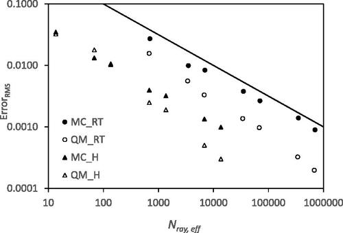
Table 4. View factor system, computational effort to achieve 0.001 average RMS error.

Method	Nray	Nfun	trel	Nray,eff	Speed-up
MC_RT	630,000	–	1	8,000	1
QM_RT	67,000	–	0.97	65,000	9.7
MC_H	–	690,000	0.019	13,000	48
QM_H	–	65,000	0.019	1,300	480

6. Conclusion

In this article a hybrid Monte-Carlo method is applied to two view factor configurations and a view factor system. For the view factor configurations, the numerical behavior of the hybrid Monte-Carlo method is demonstrated to be very different to the standard Monte-Carlo method combined with ray tracing. A key aspect of the hybrid Monte-Carlo method is the number of rays traced is minimized, being restricted to surfaces with a common edge or point. The hybrid Monte-Carlo method demonstrates significant reduction in run-time to achieve the same error compared to a Monte-Carlo method based on ray tracing.

For view factor systems the evaluation of the different variants of the Monte-Carlo method is not as straight forward as for view factor configurations. For MC_RT rays are allocated to emitting surfaces and all view factors for each emitting surface can then be evaluated. For the hybrid Monte-Carlo method function evaluations are allocated to individual view factors. This has two advantages: view factor algebra can be applied to reduce the number of view factors calculated using a Monte-Carlo method and it is possible to allocate a different number of function evaluations to each view factor calculated, taking advantage of the functional form of the integral kernel (10(10) $$F_{E,R}=\frac{1}{A_E}{\int }_{A_E}^{\mathrm{ }}{\int }_{A_R}^{\mathrm{ }}\frac{-\left(x_E-x_R\right).n_E\mathrm{ }\left(x_E-x_R\right).n_R}{\pi {\left(\left(x_E-x_R\right).\mathrm{ }\left(x_E-x_R\right)\right)}^2}d{A}_R\mathrm{ }d{A}_E$$(10) ). A weighting factor for the asymmetric allocation of function evaluations is proposed based on the surface area of the emitting and receiving surface and the distance between the surface centers. Some numerical experimentation and the dependence of the average RMS error on the distribution of function evaluations [X_i,j], suggests the weighting function is not critical to producing a reduction in the average RMS error.

For the view factor system, a composite speed-up of 48 for MC_H and a composite speed-up of 480 for QM_H relative to MC_RT are achieved. The improvement in efficiency using the hybrid Monte-Carlo method is primarily to do with the reduced run-time for a single function evaluation compared to a ray trace. As the number of surfaces increases the divergence in run-time would increase as the number of potential ray intersections scales with the number of surfaces. At some point a domain partitioning algorithm [22–24] is likely to change the efficiency in favor of ray tracing, tending to reduce the speed-up parameter.

Considering possible future work, pairs of view factors and view factor triples taken from the view factor system are used to derive the weighting function (40)(40) $$X_{i,j}=\raisebox{1ex}{$\frac{{\left(A_i{A}_j\right)}^{n_1}}{{\left|z_i-z_j\right|}^{n_2}}$}\!\left/ \!\raisebox{-1ex}{$\Sigma $}\right.$$(40) used to allocate function evaluations to view factors. This is a partially circular argument, and it is important that the universality of the weighting function be explored using other view factor systems. Of all the modifications of the hybrid Monte-Carlo method this one gives a marginal gain for a minor increase in complexity of the algorithm.

A further consideration is the view factor system considered has no internal surfaces. A view factor system with internal surfaces requires some modification of the hybrid Monte-Carlo method, increasing the checking for intersections of lines with the internal surfaces. This will degrade the efficiency of the hybrid Monte-Carlo methods. A view factor system with internal surfaces would also give an integral kernel of (10)(10) $$F_{E,R}=\frac{1}{A_E}{\int }_{A_E}^{\mathrm{ }}{\int }_{A_R}^{\mathrm{ }}\frac{-\left(x_E-x_R\right).n_E\mathrm{ }\left(x_E-x_R\right).n_R}{\pi {\left(\left(x_E-x_R\right).\mathrm{ }\left(x_E-x_R\right)\right)}^2}d{A}_R\mathrm{ }d{A}_E$$(10) with a discontinuity which is likely to degrade the performance of the quasi-Monte-Carlo method as the smoothness assumption of the integral kernel is violated.

Nomenclature
AE, AR	=	Area of emitting surface and receiving surface (m2).
dAE, dAR	=	Differential areas of an emitting and receiving surface (m2).
fE, fR	=	2 Dimensional manifolds representing the emitting and receiving surface.
Fi, j	=	View factor between surface i and j (–).
$\widetilde{F_{i, j}}$	=	Approximate view factor (–).
Fi	=	Function evaluation in the numerical integration methods.
I, In	=	Exact and approximate value of an integral.
MC_H	=	Hybrid Monte-Carlo method.
MC_RT	=	Monte-Carlo method combined with ray tracing.
Nsurf	=	Number of surfaces.
nE, nR	=	Orientation vector for emitting and receiving surfaces.
Nfun	=	Number of function evaluations used to evaluate a view factor.
$N_{\mathit{fun},a2}$	=	Number of function evaluations used to evaluate the view factor $F_{a2-b}$ (–).
$N_{\mathit{ray},a1}$	=	Number of rays traced to evaluate the view factor $F_{a1-b}$ (–).
Ni	=	Number of function evaluations in the numerical integration methods.
NRay E, R	=	Number of rays emitted from surface E intersecting the receiving surface R.
NRay, E	=	Total number of rays emitted from surface E.
Nray	=	Number of rays traced to evaluate a view factor.
Nsample	=	Number of samples used to calculate an average relative error or average RMS error.
QM_H	=	Hybrid quasi-Monte-Carlo method.
QM_RT	=	Quasi-Monte-Carlo method combined with ray tracing.
Rai	=	Pseudo random numbers or quasi-random numbers in the unit interval.
tMC_RT	=	Run-time required to trace a single ray using MC_RT (sec).
tQM_H	=	Run-time required to evaluate the integral kernel using QM_H (sec).
trel, QM_H	=	Relative run-time of QM_H compared to MC_RT (–).
VF	=	Variation of the integral kernel (23)(23) $$V_F=100\frac{F_{\max }-F_{\min }}{0.5\left(F_{\max }+F_{\min }\right)}$$(23) .
VF_CYL	=	View factor configuration, cylindrical shell to a coaxial cylindrical shell.
VF_DISK	=	View factor configuration, disk to a parallel coaxial disk.
xE, xR	=	Point vectors on the emitting and receiving surface.
Xhybrid	=	Parameter used to separate the emitting surface into two sub-surfaces, (m).
Xi,j	=	Proportion of function evaluations allocated to calculate Fi,j.

Greek Letters
φE, θE	=	Angles defining the orientation of a ray (rad).
θE, θR	=	Angles a ray makes with the surface orientation vectors for the emitting and receiving surfaces (rad).

Disclosure statement

No potential conflict of interest was reported by the author(s).

References

- M. F. Modest, Radiative Heat Transfer, 2nd ed. New York: Academic Press, 2003.
- P. S. Cumber, “View factors – When is ray tracing a good idea?” Int. J. Heat Mass Transfer, vol. 189, pp. 122698, June 2022. DOI: 10.1016/j.ijheatmasstransfer.2022.122698.
- P. S. Cumber, “Evaluating view factors using a hybrid Monte-Carlo method,” ASME J. Heat Transfer, vol. 144, no. 12, pp. 122801, Dec 2022. DOI: 10.1115/1.4055516.
- J. R. Howell and K. J. Daun, “The past and future of the Monte Carlo method in thermal radiation transfer,” ASME J. Heat Transfer, vol. 143, no. 10, pp. 100801–1, Oct 2021. DOI: 10.1115/1.4050719.
- M. K. Gupta, K. J. Bumtariya, H. A. Shakla, P. Patel, and Z. Khan, “Methods for evaluation of radiation view factor: a review,” Mater. Today: Proc., vol. 4, no. 2, pp. 1236–1243, 2017. DOI: 10.1016/j.matpr.2017.01.143.
- S. Mazumder and M. Ravishankar, “General procedure for calculation of diffuse view factors between arbitrary planar polygons,” Int. J. Heat Mass Transfer, vol. 55, nos. 23–24, pp. 7330–7335, Nov 2012. DOI: 10.1016/j.ijheatmasstransfer.2012.07.066.
- J. Glyn, Modern Engineering Mathematics. UK: Pearson Education Limited, 1992.
- S. J. Hoff and K. A. Janni, “Monte Carlo technique for determination of thermal radiation shape factors,” Trans. Am. Soc. Agric. Eng., vol. 32, pp. 1023–1028, 1989. DOI: 10.13031/2013.31108.
- A. R. Hajji, M. Mirhosseini, A. Saboonchi, and A. Moosavi, “Different methods for calculating a view factor in radiative applications: strip to in-plane parallel semi-cylinder,” J. Eng. Thermophys., vol. 24, no. 2, pp. 169–180, 2015. DOI: 10.1134/S1810232815020071.
- M. R. Vujičić, N. P. Lavery, and S. G. R. Brown, “View factor calculation using the Monte Carlo method and numerical sensitivity,” Commun. Numer. Meth. Eng., vol. 22, no. 3, pp. 197–203, 2006. DOI: 10.1002/cnm.805.
- M. Mirhosseini and A. Saboonchi, “View factor calculation using the Monte Carlo method for a 3D strip element to circular cylinder,” Int. Commun. Heat Mass Transfer, vol. 38, no. 6, pp. 821–826, July 2011. DOI: 10.1016/j.icheatmasstransfer.2011.03.022.
- J. D. Maltby and P. J. Burns, “Performance, accuracy and convergence in a three-dimensional Monte-Carlo radiation heat transfer simulation,” Numer. Heat Transfer. B, vol. 19, no. 2, pp. 191–209, 1991. DOI: 10.1080/10407799108944963.
- M. R. Vujicic, N. P. Lavery, and S. G. R. Brown, “Numerical sensitivity and view factor calculations using the Monte Carlo method,” Proc. Inst. Mech. Eng., Part C: J. Mech. Eng. Sci., vol. 220, no. 5, pp. 697–702, 2006. DOI: 10.1243/09544062JMES139.
- T. Walker, S.-C. Xue, and G. W. Barton, “Numerical determination of radiative view factors using ray tracing,” ASME J. Heat Transfer, vol. 132, no. 7, 2010. DOI: 10.1115/1.4000974.
- F. He, J. Shi, L. Zhou, W. Li, and X. Li, “Monte Carlo calculation of view factors between some complex surfaces: rectangular plane and parallel cylinder, rectangular plane and torus, especially cold-rolled strip and W-shaped radiant tube in continuous annealing furnace,” Int. J. Therm. Sci., vol. 134, pp. 465–474, Dec 2018. DOI: 10.1016/j.ijthermalsci.2018.05.050.
- M. Mirhosseini, A. Rezania, and L. Rosendahl, “View factor of solar chimneys by Monte Carlo method,” Energ. Proc., vol. 142, pp. 513–518, Dec. 2017. DOI: 10.1016/j.egypro.2017.12.080.
- M. Biolabeling, “An efficient Monte Carlo approach for determining shape factors,” Int. J. Mech. Eng. Ed., vol. 33, pp. 39–44, Jan. 2005. DOI: 10.7227/IJMEE.33.1.3.
- P. L'Ecuyer, “Quasi-Monte Carlo methods in finance,” IEEE, Proc. Winter Simulat. Conf., vol. 2, pp. 573–583, 1645. DOI: 10.1109/WSC.2004.1371512.
- P. S. Cumber and P. Wilkinson, “Signal processing, Sobol sequences and hot sampling: calculation of incident heat flux distributions surrounding diffusion flames,” Int. J. Heat Mass Transfer, vol. 54, nos. 21–22, pp. 4689–4701, Oct 2011. DOI: 10.1016/j.ijheatmasstransfer.2011.06.008.
- I. A. Antonov and V. M. Saleev, “An economic method of computing LP tau-sequences,” USSR Comp. Math. Math. Phys., vol. 19, no. 1, pp. 252–256, 1979. DOI: 10.1016/0041-5553(79)90085-5.
- A. Frank, W. Heidemann, and K. Spindler, “Modeling of the surface-to-surface radiation exchange using a Monte Carlo method,” J. Phys.: Conf. Ser., vol. 745, pp. 032143, 2016. DOI: 10.1088/1742-6596/745/3/032143.
- S. Mazumder, “Methods to accelerate ray tracing in the Monte Carlo method for surface-to-surface radiation transport,” ASME J. Heat Transfer, vol. 128, no. 9, pp. 945–952, Sep. 2006. DOI: 10.1115/1.2241978.
- V. Havran, T. Kopul, J. Bittner, and J. Zara, “Fast robust BSP tree traversal algorithm for ray tracing,” J. Graph. Tools, vol. 2, no. 4, pp. 15–23, 1997. DOI: 10.1080/10867651.1997.10487481.
- S. Mazumder and A. Kirsch, “A fast Monte-Carlo scheme for thermal radiation in semiconductor processing applications,” Numer. Heat Transfer, B, vol. 37, pp. 185–199, 2000. DOI: 10.1080/104077900275486.
- R. P. Taylor, R. Lock, B. K. Hodge, and W. G. Steel, “Uncertainty analysis of diffuse-grey radiation enclosure problems,” J. Thermophys. Heat Transfer., vol. 9, no. 1, pp. 63–69, 1995. DOI: 10.2514/3.629.
- K. J. Daun, D. P. Morton, and J. R. Howell, “Smoothing Monte Carlo exchange factors through constrained maximum likelihood estimation,” ASME J. Heat Transfer, vol. 127, no. 10, pp. 1124–1128, Oct 2005. DOI: 10.1115/1.2035111.
- M. E. Larsen and J. R. Howell, “Least-squares smoothing of direct-exchange areas in zonal analysis,” ASME, J. Heat Transfer, vol. 108, no. 1, pp. 239–242, Feb 1986. DOI: 10.1115/1.3246898.
- C. V. S. Murty and B. S. N. Murty, “Significance of exchange area adjustment in zone modelling,” Int. J. Heat Mass Transfer, vol. 34, no. 2, pp. 499–503, Feb 1991. DOI: 10.1016/0017-9310(91)90268-J.
- M. E. Kounalakis, J. P. Gore, and G. M. Faeth, “Turbulence/radiation interactions in nonpremixed hydrogen/air flames,” SY P. (Int.) Combust., vol. 22, no. 1, pp. 1281–1290, Jan 1989. DOI: 10.1016/S0082-0784(89)80139-0.
- P. S. Cumber and O. Onokpe, “Turbulent radiation interaction in jet flames: sensitivity to the PDF,” Int. J. Heat Mass Transfer, vol. 57, no. 1, pp. 250–264, Jan 2013. DOI: 10.1016/j.ijheatmasstransfer.2012.10.032.
- P. S. Cumber, “Validation study of a turbulence radiation interaction model: weak, intermediate and strong TRI in jet flames,” Int. J. Heat Mass Transfer, vol. 79, pp. 1034–1047, Dec 2014. DOI: 10.1016/j.ijheatmasstransfer.2014.08.073.
- P. S. Cumber, “Efficient modelling of turbulence–radiation interaction in hydrogen jet flames,” Numer. Heat Transfer, B, vol. 63, no. 2, pp. 85–114, 2013. DOI: 10.1080/10407790.2013.740395.
- S. B. Pope, “A Monte Carlo method for the PDF equations of turbulent reactive flow,” Combust. Sci. Technol., vol. 25, nos. 5–6, pp. 159–174, 1981. DOI: 10.1080/00102208108547500.
- P. S. Cumber, “Application of the PDF transport model to non-reacting jets using an adaptive Monte-Carlo method,” Numer. Heat Transfer, Part B, vol. 70, no. 2, pp. 91–110, 2016. DOI: 10.1080/10407790.2016.1177414.
- W. P. Jones and Y. Prasety, “Probability density function modelling of premixed turbulent opposed jet flames,” Symp. (Int.) Comb., vol. 26, no. 1, pp. 275–282, 1996. DOI: 10.1016/S0082-0784(96)80226-8.
- P. Lindstedt and E. M. Vaos, “Transported PDF modelling of high-Reynolds-number premixed turbulent flames,” Combust. Flame, vol. 145, no. 3, pp. 495–511, May 2006. DOI: 10.1016/j.combustflame.2005.12.015.
- R. I. Loehrke, J. S. Dolagham, and P. J. Burns, “Smoothing Monte-Carlo exchange factors,” ASME J. Heat Transfer, vol. 117, no. 2, pp. 524–526, May 1995. DOI: 10.1115/1.2822557.
- J. R. Howell, A Catalog of Radiation Configuration Factors, New York: McGraw-Hill, 1982.
- R. Fletcher, Practical Methods of Optimization, vol. 1. New York: John Wiley, 1980.