Benchmark dose (BMD) modeling: current practice, issues, and challenges

Abstract

Benchmark dose (BMD) modeling is now the state of the science for determining the point of departure for risk assessment. Key advantages include the fact that the modeling takes account of all of the data for a particular effect from a particular experiment, increased consistency, and better accounting for statistical uncertainties. Despite these strong advantages, disagreements remain as to several specific aspects of the modeling, including differences in the recommendations of the US Environmental Protection Agency (US EPA) and the European Food Safety Authority (EFSA). Differences exist in the choice of the benchmark response (BMR) for continuous data, the use of unrestricted models, and the mathematical models used; these can lead to differences in the final BMDL. It is important to take confidence in the model into account in choosing the BMDL, rather than simply choosing the lowest value. The field is moving in the direction of model averaging, which will avoid many of the challenges of choosing a single best model when the underlying biology does not suggest one, but additional research would be useful into methods of incorporating biological considerations into the weights used in the averaging. Additional research is also needed regarding the interplay between the BMR and the UF to ensure appropriate use for studies supporting a lower BMR than default values, such as for epidemiology data. Addressing these issues will aid in harmonizing methods and moving the field of risk assessment forward.

Keywords:

• Benchmark dose
• BMD
• BMDS
• PROAST
• NOAEL
• risk assessment
• modeling issues
• model restriction
• model choice
• model averaging

1. Introduction

The benchmark dose (BMD) approach was introduced more than 30 years ago as a way of refining the estimate of the point of departure (POD, also known as the reference point [RP]) (Crump 1984; Stara and Erdreich 1984; Dourson et al. 1985). Additional publications and workshops followed (Farland and Dourson 1992; Leisenring and Ryan 1992; Hertzberg and Dourson 1993; Allen et al. 1994a, 1994b; Barnes et al. 1995; Kavlock et al. 1995; US EPA 1995; Slob 2002; Brown and Strickland 2003; Slob 2014a, 2014b). The first BMD-based safe dose, specifically for methylmercury, was loaded onto EPA’s Integrated Risk Information System (IRIS) in 1995. Guidance and general descriptions on the use of the BMD followed (Klaassen 1995; US EPA 2000; EFSA 2009; EFSA 2017). With this level of guidance and acceptance from regulatory agencies, BMD modeling is now considered the preferred approach for deriving PODs/RPs for developing “safe dose” estimates such as reference doses (RfDs), acceptable daily intake values (ADIs), or similar values, generically termed “risk values” in this article.

The advantages of the BMD are that it can be any dose level, takes the entire dose–response curve into account, and is based on a consistent response level across studies and study types. In contrast, the disadvantages associated with the use of no-observed-adverse-effect levels (NOAELs) or other direct tested study doses as the POD are well documented (Crump 1984; Dourson et al. 1985; Kimmel and Gaylor 1988; Barnes et al. 1995; US EPA 2012; EFSA 2017). These include:

• The NOAEL is limited to the experimental doses tested;

• NOAELs are based on a single data point of a single effect and, therefore, ignore most of the available dose–response information of this single effect;

• The observed experimental response at the NOAEL may vary between studies, making it harder to compare studies;

• The NOAEL approach does not allow estimation of the probability of response for any dose level;

• Studies conducted with fewer animals per dose group tend to yield higher NOAELs due to decreased statistical sensitivity. This is the opposite of what one might desire in a regulatory context because there is a disincentive for better designed, larger studies.

An additional advantage to BMD modeling is that it allows for a more efficient use of animals, allowing more information and better estimates to be obtained from a given number of animals in an experiment, compared with the NOAEL approach (Gaylor et al. 1985; Slob 2014a, 2014b).

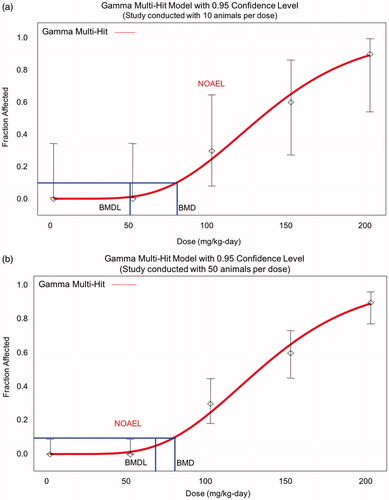
The last bullet may require some additional explanation. A primary advantage of using a BMD vs. a NOAEL is that the former more appropriately accounts for study size (and thus the study’s statistical power), and allows consistent comparison across studies via use of a consistent benchmark response (BMR). For example when using the NOAEL, real differences in response rates among groups may be deemed statistically insignificant if the study has insufficient power, leading to identification of an inappropriately high NOAEL for the study with lower confidence. By contrast, using the BMD approach, confidence limits around the BMD will be tighter for better studies and better models, and the resulting lower bound estimates on the BMD (i.e. BMDLs) will be higher (with smaller studies or poorer models having wider confidence limits and lower BMDLs), all other things being equal (Figure 1). Thus, the BMD approach appropriately reflects the greater degree of precision afforded by a larger study or a better experimental model, resulting in more confidence in the results.

Figure 1. Implication of sample size on NOAEL and BMDL. (a) When there are only 10 animals/group, the response at 100 mg/kg/d in this example is not statistically significant, and so may be considered a NOAEL, but the BMDL is close to 50 mg/kg/d. (b) The greater study sensitivity with 50 animals/group means that the same fraction affected at 100 mg/kg/d is now statistically significant, and so 50 mg/kg/d is considered a NOAEL, but the BMDL is higher than in Figure 1(a). Thus, the BMDL appropriately reflects study sensitivity.

Despite wide acceptance of the BMD approach, there are a number of issues related to its application that can be challenging or confusing, both for novices and sometimes even for experienced risk assessors. There are also several aspects where differences in opinion exist, and/or where guidance continues to evolve. In particular, the European Food Safety Authority (EFSA 2017) and the US Environmental Protection Agency (US EPA 2012) have both developed guidance documents for BMD derivations that differ on several key issues. The purpose of this article is to identify areas where consensus exists and areas where different perspectives exist. Identification of areas of consensus and of disagreement is important in moving toward harmonization, that is transparency, communication, and a shared understanding of approaches, not necessarily standardization (Sonich-Mullin et al. 2001; Rhomberg et al. 2011). Case studies are used to highlight differences in approach and the implication of such differences. In addition, the article identifies and addresses several key areas of confusion among risk assessors. However, this article is not intended as an exhaustive review of the literature or all aspects of the state-of-the-science with regard to BMD modeling. It is also noteworthy that a WHO project to update its guidance on BMD modeling is underway and will address several of the key differences between the US EPA and EFSA guidance at greater depth, particularly from the statistical perspective.

2. Issues

2.1. General description of the method

BMD modeling is conceptually relatively simple. A flexible mathematical model (or group of models) is fit to experimental data, and the dose corresponding to a defined response level is identified. The defined response level is termed the BMR, and the corresponding dose is termed the BMD¹; most risk assessment applications use the lower 95% confidence limit on the BMD (i.e. the BMDL) and EFSA (2017) also recommends that the entire confidence interval (i.e. including the upper bound on the BMD, that is, the BMDU) be described.

In practice, there are several additional potential challenges to BMD modeling. First, unlike the approach using a NOAEL or lowest observed adverse effect level (LOAEL), where the study NOAEL/LOAEL can often be identified by inspection of the study data, it is often necessary to model more than one endpoint in order to identify the critical effect². This is because the endpoint with the lowest NOAEL is not necessarily the endpoint with the lowest BMDL, due to differences in the response in the low dose region, the slope, and potential differences in bounds between dichotomous and continuous endpoints. In practice, a rule of thumb is to model all endpoints with a LOAEL within a factor of 10 of the lowest LOAEL in the database. Evaluation of multiple models for multiple endpoints also can make the modeling process more time consuming than use of the NOAEL/LOAEL approach, although user-friendly software enhancements (BMDS and PROAST) over the past several years have helped to decrease the time needed. Some additional mathematical sophistication is needed to ensure the modeling is done properly and to appropriately interpret the model results, although again the availability of user-friendly software and guidance documents have lowered the barriers to use of BMD modeling. Finally, differences in interpretation can also result with BMD modeling, as discussed in more detail below, although guidance documents (US EPA 2012; EFSA 2017) and ongoing efforts at harmonization aim to decrease such differences, which are probably no larger than similar interpretation differences for the NOAEL approach.

As described in the rest of this critical review, there are also several areas of active discussion or disagreement relating to this deceptively simple series of steps. Differences exist between the US EPA (2012) and EFSA (2017) guidance and associated software in the mathematical models used, the reasons for choosing those models, appropriate constraints on model parameters, and the approach used to choose a final model and associated BMD(L), or whether model averaging should be used instead of choosing a single model.

Before addressing the specific issues related to the modeling and its application, it is useful to provide some additional brief background on the specifics of the modeling. Risk can be expressed as either “additional risk” or “extra risk.” Additional risk expresses the increased probability of response over background. Extra risk takes into account the background response and is essentially the additional risk in the animals that do not develop the endpoint under consideration spontaneously. When the background incidence of a particular effect is small, the BMD results are comparable between these two approaches; when the background is large, there is a larger difference between the additional and extra risk. (1) $$\text{Additional risk is defined as y}\left(\text{d}\right)=\text{ p}\left(\text{d}\right)\hspace{0.17em}–\hspace{0.17em}\text{p}\left(0\right)$$(1) (2) $$\text{Extra risk is defined as y}\left(\text{d}\right)=\left[\frac{\text{p}\left(\text{d}\right)\hspace{0.17em}–\hspace{0.17em}\text{p}\left(0\right)}{\text{1}-\text{p}\left(0\right)}\right]$$(2) where p(d) and p(0) are the risks at dose d or background, respectively. Risk here can be the probability of adverse response in an individual, or the fraction responding in a population. Both the US EPA (2012) and EFSA (2017) recommend the use of extra risk.

Three general types of data can be addressed in the modeling: dichotomous data, continuous data, and nested data. Dichotomous data, also known as quantal data, reflect the count or incidence of some endpoint. Histopathology data are a common type of dichotomous data³. In order to model dichotomous data, one needs the number affected and total sample size at each dose level. Continuous data can be any value (usually a positive value) on the number line. Endpoints associated with continuous data include body weight, serum chemistry, and hematology parameters. In order to model continuous data, one needs the mean and a measure of variability (e.g. the SD) at each dose level, as well as the sample size.

The third type of data is nested data, which are most commonly encountered in developmental toxicity studies. The data are described as nested, because the individual responses (presence or absence of effect in a fetus) are grouped (nested) within the experimental unit, the litter. Models for nested data are currently only in US EPA’s BMDS software, not in PROAST. BMDS has models only for nested dichotomous data, not for nested continuous data. In order to model nested dichotomous data, one needs the incidence of the effect of interest in each litter for each dose. These models reflect the underlying biology, in which effects in the litter are related to the physiology of the dam. Classical statistical analyses of developmental toxicity data should be conducted on a per litter basis rather than a per pup basis, since fetuses from the same dam are not statistically independent. However, the models in BMDS are able to predict fetal risk, while appropriately taking into account the similarity among fetuses from the same dam. It can do this in two ways. First, the software can take into account within-litter similarity due to features of the dam prior to dosing that may be correlated with the outcome of interest (the litter specific covariate); dam weight is a common litter-specific covariate. It can also account for within-litter similarity in response to treatment (intra-litter correlation). This latter covariate reflects the tendency of littermates to respond more similarly to one another relative to the other litters in a dose group, due in part, to the fact that the mother’s internal dose (due to individual toxicokinetics) is a critical determinant of the dose to the pups. Inclusion of the intra-litter correlation helps to ensure that the variance is appropriately estimated, avoiding mis-specification of confidence limits. Thus, the models for nested data capture both the distribution of responses within a litter, as well as the underlying probability of response that varies from litter to litter. Use of these models is more time-consuming than the standard dichotomous models, since incidence data need to be input for each litter individually⁴. Furthermore, since such data are not usually provided in published studies, this modeling usually requires access to the original (often unpublished) study report.

Although BMD modeling is the currently preferred approach for most risk assessments, it may not be possible to apply it to all data sets of interest, because not all data sets are amenable to BMD analysis. Some older studies, particularly acute studies where the expected control response is zero, may report only that specific effects were observed, without any incidence data. Other studies may report central tendency estimates (e.g. mean values), but not a measure of variability, as is necessary to model continuous data. One could reasonably argue that such studies are of inherently low quality and should not be used to derive any sort of risk value. However, in some cases, there may not be other alternatives to deriving a risk value or having some estimate of a risk value to protect public health, and a risk management decision may be made to use poor data in the absence of good data. In other cases, these limited data provide an important part of the weight of evidence, even if they are not used as the basis for a risk value. This could be done qualitatively or semi-quantitatively, or more formally, using such data in a Bayesian approach to help define prior estimation values. In still other cases, the risk assessor may wish to look holistically at several different related measures (e.g. different hematology parameters; or considering data on clinical chemistry, histopathology, and liver weight) to identify a biological threshold and thus an appropriate POD, while BMD modeling forces one to focus separately on the dose-response for each endpoint. In such cases, each endpoint will have a somewhat different BMDL, and it becomes necessary to choose one endpoint of a spectrum of related endpoints as the basis for the POD, while several lines of reasoning from several related endpoints may all point to the same NOAEL.⁵ Another situation might be if there is no dose-response for incidence, due to high background, but there is a clear increase in severity with dose. In some cases, studies with small “n” may be of particular interest because they have been conducted with larger experimental animals (e.g. dogs), for which standard study protocols recommend smaller sample sizes. For such cases, a question arises of whether the greater uncertainty associated with such small samples (and associated wide confidence limits) would be balanced by the greater relevance of experimental animal species, perhaps suggesting a preference for a NOAEL over a BMDL with wide confidence limits. Finally, US EPA (2012) states that BMD modeling is not recommended in cases where the response in all dose groups is high, since extrapolation to the range of the BMR is too uncertain. In such cases, US EPA (2012) recommends obtaining more data or using the NOAEL/LOAEL approach. It is noted, however, that, for many or most of the scenarios identified in this paragraph, analysts with a mathematical focus will often prefer BMD modeling, due to the rigorous and consistent statistical nature of the approach, while more biologically focused assessors may prefer alternative approaches that allow for additional integration of non-quantitative inputs.

The determination of whether BMD modeling or another approach is used may also depend on the problem formulation. For example using NOAELs may be adequate for a screening analysis where a risk management decision needs to be made in less than a day, while BMD modeling may be essential for quantitative evaluations, such as sensitivity analyses or uncertainty characterization, or for a major decision involving exposures of large numbers of people. The problem formulation may also be part of the considerations for addressing several of the other issues addressed in this article.

It is also noted that data sets with small “n” will typically have large confidence limits, potentially resulting in BMDLs much smaller than the associated NOAELs. Often such BMDLs would be preferred, as more appropriately reflecting the uncertainties in the data. However, for certain study types, such as neurotoxicity data, the use of multiple assays measuring closely related endpoints may give the assessor a higher level of certainty about a reasonable starting point (e.g. a BMD) than are reflected in the statistical limits for any single assay or endpoint. Specialized BMD modeling approaches have been developed for such data sets (Zhu et al. 2005).

2.2. Choice of the BMR

Both EFSA (2017) and US EPA (2012) focus on the 10% response range in determining the BMR for dichotomous data, for similar reasons, although the implementation specifics differ. EFSA (2017) notes that “various studies” estimated that the median of the upper bounds of extra risk at the NOAEL was close to 10%, suggesting that the BMDL₁₀ may be an appropriate default (Allen et al. 1994a; Fowles et al. 1999; Sand et al. 2011). BMRs in this range also tend to be in the range of experimental data and thus minimize model dependence.

US EPA (2012) avoids providing default BMRs, but provides the following guidance regarding the choice of BMR for dichotomous endpoints:

• An extra risk of 10% is recommended as a standard reporting level for quantal data, for the purposes of making comparisons across chemicals or endpoints. The 10% response level has customarily been used for comparisons because it is at or near the limit of sensitivity in most cancer bioassays and in noncancer bioassays of comparable size. Note that this level is not a default BMR for developing PODs or for other purposes.

• Biological considerations may warrant the use of a BMR of 5% or lower for some types of effects (e.g., frank effects), or a BMR greater than 10% (e.g., for early precursor effects) as the basis of a POD for a reference value.

• Sometimes, a BMR lower than 10% (based on biological considerations) falls within the observable range. From a statistical standpoint, most reproductive and developmental studies with nested study designs easily support a BMR of 5%. Similarly, a BMR of 1% has typically been used for quantal human data from epidemiology studies. In other cases, if one models below the observable range, one needs to be mindful that the degree of uncertainty in the estimates increases. In such cases, the BMD and BMDL can be compared for excessive divergence. In addition, model uncertainty increases below the range of data.

Consistent with the last bullet, EFSA (2017) also notes that “the default BMR may be modified based on statistical or biological considerations. For example, if the BMR is considerably smaller than the observed response(s) at the lowest dose(s), leading to the need to extrapolate substantially outside the observation range, a larger BMR may be chosen.” Additional information on the US EPA perspective on the choice of BMD is provided in the (US EPA 2005) cancer risk assessment guidelines. That guidance, consistent with the general preference among practitioners, recommends that the BMR be biologically reasonable, and it should be based on the lowest POD adequately supported by the data; BMDLs associated with standard responses of 1, 5, and 10% can be presented.

Thus, the US EPA (2012) and EFSA (2017) guidance are largely consistent regarding the BMR for dichotomous data, although the areas of emphasis differ. In contrast, the two organizations took somewhat contrasting approaches to defining the BMR for continuous data.

Both organizations allow for the BMR for continuous data to be based on toxicological grounds, on a general consensus of the degree of change that is considered biologically significant. This approach is an important part of bringing biological considerations into the evaluation. US EPA (2012) describes this as the ideal approach for continuous data, while EFSA (2017) notes this as a potential modification to the default. As an example of the importance of biological significance, very small changes in hematology parameters sometimes are statistically significant due to low variability in the data, but the magnitude of the change is not sufficient for the change to be considered adverse. A small control SD would mean that not much of a change from control is needed in order to reach a BMR defined as a change of 1 control SD (as addressed below).

Both groups also generally steer away from “dichotomizing” the data into responders and non-responders based on a defined adverse response level and then using quantal models. EFSA does not explicitly address the potential for dichotomizing. US EPA (2012) notes the loss of information when dichotomizing data, although it states that this approach may be used when available continuous models are inadequate for the data. In practice, there have been few if any situations in the past 20 years when EPA assessments have dichotomized continuous endpoints.

The two groups differ, however, in the approach when there is not a clear consensus on the degree of change that is adverse. As a second choice after the ideal situation, the US EPA (2012) notes the potential for application of a hybrid approach (Gaylor and Slikker 1990; Crump 1995; Kodell et al. 1995), which fits continuous models to continuous data, and presuming a distribution of the data, calculates a BMD in terms of the fraction affected. The hybrid models are not explicitly implemented in EPA’s BMDS software, but the third option is a modification of the hybrid approach and the most commonly used approach for assessments in the United States. The US EPA (2012) recommends that a BMR corresponding to a change in the control mean response of one control SD always be presented for comparison purposes and that this BMR could be used in the absence of a biological consensus. The choice of one control SD is based on the work of Crump (1995), who determined that, if exposure results in a shift in a normal distribution of response, and if there is a 1% “background” response in the control group, then changing the mean response by 1.1 standard deviations will result in an additional 10% of the animals reaching the abnormal response level.

EFSA (2017) recommends that the BMR for continuous endpoints be defined as a percent change in the mean response. In the absence of an endpoint-specific determination, EFSA (2017) recommends a default of a 5% change in the mean response. This was based on a re-analysis of data from National Toxicology Program (NTP) studies that found that the BMDL₀₅ was, on average, close to the NOAEL (Bokkers and Slob 2007), as well as similar results from studies of fetal weight data (Kavlock et al. 1995). EFSA (2017) also notes that it may be appropriate to choose a higher BMR for endpoints with larger within-group variability, a situation that it likens to using a BMD defined as a change of 1 SD.

It is interesting how the rationales of the two groups reflect differences in priorities (i.e. what the groups are trying to estimate) and differences in areas of comfort with uncertainty. US EPA (2012) recommends that a defined change in the mean not be used as the basis for the BMR in the absence of a consensus on what is adverse, because “the same percent change for different endpoints (with different degrees of variability) could be associated with very different degrees of response.” Conversely, EFSA (2017) expresses concern that defining the BMR in terms of the control variability means that the BMD varies with study-specific factors (measurement error; dosing error; heterogeneity in experimental conditions), and that the resulting BMD “cannot be translated into an equipotent dose in populations with larger within-group variation, including humans.” Clearly, the definition of the BMR includes judgment and elements of science policy.

For nested data, US EPA (2012) notes that the study designs for most developmental studies readily support a BMR of 5% from a statistical perspective. In addition, Allen and colleagues (Allen et al. 1994a, 1994b; Kavlock et al. 1995) found that statistically derived NOAELs from developmental toxicity studies were comparable on average to BMDLs calculated using a BMR of 5% (and closer to that than BMDLs calculated using a BMR of 10%). EFSA (2017) did not address BMRs for nested data.

The US EPA (2005) recommendation to use the lowest POD adequately supported by the data (and the corresponding US EPA (2012) acceptance of using BMRs lower than 10% based on biological considerations and when the BMR is in the observable range) raises the issue of the implication of using BMRs other than 10%, when supported by the data. Figure 2 shows that the implication of a lower BMR varies with the approach used for low-dose extrapolation. When a no-threshold linear extrapolation is applied (e.g. for carcinogens acting via direct DNA reactivity), a lower BMR provides a better approximation of the expected actual shape of the dose–response curve in the low-dose region, because it is closer to the typical shape of the dose–response curve in this region. In other words, most dose–response curves have shallower slopes at low doses than at higher doses, and so extrapolating from a lower POD would better approximate the expected shape of the curve in the very low-dose region. (Compare the lines from POD1 and POD2.) No additional quantitative adjustment is needed, as the BMR is taken into account when extrapolating to an acceptable risk (e.g. extrapolating from a BMR of 2% to an acceptable risk of 1 in 100 000, or 1 in 1 000 000). This approach has been used to improve the dose–response estimate in animal studies with large numbers of animals [e.g. (Dourson et al. 2008) used a BMR of 2%].

Figure 2. Implications of alternative PODs/BMRs. When a no-threshold linear extrapolation is applied, a lower BMR provides a better approximation of the expected actual shape of the dose–response curve in the low-dose region (reflecting the typically shallower slope at low doses than at higher doses). This means that extrapolating from a lower POD would better approximate the expected shape of the curve in the very low-dose region. (Compare the lines from POD1 and POD2.) In contrast, when the endpoint being modeled has a threshold, so that uncertainty factors would be applied in deriving a safe dose, choosing a lower BMR for a given data set will result in a lower RfD (compare RfD1 and RfD2), suggesting that in this case it may be necessary to adjust the UFs to reflect the lower POD.

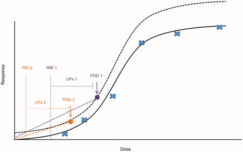
In contrast, when the endpoint being modeled has a threshold, so that uncertainty factors (UFs) would be applied in deriving a safe dose, it may be necessary to adjust the UFs to reflect the lower POD. Consider a chemical with a BMDL derived from a BMR of 10% relative change from controls, the limit of the existing study. When an improved study is selected that allows a BMR of 1% to be used, the corresponding BMDL could be much lower, reflecting the lower BMR and BMD⁶. This raises the question of whether one or more of the UFs should be modified to reflect the lower POD. Application of the same composite UF to a lower POD would automatically result in a lower risk value (compare RfD1 and RfD2, corresponding to POD1 and POD2). Thus, rather than improving the accuracy of the dose–response estimate, using a lower BMR for a threshold effect automatically reduces the final risk value, unless an adjustment is made to the UFs. Crump (1995) also noted this interaction between the BMR and choice of UFs.

The approach to this issue may depend in part on whether the POD comes from an animal study or an epidemiology study. Both US EPA (2012) and EFSA (2017), as well as (US EPA 2002) suggest the potential use of a lower BMR, such as a BMR of 1%, for quantal data from epidemiology studies, since the response is often in this range and use of a 10% response would involve extrapolation upward from the data. However, none of these sources suggest modifying the corresponding UFs, or even address whether the UF should be modified. In the absence of any documentation, the underlying thinking is not clear, but it is worth highlighting some issues that should be considered. One key aspect is recognizing that the overall composite UF is generally lower when extrapolating from epidemiology studies than from animal data, by at least a factor of 10, and often a larger factor. The inherent conservatism in default UFs generally provides some extra margin of safety when extrapolating from animal data, but this additional margin is no longer available with a small uncertainty factor. It would be useful to further investigate the impact of the size of the BMR using actual epidemiology data. To do this, one would calculate the slope at different BMRs, and then determine the number of standard deviations by which the BMD(L) would need to be decreased to result in the response below some targeted percentage of the population. Repeating this for different data sets would provide an estimate of the distribution of slopes, albeit a crude one in light of the expected small number of different chemicals with appropriate data for analysis. Based on this analysis, one could determine the most appropriate UFs for different combinations of slope and BMR for epidemiology data.

It is also worth noting that the BMDL and the UF_H in epidemiology studies both reflect some of the variability in the population, as well as sample size, but in different ways. The BMDL reflects the variability in the sample population based on sampling variability and the resulting uncertainty about the “true” BMD. In contrast, although the UF_H also addresses population variability, it is designed to address how well the population sample reflects the sensitive population. Thus, this factor is often reduced if the study reflects sensitive humans. EPA has used considerations of the degree to which the sensitive population was included in the population sample in its reduction of UF_H from 10- to 3-fold for the RfDs for arsenic, molybdenum, and selenium (Dourson et al. 2001). For all three of these RfDs, large samples of the general population were used to determine the POD that was the basis for the RfD. However, UF_H is not automatically decreased solely because the sample is large, but because it was also heterogeneous. UF_H would not be reduced if a large epidemiology study were conducted in a homogeneous population (e.g. male workers).

Because both the BMDL and the UF_H may reflect different aspects related to the population size, it is worth considering the potential for some interplay between the two parameters. For example if the sample size is small, a full UF_H would generally be used, but the confidence limits would also be expected to be wider, reflecting the small sample size. The use of the wider confidence limits for a smaller study in the general population, together with a full UF_H might be considered to be doubly penalizing the study for the smaller size. Conversely, a large sample size would result in relatively tight confidence limits and a higher BMDL. If a reduced UF_H is used in this case, based on a large sample size that covers the sensitive population, one might consider whether this is giving the study “double credit” for the larger sample size. Thus, it may make sense to have one standard UF_H for epidemiology studies with the same BMR, with the idea that the sample size is accounted for in the lower limit. It would be useful to conduct further research on this issue, using model data sets extracted from real epidemiology data, in order to better characterize the interplay among sample size, BMD, and BMDL, as well as the implication of the choice of BMR and uncertainty factors.

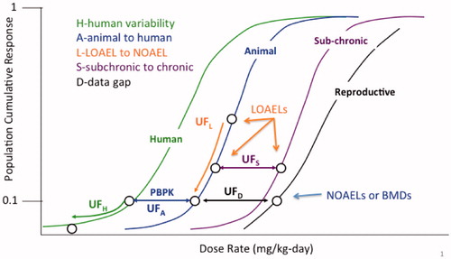
Different considerations apply in addressing whether specific adjustments to the UFs are needed when extrapolating from lower BMDLs in animal studies. But first, some brief background on UFs is needed. Figure 3 shows the use of these factors conceptually on a hypothetical dose–response curve for a threshold toxicant, using the scheme developed by the US EPA (Barnes and Dourson 1988; US EPA 2002). Other organizations’ schemes are similar and also can be used in this comparison. In brief, the areas of uncertainty considered are the following:

• UF_H – human variability, including protection of sensitive populations.

• UF_A – interspecies differences between the experimental animals and humans.

• UF_L – extrapolation from a LOAEL to a NOAEL.

• UF_S – extrapolation from a subchronic study to a chronic/lifetime exposure.

• UF_D – incomplete database, accounting for missing studies, or other database deficiencies.

Figure 3. Typical uncertainty factors used in safe dose assessment. This figure distinguishes among the uncertainty factors that extrapolate between (hypothetical) dose-response curves (i.e. UF_A, UF_S, and UF_D), and those that move down the same dose-response curve (UF_H and UF_L).

Some approaches (IPCS 1994; Meek et al. 1994) combine one or more of the latter three areas of uncertainty into one factor.

Figure 3 shows that only two UFs address reductions in risk: UF_H and UF_L. UF_H lowers the BMD or NOAEL for an average group of humans to a BMD or NOAEL for a sensitive group of humans, thereby lowering the overall risk to the population. UF_L lowers the value of the LOAEL into the expected range of the BMD or NOAEL, thereby lowering the overall risk to the experimental group. The other three factors, UF_A, UF_S, and UF_D, are extrapolations from one hypothetical dose–response curve to another without any corresponding change in the projected (or estimated) risk.

Categorizing the UFs into those that reduce risk and those that move from one hypothetical dose–response curve to another helps in identifying the UFs that would be relevant to a change in the BMR. Because using a BMR different from 10% affects the underlying risk, one should focus on potential modifications to the uncertainty factors UF_H and UF_L if one were to extrapolate from a lower BMR in an animal study. However, as noted, BMDLs are chosen to be equivalent, on average, to a NOAEL, and thus UF_L is generally 1 when BMD modeling is conducted. This raises the question of how to adjust for differences in the BMR while ensuring that sensitive human populations are protected.

This line of thinking suggests that the magnitude of the composite UF (and associated degree of conservatism) be considered in identifying the BMR, to ensure appropriate estimation of the risk value. Thus, for example if extrapolating from an animal study using a chemical-specific adjustment factor (CSAF) (IPCS 2005) or data-derived extrapolation factor (DDEF) (US EPA 2014), it is useful to consider the magnitude of the combined factor and the resulting projected risk. If, for example the total factor is 10 or less and the severity of the critical effect is more than mild, it may be appropriated to consider a lower BMR.

Another issue that relates to the choice of the BMR reflects the interplay between that choice and using the BMD vs. the BMDL as the POD. As noted, the US EPA and several other organizations use the BMDL. That is, the lower bound on the dose is used, as part of a desire to reflect the uncertainty inherent in the data, and the 10% response is commonly used (for quantal data), in order to match, on average, historic NOAELs. But this is not the only combination that can match historic NOAELs on average. Health Canada’s Existing Substances Division has used the BMD instead of the BMDL, since the BMD is more stable statistically, particularly for small sample sizes. In order to be generally consistent with historic NOAELs, Health Canada has used the BMD₀₅, and in many cases, the BMD₀₅ is expected to be in the range of a BMDL₁₀ (personal observations of M. Dourson and L. Haber). However, use of the BMD₀₅ eliminates one of the advantages of the BMD approach, namely appropriately reflecting uncertainty in the point of departure, as discussed above.

2.3. Comparisons of NOAELs to BMDLs

As noted, part of the rationale for the choice of BMRs was based on a goal of having BMDLs agree, on average, with NOAELs. This does not mean, however, that the BMDL for every endpoint will be comparable to the corresponding NOAEL. It is not surprising that some BMDLs will be lower and some will be higher; that is part of the definition of “agree on average.”

Despite these basic definitional considerations, confusion sometimes arises regarding the appropriate approach and interpretation when there are apparent disparities between NOAELs and BMDLs. Sometimes, the BMDL is closer to the LOAEL than the NOAEL, or even higher than the LOAEL. In other cases, the BMDL may be substantially lower than the NOAEL. In considering how to evaluate these cases, it is important to keep in mind that the ultimate goal is to estimate a human dose that is as close as possible to, but still below, the biological threshold for adversity. To achieve this goal, the modeled POD should be near the data (non-control points) but as low as can be reliably and plausibly extrapolated along the fitted dose–response curve. However, it should be recognized that the experimental animal response at the NOAEL is not necessarily zero. In fact, statistical analyses have shown that the response at the NOAEL can be as high as 30% for the standard 10 animals/group in a subchronic study (e.g. US EPA 2012). This potentially higher response is reduced at low levels of human exposure because of the conservatism inherent to the application of uncertainty factors, which are multiplied together. That is, the default uncertainty factors are each based on a high percentile of the relevant distribution (e.g. the difference between human and animal sensitivity) and it is unlikely that the same chemical will fall at the high end of the distribution for all relevant uncertainty factors. Therefore, the use of the default factors (including the default factor of 100) is considered to be protective (Dourson and Stara 1983).

Thus, it is important to consider the data in detail and evaluate the reason for apparent contradictions between the BMD and NOAEL approach, rather than automatically choosing one approach or another. In particular, one should consider how the power of the study and the tightness of the data are reflected in the BMD, BMDL, NOAEL, and LOAEL. For example if the sample size is 10/group, then a 10% change in incidence is a difference in incidence of only 1 animal or subject. This magnitude of change would not be statistically significant, but it would be the basis of a BMD. The BMDL would be even lower, and a high background in the control group would lead to an even smaller BMDL when “extra risk” is used. (High background can be thought of as a smaller “n” of animals that are left able to respond to exposure.) While this may appropriately reflect the uncertainty in the data, a risk assessor may have concerns about allowing such a small change, which could be due to random variation, to drive a very low BMDL. The risk assessor needs to consider the overall dose-response, as well as the nature of the endpoint and historical control data (as an indication of the variability in that high background) in considering whether it is appropriate to use such a low BMDL. Conversely, studies with small “n” may raise the question of whether an adverse change is really occurring, but the dose group size or overall study size is not sufficiently large to allow its detection. Due to the potential impact of small changes in the incidence, some have expressed reluctance to use the BMD approach for datasets with small “n.” In addition, methods to address this issue have been explored specifically for neurotoxicology testing, when a large number of related assays are conducted with the same small group of animals (Zhu et al. 2005), and in general (Leisenring and Ryan 1992; Brown and Strickland 2003).

2.4. Model formulas used for modeling

The next step after identification of the BMR is to identify the mathematical models that will be used for the modeling. This is another area where the US EPA and EFSA guidance differ⁷. Both groups note that the ideal approach is to use a biologically based dose–response (BBDR) model that describes the chemical’s toxicokinetics and toxicodynamics. Both groups also note that it is rare to have such a model and that in the absence of a BBDR, the modeling is largely a mathematical curve-fitting exercise.

EPA and EFSA appear to differ in philosophy on the approach to use to identify candidate models in the absence of a BBDR model. US EPA (2012) states that no recommended model hierarchy was available at the time. Instead, coupled with the BMDS software (U.S. Environmental Protection Agency, Washington, DC), the EPA approach is to use a variety of flexible models. BMDS includes nine dichotomous models, eight “alternative” dichotomous models, and five continuous models (counting the variations on the exponential model as one model).

EFSA (2017) also recommends a variety of flexible models, but within a narrower range. For the continuous models, EFSA (2017) recommends only the 3- and 4-parameter versions of the exponential and Hill models. EFSA notes that the recommended models have the following characteristics:

• They always predict positive values, e.g. organ weight cannot be ≤0.

• They are monotonic (i.e. either increasing or decreasing).

• They are suitable for data that level off to a maximum response.

• They have been shown to describe dose–response data sets for a wide variety of endpoints adequately, as established in a review of historical data (Slob and Setzer 2014).

• They allow for incorporating covariates in a toxicologically meaningful way.

• They contain up to four parameters, which have the same interpretation in both models. families, in particular: a is the response at dose 0, b is a parameter reflecting the potency of the chemical (or the sensitivity of the population), c is the maximum fold change in response compared to background response, and d is a parameter reflecting the steepness of the curve (on log-dose scale).

EFSA (2017) also notes that it no longer recommends the models in these families with fewer parameters, because “BMD confidence intervals tend to have low coverage when parameter d is in reality unequal to one.”

Before continuing to describe the EFSA approach, we wish to add some comments on the EFSA concerns about adequate coverage of confidence intervals. The exponential Hill models with fewer parameters set the power (d) parameters equal to one. So, it would not be surprising if those models had poorer coverage when, in fact, d was greater than 1. But that is somewhat circular: one does not know a priori what the shape of the dose-response is, and dropping those models would not be appropriate when the underlying dose–response shape does have d = 1, except insofar as the 4-parameter models have the d = 1 models as special cases. Although these are special cases, if a restriction is imposed on the power parameter (such that it is greater than or equal to 1, as is often done to assure finite slope near background), then that special case is on the boundary of the allowed parameter space and is worth including on its own.

EFSA (2017) notes that the power and polynomial models of BMDS are not recommended because they are additive with respect to the background response, which could result in fitted curves predicting negative values. While this may be a theoretical concern, it does not seem to be an issue in practice; the authors have never encountered this issue in modeling data sets over many years. Similarly, while it is possible to obtain non-monotonic curves with the polynomial model, these results are avoided by constraining (restricting) the polynomial coefficients so that they are either non-positive or non-negative. The remaining characteristics apply to some, but not all, of the BMDS models, though all apply for at least some of the models. Thus EFSA appears to place more emphasis on all of the suggested models having certain parallel characteristics, rather than ensuring the characteristics are met by having a variety of options.

For dichotomous models, EFSA lists eight recommended models. This list is again largely a subset of the BMDS models, with two deviations. First, EFSA also includes latent variable models based on an underlying continuous response, which is dichotomized based on a (latent) cutoff value that is estimated from the data. In addition, EFSA recommends only the two-stage version of the linearized multistage (LMS) model, while BMDS allows for higher stages. EFSA explains the elimination of the three-stage model as being because it rarely provides a better fit to the data. EFSA also notes that the logit and probit models have only two parameters, and a minimum of three appears to be needed. EFSA states that “it is general experience that these two models provide poor fits to real data sets that include more than the usual number of doses (three plus controls).”

With regard to the differences in choices of models for both dichotomous and continuous endpoints, there appears to be little harm (and some potential benefit) in including the models as options when the BMDL is chosen based on the best-fitting model(s). It is also worth noting that in such cases, the best fitting model has often in our experience been chosen from among the models that EFSA would eliminate. However, when model averaging approaches are applied (see below), it may become more important to limit the suite of models being tested. Model averaging is additionally discussed in Section 2.7.

2.5. Restriction/constraining parameters

One of the significant areas of disagreement between the current US EPA (2012) and the EFSA (2017) guidance relates to restricting (also known as constraining) parameters. The EPA’s guidance is that one should first run the “restricted” models, to avoid biologically problematic dose–response curves, and to run the unrestricted models only if an acceptable fit is not obtained with any of the restricted models. While there is more general agreement that parameters should be restricted to avoid non-monotonic curves, the issue of constraining models that are steeply supralinear is more controversial. US EPA (2012) states:

In general, the modeler should consider constraining power parameters to be 1 or greater (this is the default in the BMDS software…). However, if the observed data do appear supralinear, unconstrained models or models that contain an asymptote term (e.g., a Hill model) warrant investigation to see whether they can support reasonable BMD and BMDL values. If they cannot, other model forms should be considered for a POD; at times, modeling will not yield useful results and the NOAEL/LOAEL approach might be considered, although the data gaps and inherent limitations of that approach should be acknowledged.

The EPA guidance presents a fairly nuanced discussion of this issue, noting that it is not unusual for data in the observed range to be supralinear, such as in the case of a Michaelis–Menten relationship, and so excluding power parameters less than 1 may result in worse fit to the data. In addition, since BMD modeling does not involve extrapolation to very low doses, “the high slopes seen for some unconstrained models near the origin is not in itself a fundamental problem.” However, EPA notes that the calculated BMDs and BMDLs can be very low.

EFSA (2017) removes the recommendation for first running the restricted models, based largely on the work of Slob and Setzer (2014), biomathematicians who have played a key role in the development of BMD methodology for EFSA and US EPA, respectively. Slob and Setzer (2014) state that the concern about infinite slope at zero dose is not a plausible one, since the curve has zero slope at zero dose when the x-axis is log-dose instead of linear dose. Therefore, they argue, there is no biological reason to reject the unrestricted models.

The common argument against the unrestricted models is that the low-dose slope is steep because data are missing in the region of interest. According to this argument, the curve would exhibit a more traditional dose–response shape if the lower-dose data were available, and thus such data sets with an initial steep slope have higher uncertainty. Slob and Setzer (2014) come to a similar conclusion, via somewhat different reasoning. They note for some datasets (where the unrestricted model has very steep low-dose slope), the BMDL is very small, reflecting that insufficient dose–response data are available to provide an estimate of the BMD with reasonable precision. They suggest, however, that, instead of constraining the parameters, that using historical data from comparable studies for comparable endpoints together with the study of interest can result in a usable POD. Interestingly, Slob and Setzer (2014) also note that for the data sets that they evaluated, dose–response curves with infinite slope at zero dose occur for about 50% of the chemicals evaluated. The high prevalence of such cases underlines the importance of the development of consistent guidance on this issue.

This issue of constraining the power parameter is discussed in much greater detail in the WHO manuscript under development mentioned above. There appears to be general agreement that the steep slope reflects uncertainty in the dose-response, due to insufficient data in the low-response region. However, additional discussion is needed regarding the proper approach to deal with this important paucity of data. While an ideal situation might be to repeat the experiment to obtain low-response data, repeating studies is generally avoided due to cost concerns, animal welfare concerns, and sometimes because of the urgency for a decision.

2.6. Model choice

2.6.1. US EPA guidance

US EPA (2012) recommends the following approach for choosing the model to use for calculating a POD. Because in our experience the choice of model is often one of the most controversial aspects of BMD modeling, the US EPA guidance is quoted verbatim (except for removing references to other sections of the US EPA guidance), followed by discussion, to allow each reader to interpret the words of the guidance.

1. Assess goodness-of-fit, using a value of α = 0.1 to determine a critical value (or α = 0.05 or α = 0.01 if there is reason to use a specific model(s) rather than fitting a suite of models).

2. Further reject models that apparently do not adequately describe the relevant low-dose portion of the dose–response relationship, examining residuals and graphs of models, and data.

3. As the remaining models have met the recommended default statistical criteria for adequacy and visually fit the data, any of them theoretically could be used for determining the BMDL. The remaining criteria for selecting the BMDL are necessarily somewhat arbitrary and are suggested as defaults.

4. If the BMDL estimates from the remaining models are sufficiently close (given the needs of the assessment), reflecting no particular influence of the individual models, then the model with the lowest Akaike information criterion (AIC) may be used to calculate the BMDL for the POD. This criterion is intended to help arrive at a single BMDL value in an objective and reproducible manner. If two or more models share the lowest AIC, the simple average or geometric mean of the BMDLs with the lowest AIC may be used. Note that this is not the same as “model averaging”, which involves weighing a fuller set of adequately fitting models. In addition, such an average has drawbacks, including the fact that it is not a 95% lower bound (on the average BMD); it is just the average of the particular BMDLs under consideration (i.e. the average loses the statistical properties of the individual estimates).

5. If the BMDL estimates from the remaining models are not sufficiently close, some model dependence of the estimate can be assumed. Expert statistical judgment may help at this point to judge whether model uncertainty is too great to rely on some or all of the results. If the range of results is judged to be reasonable, there is no clear remaining biological or statistical basis on which to choose among them, and the lowest BMDL may be selected as a reasonable conservative estimate. Additional analysis and discussion might include consideration of additional models, the examination of the parameter values for the models used, or an evaluation of the BMDs to determine if the same pattern exists as for the BMDLs. Discussion of the decision procedure should always be provided.

6. In some cases, modeling attempts may not yield useful results. When this occurs and the most biologically relevant effect is from a study considered adequate but not amenable to modeling, the NOAEL (or LOAEL) could be used as the POD. The modeling issues that arose should be discussed in the assessment, along with the impacts of any related data limitations on the results from the alternate NOAEL/LOAEL approach.

The US EPA (2012) guidance also notes that model averaging is possible, but at the time the guidance was written, additional research and guidance were recommended. As discussed in the following section, model averaging appears to be on the verge of being the state of the science, and not solely a tool for mathematical experts. Model averaging is described by EFSA (2017) as the method of choice. Model averaging capabilities are part of PROAST, and US EPA is actively working on incorporating model averaging capabilities into its BMDS software.

The AIC noted in item (4) above is a measure of overall fit that takes into account the number of model parameters, and is calculated as −2LL + 2p, where LL is the log-likelihood at the maximum likelihood estimates (MLEs) for p estimated parameters. The AIC, rather than the goodness of fit p values, is used to compare model outputs from a data set, to account for the general improvement of fit as additional parameters are added within a family of models. The +2p factor in the AIC equation addresses the question of whether the improvement in fit justifies estimating additional parameters. That is, among models with similar fit, the AIC prefers less complex models. Smaller AICs (to the left on the number line) are better when comparing two models. Note that only the difference in AIC is meaningful, not the actual value. Because the AIC includes an adjustment of 2 times the number of parameters, a difference of 2 in the AIC (a unitless measure) is often considered meaningful, since a difference of that magnitude means that adding the parameters improved the fit more than the penalty for adding the parameters.

A few aspects of US EPA’s guidance are worthy of particular note. First, EPA describes the process of model selection as a two-step process. The first step is identifying which models are acceptable, based on the goodness of fit p values, visual fit, and scaled residuals (a measure of local fit). The second step is the choice of the model (or models, if the BMDLs are averaged) from among those with acceptable fit. The guidance document appears to avoid being prescriptive with regard to the choice of the model, stating that the “the model with the lowest AIC may be used” (emphasis added). Similarly, in the fifth point above, no definition is provided for “sufficiently close” BMDL estimates. This was a conscious decision by EPA to not define sufficiently close; a factor of 3 was specified in the draft guidance. EPA’s training materials state that a factor of no more than 3 can be used, but one can use a smaller factor (Jeff Gift and Allen Davis, personal communication, November 18, 2016).

Despite the generally non-prescriptive nature of this portion of the EPA guidance, in practice, EPA assessments have often been based on the model with the lowest AIC, to the point that many consider it mandatory to choose the model with the lowest AIC, regardless of other fit considerations. Although this approach does result in ease of use, consistency and avoids concerns about the potential for “cherry picking,” it may not always be scientifically justified, such as in cases of poor fit in the low-dose region or when biological understanding would suggest one or more models over the one with the lowest AIC. Also, as noted, small differences in AIC are not considered statistically meaningful. While it appears that modelers consider a value of 2 or more to be a meaningful difference in the AIC for the reason noted above, it is not clear how small the difference can be in AIC values and still be meaningful for model selection purposes. This suggests that, rather than relying solely on the AIC, it is useful to consider all fit criteria more holistically.

In addition to the previously described criteria (i.e. scaled residuals, visual fit, AIC, etc.), the EPA guidance notes the importance of accurately estimating the variances for continuous data sets. The variance parameter is estimated simultaneously with the dose–response model parameters, and so the accuracy of the estimation of the variance affects the model fit parameters. Inaccuracies in the estimate of the variance estimate may bias estimates of the model parameters. In addition, when the BMR is defined in terms of a one standard deviation change in the control mean, accurate estimation of the control variance is essential for an accurate estimation of the BMD(L). Unfortunately, BMDS currently includes only two options for estimating the variance. The variance can be assumed to be constant with dose, or it can be modeled as increasing with dose, proportional to the mean raised to a power. If neither of these two approaches can adequately describe the variance, then a common approach, albeit suboptimal, is to revert to the NOAEL/LOAEL approach. However, mathematically sophisticated analysts can use spreadsheets to fit models with independent variances, that is, separate variance terms for each dose group, that are independent of one another and of the underlying dose–response pattern. In fact, such an approach reflects the least restrictive set of assumptions about the underlying data-generating process. While it requires estimation of additional parameters (dose-specific variance estimates), this is a viable option much preferred over a NOAEL/LOAEL derivation when the interest is primarily on the dose–response pattern rather than the variability around that pattern. In other words, the independent variance approach does not allow one to extrapolate the variance estimates to other dose or response levels. It is possible that the independent variance approach may be incorporated into a future release of BMDS.

The BMD:BMDL ratio is not explicitly addressed in the EPA guidance, although some of the authors of this article see this as part of the guidance (see below). In practice, the BMD:BMDL ratio is part of the output of the Wizard program that is part of BMDS, and large ratios indicate greater uncertainty in estimating the most likely actual BMD value. The use of the BMD:BMDL ratio as one measure of influence of model on BMDL is reasonable to some analysts but not others, and discussed in greater depth in Section 2.8.

The same general approach as for quantal data is used for nested data sets for quantal endpoints, although there are some additional complications. For example the reported scaled residuals are litter-specific, rather than dose-specific. In addition, visual fit generally carries less weight, again reflecting the variability across litters.

2.6.2. EFSA guidance

The EFSA (2017) approach is shown in Figure 4. There is less ambiguity for interpretation in the EFSA guidance than the US EPA approach, and so the EFSA approach is paraphrased in portions here. However, two additional definitions are needed prior to discussing the EFSA approach. As defined by EFSA:

Figure 4. EFSA flowchart for BMD modeling.

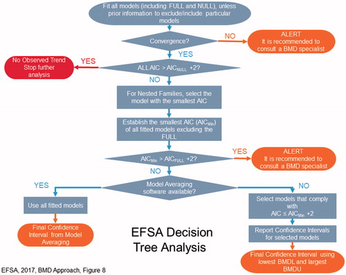
The full model describes the dose–response relationship simply by the observed (mean) responses at the tested doses, without assuming any specific dose–response. It does, however, include the (same) distributional part of the model and thus it may be used for evaluating the goodness of fit of any dose–response model.

The null model expresses the situation that there is no dose-related trend, i.e. it is a horizontal line, and may be used for statistically evaluating the presence of a dose-related trend.

After fitting all of the models (including the full and null models), unless there is prior information to exclude or include particular models, the first step is to evaluate model convergence. If the model did not converge to a single maximum likelihood, it is possible that there may be more than one set of parameter estimates that would result in similar log-likelihood values. The EFSA guidance states that, “convergence may not be critical in providing a reliable BMD confidence interval, and therefore a message of non-convergence does not necessarily imply that the model should be rejected.” Instead, a BMD specialist (not further defined) should be consulted. The lack of convergence could be because the data are not informative or the model may be over-parameterized.

EFSA’s next step is to compare the AIC of the null model with that of the fitted models (i.e. various mathematical expressions used to fit the data), to evaluate for evidence of a dose-related trend. EFSA (2017) states that a model shows statistical evidence of a dose-related trend, if its AIC is less than AIC_null − 2. If the AICs of all of the fitted models are greater than AIC_null – 2, then there is no evidence of trend and no further analysis is conducted.

For nested families, EFSA then chooses the model with the lowest AIC, so that only one model from each family is carried into the next step.

To evaluate adequacy of fit, the AIC is then compared with the AIC of the full model. EFSA (2017) states that “the AIC of a fitted model should be no more than two units larger than the full model’s AIC. If the model with the minimal AIC is more than two units larger than that of the full model (AIC_min > AIC_full + 2), this could be due to the use of an inappropriate dose–response model (e.g. it contains an insufficient number of parameters), or to misspecification of the distributional part of the model (e.g. litter effects are ignored), or to non-random errors in the data.” If AIC_min > AIC_full + 2, it is recommended to consult a BMD specialist.

This approach narrows the models down to those that EFSA considers statistically acceptable. Note that one potential limitation it that the EFSA guidance does not address visual fit or scaled residuals, despite the broad acceptance of these as biologically relevant parameters. Under the EFSA approach, these biologically important parameters of fit are not considered in either the weighting of models for the preferred approach of model averaging or are they considered in the choice of individual models.

At this point, EFSA’s preferred approach is to use model averaging. If the appropriate software is available, all models (excluding the full and null models) are averaged, weighted by the AIC. If model averaging software is not available, then the models are sorted to identify those with “relatively good fit” and “relatively poor fit.” Models with “relatively good fit” are defined as the model with the lowest AIC, and all models with an AIC no more than two units larger than that. EFSA then recommends that one approach is to choose the lowest BMDL of these models. However, EFSA focuses more on the complete confidence interval, reporting the final confidence interval using the lowest BMDL and the highest BMDU. EFSA provides somewhat ambiguous guidance with regard to the choice of the BMDL. Instead of choosing the lowest BMDL, the guidance states:

…this procedure may not be optimal in all cases, and the risk assessor might decide to use a more holistic approach, where all relevant aspects are taken into account, such as the BMD confidence intervals (rather than just the BMDLs), the biological meaning of the relevant endpoints, and the consequences for the HBGV (health-based guidance value) or the MOE (margin of exposure). This process will differ from case to case and it is the risk assessor’s responsibility to make a substantiated decision on what BMDL will be used as the RP (reference point, the term used by EFSA for the POD). One example is a situation where the BMD confidence interval with the lowest BMDL is orders of magnitude wide. This means that the true BMD might be much higher than the BMDL, which raises the question if that BMDL would be an appropriate RP.

The EFSA guidance further states in the context of wide confidence limits:

In some cases, the selected RP may not be the lowest BMDL, for example, when this lowest BMDL concerns an effect that is also reflected by other endpoints (e.g. the combination of liver necrosis and serum enzymes) that resulted in much smaller confidence intervals but with higher BMDLs. In that case, it might be argued that the true BMDs for those analogous endpoints would probably be similar, but one of them resulted in a much wider confidence interval (e.g. due to large measurement errors).

This final approach appears to at least partially address the issue noted in Section 2.1 that BMD modeling has typically been conducted endpoint by endpoint, not allowing the integration across related endpoints that is common in the use of the NOAEL approach to identify a POD. It will be of interest to see examples of cases where several related endpoints are modeled and a BMDL based on an endpoint with tighter confidence limits is used as the POD. See also the discussion of BMD:BMDL ratios in Section 2.8.

2.6.3. A holistic approach

Many of the authors of this article have advocated a holistic approach to model selection. This approach follows the US EPA guidelines, but does not automatically choose the model with the lowest AIC. Instead, it considers multiple measures of fit, including p values, scaled residuals, the visual fit and evaluation of model influence. Like the EFSA approach, models that have AICs that differ by more than 2 from the lowest AIC of the acceptable models are excluded. For data sets where the BMD:BMDL ratios resulting from different models differ greatly, further examination is useful to evaluate those model(s) with large ratios, to determine what aspects resulted in the larger ratios. This examination can help in assessing underlying elements of the data or models that can inform the best choice of model. Biological considerations can be taken into account, preferring models that are concave upward over models that are concave downward, unless there is a biological reason to expect the latter curve shape. Some models may exhibit a perfect visual fit, but have a shape of the dose–response curve that does not appear to be biologically reasonable. Some models have excellent residuals but have larger BMD:BMDL ratios. Some models have larger AICs, but smaller ratios or residuals. All of these considerations are taken into account in identifying the best model(s). Where there is no clearly best model, BMDLs are often averaged for models with similar fit. Alternatively, the lowest BMD and BMDL can be selected as a conservative choice. In all of these situations, however, it is important to be transparent about the rationale for the choice, and to recognize that much of the rationale is based on scientific judgment and science policy, rather than clear scientific distinctions.

This holistic approach has the advantage of including biological judgment, considering fit more broadly (particularly in the low-dose region), and focusing on statistically meaningful differences in AIC, rather than choosing a model based on small differences in AIC. It also allows the assessor to focus on biologically meaningful differences across models, rather than making decisions solely based on statistical considerations. This holistic approach of focusing on biologically meaningful differences is consistent with both US EPA and EFSA guidance, which allows for a role of scientific judgment by the risk assessor within the confines of their decision steps. However, it is acknowledged that consistency using this approach can be challenging, and it is not even guaranteed that a single assessor would always obtain the same conclusion. This can make the holistic approach more challenging in regulatory applications, where consistency and verifiability are critical. Development of quantitative metrics that capture some of the additional considerations included in the holistic approach, including the visual fit, would help to make the holistic approach more systematic. This may be facilitated by the development of modeling averaging methods that reflect local fit (residuals) and visual fit. Specifically, it would be useful to have a way to quantitatively capture whether the curvature of the fitted curve is consistent with biology and the data.

2.6.4. Summary regarding model selection

We have described three different approaches to choose the best model; additional approaches for choosing the best model are possible, particular variations on the holistic approach. It is recognized that some of the issues of model choice will be eliminated by the use of model averaging, which is gaining acceptance. However, as discussed in the next section, model averaging does not completely eliminate the issues discussed above. Instead, issues of whether and how much to consider biological issues are reframed in terms of what method to use to weight the different models.

Finally, it is important to note that some of the differences in approaches to model choice reflect important underlying differences in perspective regarding the goal of the modeling. US EPA (2012) talks about identifying the model that best fits the data, although the thinking at US EPA has now moved toward model averaging. EFSA (2017) states that “the BMD approach does not aim to find the single statistically best estimate of the BMD but rather all plausible values that are compatible with the data. Therefore, the goal is not to find the single best fitting model, but rather to take into account the results from all models applied.” As discussed in Section 2.8, the “best” model identified using statistical metrics sometimes does not lead to the best estimate of the BMD, based on consideration of both biology and statistics. Therefore, although historic practice (and current best practice) is to choose a single model or average BMDLs, there is a utility in considering multiple models, but it is necessary to ensure that these multiple models capture biologically reasonable BMDs. However, the EFSA approach of describing all plausible values that are compatible with the data risks losing important information. Among the plausible values for the BMD (and associated models), some values and models are more plausible than others. Therefore, perhaps a more nuanced goal would be to identify the more plausible values (taking into account biological judgment), and then identify either a “best” estimate (if it is defined as the most plausible), or identify the range of most plausible values.

2.7. Model averaging

There has been a growing trend in chemical risk assessment to better characterize uncertainty and to have the final assessments appropriately reflect the underlying uncertainty (NRC 2008, 2011, 2014).There has also been a growing recognition that picking the “best” model and using the associated BMDL may not fully reflect the true model uncertainty (Wheeler and Bailer 2007; Piegorsch et al. 2013; Ringblom et al. 2014). Model averaging addresses those concerns by including the results of several models (appropriately averaged) when estimating the BMD and characterizing the uncertainty about that estimate (i.e. through calculation of a BMDL). Note that “model averaging” here does not mean calculating the average BMD or BMDL from several different models. Rather, it refers to a (potentially computationally intensive) approach for calculating a weighted average of model-predicted responses as a function of dose. That is, one can think of a dose–response relationship that, at each dose, computes a weighted average of predictions of the individual models, in essence based on a mathematical function that includes each of the individual model functions. The model average BMD is then based on the dose that gives the defined risk (BMR) after appropriate optimization. The associated uncertainties are then used to calculate the corresponding BMDLs. This can be done using either frequentist approaches (Wheeler and Bailer 2008; Piegorsch et al. 2013; Piegorsch et al. 2014) or using Bayesian methods (Bailer et al. 2005; Morales et al. 2006; Dankovic et al. 2007).

Model averaging is gaining acceptance for BMD modeling. It has been implemented for standard suites of dichotomous models as part of PROAST, and an R version has been developed by Wheeler and Bailer (2008) using the mathematical functions that are part of BMDS. Kan Shao used the method described by Wasserman (2000) to develop Bayesian model averaging that is available at benchmarkdose.com. US EPA held a workshop in 2015 on issues related to model averaging for continuous endpoints, and documentation of the workshop discussions are publicly available (US EPA 2016).

A key issue for model averaging is how the models are weighted. For example Wheeler and Bailer (2008) note that model averaging can be conducted with models weighted by information theoretical values, such as the AIC, Bayesian information criterion (BIC), etc. This sort of weighting can appropriately reflect the overall goodness of fit, thus giving more weight to the models that do a better job of describing the overall dataset, while penalizing for addition of parameters. There are other options, especially in a Bayesian framework, where prior model weights can be assigned (perhaps based on understanding of the underlying biology) and updated as part of the Bayesian analysis. Furthermore, the weights themselves can be made parameters of the “averaged model” to be estimated (or updated) along with the individual-model parameters. Other possible approaches might include including the scaled residuals in the low-dose region as part of the weighting, or focusing on the AIC in the low-dose region, although we are not aware of any research or development along those lines.

However, as noted earlier, the focus of BMD modeling is to describe the data in the range of the BMD. Therefore, model averaging methods where the weighting can focus on the region of the dose-response near the BMD would be useful. Another approach would be to set priors based on information or toxicological insight for individual model parameters. For example one could define a low probability that a power parameter is less than 1, thus downweighting models that are supra-linear at low doses.

2.8. BMD:BMDL ratio

As noted above in Section 2.6.1, one of the US EPA (2012) criteria for judging appropriateness of various BMD models is “If the BMDL estimates from the remaining models are sufficiently close (given the needs of the assessment), reflecting no particular influence of the individual models, then the model with the lowest AIC may be used to calculate the BMDL for the POD.” The phrase “reflecting no particular influence of the individual models” is not further directly defined in that paragraph and questions on interpretation of this phrase have led to discussion, and perhaps a common source of disagreement related to model fit.⁸ Specifically, some scientists relate this phrase to the implications of the BMD:BMDL ratio, based on earlier US EPA (2002) and (EFSA 2009) guidance and historical understanding and development of the concept. However, neither current US EPA (2012) nor the EFSA (2017) guidance address the BMD:BMDL ratio directly.

From a practical point of view, the BMDS Wizard software developed by ICF International and included with the current downloads of US EPA’s BMDS program includes the BMD:BMDL ratio as part of its model choice decision logic. The default settings for BMDS Wizard are that a BMD:BMDL ratio of >20 results in a model being placed in the “questionable” bin, and a ratio of >5, while not altering the bin in which a model is placed, does result in a “caution” flag. User-specified modifications to this decision logic are also possible. The Wizard documentation (ICF International 2015) does not provide any rationale for including the BMD:BMDL ratio as part of the decision logic, or the reason for the default cutpoints of ratios of >5 and >20.

While one might intuitively expect that the BMD:BMDL ratio reflects model uncertainty, a mathematical evaluation reveals that the BMD:BMDL ratio can reflect data quality. For example consider the case where some models have small BMD:BMDL ratios and other models have larger ratios, as often happens when comparing restricted and unrestricted models. In such cases, a mathematician would argue that the large ratios relate to data quality and general uncertainty about the true shape of the dose–response curve, rather than necessarily reflecting uncertainties specific to one model. Larger BMD:BMDL ratios may be obtained with the unrestricted models, but this larger ratio might also reflect the uncertainty about the shape of the dose–response curve in the low-dose region, rather than uncertainty specific to the model. Additional data points below the lowest dose would be needed to reduce uncertainty about, or adequately describe the shape of, the dose–response curve in the low-dose region. See the MCPD case study for further illustration of this point. As an illustration of the argument about why the BMD:BMDL ratio may not be informative for comparing models, consider the dichotomous data set in Table 1.

Table 1. Data for hypothetical modeling example.

Dose	#Responders	Group size
0.0	1	50
0.10	3	50
0.75	25	50
1.0	32	50

The actual biological dose–response relationship generating those observations is not known in any real situation, since from an actual toxicology study we only have data at the discrete points that are the tested doses. However, to explore the utility of the BMD:BMDL ratio as a metric for model fit we used a predetermined Weibull model to predict incidence data at each dose shown in the table. Thus, for our examination of the issue the actual response in this case is reflected by a Weibull function with this form: (3) $$P\text{(d)}\text{\hspace{0.17em}=\hspace{0.17em}}\text{0}\text{.02}-\text{(1}-\text{0}\text{.02)}\times \text{(1}-\text{exp(}\text{-}\text{1×d^2))}.$$(3)

For those parameters, the numbers of responders under the model for the design above are 1, 1.49, 22.1, and 32.0 for the doses 0, 0.1, 0.75, and 1, respectively; the observed values are relatively close to the expected values, but are not the same because of random variation around the probabilities of response determined by that Weibull model. The BMD for 10% extra risk is equal to 0.32.

For this example, three models were fit to the data: quantal-linear, Weibull (the model used to generate the incidence data for our example), and Gamma (as an example of a model not related to the generating model nor a “special-case” of that model, which the linear model is). Their fits are summarized in Table 2 and shown graphically in Figures 5–7.

Figure 5. Fit for the quantal linear model based on the hypothetical data set in Table 1.

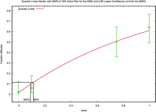
Figure 6. Fit for the Weibull model based on the hypothetical data set in Table 1.

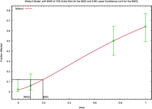
Figure 7. Fit for the Gamma model based on the hypothetical data set in Table 1.

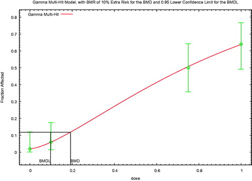
Table 2. Modeling results based on data in Table 1.

Model	Goodness of fit p value	Max. log-likelihood*	Visual fit	BMD: BMDL ratio	AIC	BMD estimate**	BMDL estimate
Quantal linear	0.53	−84.3	Acceptable	1.2	172.6	0.11	0.092
Weibull	1.0	−83.6	Good	2.0	173.2	0.20	0.098
Gamma	0.92	−83.6	Good	2.0	173.2	0.19	0.098

* The saturated model max. log-likelihood = −83.5786.

** The true BMD is 0.32.

All three models fit the data adequately with satisfactory p values, residuals, and at least acceptable visual fit. However, even though the model used to generate the underlying dose-response is determined by a Weibull function, a poorer BMD:BMDL ratio was obtained with the Weibull model than with the quantal linear or gamma models (although not by much in this example). Although the ratio is <3 for all models, this example illustrates that the BMD:BMDL ratio did not correlate with the best overall model fit; its values would not enable one to identify the correct model underlying the generation of the observations and would, in fact, suggest that the linear model was a better choice, all other parameters being equal. Likewise, this example also illustrates that the AIC is only one parameter to be used in the determination of overall model fit, since the AIC for the quantal linear model is also slightly lower than for the other two models suggesting it is also a better fitting model. However, both the ratios and the AIC’s are close enough among these 3 models to suggest that the data do not provide enough evidence, on their own, to strongly favor any one model above the others, even though the data were generated from the Weibull model. By Bayes theorem, the Weibull model is slightly more likely a posteriori, if we assume equal prior model weights.

So what does the BMD:BMDL ratio for a model indicate? Rather simply, it indicates, conditional on the model in question being correct, the degree to which the experimental design under consideration is informative about the BMD value of interest. In this example, if we had perfect knowledge that the linear model was a description of the actual dose-response,⁹ then we would infer that the experimental design provides a fairly precise estimate of the BMD, since the ratio is a value of 1.2. On the other hand, if we had perfect knowledge that either the Weibull or the Gamma models were actually a description of the true dose-response, we would have to conclude that the experimental design only allows a less precise BMD estimate (i.e. the lower confidence limit on the BMD is less close to the best estimate of the BMD). That is the combination of the experimental design (e.g. the location and spacing of the doses) and underlying true probabilities of response at those doses is not adequate for differentiating between the linear model and the Weibull model (which we used in this case to develop the actual incidence data). In other words, the underlying probabilities are not different enough to distinguish among these different models. This is not to say that there is anything inherently wrong with the standard experimental designs or the use of BMD modeling in this case. Indeed, the need to capture the uncertainty in the BMD estimate is part of the reason for using the BMDL, instead of the BMD, as the POD.

But note that these conclusions depend on having prior knowledge of the actual dose-response for the biology of the response. In both this example, and in standard BMD modeling, there is no basis for determining whether or which of those assumptions is justified, which leads to the use of multiple criteria in the judgment of model(s) most likely to best represent the underlying biological data. In fact, in this example the likelihood of obtaining the observations is almost the same for a specific linear model (background = 0.02, slope = 1, probability of the observations = 4.26E-4) and for the specified Weibull model (probability of the observations = 4.32E-4). That is why we emphasized the role of experimental design in the previous paragraph.

Thus, while the BMD:BMDL ratio provides some information on the precision of the BMD estimate, it cannot be used to evaluate the underlying assumption of model correctness to the actual (but unknown) biological dose response. Instead, the correctness or adequacy of a model needs to be evaluated using a mathematical concept of goodness of fit, such as the standard fit metrics (goodness of fit p values, residuals, visual fit, and AIC). While the value of the BMD:BMDL ratio does not correlate with any mathematical concept of goodness of fit, some risk assessors would use the BMD:BMDL ratio to give an overall sense of whether the BMDL reflects any “particular influence of the individual models” (US EPA’s statement here).

This leads to the pragmatic question of how (or whether) this particular metric can serve any meaningful role into decisions about selecting among models (and corresponding BMDL values) for use as a POD. Our analysis suggests that use of the ratio directly for choosing the best fitting model would be problematic by itself. However, this measure does inform at least in part how various models (given similar fit statistics) can describe the level of certainty in characterizing the BMD. One option for addressing this metric is to ensure that models with BMD:BMDL ratios that are large compared to other well-fitting models are closely examined with the goal of assessing the aspects of those models that result in the larger ratio. This approach can at least inform questions of model dependence and aspects of the models or data that generate a larger prediction space. Such insights can then be used as part of the weight of evidence. In the future, model averaging may be a means to reduce the “influence of any particular model,” and thus would tend to lessen the impact of any single model with a BMD:BMDL ratio that is highly different from other models. In other words, model averaging (even if the models end up with similar weights), would lessen the impact of any one model. Combining models (if the BMDs are similar) can be thought of as enriching the central tendency estimate, increasing the probability of values around the common BMD range, and, therefore, moving the tails of the distributions (i.e. the BMDLs) toward the center. A more direct approach might be to include in the model averaging some approach for weighting models such that the more certain models receive higher weights, based on both biological and mathematical aspects of uncertainty. This approach would capture uncertainty in the assessment, and avoid having the most uncertain model results drive the assessment, as may occur when simply choosing the model that results in the lowest BMDL. Thus, while there currently is no firm guidance on how to address this specific metric, close examination of the parameter can be used to inform in part BMDL selection, although it provides insights different from overall model fit.

3. Case studies

To illustrate the implications of the differences in modeling approaches and interpretation of the modeling results, we present here four case studies where different results were obtained by knowledgeable and credible scientists based on the same data sets. These case studies illustrate how the challenges and differences in perspectives and guidances can result in substantial differences in the resulting estimates of safe doses and underline the need for additional harmonization.

3.1. 3-Monochloropropane-1,2-diol (3-MCPD)– demonstrating the impact of restricting models and the use of the BMD/BMDL ratio

3-Monochloropropane-1,2-diol (3-MCPD) is a contaminant formed primarily through the refining of edible oils. Five groups of investigators (Hwang et al. 2009; Abraham et al. 2012; Rietjens et al. 2012; EFSA 2016; JECFA 2016, 2017) used the BMD approach to derive a tolerable daily intake (TDI) for 3-MCPD. In light of differences from the JECFA assessment and the updated EFSA (2017) guidance on BMD modeling, EFSA conducted an updated assessment of 3-MCPD (EFSA 2018). All of these groups based their TDIs on the same study (Cho et al. 2008), which reported kidney hyperplasia (Table 3) at a lower dose than the only other chronic study reporting non-neoplastic effect levels (Sunahara et al. 1993)¹⁰. In the one difference regarding the input data, Rietjens et al. (2012) pooled the incidence of kidney hyperplasia in males in both the Cho et al. (2008) and Sunahara et al. (1993) studies as well as the females in the Sunahara study for their analysis, because there was no significant difference in the dose-response of these groups. Despite the use of (mostly) the same input data, the resulting BMDLs identified as PODs by these five groups of investigators differ by more than 10-fold (Table 4).

Table 3. Incidence of renal hyperplasia in male rats exposed to 3-MCPD from Cho et al. (2008).

This article dose (mg/kg/d)	EFSA dose (mg/kg/d)	Number of animals	Hyperplasia incidence
0	0	50	1
1.97	2	50	11
8.27	8.3	50	21
29.5	29.5	50	36

Table 4. Basis for TDIs for 3-MCPD-induced renal hyperplasia of various investigators.

	This article	This article – model averaged	Abraham et al. (2012)	EFSA (2016)	EFSA (2018)	JECFA (2016, 2017)	Rietjens et al. (2012)	Hwang et al. (2009)
BMD (mg/kg/d)	1.2	1.5	0.92	0.54*	0.68	1.2 (1.29)¶	1.27	1.2
BMDL (mg/kg/d)	0.87	0.74‡	0.27	0.077*	0.20	0.87 (0.89)	0.72	0.87
TDI (mg/kg/d)†	9	7	2.7	0.8	2	4.0	7.0	9.0
Dataset POD	Cho et al. (2008), male only	Cho et al. (2008), male only	Cho et al. (2008), male only	Cho et al. (2008) male only	Cho et al. (2008), male only	Cho et al. (2008) male only	Cho et al. (2008) and Sunahara (1993)	Cho et al. (2008) male only
BMD model	Log-logistic (restricted)	Average of 9 models	Log-probit (unrestricted)	Gamma (unrestricted)	Model averaging	Log-logistic (restricted)	Average of 7 models	Log-logistic (restricted)
BMD/BMDL ratio	1.4	1.2	3.3	7.1	3.4	1.4	NA	1.4

NA: not applicable; POD: point of departure

* The small difference between this BMD and BMDL and that reported in Table 5 for this model is likely due to differences in rounding for the doses. See Table 3 for differences in the input doses.

† Note unit change; each BMDL has been divided by a 100-fold uncertainty factor to reflect experimental animal to human extrapolation and within human variability (10-fold each), and in the case of JEFCA, an additional 2-fold factor to reflect other data uncertainties. Hwang et al. (2009) did not develop a TDI; this value is presumed.

‡ BMDL(BCa) – BMDL based on bootstrap, corrected, and accelerated method.

¶ Second number is model averaged, for comparison purposes.

This difference in PODs, despite identical inputs, led some of us (MD, AP) to conduct an independent BMD evaluation of kidney hyperplasia found in Cho et al. (2008) and Sunahara et al. (1993). We summarize the modeling results for the former study here in comparison with others, and provide the modeling results for the Sunahara study in the Appendix. The data for renal hyperplasia in male rats from Cho et al. (2008) and Sunahara et al. (1993) were modeled using BMDS 2.601. For both data sets, several models adequately fit the data using the US EPA (2012) criteria. Male rats were more sensitive than female rats; thus male rat data were selected for the point of departure in this assessment. The BMD analysis for renal hyperplasia in male rats from Cho et al. (2008) is shown in Table 5.

Table 5. BMD results for 3-MCPD induced renal hyperplasia in male rats from Cho et al. (2008).

Model name	p value	Scaled residual nearest the BMD	Scaled residual control group	Visual fit	BMD:BMDL ratio	AIC	BMD (mg/kg/d)	BMDL (mg/kg/d)
Log-logistic (restricted)	0.61	0.90	−0.20	Good	1.4	194.8	1.2	0.87
Gamma (unrestricted)	0.92	0.0	0.0	Good	7.1	195.8	0.53	0.074
Weibull	0.81	0.0	0.0	Good	4.7	195.9	0.63	0.13
Log-logistic (unrestricted)	0.57	0.0	0.0	Good	3.7	196.1	0.83	0.22
Log-probit (unrestricted)	0.54	0.0	0.0	Good	3.3	196.2	0.92	0.27
Multistage (unrestricted)	0.25	1.0	−0.20	Good	1.4	197.1	1.3	0.90
Gamma (restricted)	0.07†	1.6	−1.0	Poor	1.3	199.0	2.1	1.7
Multistage (restricted)	0.07	1.6	−1.0	Poor	1.3	199.0	2.1	1.7
Quantal-linear	0.07	1.6	−1.0	Poor	1.3	199.0	2.1	1.7
Log-probit*	0.01	2.0	−2.0	Poor	1.3	204.8	4.0	3.0
Probit	0.00	2.1	−2.5	Poor	1.2	208.4	5.4	4.5
Logistic	0.00	2.1	−2.6	Poor	1.2	209.0	5.6	4.6

*A restricted version of the Log-probit model is not available.

†Models with data in italics were eliminated due to unacceptable fit.

Using the US EPA approach, the first step in identifying a POD is to eliminate models with unacceptable fit, based on the goodness of fit p values, scaled residuals, and visual fit. This eliminates the models show in italics in Table 5. Applying the EFSA (2017) guidance would result in the same narrowed group of models, based on the criterion of focusing on models with an AIC within two units of the lowest model AIC (This narrowing is done according to the EFSA guidance only if model averaging software is not available).

The remainder of the model selection approach illustrates how different approaches can result in substantially different PODs. Abraham et al. (2012) applied the EFSA (2009) guidance, and identified a BMDL₁₀ of 0.27 mg/kg/d (based on the Log-probit model), because it was the lowest BMDL of the models with acceptable fit and without infinite low-dose slope (i.e. focusing on the restricted models). Consistent with the EFSA (2017) guidance, Rietjens et al. (2012) did not apply any model constraints/restrictions (aside from requiring that the shape parameters be positive), and applied model averaging using the method of Wheeler and Bailer (2008). We found similar results for model averaging, using only the Cho et al. (2008) data, and applying model averaging using the same method¹¹. EFSA (2016) did not use model averaging, and used the lowest BMDL₁₀ of all of the models with acceptable fit, including the unrestricted models; this approach is also consistent with the EFSA (2017) guidance. EFSA (2018) applied model averaging and obtained a BMDL₁₀ of 0.20 mg/kg/d, a value somewhat lower than that from the other assessments using modeling averaging. EFSA (2018) attributed the difference from the JECFA model-averaged result to JECFA applying additional parameter constraints (model restriction) that were not applied by EFSA¹².

The remaining three assessments (Hwang et al. 2009; JECFA 2016, this article) all identified a BMDL₁₀ of 0.87 mg/kg/d, based on the restricted log-logistic model, although there were some differences in the rationale. JECFA (2016) chose the results from the log-logistic model as the “lowest BMDL,” apparently focusing only on the restricted models when there was an option for restricting. Hwang et al. (2009) chose this model based on it having the lowest AIC (according to US EPA guidance), with visual confirmation of the goodness of fit. The assessment for this article considered the various measures of fit, as well as the BMD:BMDL ratio. Rather than simply preferring the restricted models over the unrestricted models, it was noted that the lowest BMDL found in Table 5, that from the Gamma (unrestricted) model has a BMD/BMDL ratio much greater than 2, and that this large ratio of 7.1 provides much of the explanation of why the BMDL is the lowest for this model. In other words, the BMDs of the various models differ by a factor of 2.2 or less, whereas the BMDLs are up to 12-fold different. In contrast to the large BMD:BMDL ratio for the unrestricted Gamma model, the BMD:BMDL ratio for the restricted log-logistic model is 1.4. Figures 8 and 9 present the model graphs for the Log-logistic (restricted) and Gamma (unrestricted) model, respectively.

Figure 8. BMD log-logistic (restricted) graph for 3-MCPD induced renal hyperplasia in male rats from Cho et al. (2008).

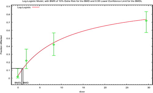
Figure 9. BMD Gamma (unrestricted) graph for 3-MCPD induced renal hyperplasia in male rats from Cho et al. (2008).

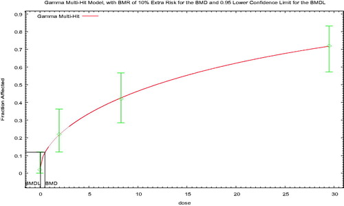
As discussed in Section 2.8, the BMD:BMDL ratio is used by some assessors as part of the second tier of considerations in the choice of the best fitting model. Using this ratio as a criterion in the case of models with otherwise similar fits would also be a reason to exclude the unrestricted Gamma model, even if one were including unrestricted models.

Thus, the key issue illustrated by this example is whether one should first focus on the “restricted” models (if adequate fit can be obtained with those models), or whether one should consider the restricted and unrestricted model results together, as discussed above in Section 2.5. This is an area of clear disagreement, where US EPA (2012) and EFSA (2017) present somewhat different perspectives (although it is noted that one of the authors of the Slob and Setzer paper is from US EPA). Even when model averaging is applied, the issue of model restriction affects the result, although the impact is smaller. Clearly, this is an area where additional discussion and harmonization would be of value, given the substantial impact on the final choice of BMDL. In addition, consideration of the BMD:BMDL ratio as part of the decision criteria in choosing the best overall model would have the same impact in this case as excluding the unrestricted models. This is often the case, since the unrestricted models often have wider confidence limits. Finally, the use of model averaging, as was applied by Rietjens et al. (2012), will aid in avoiding disagreements in the future on the choice of a single best overall model, although issues remain in determining the appropriate weighting approach and whether to include unrestricted models in the averaging.

3.2. 5-Hydroxymethylfurfural (HMF) – use of visual fit, AIC, and residuals

5-Hydroxymethylfurfural (HMF) is a flavoring agent that has been evaluated by the European Food Safety Authority (EFSA 2011). This authority developed a BMD of 29.5 mg/kg/d and its lower limit (BMDL) of 20.2 mg/kg/d based on renal tubule epithelium cytoplasmic alterations in male mice observed in a 90-day oral gavage study of NTP (2010) as shown in Table 6. EFSA conducted BMD modeling with the PROAST version 27.4 (RIVM, Bilthoven, The Netherlands) statistical package utilizing all PROAST models (i.e. the “standard dichotomous models” of BMDS). EFSA concluded that all models provided an acceptable fit to the data; therefore, the lowest BMDL was selected as the point of departure, consistent with the EFSA (2009) and (2017) guidance. Figure 10 shows the plot of the chosen model.

Figure 10. EFSA One-stage BMD model plot for cytoplasmic alterations in the renal proximal tubule epithelium in male mice due to 5-HMF.

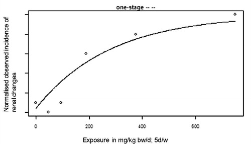
Table 6. HMF-induced renal tubule cytoplasmic alterations in male mice after 90-d oral gavage.

HMF (mg/kg/d)	Number of animals	Renal tubule cytoplasmic alteration incidence
0	10	1
47	10	0
94	10	1
188	10	6

An independent assessment by two of the authors of this article (AP, MD) repeated the modeling conducted by EFSA, using the standard dichotomous models available in US EPA’s BMDS version 2.601 (EPA, Washington, DC) (Rodriguez et al. 2016). This assessment obtained comparable BMDs and BMDLs to those reported by EFSA (Table 7). However, based on the “holistic” approach to model selection described in Section 2.6.3, Rodriguez et al. (2016) came to a different conclusion from EFSA regarding the appropriate choice of BMDL.

Table 7. BMD modeling results for 5-HMF induced renal tubule cytoplasmic alterations in male mice.

Model name	p Value	Scaled residual at dose	Scaled residual at zero	Visual fit	Ratio BMD:BMDL	AIC	BMD (mg/kg/d)	BMDL (mg/kg/d)
Multistage-3	0.50	−0.51	0.727	Good	2.4	44.5	87.4	36.1
Log-probit	0.50	−0.339	0.78	Good	1.7	45.3	96.0	57.4
Probit	0.41	−0.606	0.674	Acceptable	1.4	45.3	79.6	54.9
Logistic	0.41	−0.583	0.553	Acceptable	1.5	45.4	84.5	57.1
Log-logistic	0.44	−0.342	0.79	Good	1.7	45.7	95.9	55.5
Gamma	0.41	−0.422	0.753	Good	2.0	45.8	92.6	47.1
Weibull	0.35	−0.554	0.747	Acceptable	2.1	46.5	84.3	40.7
Quantal-linear	0.17	−1.533	0.909	Poor	1.5	49.8	29.5	20.2
Multistage-1	0.17	−1.533	0.909	Poor	1.5	49.8	29.5	20.2
Multistage-cancer*	0.17	−1.533	0.909	Poor	1.5	49.8	29.5	20.2
Multistage-2	0.00	0	0	NA	1.0	35 512.5	0.0	0.0

NA: not applicable

* This model is similar to the one-stage model of EFSA as shown in Figure 10.

Specifically, the first criterion of p values less than 0.1 allowed one model (i.e. multistage-2) to be rejected. All other models adequately fit the data based on this goodness of fit p values. Two models were rejected based on poor visual fit, specifically, the one-stage multistage–Cancer (which is the same as the multi-stage cancer model and similar to the model chosen by EFSA) and quantal-linear. Seven models gave acceptable or good visual fits, but the fits of the log-logistic, Gamma, multistage 3, and log-probit models were judged to be better than those of the Weibull, Probit, and logistic models. All four of the better-fitting models had good residuals (values well less than an absolute value of 2) and AICs within 2 units; the BMD:BMDL ratios were also 3 or less for all four models, and less than 2 for several. The log-probit visual fit is shown in Figure 11 and the multi-stage 3 visual fit is shown in Figure 12. Rodriguez et al. (2016) chose the log-probit model based on the slightly lower scaled residual and lower BMD:BMDL ratio. The BMD and BMDL for this model were 96 and 57 mg/kg/d, respectively (Table 7). The model with the best (lowest) AIC was the multistage 3, with a BMD and BMDL of 87 and 36 mg/kg/day, respectively. Using the US EPA (2012) guidance, the multistage 3 model would be chosen. However, it is noted that all of the models with acceptable or better fits had AIC values within 2 of the model with the lowest AIC. It is also noted that, unlike the MCPD example, the differences between the BMD:BMDL ratios for the log-probit and multistage 3 models is relatively small. Thus, yet another alternative would be to average the BMDLs from the four best-fitting models, consistent with an option provided by US EPA (2012); this would result in a very slight decrease in the BMDL, to 49 mg/kg/d. And finally, using model averaging would avoid the need to choose a single model.

Figure 11. BMD log-probit plot for cytoplasmic alterations in the renal proximal tubule epithelium in male mice due to 5-HMF.

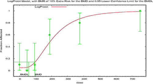
Figure 12. BMD multistage-3 plot for cytoplasmic alterations in the renal proximal tubule epithelium in male mice due to 5-HMF.

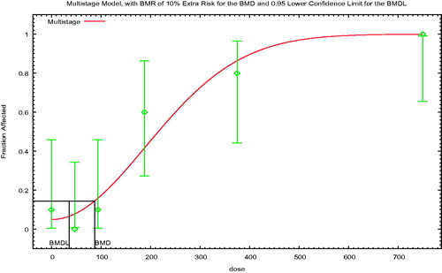
This dataset highlights some of the strengths and pitfalls of focusing on visual fit and attempting to choose the best model based on consideration of multiple fit criteria, as well as the importance of recognizing the underlying assumptions that may affect the judgment of fit. Compare Figures 10–12, reflecting in concept¹³ the models chosen by EFSA (2011), Rodriguez et al. (2016), and the model with the lowest AIC, respectively. The multistage-1 model appears to miss the first two non-zero data points, although the curve is within the confidence limits. In contrast, the Log-probit and multistage-3 models do a good job of estimating the control response and the first two nonzero data points. Of particular interest with regard to the visual fit is the difference in curvature between the multistage-1 model and the other two models. The multistage-1 model is concave downward, with the curve essentially splitting the difference between the response at the control dose and the two lowest non-zero doses. In contrast, the other two models have the S-shaped curve often seen with dose–response curves, with an initial shallow slope, followed by a more rapid increase. Thus, while a mathematician might appropriately say that all three curves are consistent with the data, a biologist might prefer the log-probit or multistage-3 curves as better reflecting the expected low–dose curve shape. Decisions about the expected shape of the curve in this region are particularly important, since this is the region of the BMD and BMDL.

This difference between the models is also reflected in the scaled residuals (which are part of the US EPA criteria for acceptance, but not those of EFSA). None of the models would be considered unacceptable based on the scaled residuals, since US EPA considers models unacceptable only if the absolute value of the scaled residual is >2. However, a holistic approach would tend to discount the multistage-1 model based on the substantially larger scaled residual. The scaled residuals are comparable for the multistage-3 and log-probit models, and thus do not aid in distinguishing these two models. Finally, it is noted that, based on the AIC, there is a clear preference according to US EPA’s guidance for the multistage-3 and log-probit models over the multistage-1 cancer model, since the AIC for the multistage-1 model is more than 5 higher than that for the other two models. Although EFSA (2017) does not recommend choosing the model based on the AIC, it does recommend that if model averaging software is not available, that models with AICs that differ from the lowest AIC by more than two be excluded from consideration for the POD. The multistage cancer model would also be excluded based on this criterion.

Thus, based on our understanding of the current EFSA guidance, it appears that the model chosen by EFSA (2011) would likely not be chosen by EFSA according to its current 2017 guidance, although a definitive determination is not fully possible, due to the absence of several key parameters in the EFSA (2011) report. It appears likely that EFSA would choose the multistage-3 model (BMDL of 36 mg/kg/day), based on the choice of the lowest BMDL among the models with an AIC within 2 of the lowest AIC.

3.3. Nickel – use of models for nested data

The BMDS software developed by the US EPA includes models designed for nested dichotomous results from developmental toxicity studies, in addition to the models for standard continuous and dichotomous endpoints. As an illustration of the impact of using the models for nested data rather than the standard dichotomous models, consider the development of a chronic oral safe dose for nickel. EFSA (2015) and (Haber et al. 2017) both recently assessed the nickel database. Both assessments chose as a critical effect post-implantation loss in a 2-generation study and the related range-finding study (SLI 2000a, 2000b)¹⁴. EFSA used the standard dichotomous models to model the incidence of litters with post-implantation loss from the combined dose-range finding study and the first generation of the 2-generation study. We have recreated the EFSA results (Table H5 of that report) for this manuscript, which are presented in Table 8¹⁵.

Table 8. BMD analysis of the incidence of litters with post-implantation loss per treatment group from SLI (2000a, 2000b), based on approach of EFSA (2015); doses in mg Ni/kg-day.

Model name	p Value	Scaled residual	Visual fit	Ratio D/L	AIC	BMD	BMDL
Gamma	0.67	−0.049	Acceptable	1.7	211.5	0.50	0.29
Logistic	0.68	−0.035	Acceptable	1.6	211.3	0.64	0.41
Log-logistic	0.40	0.43	Acceptable	21	214.4	3.0	0.14
Log-probit	0.39	0.10	Acceptable	5.9	214.4	3.3	0.57
Multistage-1	0.67	−0.049	Acceptable	1.7	211.5	0.50	0.29
Multistage-2	0.57	−0.043	Acceptable	2.5	213.1	0.76	0.30*
Multistage-3	0.60	−0.065	Acceptable	2.5	212.8	0.76	0.31
Probit	0.69	−0.040	Acceptable	1.5	211.1	0.69	0.45
Weibull	0.54	−0.024	Acceptable	2.3	213.5	0.66	0.29
Quantal-linear	0.67	−0.049	Acceptable	1.7	211.5	0.50	0.29

* Model that was the basis for the EFSA assessment¹⁵.

Haber et al. (2017) used the models for nested dichotomous data to evaluate the same data sets. The first step was to evaluate which data sets could be combined appropriately. Acceptable model fits were obtained for the combined datasets of the dose-range finding study (1-gen) combined with either the first (2-gen-1) or second (2-gen-2) generation of the 2-generation study, but were not obtained when both the 2-gen-1 and 2-gen-2 data were included. See Table 9 and note that, for these developmental models, a goodness of fit p value of 0.05 or better is considered acceptable.

Table 9. Goodness of fit p values for data set combinations for post-implantation loss from SLI (2000a, 2000b) and Haber et al. (2017)*.

	Data set combinations: GoF p values
Model	1-gen + 2-gen-1	1-gen + 2-gen-2	2-gen-1 + 2-gen-2	All 3
NLN	0.08	0.11	0.03	0.02
NCTR	0.08	0.11	0.03	0.02

* Model forms with an intra-litter (IC) correlation, but not a litter-specific correlate (LSC) had the best fit. Because the NCTR and RVR models are the same when LSC is excluded from those models, results are presented for the NLN and NCTR models only.

Results of the modeling by Haber et al. (2017) are shown in Table 10, including results for a BMR of 10% (consistent with standard US EPA practice), as well as results based on a 5% BMR. The BMDL05 was used due to the greater sensitivity of the nested study design (US EPA 2012), and consistent with the results of (Allen et al. 1994a, 1994b) analyzing the comparability of NOAELs and BMDLs for a large database of developmental toxicity studies using models for nested data, as done here.

Table 10. BMD and BMDL estimates for post-implantation loss, combined data sets (mg Ni/kg/d) from SLI (2000a, 2000b) and Haber et al. (2017).

		Data set combinations: GoF p values
BMR		1-gen +2-gen-1 (A)		1-gen +2-gen-2 (B)		2-gen-1 + 2-gen-2* (C)		All 3* (D)
(extra risk)	Model	BMD	BMDL	BMD	BMDL	BMD	BMDL	BMD	BMDL
10%	NLN	6.3	3.9	6.4	4.2	4.9	2.3	6.2	4.1
	NCTR	6.7	3.3	6.6	3.3	4.8	2.4	6.4	3.2
5%	NLN	3.0	1.8*	3.1	2.0*	2.3	1.3	2.9	1.9
	NCTR	3.2	1.6*	3.2	1.6*	2.3	1.2	3.1	1.6

BMDL values represent 95% lower bounds on the corresponding BMD.

* Models including both 2-gen-1 and 2-gen-2 (whether or not the 1-gen is included) are given lower credence based on p values of 0.03 and 0.02, respectively, from Table 9. Model results used for the final calculation of the point of departure are bolded.

Comparing the results from the two methods in Tables 8 and 10 (bolded numbers), the final BMDLs differ by a factor of more than five: 0.28 or 0.30 mg/kg/d using the standard dichotomous models from Table 8, and 1.6–2.0 using the models for the nested data from Table 10. This difference occurs even though the BMR used for the standard dichotomous modeling was 10%, while a 5% BMR was used for the models for nested data. The difference is more than ten-fold if a BMR of 10% were chosen for these nested data as also shown in Table 10. Use of the models for nested data in this case provides a better estimate of the BMDL, by using more of the data, and is health-protective even though the BMDL is higher than that calculated using the standard models. It is also noted that methods are now available for using the summary data on a per litter basis, but appropriately accounting for clustering (Fox et al. 2017). If the analyses are conducted without accounting for the clustering, the variances are overestimated.

3.4. Perchlorate – choice of the BMR

This case study illustrates the use of different definitions of adversity and associated differences in the critical effect, in the development of safe doses. This issue is a common one in toxicological risk assessment, regardless of whether safe doses are based on the NOAEL/LOAEL approach or on BMD modeling. Indeed, determining whether the effects seen at a specific dose are adverse is one of the more challenging aspects of toxicological risk assessment and, in our experience, one of the prime sources of controversy in the development of risk values. The perchlorate case study illustrates that, even though BMD modeling is fundamentally a mathematical curve-fitting exercise, biological considerations and biological interpretation still play a crucial role in the identification of the appropriate endpoint(s) to model and the choice of the BMR; differences in the biological interpretation can thus have a substantial impact on the final result.

Perchlorate is a drug, a rocket fuel ingredient, and a natural part of desert environments. It is also found as an environmental contaminant in the soils of certain areas and in the food and drinking water of several locations. Several groups have established the safe dose for perchlorate, including but not limited to (Strawson et al. 2004) with a value of 0.002 mg/kg/d, the (NRC 2005), and (US EPA 2005) with identical values of 0.0007 mg/kg/d (JECFA 2011) with a value of 0.01 mg/kg/d and (EFSA 2014) with a value of 0.0003 mg/kg/d. These values differ by about 30-fold. Importantly, each of these groups used the same basic information to determine their safe doses.

The oldest of these safe doses, those of Strawson et al. (2004), NRC (2005) and US EPA (2005), were based on NOAELs for different critical effects. Strawson et al. (2004) based their NOAEL on serum T4 decrease in children from an epidemiology study of three different populations in Chile by Crump et al. (2000), while (NRC 2005) and (US EPA 2005) based their NOAEL on inhibition of iodide uptake in adults from a study by Greer et al. (2002), where 16 males and 21 females were given perchlorate in drinking-water at doses of 0.007, 0.02, 0.1, or 0.5 mg/kg bw per day for 14 d, respectively. The uptake of iodide into the thyroid was measured at baseline before administration of perchlorate and on days 2 and 14 of administration at both 8 and 24 h after administration of radiolabeled iodine. The NOAELs were nearly identical in these two studies – 0.006 mg/kg/d for children from Crump et al. (2000) and 0.007 mg/kg/d for adults from Greer et al. (2002). The difference in safe doses was due to the choice of uncertainty factor – 3-fold in the case of Strawson et al. (2004) and 10-fold in the case of NRC and US EPA.

JECFA (2011) used the same human clinical study as (NRC 2005) and (US EPA 2005), that by (Greer et al. 2002). Like (NRC 2005) and (US EPA 2005), JECFA (2011) considered the critical effect for perchlorate to be its ability to competitively inhibit uptake of iodide by the thyroid gland, potentially causing hypothyroidism. JECFA used BMD modeling and judged that a BMR of 50% inhibition of iodide uptake from a clinical study in healthy adults was appropriate, as data from healthy adults following both short-term and chronic exposure to perchlorate have shown that such a level of inhibition is not associated with any changes in TSH or thyroid hormone levels. A BMDL₅₀ of 0.11 mg/kg/d followed. Because perchlorate was rapidly cleared from the body, JECFA (2011) concluded that it was not necessary to apply an uncertainty factor to account for the short duration of the pivotal study, as there were efficient homeostatic mechanisms to cope with short-term and long-term inhibition of iodide uptake, up to (at least) 50% inhibition in healthy children and adults. A further reason for the absence of the duration uncertainty factor was based on the observation of at least a 4-fold margin between the value of the BMDL₅₀ and the dose of >0.4 mg/kg/bw per day of sustained exposure necessary to trigger hypothyroidism in normal adults (Greer et al. 2002). JECFA (2011) applied a 10-fold factor to the BMDL₅₀ to account for sensitive population subgroups, resulting in a safe dose of 0.01 mg/kg/d.

In contrast to JEFCA (2011), EFSA (2014), who also used BMD modeling, selected a BMR of 5% thyroid iodide uptake inhibition from the same study of Greer et al. (2002), for the establishment of its tolerable daily intake (TDI) for perchlorate. This resulted in a BMDL of 0.0012 mg/kg/d. EFSA’s justification for a BMR of a 5% inhibition of iodide uptake is that this would not lead to adverse effects in any subgroup of the population, and because of this choice EFSA did not consider that an uncertainty factor was necessary for intraspecies differences in toxicodynamics. However, EFSA judged that an uncertainty factor of 4 was needed for intraspecies differences in toxicokinetics, since PBPK modeling had shown that the degree of inhibition of iodide uptake is at most 4-fold higher in subgroups, such as pregnant women, fetuses, lactating women, neonates, and children than in non-pregnant adults (i.e. 1.9% instead of 0.6% at a dose of 0.001 mg/kg/d and 17% instead of 4% at a dose of 0.01 mg/kg/d)¹⁶. Additionally, EFSA (2014) did not judge that an uncertainty factor to account for the short-term exposure duration was necessary, because of perchlorate’s short serum half-life (mean of 8.1 h in humans). The resulting TDI was 0.0003 mg/kg/d.

These differing safe doses are based on different interpretations of the appropriate BMR for the inhibition of iodide uptake, as well as differences in the identification of the critical effect, whether iodide inhibition or thyroid hormone disturbance or something else. These differences are shown conceptually in Figure 13 from (NRC 2005). Additional data in humans by Téllez et al. (2005) and BBDR modeling by Schlosser et al. (2016) is leading to new ways to investigate the safe dose for perchlorate. This newer work is focused on the lower serum levels of T4 as the critical effect and pregnant mothers, fetuses, or newborns as the sensitive population.

Figure 13. The NRC (2005) description of effects from perchlorate exposure. Note that inhibition of iodide uptake is three steps before the first adverse effect (hypothyroidism). Redrawn from Figure 5-2 of NRC (2005).

4. Discussion and conclusions

BMD modeling is now generally accepted as the best practice for determining the point of departure for most risk assessments. Key advantages include the fact that the modeling incorporates all of the data for a particular effect from a particular experiment, increased consistency in comparing results from different studies, and better accounting for statistical uncertainties. Despite these strong advantages, disagreements remain as to several specific aspects of the modeling, particularly with regard to how the models reflect data and modeling uncertainty, and the relative weighting of biological and mathematical considerations. In particular, there are some key differences between the two published guidance documents for BMD modeling, from the US EPA (2012) and EFSA (2017). This article has attempted to identify areas where consensus exists, areas where different perspectives exist, and opportunities for additional research.

Throughout this article, we have highlighted the importance of bringing a full biological and mathematical understanding to the analysis. It is important to be consistent with guidance, but most guidance includes a number of nuances that should be considered in evaluating the data. These guidances also allow for weighing these nuances in making judgments on modeling results. Understanding the reasons for obtaining different results is important in understanding how to interpret them. Such interpretations require consideration of the available mode of action (MOA) information, the broader understanding of how the chemical acts and the biology of dose-response, study limitations, and a statistical understanding of confidence limits. Using simpler decision flows to improve consistency is important, but consistency should not be prioritized over biological plausibility. Although a MOA understanding is not necessary for conducting BMD modeling, BMD modeling can be a useful tool for evaluating MOA, particularly in applying the key events dose–response framework (KEDRF) (Simon et al. 2014). Modeling key events (KEs) along a hypothesized MOA pathway allows one to evaluate the hypothesized progression and relative order of the KEs along a dose and time continuum.

One of the recurrent themes of the article was recognizing how different results and recommendations can result from different perspectives, or where pragmatic considerations may necessitate the use of a less than ideal approach. A number of situations were identified where biologically focused assessors may prefer to use a NOAEL approach or a specific model based on pragmatic or biological considerations, while mathematically focused assessors may prefer BMD modeling and model selection based on statistical metrics.

In identifying the BMR for continuous data in cases when there is no consensus as to the degree of change that is adverse, EFSA (2017) recommends a default of a 5% change in the mean response, while US EPA (2012) recommends a BMR corresponding to a change in the control mean response of one control SD. These differences reflect differences in concerns about uncertainties. In considering the alternative approaches, US EPA (2012) expresses concern about the potential for different degrees of response being associated with the same percent change for different endpoints, while EFSA (2017) expresses concern that defining the BMR in terms of the control variability results in the BMD varying with study-specific factors.

Differences in perspective and focus were also evident in the case studies. The 3-MCPD case study illustrated the impact of restricting models and of considering the BMD:BMDL ratio. A key difference between the US EPA (2012) and EFSA (2017) guidance is in their recommendations regarding model restriction, and this issue will be discussed in some detail in the upcoming WHO paper. The 5-HMF case study illustrated how biological considerations may affect the choice of model. For two models with equivalent statistical fit (based on all statistical parameters), biologists may prefer models resulting in S-shaped curves over models resulting in linear curves or curves that are concave downwards, while mathematicians might not distinguish among the curves. Biologists and mathematicians may also differ in their assessment of the potential for rigorously evaluating visual fit. In principle, as assessors further develop statistical tools that weigh additional local fit considerations (such as local scaled residuals) the differences between visual fit and statistical fit could decrease.

The nickel and perchlorate case studies illustrated additional aspects related to biological considerations. The nickel case study highlighted the impact of using models specifically designed for nested developmental toxicity data, compared with modeling average results. The perchlorate case study illustrates the use of different definitions of adversity and associated differences in the critical effect, an issue that is not limited to BMD modeling.

Several of these issues related to model choice are likely to be reduced by the adoption of model averaging. However, in some senses, adoption of model averaging merely moves the place at which some issues are considered. Current model averaging methods use basic measures of fit (e.g. AIC) for weighting of different models, but it would be useful to be able to incorporate into the weighting biological considerations, including measures related to fit in the low-dose region and to model curvature.

This article has also identified areas for additional research, in addition to issues relating to model fit and model choice. In particular, more research is needed on the quantitative implications of the interaction between the BMR and uncertainty factors, particularly for epidemiology data. This interaction is important in understanding how to apply the US EPA (2005) recommendation to use the lowest POD adequately supported by the data, while avoiding having more sensitive studies automatically and inappropriately resulting in lower “safe dose” estimates.

Overall, this article has identified areas of consensus and sources and areas of disagreement related to BMD modeling. An understanding of different approaches and the reasons for those differences is a key step in the harmonization of methods. It is important to involve experts in both biology and mathematics in considering how to best approach the differences and move the field of risk assessment forward.

Declaration of interest

LTH, AP, MJV, and AM are employed by the University of Cincinnati (UC) and are part of the Risk Science Center (RSC) within the College of Medicine. The RSC is dedicated to scientific collaboration and transparency in support of public health protection. For this specific project, financial support was received from the Grocery Manufacturers Association, the Institute of Shortening and Edible Oils, the EU Vegetable Oil & Proteinmeal Industry, the Infant Nutrition Council of America, FoodDrink Europe, and the International Technical Caramel Association. MLD was a University of Cincinnati employee during his authorship of this article and was an employee of the US EPA when it was resubmitted. Contributions made by MLD during his employment by the US EPA were outside of his role as an EPA employee, and were limited to comments on the section on the BMD:BMDL ratio. BCA is an independent consultant specializing in dose–response models and quantitative risk assessment, and he received an honorarium as a subcontractor to UC for his contributions to the article. BCA has been a subcontractor since 2006 to Lockheed Martin and CSRA (an IT services company that provides support to EPA for its BMDS software), participating in work for EPA to maintain, update, and expand EPA’s benchmark dose software packages, BMDS, and CatReg. He has performed BMD analyses for 3 M, the Hamner Institute, ICF International, and Ramboll-Environ, roughly at times overlapping with the development of the manuscript. RCH is affiliated with Emory University as an Adjunct Professor, but contributed to the manuscript as an independent contractor, and received an honorarium as a subcontractor to UC. He has no relationship with any other funding entities. He has no business relationship with any developers of statistical software or with any of the sponsoring companies. ARB was employed by Imperial College London, where he was involved in academic research and teaching in the fields of biomedicine and toxicology until he retired in June 2017. He is currently employed 4 h per week by the College to work on an EU Horizon 2020 project (EuroMix). His contribution does directly involve BMD analysis. He has no other employment. He has received research funding from the Food Standards Agency of the United Kingdom for work that in part involved BMD modeling. He is or has collaborated on a number of activities on benchmark dose modeling through FAO/WHO JECFA, FAO/WHO JMPR, WHO-IPCS, EFSA, ILSI HESI, ILSI Europe, ILSI Research Foundation, and United Kingdom COT. None of these collaborative activities was remunerated and no research funding was received. He consulted for Coca-Cola on the safety of certain food additives, from 2012 to 2014. This work did not involve benchmark dose modeling or any other form of dose–response analysis. ARB received no funding in cash or kind for his contribution to this manuscript.

This manuscript grew out of several case studies that were individually funded, but highlighted the need for a peer-reviewed manuscript addressing the broader underlying issues that arose in the case studies. The initial case study on 3-MCPD was conducted by MLD and AP with funding from Abbott Nutrition and the Grocery Manufacturers Association (GMA). The initial case study on 5-hydroxymethylfurfural (HMF) was conducted by MLD and AP with funding from the Coca-Cola Company, and was presented as a poster at the Society of Toxicology annual meeting in 2016. The initial case study on nickel was conducted by LTH, MJV, and BCA, with funding from NiPERA, Inc, and was published as a peer-reviewed manuscript in 2017. LTH and MJV have also received funding from NiPERA, Inc. for several other projects, including review of a research plan (LTH) and a manuscript reviewing and reevaluating historical nickel exposures among workers in nickel-producing and nickel-using industries (MJV). MLD has worked on perchlorate since 1995. Prior work on perchlorate informed the text in the manuscript, and was funded by the Perchlorate Study Group (PSG), supplemented by additional tasks for Kerr-McGee Chemical Corporation and Aerojet, but he has not done any paid work on perchlorate assessment since 2006. This prior work resulted in several publications in peer-reviewed journals that were funded by Toxicology Excellence for Risk Assessment. MLD also peer reviewed an EPA position document on perchlorate in 2016 paid for by the American Water Works Association. The work on 3-MCPD and nickel also resulted in the submittal of comments to EFSA on the respective EFSA assessments, funded by the respective sponsors. In addition, MLD and AP submitted comments on the draft EFSA revisions to its BMD modeling guidelines, funded by GMA. The sponsors of the manuscript were provided the opportunity to review the initial submitted draft of this manuscript. The sponsor comments were limited to removing one of the original case studies and editorial comments. After receiving reviewer comments, the manuscript was substantially revised, and the sponsors were not provided the opportunity to review the revised text prior to re-submittal. None of the authors have during the past five years, appeared in any legal or regulatory proceedings relative to the contents of the article. The views expressed in this article are solely those of the authors and may not necessarily represent those of the sponsoring organizations.

Acknowledgments

Technical assistance from Casey Allen is gratefully acknowledged. We thank Jeff Gift and Allen Davis of the US EPA for taking the time to explain current EPA thinking and approaches. We also gratefully acknowledge the many useful comments from five anonymous reviewers, selected by the Editor, which substantially enhanced this article.

Notes

Notes

1 Evolution in terminology has added confusion. Early papers by Crump, Allen and others used the term maximum likelihood estimate (MLE) to refer to the central tendency/best estimate, and the term BMD to refer to the lower bound. Current practice is to use BMD for the central tendency and BMDL for the lower bound. In addition, the term BMD is sometimes used generically to refer to the results of the modeling.

2 The critical effect is the first relevant effect stated to be adverse or its known and immediate precursor, that occurs in the dose scale in humans or the most relevant experimental animal species, or in the most sensitive experimental animal species, if the former is unknown. Protecting against the critical effect is assumed to protect against other adverse effects, especially those of greater severity.

3 Chiu and Slob (2015) noted that dichotomous data have an underlying continuous endpoint. For example a pathologist may evaluate the number of dead cells in the liver in order to determine whether the animal is affected with liver necrosis, and at what severity. Consideration of the underlying continuous distributions is beyond the scope of this article.

4 With modern data-handling programs for good laboratory practice (GLP) studies, it is often possible to electronically extract the needed data.

5 Categorical regression (Dourson et al. 1997; Guth et al. 1997; Haber et al. 2001) allows one to look at the combined dose-response from related endpoints, among other applications, but has other drawbacks beyond the scope of this article.

6 Note that, for the same data set, a lower BMR will result in a lower BMDL, but the BMDL may not necessarily be lower than what would have been determined in a hypothetical study with the same response incidence but a smaller sample size. This is because of the tighter confidence limits presumably associated with the larger sample size. However, this hypothetical example presumes a lower BMDL.

7 US EPA (2012) does not recommend specific models, but US EPA practice can be inferred based on the models in BMDS.

8 One of us (MD) interprets the phrase in question as being addressed by the BMD:BMDL ratio. (Others of the authors interpret the phase as merely rewording the first part of the sentence.) Based on the former interpretation, the argument is that large BMD:BMDL ratios reflect greater model uncertainty, and so models with larger ratios should not be used, other criteria being equal. However, as described further in the remainder of this section, although the magnitude of the ratio is a measure of the uncertainty in the BMD estimate, a mathematician would consider it to be more a reflection of the uncertainty related to the data than the uncertainty specific to the model.

9 A linear model with background = 0.02 and slope = 1, would be almost as likely as the true Weibull model to generate the observed responses shown. The BMD for that model is approximately 0.11.

10 EFSA (2018) noted that the BMDL for sperm effects in a 13-week study was slightly higher than that for the kidney effects.

11 Modeling conducted using the Model Averaging for Dichotomous Response Benchmark Dose (MADr-BMD) software, available at https://www.epa.gov/tsca-screening-tools/model-averaging-dichotomous-response-benchmark-dose-madr-bmd-tool. All models were restricted, and the model weighting was based on the AIC.

12 The JECFA model averaging also used the Wheeler and Bailer software, including all of the (restricted) models except the quantal-quadratic model, and conducting the averaging using the Bayesian information criterion (BIC). EFSA used the R package proast 64.9 to do the modeling, using the default set of fitted models, as specified by EFSA (2017).

13 EFSA used the one stage model, but did not include confidence limits on the graph. To illustrate the points being addressed here, the graph being shown is for the Multistage Cancer model of BMDS. This model is very similar to the one stage model, but somewhat different BMD and BMDL were obtained from that of EFSA (2011), and so it is recognized that the analogy is not perfect.

14 This is an unpublished GLP study.

15 The re-created results are shown rather than EFSA’s, in order to provide the standard fit information, which was not fully detailed in the EFSA report. In addition, EFSA ran the restricted model only when the unrestricted model failed, while we followed EPA approach of running the restricted models when available, and using the unrestricted model if the restricted model failed, a situation that did not occur for this dataset. This issue of restriction is the reason why this table shows 0.30 for the BMDL for the multistage-2 model, while EFSA identified a BMDL of 0.28. There were also several other minor differences between our results, particularly for the p value, but these differences do not affect the overall conclusions.

16 Note that this quantitative comparison is not consistent with the approach recommended for CSAFs by IPCS (2005). Instead of comparing the response at a specified dose, IPCS defines the CSAF as the ratio of doses (e.g. BMDs) that result in a defined response (e.g. BMRs).

Appendix

The appendix: 3-Monochloropropane-1,2-diol (3-MCPD) – Results of modeling the Sunahara et al. (1993) data

The results from modeling the Sunahara et al. (1993) data are shown in Appendix Table 1. They show that BMDLs obtained from male rats in Sunahara et al. (1993) values were slightly higher than those found in Cho et al. (2008) as shown in Table 4 of the main text, but were otherwise supportive.

Appendix Table 1. BMDS results for renal hyperplasia in male rats from Sunahara et al. (1993).

Model name	p Value	Scaled residual nearest the BMD	Scaled residual control group	Visual fit	BMD/BMDL ratio	AIC	BMD	BMDL
Gamma (restricted)	0.63	0.1	−0.4	Good	1.3	188.1	2.6	1.9
Multistage-2 (restricted)	0.63	0.1	−0.4	Good	1.3	188.1	2.6	1.9
Multistage-3 (restricted)	0.63	0.1	−0.4	Good	1.3	188.1	2.6	1.9
Weibull (restricted)	0.63	0.1	−0.4	Good	1.3	188.1	2.6	1.9
Quantal-linear	0.63	0.1	−0.4	Good	1.3	188.1	2.6	1.9
Multistage-cancer (unrestricted)	0.63	0.1	−0.4	Good	1.3	188.1	2.6	1.9
Multistage-2 (unrestricted)	1.00	0.0	0.0	Good	1.7	189.2	1.8	1.1
Log-logistic (restricted)	0.99	0.0	0.0	Good	1.6	189.2	1.7	1.1
Log-logistic (unrestricted)	0.99	0.0	0.0	Good	2.7	189.2	1.7	0.6
Log-probit (unrestricted)	0.85	0.1	−0.1	Good	2.5	189.2	1.8	0.7
Weibull (unrestricted)	0.77	−0.2	0.1	Good	3.1	189.3	1.6	0.5
Gamma (unrestricted)	0.72	−0.2	0.1	Good	3.6	189.3	1.5	0.4
Log-probit (Restricted)	0.14	1.4	−1.0	Good	1.4	191.1	4.5	3.3
Probit	0.07	1.8	−1.3	Poor	1.2	192.5	5.9	4.9
Logistic	0.06	1.9	−1.4	Poor	1.2	192.5	6.4	5.2

References

- Abraham K, Mielke H, Lampen A. 2012. Hazard characterization of 3-MCPD using benchmark dose modeling: factors influencing the outcome. Eur J Lipid Sci Technol. 114:1225–1226.
- Allen BC, Kavlock RJ, Kimmel CA, Faustman EM. 1994a. Dose-response assessment for developmental toxicity. II. Comparison of generic benchmark dose estimates with no observed adverse effect levels. Fundam Appl Toxicol. 23:487–495.
- Allen BC, Kavlock RJ, Kimmel CA, Faustman EM. 1994b. Dose-response assessment for developmental toxicity. III. Statistical models. Fundam Appl Toxicol. 23:496–509.
- Bailer AJ, Noble RB, Wheeler MW. 2005. Model uncertainty and risk estimation for experimental studies of quantal responses. Risk Anal. 25:291–299.
- Barnes DG, Daston GP, Evans JS, Jarabek AM, Kavlock RJ, Kimmel CA, Park C, Spitzer HL. 1995. Benchmark dose workshop: criteria for use of a benchmark dose to estimate a reference dose. Regul Toxicol Pharmacol. 21:296–306.
- Barnes DG, Dourson M. 1988. Reference dose (RfD): description and use in health risk assessments. Regul Toxicol Pharmacol. 8:471–486.
- Bokkers BGH, Slob W. 2007. Deriving a data-based interspecies assessment factor using the NOAEL and the benchmark dose approach. Crit Rev Toxicol. 37:355–373.
- Brown KG, Strickland JA. 2003. Utilizing data from multiple studies (meta-analysis) to determine effective dose-duration levels. Example: rats and mice exposed to hydrogen sulfide. Regul Toxicol Pharmacol. 37:305–317.
- Chiu WA, Slob W. 2015. A unified probabilistic framework for dose?response assessment of human health effects. Environ Health Perspect. 123:1241–1254.
- Cho W-S, Han BS, Nam KT, Park K, Choi M, Kim SH, Jeong J, Jang DD. 2008. Carcinogenicity study of 3-monochloropropane-1,2-diol in Sprague-Dawley rats. Food Chem Toxicol. 46:3172–3177.
- Crump C, Michaud P, Téllez R, Reyes C, Gonzalez G, Montgomery EL, Crump KS, Lobo G, Becerra C, Gibbs JP. 2000. Does perchlorate in drinking water affect thyroid function in newborns or school-age children? J Occup Environ Med. 42:603–612.
- Crump KS. 1984. A new method for determining allowable daily intakes. Fundam Appl Toxicol. 4:854–871.
- Crump KS. 1995. Calculation of benchmark doses from continuous data. Risk Anal. 15:79–89.
- Dankovic D, Kuempel E, Wheeler M. 2007. An approach to risk assessment for TiO2. Inhal Toxicol. 19:205–212.
- Dourson M, Hertzberg R, Allen B, Haber L, Parker A, Kroner O, Maier A, Kohrman M. 2008. Evidence-based dose-response assessment for thyroid tumorigenesis from acrylamide. Regul Toxicol Pharmacol. 52:264–289.
- Dourson ML, Andersen ME, Erdreich LS, MacGregor JA. 2001. Using human data to protect the public’s health. Regul Toxicol Pharmacol. 33:234–256.
- Dourson ML, Hertzberg RC, Hartung R, Blackburn K. 1985. Novel methods for the estimation of acceptable daily intake. Toxicol Ind Health. 1:23–33.
- Dourson ML, Stara JF. 1983. Regulatory history and experimental support of uncertainty (safety) factors. Regul Toxicol Pharmacol. 3:224–238.
- Dourson ML, Teuschler LK, Durkin PR, Stiteler WM. 1997. Categorical regression of toxicity data: a case study using aldicarb. Regul Toxicol Pharmacol. 25:121–129.
- EFSA. 2009. Guidance of the Scientific Committee on Use of the benchmark dose approach in risk assessment. EFSA J. 7:1150.
- EFSA. 2011. Scientific opinion on Flavouring Group Evaluation 13, Revision 2 (FGE.13Rev2): furfuryl and furan derivatives with and without additional side-chain substituents and heteroatoms from chemical group 14: flavouring Group Evaluation 13, Revision 2. EFSA J. 9:2313.
- EFSA CONTAM Panel (EFSA Panel on Contaminants in the Food Chain). 2014. Scientific opinion on the risks to public health related to the presence of perchlorate in food, in particular fruits and vegetables: perchlorate in food, in particular fruits and vegetables. EFSA J. 12:3869.
- EFSA CONTAM Panel (EFSA Panel on Contaminants in the Food Chain). 2015. Scientific opinion on the risks to public health related to the presence of nickel in food and drinking water. EFSA J. 13:4002.
- EFSA CONTAM Panel (EFSA Panel on Contaminants in the Food Chain). 2016. Scientific opinion on the risks for human health related to the presence of 3- and 2-monochloropropanediol (MCPD), and their fatty acid esters, and glycidyl fatty acid esters in food. EFSA J. 14:4426.
- EFSA. EFSA Scientific Committee, Hardy A, Benford D, Halldorsson T, Jeger MJ, Knutsen KH, More S, Mortensen A, Naegeli H, Noteborn H, Ockleford C, et al. 2017. Update: guidance on the use of the benchmark dose approach in risk assessment. EFSA J. 15:4658.
- EFSA CONTAM Panel (EFSA Panel on Contaminants in the Food Chain), Knutsen HK, Alexander J, Barregård L, Bignami M, Brüschweiler B, Ceccatelli S, Cottrill B, Dinovi M, Edler L, Grasl-Kraupp B, et al. 2018. Scientific opinion on the update of the risk assessment on 3-monochloropropane diol and its fatty acid esters. EFSA J. 16:5083.
- Farland W, Dourson M. 1992. Noncancer health endpoints: approaches to quantitative risk assessment. In: Comparative environmental risk assessment. Boca Raton (FL): Lewis Publishers Inc.; p. 87–106.
- Fowles JR, Alexeeff GV, Dodge D. 1999. The use of benchmark dose methodology with acute inhalation lethality data. Regul Toxicol Pharmacol. 29:262–278.
- Fox JF, Hogan KA, Davis A. 2017. Dose-response modeling with summary data from developmental toxicity studies: dose-response modeling with developmental data. Risk Anal. 37:905–917.
- Gaylor DW, Chen JJ, Kodell RL. 1985. Experimental design of bioassays for screening and low dose extrapolation. Risk Anal. 5:9–16.
- Gaylor DW, Slikker W. 1990. Risk assessment for neurotoxic effects. Neurotoxicology. 11:211–218.
- Greer MA, Goodman G, Pleus RC, Greer SE. 2002. Health effects assessment for environmental perchlorate contamination: the dose response for inhibition of thyroidal radioiodine uptake in humans. Environ Health Perspect. 110:927–937.
- Guth DJ, Carroll RJ, Simpson DG, Zhou H. 1997. Categorical regression analysis of acute exposure to tetrachloroethylene. Risk Anal. 17:321–332.
- Haber L, Strickland JA, Guth DJ. 2001. Categorical regression analysis of toxicity data. Comments Toxicol. 7:437–452.
- Haber LT, Bates HK, Allen BC, Vincent MJ, Oller AR. 2017. Derivation of an oral toxicity reference value for nickel. Regul Toxicol Pharmacol. 87(1):S1–S18.
- Hertzberg RC, Dourson ML. 1993. Using categorical regression instead of a NOAEL to characterize a toxicologist’s judgment in noncancer risk assessment. In: Yang RSH, editor. Toxicology of chemical mixtures: case studies, mechanisms and novel approaches. San Diego (CA): Academic Press; p. 254–261.
- Hwang M, Yoon E, Kim J, Jang DD, Yoo TM. 2009. Toxicity value for 3-monochloropropane-1,2-diol using a benchmark dose methodology. Regul Toxicol Pharmacol. 53:102–106.
- ICF International. 2015. Wizard User’s Reference Guide. [Accessed 2017 Dec 12]. https://www.icf.com/resources/solutions-and-apps/bmds-wizard
- IPCS. 1994. Guidance values for health-based exposure limits: assessing human health risks of chemicals: derivation of guidance values for health-based exposure limits (EHC 170, 1994). Geneva, Switzerland: International Programme on Chemical Safety (IPCS), World Health Organization (WHO); [Accessed 2017 Dec 14]. http://www.inchem.org/documents/ehc/ehc/ehc170.htm
- IPCS. 2005. Chemical-specific adjustment factors for Interspecies differences and human variability: Guidance document for use of data in dose/concentration-response assessment. Geneva, Switzerland: International Programme on Chemical Safety (IPCS). www.who.int/ipcs/methods/harmonization/areas/uncertainty/en/index.html
- JECFA. 2011. Perchlorate. Geneva, Switzerland: WHO Food Additive Series: 63, FAO JECFA Monographs 8, 72nd Meeting of Joint FAO/WHO Expert Committee on Food Additives (JECFA). http://apps.who.int/food-additives-contaminants-jecfa-database/PrintPreview.aspx?chemID = 5885
- JECFA. 2016. 83rd Meeting, Summary and Conclusions, Issued 23 November 2016. JECFA/83/SC. Rome, Italy: Joint FAO/WHO Expert on Food Additives (JECFA).
- JECFA. 2017. Evaluation of certain chemicals in food. 83rd report of the Joint FAO/WHO Expert on Food Additives (JECFA). WHO technical report series, no. 1002.
- Kavlock RJ, Allen BC, Faustman EM, Kimmel CA. 1995. Dose-response assessments for developmental toxicity. IV. Benchmark doses for fetal weight changes. Fundam Appl Toxicol. 26:211–222.
- Kimmel CA, Gaylor DW. 1988. Issues in qualitative and quantitative risk analysis for developmental toxicology. Risk Anal. 8:15–20.
- Klaassen CD. 1995. Casarett & Doull’s toxicology, the basic science of poisons. 5th ed. New York (NY): McGraw Hill.
- Kodell RL, Chen JJ, Gaylor DW. 1995. Neurotoxicity modeling for risk assessment. Regul Toxicol Pharmacol. 22:24–29.
- Leisenring W, Ryan L. 1992. Statistical properties of the NOAEL. Regul Toxicol Pharmacol. 15:161–171.
- Meek ME, Newhook R, Liteplo RG, Armstrong VC. 1994. Approach to assessment of risk to human health for priority substances under the Canadian environmental protection act. J Env Sci Health Part C Env Carcinog Ecotoxicol Rev. 12:105–134.
- Morales KH, Ibrahim JG, Chen C-J, Ryan LM. 2006. Bayesian model averaging with applications to benchmark dose estimation for arsenic in drinking water. J Am Stat Assoc. 101:9–17.
- NRC. 2005. Health Implications of Perchlorate Ingestion. Washington (DC): National Academies Press; [Accessed 2017 Nov 15]. https://www.nap.edu/catalog/11202/health-implications-of-perchlorate-ingestion
- NRC. 2008. Science and Decisions: Advancing Risk Assessment. Washington (DC): National Academies Press; [Accessed 2017 Nov 15]. https://www.nap.edu/catalog/12209/science-and-decisions-advancing-risk-assessment
- NRC. 2011. Review of the Environmental Protection Agency’s draft IRIS assessment of formaldehyde. Washington (DC): National Academies Press; [Accessed 2017 Nov 15]. http://www.nap.edu/catalog/13142.html
- NRC. 2014. Review of EPA’s Integrated Risk Information System (IRIS) process. Washington (DC): National Academies Press; [Accessed 2017 Nov 15]. http://www.nap.edu/catalog.php?record_id = 18764.
- [NTP] National Toxicology Program. 2010. NTP Technical Report on the toxicology and carcinogenesis studies of 5-(Hydroxymethyl)-2-furfural (CAS No. 67-47-0) in F344/N rats and B6C3F1 mice (gavage studies). TR 554. National Institutes of Health. Public Health Service. U.S. Department of Health and Human Services.
- Piegorsch WW, An L, Wickens AA, Webster West R, Peña EA, Wu W. 2013. Information-theoretic model-averaged benchmark dose analysis in environmental risk assessment. Environmetrics. 24:143–157.
- Piegorsch WW, Xiong H, Bhattacharya RN, Lin L. 2014. Benchmark dose analysis via nonparametric regression modeling: benchmark dose analysis via nonparametric regression modeling. Risk Anal. 34:135–151.
- Rhomberg LR, Goodman JE, Haber LT, Dourson M, Andersen ME, Klaunig JE, Meek B, Price PS, McClellan RO, Cohen SM. 2011. Linear low-dose extrapolation for noncancer health effects is the exception, not the rule. Crit Rev Toxicol. 41:1–19.
- Rietjens IMCM, Scholz G, Berg I, Schilter B, Slob W. 2012. Refined hazard characterization of 3-MCPD using benchmark dose modeling. Eur J Lipid Sci Technol. 114:1140–1147.
- Ringblom J, Johanson G, Öberg M. 2014. Current modeling practice may lead to falsely high benchmark dose estimates. Regul Toxicol Pharmacol. 69:171–177.
- Rodriguez C, Llewellyn C, Parker A, Dourson M. 2016. Benchmark dose modeling for 5-hydroxymethylfurfural. New Orleans (LA): Presented at the 55th Annual Meeting of Society of Toxicology.
- Sand S, Portier CJ, Krewski D. 2011. A signal-to-noise crossover dose as the point of departure for health risk assessment. Environ Health Perspect. 119:1766–1774.
- Schlosser PM, Leavens T, Ramasamy S. 2016. Biologically based dose response models for the effect of perchlorate on thyroid hormones in the infant, breast feeding mother, pregnant mother, and fetus: model development, revision, and preliminary dose-response analyses. OW-2016-0438-0002. Washington (DC): US Environmental Protection (EPA).
- Simon TW, Simons SS, Preston RJ, Boobis AR, Cohen SM, Doerrer NG, Fenner-Crisp PA, McMullin TS, McQueen CA, Rowlands JC. RISK21 Dose-Response Subteam. 2014. The use of mode of action information in risk assessment: quantitative key events/dose-response framework for modeling the dose-response for key events. Crit Rev Toxicol. 44(3):17–43.
- SLI. 2000a. A one-generation reproduction range-finding study in rats with nickel sulfate hexahydrate. SLI Study No. 3472.3. Spencerville (OH): Springborn Laboratories Inc.
- SLI. 2000b. An oral (gavage) two-generation reproduction toxicity study in Sprague-Dawley rats with nickel sulfate hexahydrate. Final Report. SLI Study No. 3472.4. Spencerville (OH): Springborn Laboratories Inc.
- Slob W. 2002. Dose-response modeling of continuous endpoints. Toxicol Sci. 66:298–312.
- Slob W. 2014a. Benchmark dose and the three Rs. Part I. Getting more information from the same number of animals. Crit Rev Toxicol. 44:557–567.
- Slob W. 2014b. Benchmark dose and the three Rs. Part II. Consequences for study design and animal use. Crit Rev Toxicol. 44:568–580.
- Slob W, Setzer RW. 2014. Shape and steepness of toxicological dose-response relationships of continuous endpoints. Crit Rev Toxicol. 44:270–297.
- Sonich-Mullin C, Fielder R, Wiltse J, Baetcke K, Dempsey J, Fenner-Crisp P, Grant D, Hartley M, Knaap A, Kroese D, et al. 2001. IPCS conceptual framework for evaluating a mode of action for chemical carcinogenesis. Regul Toxicol Pharmacol. 34:146–152.
- Stara JF, Erdreich L. 1984. Approaches to risk assessment for multiple chemical exposures. EPA-600/9-84-008. NTIS PB84182369. Washington (DC): US Environmental Protection Agency (EPA).
- Strawson J, Zhao Q, Dourson M. 2004. Reference dose for perchlorate based on thyroid hormone change in pregnant women as the critical effect. Regul Toxicol Pharmacol. 39:44–65.
- Sunahara G, Perrin I, Marchesini M. 1993. Carcinogenicity study on 3-monochloropropane-1,2-diol (3-MCPD) administered in drinking water to Fischer 344 rats. Unpublished report No. RE SR 93003. Geneva, Switzerland: Nestec Ltd, Research & Development, World Health Organization (WHO).
- Téllez RT, Michaud Chacón P, Reyes Abarca C, Blount BC, Van Landingham CB, Crump KS, Gibbs JP. 2005. Long-term environmental exposure to perchlorate through drinking water and thyroid function during pregnancy and the neonatal period. Thyroid. 15:963–975.
- US EPA. 1995. The use of the benchmark dose approach in health risk assessment. EPA/630/R-94/007. Washington (DC): Risk Assessment Forum, US Environmental Protection Agency (EPA).
- US EPA. 2000. Benchmark dose technical guidance, external review draft, EPA/630/R-00/001. Washington (DC): Risk Assessment Forum, US Environmental Protection Agency (EPA).
- US EPA. 2002. A review of the reference dose (RfD) and reference concentration (RfC) processes. EPA/630/P-02/002F. Washington (DC): US Environmental Protection (EPA).
- US EPA. 2005. Supplemental guidance for assessing cancer susceptibility from early-life exposure to carcinogens. EPA/630/R-03/003. Washington (DC): US Environmental Protection Agency (EPA).
- US EPA. 2012. Benchmark dose technical guidance, EPA/100/R-12/001 June 2012. Washington (DC): Risk Assessment Forum, US Environmental Protection Agency (EPA). https://www.epa.gov/sites/production/files/2015-01/documents/benchmark_dose_guidance.pdf.
- US EPA. 2014. Guidance for applying quantitative data to develop data-derived extrapolation factors for Interspecies and intraspecies extrapolation. EPA/R-14/002F. Washington (DC): Risk Assessment Forum, US Environmental Protection Agency (EPA).
- US EPA. 2016. Meeting notes: webinar workshop on model averaging methods for dose-response analysis. EPA/600/R-16/001. Washington (DC): Office of Research and Development, National Center for Environmental Assessment, US Environmental Protection Agency (EPA).
- Wasserman L. 2000. Bayesian model selection and model averaging. J Math Psychol. 44:92–107.
- Wheeler MW, Bailer AJ. 2007. Properties of model-averaged BMDLs: a study of model averaging in dichotomous response risk estimation. Risk Anal. 27:659–670.
- Wheeler MW, Bailer AJ. 2008. Model averaging software for dichotomous dose response risk estimation. J Stat Soft. 26:1–15.
- Zhu Y, Jia Z, Wang W, Gift JS, Moser VC, Pierre-Louis BJ. 2005. Analyses of neurobehavioral screening data: benchmark dose estimation. Regul Toxicol Pharmacol. 42:190–201.