Mission-oriented R&D and growth of Japan 1988–2016: a comparison with private and public R&D

ABSTRACT

We analyze the dynamic interaction of Japan’s total factor productivity (TFP), GDP, stocks of domestic and foreign private and public as well as mission-oriented R&D, called GBARD in OECD statistics, in a vector-error-correction model (VECM) for Japan with stock data for the period 1987–2016. Permanent policy changes show the following main results: (i) GBARD as well as private and public R&D each encourage growth rates of the other R&D stocks and of TFP and GDP, and (ii) all have high internal rates of return; (iii) Japan’s R&D policies affect and are affected by foreign R&D; in particular, Japan’s public R&D has a positive impact on European private R&D, whereas other OECD countries’ R&D has a negative one. Japan’s R&D policies should be supported by education policies enhancing especially the number of PhDs and IT personnel.

KEYWORDS:

• R&D
• productivity
• growth
• cointegration
• cointegrated vector-auto-regression model (VECM)

JEL CODES:

• F43
• O19
• O47
• O53

1. Introduction

We analyze the effects of additional mission-oriented R&D for socio-economic objectives recently propagated by Mazzucato (2018) for the EU and the UK besides the effects of domestic and foreign private and public R&D.¹ This paper is the first comparing growth effects of additional mission-oriented R&D, called GBARD in OECD-MSTI (main science and technology indicators), to those of private and public R&D for Japan.

Private R&D is defined in terms of OECD-MSTI statistics as R&D performed or executed by business; we do not use the other OECD definition that would speak of ‘financed by business’. Public(ly performed) R&D is ‘GERD minus business R&D’ defined again in line with performance and not the financing perspective. According to the criterium of performance, public and private are strictly separated. In contrast, GBARD consists of R&D money that is given by governments to private and public institutions performing research related to well-defined social objectives or missions to be achieved. Therefore, we look at public and private R&D from the perspective of performance rather than funding, and at mission-oriented R&D from the perspective of well-defined missions or objectives, all in line with the definitions from OECD-MSTI. Therefore, expenditure flows for GBARD and public R&D differ strongly as shown below in Table 1 and the related explanation.

Table 1. GBARD/(GERD-BERD).

Country	AUT	BEL	CAN	DNK	FIN	FRA	DEU	GRC	IRL	ITA	JPN	NLD	NOR	PRT	ESP	SWE	GBR	USA
Year
1981	1.0		0.9	0.9	1.1	1.6	1.5	1.0	0.9	1.5		1.1	1.2		1.2	1.4	1.5	1.5
1982			0.9	0.9		1.5	1.6		0.9	1.4		1.1	1.2		1.1			1.5
1983		1.3	0.9	0.9	1.0	1.5	1.5		0.9	1.5		1.1	1.1		1.1	1.5	1.5	1.5
1984	0.9	1.3	0.9	1.0	1.0	1.5	1.5		0.9	1.5		1.1	1.1		1.2			1.5
1985	1.0	1.3	0.9	1.0	1.0	1.6	1.5		1.0	1.4		1.0	1.1		1.3	1.4	1.5	1.5
1986		1.2	0.9	1.0	1.0	1.5	1.4	1.0	1.0	1.5		1.1		0.8	1.1		1.6	1.5
1987		1.2	0.9	1.0	1.0	1.5	1.4		1.0	1.5		1.2	1.2	0.9	1.3	1.3	1.5	1.6
1988		1.2	0.9	1.2	1.0	1.5	1.3	1.0	1.0	1.6	0.6	1.2		0.9	1.3		1.4	1.5
1989	1.0	1.0	0.9	1.1	1.1	1.5	1.3	0.9	0.9	1.4	0.6	1.2	1.1	0.8	1.5	1.2	1.4	1.5
1990			0.8	1.1	1.2	1.5	1.4		0.8	1.4	0.6	1.1		0.9	1.5		1.3	1.4
1991		1.0	0.9	1.0	1.1	1.5	1.3	0.8	0.9	1.4	0.6	1.0	1.2	0.9	1.4	1.4	1.3	1.4
1992			0.9	0.9	1.1	1.4	1.3		0.9	1.5	0.6	1.0		1.0	1.2		1.2	1.4
1993	1.0	1.1	0.8	0.9	1.2	1.3	1.3	0.6	0.9	1.3	0.6	0.9	1.1	1.0	1.1	1.3	1.2	1.4
1994		1.1	0.8		1.2	1.3	1.2		0.7	1.3	0.6	0.9		1.0	1.1		1.1	1.3
1995		1.1	0.8	0.9	1.2	1.2	1.2	0.8	0.9	1.2	0.6	0.9	1.1	1.0	1.2	1.3	1.1	1.3
1996		1.1	0.8	1.0	1.1	1.2	1.2		0.9	1.2	0.7	0.9		1.1	1.1		1.2	1.2
1997		1.1	0.7	1.0	1.2	1.2	1.1	0.8	0.8	1.1	0.7	0.9	1.0	1.1	1.2		1.2	1.3
1998	1.0	1.0	0.8	1.0	1.1	1.2	1.1		0.8	1.0	0.7	0.9		1.0	1.3		1.1	1.2
1999		1.1	0.7	1.0	1.0	1.2	1.1	0.6	0.9	1.0	0.7	0.9	1.0	1.0	1.3	0.8	1.1	1.2
2000		1.0	0.7		1.0	1.2	1.1		0.9	1.2	0.7	0.9		1.1	1.4		1.1	1.0
2001		1.0	0.7	1.0	1.0	1.2	1.0	0.7	1.0	1.2	0.8	0.9	1.1	1.1	1.5	0.9	1.1	1.0
2002	0.9	1.0	0.7	1.0	1.0	1.2	1.0		1.0		0.9	0.9	1.1	0.9	1.6		1.2	1.0
2003		1.1	0.7	0.9	1.0	1.2	1.0	0.7	1.0		0.9	0.9	1.1	0.9	1.5	0.9	1.1	1.1
2004	0.9	1.0	0.7	0.9	1.0	1.2	1.0	0.8	1.0		0.9	0.9	1.0	0.9	1.1	0.9	1.1	1.1
2005	0.9	1.0	0.7	0.9	1.0	1.2	1.0	0.8	1.0	1.2	0.9	0.9	1.0	0.9	1.1	0.9	1.0	1.1
2006	0.9	1.1	0.7	0.9	1.0	1.0	1.0	0.8	1.0	1.1	0.9	0.9	1.0	0.8	1.3	0.9	1.0	1.1
2007	0.9	1.0	0.7	1.0	1.0	1.0	1.0	0.7	1.1	1.1	0.9	0.9	1.0	0.8	1.4	0.9	1.0	1.1
2008	0.9	1.1	0.7	1.0	1.0	1.1	1.0	0.9	1.0	1.1	1.0	0.9	1.0	0.6	1.3	0.8	0.9	1.0
2009	0.9	1.0	0.7	1.1	1.0	1.1	1.0	0.9	1.0	1.1	0.9	0.9	1.0	0.6	1.2	0.9	0.9	1.1
2010	0.9	1.0	0.7	1.0	1.0	1.0	1.0	0.8	1.0	1.1	1.0	0.9	1.0	0.7	1.2	0.8	0.9	0.9
2011	0.9	0.9	0.6	1.0	1.0	1.0	1.0	0.7	1.0	1.0	1.0	0.9	1.0	0.6	1.1	0.8	0.9	0.8
2012	0.9	0.9	0.6	1.0	1.0	0.9	1.0	0.8	1.0	0.9	1.0	0.9	1.0	0.5	1.0	0.8	0.9	0.9
2013	0.9	0.9	0.6	0.9	1.0	0.9	1.0	0.9	0.9	0.9	0.9	0.8	1.0	0.6	0.9	0.8	1.0	0.8
2014	0.9	0.9	0.6	0.9	1.0	0.8	0.9	0.8	0.8	0.9	0.9	0.8	1.1	0.5	1.0	0.8	1.0	0.8
2015	0.9	0.8	0.6	0.9	1.0	0.8	1.0	0.8	0.8	0.9	0.9	0.8	1.0	0.6	1.0	0.8	0.9	0.8
2016	0.9	0.8	0.6	0.8	0.9	0.8	1.0	0.9	0.8	1.0	1.0	0.8	1.0	0.6	1.0	0.8	0.9	0.9

The GBARD areas according to OECD-MSTI² are Exploration and exploitation of the Earth; Environment; Exploration and exploitation of space; Transport, telecommunication and other infrastructures; Energy; Industrial production and technology; Health; Agriculture; Education; Culture, recreation, religion and mass media; Political and social systems, structures and processes; General advancement of knowledge: R&D financed from General University Funds (GUF); General advancement of knowledge: R&D financed from other sources than GUF; Defence. The GBARD areas energy, environment, and telecommunication infrastructure feature prominently in the EU agenda (Soete and Arundel 1993; Soete and Guy 2009; ESIR 2017); defence is important in the recent Stoltenberg initiative of the NATO; space is prominent in the new private plans of Branson, Bezos, Musk, and others, and important for business related satellites. Moreover, sectors like agriculture, industry, transport, and health on the GBARD list are large and should not lag behind in their productivity; otherwise, they might run into the problem called Baumol’s (1967) disease, where sectors with low productivity growth make up for a high cost share of the economy that has to be paid by the other sectors if the stagnating sectors have low price and substitution elasticities. The early literature emphasized artists and nurses. Vogt (1973) emphasized the public sector, at that time including ever more costly postal and railway services. State bureaucracies are linked to mission R&D for ICT. In the Japanese media the debate focusses on the relation of ICT and business administration (METI 2018). More generally, RIETI (2008) states ‘¥1.7 trillion of targeted investment is made annually in policy mission-oriented R&D. Life sciences and energy represent a large proportion of this amount, and other major fields include information and telecommunications, environmental sciences, and nanotechnology/materials.'. Wada (2008) relates this to mission-oriented R&D in greater detail. This signals a strong role of mission-oriented R&D not only for Baumol’s disease but for the whole macroeconomy. Analyzing the growth effects of the R&D of the mission areas listed above is directly of interest for the OECD, the EU, and all parts of the whole world that want to learn about the link between R&D and productivity. Some of the items in the list above are related to government consumption rather than investment and may lead to less growth (Boeing and Hünermund 2020) (if consumption multipliers are low) and/or to higher welfare benefitting consumers directly rather than via TFP and GDP growth.

Additional investment in GBARD may help increasing Japanese growth of GDP or GNI per capita, which is lower than that of other high-income countries, OECD members, members of the EURO area, or the USA since 1992. As this is a long period of almost thirty years, policies should address factor productivity and several forms of R&D driving it.

The research questions are the following. Does the mission-oriented type of R&D funding (GBARD) affect business and non-business R&D? Does public/non-business R&D affect business R&D? Do the three aforementioned variables affect factor productivity and GDP? Do the returns outweigh the costs and how do GBARD, private and public R&D compare in terms of returns? Do Japanese GBARD, private and public R&D affect foreign private and public R&D? Do foreign private and public R&D affect Japanese R&D variables? All these questions can be handled with one model including GBARD and therefore we do not separate them into several papers.

When analyzing the impact of mission-oriented R&D in Japan, it is of utmost importance to show that well-established and non-controversial results relating GDP to TFP, TFP to R&D, public R&D to private R&D are respected. Moreover, for less often researched questions such as the impact of and on foreign R&D and GBARD, a comparison with results from the literature may modify results and therefore should be shown to be plausible. Therefore, the research questions not directly including mission-oriented R&D are included in this paper. The connection between the questions is also important. As GBARD is money going to institutions performing private and public R&D, the growth effects stem from the interaction of GBARD, private and public R&D with productivity and GDP as well as the reactions of foreign countries. Therefore, the questions should not be separated. Moreover, growth is not the only criterion for policy evaluation but rather its benefits should exceed its costs. Therefore, all these research questions should be analyzed jointly.

As these are several closely related empirical questions, we use a method that lets the data speak about several variables and the relations among them, the vector-error correction approach.³ The relations, in stylized form, are that GDP depends on TFP, TFP depends on private R&D, private R&D depends on public R&D, domestic private and public R&D depend on foreign private and public R&D, and mission-oriented R&D is often coordinated with domestic and foreign private and public R&D depending on the related national and international objectives; moreover, foreign R&D variables may react to domestic (here Japanese) growth. A VECM, explained in detail below, integrates all these relations and thereby integrates the treatment of all research questions. Moreover, this approach integrates the national and the international aspects of thinking about R&D. A theoretical model integrating all aspects (except for GBARD) is Ziesemer (2021a).

We consider these issues for Japan and explain the country specific aspects in due course below. The major motivation of this paper is to show in section 5 that GBARD in Japan has (i) a positive effect on the growth of private and public R&D, and on TFP and GDP; (ii) high internal rates of return also in comparison with those of public and private R&D. Other new aspects follow from the literature discussion in section 2 and are summarized at the end of that section. Section 3 explains the data used. Section 4 provides a compact introduction to the VECM methodology. Section 6 shoes the impact of Japan’s public R&D on a panel of EU countries. Section 7 discusses the results and shows that the VECM integrates the research questions, the relations between the variables, the local and international aspects, and the series of innovations listed in this paragraph. Section 8 concludes with policy recommendations.

2. Literature review

In this section we discuss the stylized relations of the previous section in terms of the literature. The impact of exogenous total factor productivity (TFP) on GDP is built into growth theory and evidence. This first relation is not controversial. Residual calculations to get TFP data, and growth regressions to explain GDP through TFP and other variables are widely accepted methods. Further explanations require a theoretical and empirical explanation of the TFP growth.

The effect of private or total R&D on TFP, the second stylized relation, is in the theoretical growth literature since Kaldor and Mirrlees (1962), Phelps (1966) and Shell (1967). Earlier empirical literature has discussed this relation in the form of R&D-output elasticities and is surveyed by Hall, Mairesse, and Mohnen (2010) and OECD (2017). The effect of R&D is only controversial in regard to which part of R&D generates more TFP. In Luintel and Khan (2004) the effect of business R&D is weaker than that of total R&D, which might suggest a role for public R&D (Khan and Luintel 2006).

Modelling of public knowledge in theoretical models is a rare exception in Shell (1967), Ziesemer (1990, 1995). The effect of publicly performed R&D on private R&D, the third stylized relation, used to be more controversial (Van Elk et al. 2015, 2019). However, since the econometric panel data analysis of firms has considered endogeneity and self-selection the firm-level literature is unanimously positive (Becker 2015). Ziesemer (2021b) surveys the literature, which shows a predominantly positive impact in the more recent literature of publicly financed and publicly performed R&D. Sveikauskas (2007) suggests that the major impact of public R&D works via private R&D. Rehman, Hysa, and Mao (2020) support the positive effect of public on private R&D for a larger panel of countries. In Soete, Verspagen, and Ziesemer (2022) public R&D has a positive effect on TFP for countries with a strong link from public to private R&D but there are also exceptions for countries where the effect of public R&D on business R&D is not strong. In the theoretical model of Ziesemer (2021a), the marginal productivity conditions relating factor productivity to private and public R&D can be rearranged to relate private to public R&D. Therefore, the link between private and public R&D has also a theoretical backing.

Bernstein and Mohnen (1998) find no spillovers from Japan to the USA and Luintel and Khan (2004) find even negative ones. Luintel and Khan (2004) find positive effects of Japanese R&D on other countries than the USA. It is therefore likely that Japan generates spillovers to or stimulates R&D expenditures of the EU, but it is not clear whether this relates to public or private R&D. Moreover, there is a common belief that foreign R&D capital stocks have stimulated Japan’s R&D (Luintel and Khan 2004). Luintel and Khan (2004) find only a 9% probability for the endogeneity of Japan’s foreign R&D stocks when they are built from the sum of private and public foreign flows rather than having two foreign stocks, for private and public R&D separately. Empirical dynamic analyzes of the effect of R&D on TFP have considered domestic private and public (non-business) R&D and foreign total R&D stocks (Eaton and Kortum 1997; Luintel and Khan 2004). The link between foreign and domestic R&D variables, the fourth relation introduced above, has been of interest in the literature, but leads to less clear results because of the many international relations. Most recently, Soete, Verspagen, and Ziesemer (2020, 2022) and Ziesemer (2020, 2021a,c, 2022) have distinguished between public and private also for foreign R&D stocks in policy analyses for the Netherlands, Japan, USA, and a set of 17 OECD countries respectively, and showed that they have different effects and reactions. Separating foreign R&D into public and private for Japan in this paper allows us to introduce a new, fifth relation between foreign private and public R&D and interpret our results in relations to the earlier ones. We will show that for Japan foreign private R&D has a positive effect on TFP in the long-term relation, and foreign public R&D is closely linked to all other R&D variables in Japan and the EU.

A recent theoretical, mathematical model including an explanation of TFP through domestic and foreign private and public R&D is Ziesemer (2021a). It has a production function for productivity A with a variable elasticity of substitution (Mukerji 1963) generalizing the standard CES function: $A=[a{\left(A_{-1}\right)}^{\phi }+h{e}^{\alpha bt}{R}_b^{\alpha }+\left(1-h\right)e^{\text{β}xt}{R}_g^{\text{β}}+dR{{}_b^{\ast }}^{\gamma }+fR{{}_g^{\ast }}^{\mu }{]}^{\frac{1}{ϵ}}C$$R_b$denotes the business R&D stock, $R_g$the public R&D stock, b and x their factor-specific rates of technical change, and a ‘*’ indicates the corresponding variables for foreign countries, and other letters indicate parameters. Under conditions of optimal growth, strived for by the government, marginal products of $R_b$and $R_g$ equal marginal capital cost expressions (see Ziesemer 2021a). The first-order conditions for optimal growth relate TFP changes to private and public R&D in a log–log manner with more general than unit coefficients as one would get from marginal products of Cobb–Douglas functions, and it is shown how they can be linked to a VECM; ⁴ foreign private and public R&D increase the marginal product of factor productivity with respect to domestic private and public R&D, which provides an incentive for domestic R&D. Therefore, the fifth relation between the foreign R&D variables to the domestic R&D variables also has a theoretical underpinning.

All papers mentioned above are important for the R&D relations with technical change but none of them has included mission-oriented R&D. GBARD and public R&D stocks are two important policy variables for the government’s impact on growth and the related research question stated above. Foray, Mowery, and Nelson (2012) and Mazzucato (2018) provide a broad introduction to mission-oriented R&D, but also implicitly reveal a lack of dynamic econometric evidence regarding its effects. GBARD has not yet been included in the dynamic empirical analyses. Deleidi and Mazzucato (2021) include only defense R&D flows – one of the 14 GBARD items listed in the introduction – in a structural VAR for the USA. Moretti, Steinwender, and Van Reenen (2020) find a positive effect of defense R&D on private R&D for US industries and French firms, and Pallante, Russo, and Roventini (2021) find the same result for US states, both using static panel data models. Ziesemer (2021c) includes some stocks of recently discussed sub-items of GBARD but not all its items in models for some EU countries and does not cover Japan. It follows from this literature review that the effect of mission-oriented R&D, GBARD in statistical terms, for growth in Japan has not been analyzed so far, and therefore has never been compared to public and private R&D. Moreover, Japan’s R&D should have an impact on European R&D.

This paper adds a GBARD stock variable to the VEC model for Japan by Ziesemer (2020), which includes domestic and foreign private and public R&D, and thereby it links GBARD to the older literature on the bivariate relations just discussed above. More specifically, GBARD is linked to foreign private R&D, which is the sixth relation, which affects indirectly all other R&D variables as shown below.

Moreover, we add the estimates of the bivariate relations mentioned above for two panels of European countries using the pooled mean group estimator to show the effect of Japan’s public R&D on European private R&D (suggested by a referee).

Ziesemer (2021c, and supplemental material) summarizes the verbal reasoning related to public goods and public investment, social objectives, and political preferences.

‘In areas like defense, environment, energy, health, and space called “missions' there is a too low activity of the market, and governments must decide what and how much they want to add … (see online appendix “the basic economics of mission oriented R&D”⁵). The related R&D is called mission-oriented R&D (see OECD MSTI). The crucial criterion of governments is the definition of a need that is insufficiently satisfied by the market under the existing regulations. To each mission there may be a corresponding R&D activity for which the role of the government has to be defined.' (Ziesemer 2021c).

Moreover, as the GBARD list above does include not only public goods and social objectives but also sectors like agriculture, a political theory including lobbyism is needed but beyond the scope of this paper. For the non-mission R&D variables introduced above, as well as TFP and GDP, a theoretical model connecting them is Ziesemer (2021a); the variable-elasticity-of-substitution (VES) productivity production function in that model could be extended to include another argument like GBARD stocks. A forerunner model of this is a stochastic Cobb–Douglas production function model in Ziesemer (2021c; supplemental material).

A large part of the literature on mission-oriented R&D still looks only at defense related R&D, because it is a large part of mission-oriented and US federal R&D (Pallante, Russo, and Roventini 2021). However, for Germany and Japan it was a smaller part than for France, UK, and USA (Ergas 1987; Chiang 1991).⁶ Moreover, not only has public R&D fallen relative to private (Archibugi and Filippetti 2018) but also GBARD has fallen relative to public R&D for most countries (see Table 1). The recent academic turn to mission-oriented R&D is due to political shifts to the non-military parts of GBARD. The new EU policy is strongly leaning on mission policies including R&D. The practical interest obviously is to get to know the effects of public and mission oriented R&D. An aspect of academic interest is to compare it to effects of private R&D. Military and non-military R&D remain relevant for Japan. Total GBARD stock data have not been used in any paper before. By implication, comparison of its effects with those of business and public R&D is also new. When doing the empirical analysis, it is of utmost importance to show that the relations between GDP and TFP, TFP and R&D, private and public R&D are considered simultaneously because they link up to the literature discussed in this section. The relations are considered simultaneously, because if one of them does not work there is no effect of public R&D and GBARD on TFP and GDP (Soete, Verspagen, and Ziesemer 2022) and the analysis has to show that none of them has implausible results. Moreover, we focus on one country only in order to be able to explain the estimation and testing procedures in detail and compare the policies of enhancing private, public, and mission-oriented R&D, which is not possible when working on several countries.

In sum, this literature review argues, that mission-oriented R&D has not been considered as a growth factor for Japan. The new aspects of this paper – compared to the literature discussed in this section – are (i) the inclusion of GBARD stocks into a dynamic empirical model and the analysis of its effects for Japan in section 5, which has not been done for any country before; (ii) the comparison of GBARD effects with the effects of private and public R&D in terms of internal rates of return, which has not been done for any country, also in section 5; (iii) the separation of Japan’s foreign R&D into public and private, their effects and reactions regarding other countries’ R&D variables with a positive effect of foreign private R&D on Japan’s TFP, and an interaction of foreign public R&D with all other R&D variables in Japan and the EU;⁷ (iv) additional support for the view that Japan’s public R&D stimulates European private R&D in section 6 through a study of two European panels using the pooled mean-group estimator (PMG) for the basic relations between GDP and technical change, technical change and private R&D, private and public R&D and their link with foreign public and private R&D.

3. Data

The data for mission-oriented type of public R&D funding are Government budget appropriations or outlays for RD (GBARD) as available from OECD-MSTI. GBARD is the total sum of expenditure flows of the above listed items from ‘Government budget appropriations or outlays for R&D’ in several areas related to socio-economic objectives. These data therefore overlap with our data of publicly and privately performed R&D. We take the total flows of GBARD over all sub-items in $2005, PPP. From these we construct stock values using the perpetual inventory method with a standard rate of depreciation of 15% (Hall, Mairesse, and Mohnen 2010; Luintel, Khan, and Theodoridis 2014; Van Elk et al. 2015, 2019). The reason why this is standard in the literature is that stocks represent accumulated knowledge and research experience, and using stocks is more practical than using decennia of lags leading to lower number of observations. Moreover, it does not matter when exactly the experience has been developed. Flow data are available for Japan 1988–2016. Constructing initial values for the stock yields an additional data point (see Verspagen 1995). This results in 30 data points for GBARD stocks. The GBARD data overlap with business and non-business R&D because it is money given to business and non-business institutions. Non-business R&D flows (henceforth called ‘public’, abbreviated as PUBST) are calculated as total R&D (GERD) minus business R&D (BERD, henceforth called ‘private’). GBARD expenditure flows are for many countries and years larger than GERD-BERD called ‘public’ (see Table 1) indicating that much of the money goes to private business.⁸ For many countries, the ratio.

GBARD/public R&D in Table 1 falls over time, especially since about 1990. However, for Japan, it is increasing from low levels to the those of the other countries. Therefore, GBARD may be an important policy instrument in regard to growth and missions. Domestic private and public R&D stock data are taken from UNU-MERIT data base as in Soete, Verspagen, and Ziesemer (2020, 2022) and Ziesemer (2020) where they are calculated in the same way as indicated above for GBARD, (abbreviated in log form as LBERDST and LPUBST). Similarly, for each country, there is an inverse-distance-weighted average of foreign public and private R&D flows which are accumulated using the perpetual inventory method to yields R&D stocks from the other 16 of 17 OECD countries for which we have the data,⁹ in log form named LFBERDST and LFPUBST respectively. These data are available for the period 1963–2017, but GBARD stock data, abbreviated in log form as LGBST, are reducing our data points to 1987–2016.¹⁰ The implied number of 30 data points makes a VECM analysis just possible but precludes recursive testing (see Jusélius 2006). GDP data are taken from World Development Indicators and are transformed into 2005 PPP dollars. TFP data are from PWT9.1; they also go until 2017 now and differ from earlier editions of PWT. They do not include human capital (Feenstra, Inklaar, and Timmer 2015). We do not use human capital as a separate variable because it is included in R&D expenditure flows.¹¹ There have been revisions in Japan’s R&D data in 1996, 2008, 2013. All data are visible in Figure 1 and as actuals in natural logarithms in Figures 2–4, where the slopes are growth rates. All growth rates of series for Japan slowdown in the late phase but not those for the foreign countries. The strongest slowdown is in public R&D, LPUBST, and GBARD, LGBST, which may be a cause or a consequence of slower GDP per capita growth.

Figure 1. Natural logarithms of data for Japan with slopes as growth rates.

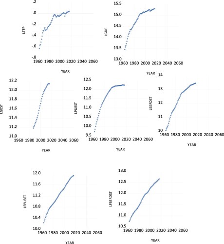
Figure 2. Effects of a permanent change of 0.005 (accumulated sum of the impulse responses) on public R&D stock in the VECM until 2050. The first graph indicates the type and size of the shock. The left axes measure differences to baseline at the lower curve. The right-hand axes measure levels of the shock scenario, baseline, and actuals at the higher set of curves. Confidence intervals are for policy scenarios. Their shift is roughly the same as that from baseline and therefore the lines are on each other.

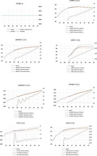
Figure 3. Effects of a permanent intercept change of 0.005 (accumulated sum of the impulse responses) on GBARD stock in the VECM until 2050. Other information as in Figure 2.

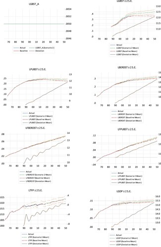
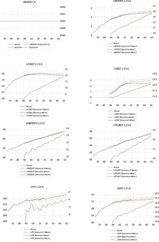
Figure 4. Effects of a permanent shock of 0.005 (accumulated sum of the impulse responses) on private R&D stock in the VECM until 2050. Other information as in Figure 2.

4. Methodology

4.1 The VECM approach

We are looking at simultaneous equation relations for the links GDP-TFP, TFP-priv R&D, priv-public R&D and others for foreign R&D variables as explained above. For the empirical models, the choice of methods always depend on how many variables and interactions are held to be essential. Deleidi and Mazzucato (2021) use four variables in the SVAR; in VECMs, Soete, Verspagen, and Ziesemer (2022) use five or six variables, and this papers uses seven. The advantage of the VECM method used here is that for all variables one can analyze the two-way causalities in estimation and simulations. It is reported below that variables have unit roots or near unit roots. The adequate methodological choice for a simultaneous equation model with unit roots is a VECM with a test on the number of cointegrating equations, as structural VARs serve other purposes (see Kilian and Lütkepohl 2017). This choice has several other advantages. What is of interest are the long-term relations, which correspond to the theory outlined in the literature section and should have statistical significance. The VECM approach generates a difference equation system in the seven variables mentioned above. We assume from the beginning and show later that they are all endogenous. Simulations allow for supplementing the regression results with effects including feedback from all variables and long-run disequilibrium.

We write a VAR underlying the VECM below in levels as follows: (1) $y=A_{1}y\left(-1\right)+A_{2}y\left(-2\right)+Cx+u$(1) Here y is the (7, 1)-vector (7 rows, 1 column) of the K = 7 variables. All variables are dependent on the lags of all others.¹² In the presence of unit roots, defined as levels of variables dependent on their own of lags with coefficients summing to unity, and cointegration, defined as a linear combination of variables that is stationary, a VECM approach is appropriate. In particular, r cointegrating equations, each abbreviated as CE, provide information on long-term relations in addition to a VAR model in differences. The VECM, which can be derived through rearrangement of the underlying VAR of equation (1(1) $y=A_{1}y\left(-1\right)+A_{2}y\left(-2\right)+Cx+u$(1) ) (see appendix based on Greene 2003, 1004), is written as follows. (2) $dy=\alpha {\text{β}}^{\mathrm{\prime }}y\left(-1\right)+Bdy\left(-1\right)+Fx+u$(2) If the term αβ’y(−1) were absent, we would basically have a system for the seven variables in differences regressed on the lags of all seven differenced variables with one lag less than for the levels in (1). Such estimation in differences avoids problems from variables with unit roots. A_p and B, for (1) and (2) respectively, is the (7, 7) matrix of coefficients of the (7, 1)-vector of lagged terms with lag p = 1,2, and perhaps more or less, as obtained from testing for lag length. C and F are a (7, 2)-matrices of the coefficients of the vector of exogenous variables x’ = (c, t), in the first instance only constant and time trend; in the application we also add unity dummies for the periods before the data revisions. β is a (9,r)-matrix of coefficients of the long-term relations, where cointegration tests provide the number r and it includes a constant and a coefficient for a time trend enhancing the number of variables in the long-term relations to 9, some of which must have zero coefficients.¹³ CE = β’y(−1) = E(u(−1)) = 0 represents the long-term relations; α is the (7, r)-matrix of adjustment coefficients indicating how strongly the left-hand side of the model reacts to dis-equilibrium, u(−1) ≠ 0. The econometric analysis of cointegrated variables leads to several possible outcomes. If the result from cointegration tests is r = 0, no cointegrating relation, equation (2(2) $dy=\alpha {\text{β}}^{\mathrm{\prime }}y\left(-1\right)+Bdy\left(-1\right)+Fx+u$(2) ) should be estimated without the term αβ’y(−1). If 0 < r < K, equation (2(2) $dy=\alpha {\text{β}}^{\mathrm{\prime }}y\left(-1\right)+Bdy\left(-1\right)+Fx+u$(2) ) is estimated as written. If r = K there are no unit eigenvalues in the system, and the model should be estimated in levels as in equation (1(1) $y=A_{1}y\left(-1\right)+A_{2}y\left(-2\right)+Cx+u$(1) ) irrespective of the uni-variate unit root tests (see Patterson 2000; Davidson and MacKinnon 2004; Kilian and Lütkepohl 2017). If all adjustment coefficients in α for one of the seven equations turn out to be insignificant, the dependent variable of that equation is called weakly exogenous because it does not react to disequilibrium deviations from the long-term relations.¹⁴ A crucial property to be tested for is that the VECM is stable, implying that the long-term relations return to their equilibrium value. Otherwise, the model is invalid for statistical reasons (Lütkepohl 2005; Pesaran 2015). The practical difficulty is to find the number r of long-term relations. We use the Johansen tests consisting of the trace test and the maximum-eigenvalue test. Hjalmarsson and Österholm (2010) suggest rejecting a null hypothesis of having at most r cointegrating equations, and by implication at least K-r unit roots (unit eigenvalues), in the presence of near unit roots only if both tests reject it. This leads to a conservatively low number of cointegrating relations. This is different from the suggestion of Jusélius, Framroze Møller, and Tarp (2014) to be aware of the low power of unit root tests in case of I(1) variables and be conservative against the hypothesis of having a unit root in the system; one would choose a low number of unit roots, K-r, and therefore a high number of cointegrating equations, r. In order to clarify whether a higher or lower number of cointegrating equations should be used, Kilian and Lütkepohl (2017) suggest testing of pairwise, triple wise etc. cointegrated relations. For example, if one test result is r = K – 1, we have K-1 pairwise cointegrated relationships; if the alternative is r = K-2, we have r triple wise relationships. If we can find r cointegrated pairs of variables, which are economically meaningful and statistically significant, the result r = K-1 is the preferred number of cointegrated equations, because, for example, two pairs give more information than one triple of variables.¹⁵ The estimation method is maximum likelihood. Having obtained the long-term relations, they can be renormalized (considering footnote 13) in order to make sure that the cointegrating equations are economically meaningful and the coefficients are statistically significant. From an estimated version of (2), the long-run growth rates for y in natural logarithms, with equilibrium in the long-term relations, β’y(−1) = 0, and year dummies phased out as in the figures below, can in principle be calculated as dy = c(I-B)⁻¹.¹⁶

Finally, if variables were I(2), the differenced terms in (2) would be I(1) and in case of cointegration β’y(−1) may also be I(1) but can also be I(0). Then we would have three I(1) expressions in (2). If they are cointegrating, (2) could still be used (see equation (16.5) in Jusélius (2006)); if not, the I(2) model may be useful.

In the second step, we will carry out shock analyses by way of increasing the intercept of the equation(s) for the growth rates of domestic public R&D, GBARD, private R&D and foreign private and public R&D by 0.005, a half percentage point, and comparing the baseline and the new solution.¹⁷ Permanent intercept changes are equivalent to the ‘accumulated sum of the impulse responses … where the same shock occurs in every period from the first’ (EViews 12 2020) unless the generalized impulses of Pesaran and Shin (1998) are used, which also take contemporaneous correlation of the residuals of the equations into account. The increase of the intercept makes sure that the variable of its equation changes first and all others only later (see Figures 2–4).¹⁸ A shock of a half percent may be small enough to leave the model unaffected and the policy not being subject to the Lucas critique (see Kilian and Lütkepohl 2017).¹⁹ This can show whether or not additional R&D of these variables generates positive or negative effects for complements or substitutes among the other R&D variables, TFP and GDP, and allows calculating the rates of return, as well as seeing whether Japan obtains positive knowledge spillovers or predominantly negative competition effects.

4.2 Net gains and internal rates of return

The additional benefit from permanent changes of all variables for each year is the achieved difference of the GDP from baseline to the extent that they stem from changes in TFP. The additional costs are 0.005 of the R&D shock variable in the initial year, and later the yearly additional private and public investment. The method of using shocks in a dynamic model results in exact numbers of yearly changes in real time. Subtracting the yearly costs from the yearly benefits yields the yearly gains. Discounting them at a conventional rate of 4% or any other rate allows adding them up and seeing whether they are positive. In addition, when the costs precede the benefits one can calculate the internal rate of return (irr), which is defined as the discount rate that brings the sum of discounted present values (DPV) to zero. This latter method may be problematic though for cases where gains go from negative to positive and then to negative and to positive again because it can have several rates of return as solutions.²⁰

5. Estimation results for the VEC model applied to the case of Japan

5.1 Estimation results²¹

All variables have a unit root with probability 0.2 or higher. Only two of the coefficients of the lagged dependent variable in the ADF equation are higher than 0.95, suggesting that the other variables have only near unit roots.²² Differenced variables are stationary if we use the F-statistic as the lag length criterium for the test of LGBST. We do not have to deal with I(2) variables.

Results for uni-variate unit roots suggest testing for the cointegration rank r and the number of unit roots, (7-r), in the system using the maximum-eigenvalue and trace tests for VECMs. The summary of the results for the standard procedure to get the VECM is as follows (see Appendix VECM basics). For the underlying VAR model, the optimal lag length is two. The VAR model is unstable though for one or two lags. However, the vector-error correction model with one lag presented below is stable in growth rates. Kilian and Lütkepohl (2017) suggest testing of pairwise cointegrated relations, which leads to r = 6. In Table A.1 of ‘Appendix VECM basics’ we show the test results for pairwise cointegrating equations. The estimated long-term relations (3)-(8) going into the VECM (9)-(15) are as follows.²³ (3) $CE1=E\left(u_1\left(-1\right)\right)=0=LFBERDST\left(-1\right)\text{–}0.175LGBST\left(-1\right)-0.0265t\text{–}9.13$(3) $\left[-13.24\left]\right[-35.0\right]$ (4) $CE2=E\left(u_2\left(-1\right)\right)=0=LTFP\left(-1\right)-0.248LFBERDST\left(-1\right)+3.056$(4) $\left[-20.7\right]$ (5) $CE3=E\left(u_3\left(-1\right)\right)=0=LTFP\left(-1\right)\text{–}0.05LBERDST\left(-1\right)-0.006t+0.911$(5) $\left[-10.2\left]\right[-15.9\right]$ (6) $CE4=E\left(u_4\left(-1\right)\right)=0=LGDP\left(-1\right)\text{–}0.475LBERDST\left(-1\right)+0.00167t-9.02$(6) $\left[-57.35\left]\right[3.15\right]$ (7) $CE5=E\left(u_5\left(-1\right)\right)=0=LFPUBST\left(-1\right)-0.643GDP\left(-1\right)-0.0173t-1.111$(7) $\left[-48.6\left]\right[-25.9\right]$ (8) $CE6=E\left(u_6\left(-1\right)\right)=0=LFPUBST\left(-1\right)-0.41LPUBST\left(-1\right)-0.0226t-5.67$(8) $\left[-22.5\left]\right[-46.94\right]$

The long-term relations should be economically meaningful and statistically significant. They may have two way causality. For example, GDP provides the means for private R&D and private R&D is often said to drive growth. We normalize one coefficient in each long-term relation to unity in a way that keeps regression coefficients small, because in the presence of unit roots coefficients are under suspicion of going to zero with low t-values if there is no proper cointegration; these small coefficients should not be set to unity (Boswijk 1996). The cointegrating equations show important results, with t-values in brackets. Mission R&D, LGBST, is often internationally coordinated and therefore related to foreign private R&D, LFBERDST, in CE1. Foreign private R&D stimulates domestic TFP according to CE2 and, perhaps, vice versa. Foreign private R&D can be a spillover effect suggesting a positive sign or a threat of competition, suggesting a negative sign unless stimulation dominates (Luintel and Khan 2004). The sign in CE2 suggests that spillovers or stimulating competition are dominating in Japan in the long run. Domestic TFP is generated by domestic private R&D in CE3. Domestic private R&D is larger when GDP is higher, after detrending, in CE4. Foreign public R&D, LFPUBST, is a response to Japanese growth, LGDP, in CE5.²⁴ Domestic public R&D, LPUBST, is closely related to foreign public R&D because public research is internationally connected. Combining equations (6)-(8) indicates that there is a positive long-term relation between private and public R&D for Japan after elimination of the other variables. All variables are de-trended by the time trend t (see Wooldridge 2013, chapter 10.5) except for equation (4(4) $CE2=E\left(u_2\left(-1\right)\right)=0=LTFP\left(-1\right)-0.248LFBERDST\left(-1\right)+3.056$(4) ) where the coefficient is close to zero and highly insignificant; dropping it leads only to minimal changes in the estimated coefficients. Exogenous time trends in the long-term relations and constants in the equations for the growth rates make sure that all variables grow in the stable steady state. However, six long-term relations can determine only six variables and therefore the whole system determines ultimately all the variables for each point in time. Ultimately, the path of all variables depends on the solution of the whole system. The long-term results are only partial effects. We need the whole model to get the effects of permanent policy changes.

When estimating the vector-error correction model we set adjustment coefficients with t << 1 to zero. When going to stricter values, the p-value for the chi-square test on all restrictions decreases strongly; this may be legitimate, but the model then goes away from ‘letting the data speak’. The t-values for adjustment coefficients shown in equation (9)–(15) below suggest that we are not very restrictive in setting coefficients to zero. The model is stable in growth rates also after imposing the constraints.

The complete model, including the long-term relations CE1, … , 6 from equations (3) to (8), is as follows (with first-difference terms and dummies in an appendix). The estimation period is 1989-2016, reduced by two periods because of the lags. We use as abbreviation Y for LGDP, A for LTFP, B for LBERDST, P for LPUBST, G for LGBST, a ‘*’ for the corresponding foreign variables and D for the first difference with respect to time (t-values in parentheses for adjustment coefficients and intercepts). Equations (9)-(15) (plus the differenced terms in the appendix) are the estimated version of the corresponding vector-equation system (2) in the methodology section. The terms CE1 – CE6 in (9) to (15) are abbreviations equal to those in (3)-(8), corresponding to β’y(−1) in (2), but allowing for dis-equilibrium. In other words, insertion of CE1-CE6 from (3)–(8), corresponding to β’y(−1) in (2), into (9)-(15) would give the whole estimated model corresponding to (2) above in the VECM methodology. (9) $D\left(G\right)=0.666CE1+1.666CE2-1.81CE3+0.586CE4+0.533CE5\text{–}0.186CE6+0.02$(9) $\left[3.3\right]\left[2.04\right]\left[-1.866\right]\left[1.38\right]\left[2.66\right]\left[-1.07\right]\left[0.75\right]$ (10) $D\left(B\ast \right)=-0.333CE1-0.44CE4-0.4CE5+0.0046$(10) $\left[-4.78\right]\left[-2.9\right]\left[-4.77\right]\left[0.17\right]$ (11) $D\left(A\right)=1.127CE1\text{–}1.4CE4+1.23CE5-1.39CE6+0.069$(11) $\left[3.0\right]\left[-1.6\right]\left[2.2\right]\left[-5.17\right]\left[0.48\right]$ (12) $D\left(B\right)=-4.6CE2+3.8CE3+0.0775$(12) $\left[-4.62\right]\left[3.79\right]\left[1.21\right]$ (13) $D\left(Y\right)=0.998CE1+1.676CE3-2.82CE4+1.45CE5-2.04CE6+0.12$(13) $\left[2.268\right]\left[6.8\right]\left[-2.81\right]\left[2.23\right]\left[-5.966\right]\left[0.73\right]$ (14) $D\left(P\ast \right)=-2.126CE2+1.9CE3-0.3CE4-0.383CE5+0.127CE6+0.04$(14) $\left[-7.33\right]\left[6.3\right]\left[-2.14\right]\left[-5.12\right]\left[2.53\right]\left[3.78\right]$ (15) $D\left(P\right)=-0.189CE1+0.828CE2-0.619CE3+0.0617CE4+0.956CE5+1.04CE6-0.013$(15) $\left[-0.85\right]\left[1.29\right]\left[-0.82\right]\left[-1.48\right]\left[-4.5\right]\left[6.98\right]\left[-0.39\right]$

As all equations have cointegrating equations on the right-hand side, all variables are strictly endogenous. Adj. R-squared for equations (9)-(15) are 0.97, 0.90, 0.326, 0.91, 0.38, 0.97, 0.96. The lowest t-values for slopes are for the first and the third term in equation (15(15) $D\left(P\right)=-0.189CE1+0.828CE2-0.619CE3+0.0617CE4+0.956CE5+1.04CE6-0.013$(15) ). The coefficients are not small though and putting the adjustment coefficient to zero causes a large drop in the value of p = 0.949 of the chi-square statistic testing the over-identifying constraints.

The data in Figure 1 show that TFP growth has constant growth rates before 1973, from 1974 to 1990, and later, with lower rates in each later period. Hayashi and Prescott (2002) and Kaihatsu and Kurozumi (2014) interpret the trend in TFP (not corrected for human capital) as exogenous and see it as responsible for the slow growth. However, TFP is endogenous in our VECM as adjustment coefficients are statistically significant in equation (11(11) $D\left(A\right)=1.127CE1\text{–}1.4CE4+1.23CE5-1.39CE6+0.069$(11) ). For the period of stagnation, Bottazzi and Peri (2007) point out that R&D employment is stagnant in Japan. Branstetter and Nakamura (2003) point out that private R&D expenditure flows have stagnated or grown slowly during the 1990s leading to mostly decreasing growth rates of private (and public) R&D stocks in our data and simulations below. This goes together in our data with decreasing growth rates of domestic private and public R&D stocks in Figure 1.

5.2 Baseline simulation results and permanent changes of gbard, public and private R&D in the VECM

The results described so far only indicate regression coefficients but do not include indirect effects of all variables influencing each other mutually. In particular, variables that have no direct impact can have indirect impacts via other variables. Figures 2–4 include the baseline simulation of VECM (9)-(15) considering all interactions from 1000 stochastic runs. To see the reaction to permanent changes, we impose a permanent change of 0.005 on the constant of the public investment equation (15(15) $D\left(P\right)=-0.189CE1+0.828CE2-0.619CE3+0.0617CE4+0.956CE5+1.04CE6-0.013$(15) ) for (DLPUBST) in scenario 1 and on the constant of equation (9(9) $D\left(G\right)=0.666CE1+1.666CE2-1.81CE3+0.586CE4+0.533CE5\text{–}0.186CE6+0.02$(9) ) for GBARD stock for (DLGBST) in scenario 2. The hypothetical structural policy change is captured by shifts of the intercept. Structural change, short-term and long-terms effects work together through the whole system of difference equations and are shown in the Figures 2–4 after each shock.²⁵

Figure 2 shows that – after the shock on public investment indicated by the starting value above zero in the upper left graph – the public R&D stock keeps growing beyond its baseline value. Private R&D, LBERDST, shows a similar pattern both going about 6 percent beyond baseline. GBARD increases slightly more, going 8 percent beyond baseline. TFP increases much less, about 0.4 percent, and GDP up to 3 percent, half as much as BERD stock and PUBST, indicating that R&D/GDP ratios increase when R&D stock growth increases in this scenario. Foreign private R&D goes up, as does foreign public R&D; Japan creates positive spillovers or incentives for strategic reactions for foreign private and public R&D for the model of this period. As Bernstein and Mohnen (1998) find no spillovers from Japan to the USA (for an earlier period though) and Luintel and Khan (2004) even negative ones, it is likely that Japan generates spillovers to or stimulates R&D expenditures of the EU. This is in line with positive effects found by Luintel and Khan (2004) on other countries than the USA. But here it comes explicitly from public R&D shocks, which is in line with the finding of Luintel and Khan (2004) that business R&D has weaker effects than total R&D. The effects are only slightly positive for TFP (with the exception of one year) but higher for GDP, meaning that R&D has other dynamic effects than just those via TFP, which may be wage increases through additional labour demand from higher R&D expenditures, as well as more employment of labour and capital inflows (reduced outflows) as higher TFP increases their marginal product.

Figure 3 shows that after a permanent change of the intercept of the equation for GBARD, indicated by the positive value in the upper-left graph, GBARD (LGBST) goes up relative to baseline. Public and private R&D stocks are above baseline after increasing GBARD in Japan. TFP is also above baseline but much less than the private and public R&D. The overall effect on GDP is positive, more than for TFP but less than for R&D. Japan’s shock to GBARD increases foreign private and public R&D and again less so than domestic R&D variables in terms of percentages.

Figure 4 shows that a permanent intercept change of 0.005 on private R&D has a positive effect on public R&D and on GBARD. TFP and GDP react also slightly positively. Also, foreign R&D variables react positively, again less than domestic R&D variables but more than TFP.

Table 2 presents the average values of the differences for scenario and baseline for the years 1989–2050 for the plots of Figures 2–4 all evaluated at expected values. All effects are positive. The highest effect on TFP comes from a shock on private R&D. But effects from GBARD changes are about equally strong. Effects on GDP are stronger than for TFP. This indicates that not only money goes into additional hiring, but rather additional labour and capital are demanded for production because of higher marginal products and perhaps wages are increased.²⁶ Foreign private and public R&D react positively to all three permanent policy changes just discussed. The values may seem small at first sight. However, for the sake of comparison: German entrepreneurs urged their government to participate in TTIP because of estimated gains of 10 billion Euros when the German GDP was about Euro3300 billion; this implies a percentage value of 0.003 of GDP to be compared with the last column of Table 2, where all three values are larger than that for TTIP.

Table 2. Effects from shocks on public R&D, GBARD, and private R&D: Percentage difference from baseline averaged from 1989 to 2050.

	Effects →From shock ↓ (a)	Domestic mission R&D, GBARD	Domestic Public R&D	Domestic private R&D	For. public R&D	For. private R&D	TFP	GDP
VECM	public R&D	0.0443	0.0385	0.0372	0.009	.0094	.0044	.0218
	GBARD	0.1825	0.106	0.1443	.0445	.0341	.0127	.0702
	Private R&D	0.11	0.0958	0.1346	.0399	.0283	.0137	.0689

(a) Shock size is 0.005 on the intercept of growth rate equations (9), (12), and (15).

If effects are positive, they may still not justify the costs in terms of public and private R&D, or conversely, if effects are small, they may be beneficial if increases on costs are low relative to the effects on GDP. In particular, the effects so far were measured in percentages whereas the R&D stock variables and GDP are of different size. This suggests comparing benefits and costs in terms of comparable values. Table 3 presents the years of positive gains, the results from calculating the gains (difference of shocks to baseline of GDP, minus change of cost flows for private and public R&D, including GBARD) as share of GDP, their sum of present values discounted at 4%, and internal rates of return.

Table 3. Net gains, DPV, and internal rates of return (IRR) to additional public R&D, GBARD, and private R&D.

Model	Shock	Years of gains; average gain/GDP (a)	Sum DPV (4%) in bill. $	Internal rate of return (%) (payback period) (b)	Initial costs
VECM	public R&D	1990–2050; 0.00286	126.366	234.6 (2)	0.5% of public R&D stock
	GBARD	1990–2050; 0.007	460.849	205.6 (2)	0.5% of GBARD stock
	private R&D	1990–2050; 0.00864	651.554	305.5 (2)	0.5% of private R&D stock

(a) Only the yearly percentage share of TFP change multiplied to the GDP is counted as benefit.

(b) Payback period is the number of years that it takes to have a positive sum of gains after discounting at the internal rate of return. Period 1 is the shock period 1989.

The first row shows results for the permanent change of public R&D compared to baseline, the second row for the shock on GBARD compared to baseline, and the third row for the shock on private R&D. These are financial results comparing the policy shocks relative to baseline. The scenarios in Table 3 have long-lasting gains until the horizon of 2050.²⁷ GBARD shocks have initial costs 0.005GBST in 1989, where GBST is roughly half of PUBST; later costs are captured as those of publicly and privately performed R&D. The gains per year are larger for the private than the public shocks in the VECM, and GBARD ranks in between. The sum of present values discounted at 4% interest over all years has the same ranking. The internal rate of return is also higher for private than for public R&D shocks; for shocks on GBARD they are slightly lower than for public and private R&D, but still as high as 200%. The rates of return are higher than the marginal products of total R&D in the literature on static models and in the same order of magnitude of the social rate of return as in Ogawa, Sterken, and Tokutsu (2016) and in the middle of the range found by Luintel and Khan (2004, 908) going from negative to 453%. The reason for the high rates is that the traditional approach turns elasticities into a marginal product in an a-temporal way or as a steady-state solution of an error correction model. In our approach of calculating net gains per year and discounting them with the internal rate of return, it also plays a role whether the gains come about early or late. The higher internal rates of return for private R&D suggest that the gains are obtained early as indicated by the short payback period in Table 3. Short but early periods of gains lead to high internal rates, and late gains interrupted by phases of losses would lead to low returns. Comparing Figures 1–3, Japan’s increase of the ratio of GBARD flows over GERD-BERD in Table 1 from 0.5 to unity seemingly is ensuing through a slowdown of GBARD and public R&D²⁸ both growing less quickly than GDP, whereas private R&D continues growing faster than GDP.

There are a couple of reasons why the rates of return are so high and payback periods so short. First, we do not consider the additional costs for capital and labour in production of the higher GDP, because it is exactly the purpose of growth policies to increase employment and wages and attract international capital. We do not include these indirect effects in the costs, which are not only costs for firms but also income for households, and therefore cancel out from a welfare perspective. Second, the analysis is ex-post, whereas decisions are taken under uncertainty and risk; implicit risk premia may be high here although the state takes a lot of the risk burdens. Third, a log–log specification as used here has decreasing marginal products in case of positive coefficients; by implication, rates of return may be higher if less has been done in terms of inputs. Fourth, most policies affect international R&D positively, which generates spillover repercussions and competitive reactions to the economy under consideration, which may reinforce the domestic effects, especially if R&D reaction functions under oligopolistic conditions are upward sloping with or without spillovers (see Ziesemer 2022).

Table 2 and Figures 2–4 indicate that foreign private and public R&D stocks are endogenous for Japan, whereas Luintel and Khan (2004) find only a 9% probability for this when foreign R&D stocks are built from the sum of private and public foreign flows rather than having two foreign stocks, for private and public R&D separately. Defining foreign public and private R&D stocks separately and using the method of shock reactions makes the impact of Japan’s innovation on foreign R&D visible as being positive in our paper. Although they react only slightly differently from each other in Figures 2–4 but considering the disaggregation contributes to finding an impact of Japan on both foreign R&D stocks.

6. The impact of Japan’s public R&D on European private R&D in two pooled mean group (PMG) estimator models

In this section we show explicitly that Japan’s public R&D has a positive impact on private R&D of European countries. Castellacci and Natera (2013) suggest doing this type of analysis in the framework of a panel VECM with pooled data. However, their approach implies slope homogeneity. The authors mitigate the problem by way of sub-dividing their panel of 87 countries into five separate panels at different income levels with on average about 17 countries, for which then slope homogeneity is assumed. However, Ziesemer (2021c) has shown the limits to a common model for R&D variables with slope homogeneity for seven European countries. Moreover, the approach of using country groups comes at the cost of another potential problem called cross-unit cointegration (Gonzalo and Granger 1995): The variables of all groups may be cointegrated with the variables of the countries in the richest group doing most of the R&D (ignoring the less likely possibility of cointegration with lower income groups). In such a case, the results may be wrong if the neglected relation with richer countries has an impact on the results Soete, Verspagen, and Ziesemer (2020, 2022)., Ziesemer (2021c, 2022) and this paper in its earlier sections mitigate the problem of cross-unit cointegration by way of using variables for foreign private and public R&D. Most probably, approaches to cross-unit cointegration will always remain somewhat imperfect, because for a panel of N countries with each K variables there are actually K times N variables whereas the VECM approach can handle not more than 10 variables (Pesaran 2015).²⁹ In this section, we also use variables for foreign private and public R&D to mitigate the cross-unit-cointegration problem and we apply the suggestion of Castellacci and Natera (2013) in a slightly modified way using the PMG (pooled mean group) maximum likelihood estimator to mitigate the slope homogeneity assumption. The PMG is a single-equation error-correction model for each country in a panel with the restriction that the slopes in the long-term relation are the same for all countries. Therefore, the PMG has slope homogeneity still in the long-term relation but not in the short-term coefficients and the adjustment coefficients multiplied to the long-term relation, for which we obtain and report only the panel-average values and their p-values. ‘Under some regularity assumptions the parameter estimates of this model are consistent and asymptotically normal for both stationary and non-stationary I(1) regressors' (Asteriou and Hall 2021).³⁰ As we have data only for a low number of countries, which is a disadvantage when averaging over the heterogenous parameters, we analyze one panel of seven European countries (BEL, FRA, DEU, DNK, GBR, ITA, NLD) as in Ziesemer (2021c) and a slightly larger panel of 14 European countries (the previous seven and AUT, ESP, FIN, IRL, NOR, PRT, SWE). The data are described in Tables A.2 and A.3. We use the information from the earlier sections of this paper and the VECMs for seven countries in Ziesemer (2021c) to specify the long-term relations for the two panels. However, for the current research question, mission-oriented R&D is not important and therefore we can drop it. Comparing the results for the two samples will show how strong the heterogeneity is. Data are made in the same way as indicated for Japan above. We replace TFP from PWT through labour-augmenting technical change (LATC) from Ziesemer (2021d) because TFP in PWT is set to unity for the base period for all countries, which takes out the cross-country differences in TFP for the base year. LATC is derived from a CES production function under alternative assumptions on the elasticity of substitution. For the samples used here the log of LAT from a CES function with elasticity of substitution 0.8, denoted LTH08 works best.³¹ Equation numbers ending with ‘a’ are for the sample with seven countries and equation numbers ending with ‘b’ are for the sample with 14 countries. ‘ … ’ indicates that unreported current and lagged differences of the regressors and lagged dependent variables follow. An Appendix provides econometric details of the estimates. P-values in parentheses are abbreviated as (0.00) if all four digits are zero. (16a) $D\left(LGDP\right)=-0.0475(LGDP-0.98LTH08+0.014t)\dots$(16a) $\left(0.0136\right)\left(0.00\right)\left(0.00\right)$ (16b) $D\left(LGDP\right)=-0.04(LGDP-1.16LTH08+0.01t)\dots$(16b) $\left(0.0001\right)\left(0.00\right)\left(0.00\right)$

For both samples a larger LTH level leads to a larger GDP level with an elasticity close to unity. The time trend mimics omitted variables like capital and labour and captures detrending of the variables. (17a) $D\left(LTH08\right)=-0.0164(LTH08-0.073LBERDST\text{–}1.01LFPUBST+0.0234t)\dots$(17a) $\left(0.0135\right)\left(0.011\right)\left(0.00\right)\left(0.00\right)$ (17b) $D\left(LTH08\right)=-0.091(LTH08-0.148LBERDST)\dots$(17b) $\left(0.0013\right)\left(0.00\right)$Foreign public R&D is significant in the technical change equation for five of seven countries in the VECMs of Ziesemer (2021c) as it is here for the small sample but not for the larger sample, where panel heterogeneity is probably too strong to allow for statistical significance. (18a) $D\left(LBERDST\right)=-0.0576\left(LBERDST-0.242LPUBST-0.457LPUBSTJPN+1.93LFPUBST-0.069t\right)\dots$(18a) $\left(0.00\right)\left(0.0055\right)\left(0.00\right)\left(0.00\right)\left(0.00\right)$ (18b) $D\left(LBERDST\right)=-0.04\left(LBERDST-0.8LPUBST-0.27LPUBSTJPN+2.549LFPUBST-0.079t\right)\dots$(18b) $\left(0.004\right)\left(0.00\right)\left(0.00\right)\left(0.00\right)\left(0.00\right)$In both samples, European private R&D is driven by domestic and Japanese public R&D as suggested in the literature review, but foreign public R&D reduces domestic private R&D in general, indicating that Japan’s position is an exception. The signs do not change when one of the public R&D variables is taken out. It would require another paper to explore whether there are more countries’ whose public R&D is an exception. The trend term indicates that private R&D is growing more quickly than the combination of European, Japanese, and foreign public R&D as in the data of Archibugi and Filippetti (2018); as the trend coefficient is very high, we probably have some collinearity here among all variables. Equations (18a, b) support the results of Sveikauskas (2007), Rehman, Hysa, and Mao (2020), and Soete, Verspagen, and Ziesemer (2022) regarding the effect of public on private R&D, and adds the effects of Japanese and other foreign R&D. (19a) $D\left(LPUBST\right)=-0.043\left(LPUBST-0.85LBERDST+0.0022t\right)\dots$(19a) $\left(0.0857\right)\left(0.0000\right)\left(0.056\right)$ (19b) $D\left(LPUBST\right)=-0.03\left(LPUBST-0.926LBERDST+0.0039t\right)\dots$(19b) $\left(0.0466\right)\left(0.000\right)\left(0.0002\right)$Public R&D responds positively to domestic private R&D. The time trend indicates that public R&D grows on average more quickly than private R&D.³² Equations (18a,b) and (19a,b) together show that there is two-way causality between private and public R&D, and both are endogenous. Then, putting them together into other equations is likely to lead to collinearity. Therefore, treating them pairwise or triple wise as in VEC or PMG models is preferable. (20a) $D\left(LFPUBST\right)=-0.033(LFPUBST-0.294LFBERDST-0.182LTH08-0.0146t)\dots$(20a) $\left(0.0009\right)\left(0.0001\right)\left(0.00\right)\left(0.00\right)$ (20b) $D\left(LFPUBST\right)=-0.05(LFPUBST-0.493LFBERDST-0.376LTH08-0.01t)\dots$(20b) $\left(0.00\right)\left(0.00\right)\left(0.075\right)\left(0.00\right)$Foreign public R&D goes together with foreign private R&D, which is analogous to the domestic variable in (19a,b). In addition, foreign public R&D responds to European countries’ level of technical change. (21a) $D\left(LFBERDST\right)=-0.0055\left(LFBERDST-0.888LGDP\right)\dots$(21a) $\left(0.00\right)\left(0.0024\right)$ (21b) $D\left(LFBERDST\right)=-0.00995\left(LFBERDST-1.085LGDP\right)\dots$(21b) $\left(0.00\right)\left(0.00\right)$Foreign private R&D reacts to European GDP. Using TFP or foreign public R&D or a combination also yields good results but a slightly lower log-likelihood. The only way to get a higher likelihood is to include all variables but mission-oriented R&D. However, this would mean putting together several cointegrated relations on the right-hand side of one equation leading often to unexpected signs because of collinearity.

The adjustment coefficients in equations (16a,b) – (21a,b) are between −0.005 and −0.095. These are highly significant and therefore panel long-term or cointegrating relations exist (see Pesaran, Shin, and Smith 1999). The implied near unit roots are 1 minus these values. These are small deviations from a unit root implying slow adjustments stretched out over many years. From these results and the fact that each variable also appears in one of the other equations as second variable we can conclude that the second variable in each equation also has a near unit roots.

The major purpose of this section was to show that Japan’s public R&D has a positive externality to European private R&D in (18a,b) as concluded from earlier parts of this paper in connection with a discussion of the literature. In order to reveal is importance, we also show that the externality enhanced private European R&D increases European productivity according to equation (17a,b), and productivity enhances GDP according to equations (16a,b). Foreign private R&D reacts to this increase of GDP in (21a,b) and stimulates foreign public R&D in (20a,b), which in turn dampens the initial effect on domestic private R&D in (18a,b) and enhances technical change in (17a). Having carried out all regressions for two country panels reveals some heterogeneity in the coefficients but also that we are close to finding a common model for the relation between R&D variables, productivity and GDP for European countries.

7. Discussion

We have shown that flows of GBARD relative to public R&D have gone from 0.5 to unity over time for Japan using data for 1988–2016. We have made GBARD stock data and used them in a VEC model. Public R&D data show the strongest slowdown of all variables. GBARD stocks have a long-term relation with foreign private R&D in Japan. Shocks to GBARD have positive effects for the period 1990–2050 on all other variables in the VECM for Japan; this is a major new result from this paper. Mission-oriented R&D stimulates all variables positively in the short run except for foreign public R&D, which is affected negatively. In the long run, mission-oriented R&D stimulates foreign private R&D because mission-oriented R&D often is integrated in international programs, or, alternatively, stimulates competition leading to a chain reaction in terms of long-run relations: foreign BERD stimulates TFP, which triggers domestic private R&D; together TFP and domestic private R&D stimulate GDP; foreign public R&D reacts to Japan’s additional growth, to which Japan responds with its own public R&D. This way, a permanent change of mission-oriented R&D stimulates all other variables. This compares to only two papers dealing with mission-oriented R&D. Deleidi and Mazzucato (2021) have used US data for the period 1947–2018 for military mission R&D flow data showing a positive effect from expenditure shocks for eight years. Ziesemer (2021c) has used data for the period 1970–2014 for seven EU countries for mission-oriented R&D stocks built from five GBARD items and finds positive effects until the horizon 2040 from shocks setting in during the early 1970s. Three of the seven internal rates of return in that paper are higher than the one for Japan in this paper and four are lower. The long-term relations (3)-(8) can be compared to those of seven European countries in Ziesemer (2021c, Table 1) showing the ‘heterogeneity limits to a common model’.

Moreover, our VECM analysis has shown that a public R&D shock affects GBARD, business R&D, TFP, GDP and foreign private and public R&D positively, in the short and the long run, and they are all endogenous. Additional private R&D in the form of a permanent change has even slightly better effects than public R&D and GBARD. Thus, it is hard to sustain that Japanese R&D has no effects on other countries’ R&D decisions. Another important result is that GBARD reacts to all variables changed by shocks; it is clearly endogenous although it is a policy variable. Foreign private R&D is cointegrated with TFP, which therefore is endogenous, as all other variables in the model are.

The net gains from shocks on the three domestic R&D stock variables (GBARD, private and public R&D) are strongly positive with high internal rates of return.

Moreover, shocks to foreign private R&D have positive effects on Japanese private and public R&D, TFP, GDP, and on GBARD, whereas shocks to foreign public R&D have negative effects (see working paper version). The common belief that foreign R&D capital stocks have stimulated Japan’s R&D (Luintel and Khan 2004) is supported here for the long-term effect of foreign public R&D stocks with a positive effect on domestic public R&D in CE6 and for foreign private R&D on TFP and GBST in CE1 and CE2. Splitting foreign R&D into private and public generates interesting results, which are different in their effects. Given the result of Bernstein and Mohnen (1998) of no spillovers from Japan to the USA, and our result that Japan’s public R&D stimulates foreign R&D, additional public R&D of Japan should stimulate public and/or private R&D in the EU. We show this explicitly for pooled mean-group estimators of the major relations between R&D variables, TFP and GDP for two small panels of European OECD countries.

8. Conclusion

Our recommendation as to ‘what policy changes would allow productivity to grow again’ (Hayashi and Prescott 2002) has two logical steps. As long as the causes for low TFP growth discussed in the literature continue to exist, we suggest a special form of an R&D policy. First, all three forms of R&D have very high rates of return and therefore they should all be enlarged. Expanding them together seems to a good policy. Second, analyses that are more detailed than our macroeconomic study should identify needs for missions and their adjustments and compare them to other suggestions, both of which are beyond the scope of this paper, also because of the special role of Japanese expenditure for defense and defense-related R&D links the economic questions to those of foreign policy. Third, Fukao, Makino, and Settsu (2021) show that growth rates of human capital and TFP have fallen to 0.31% and 0.28% respectively. This is fairly low compared to the panel average of 0.8–1.1% for 69 countries considered in Ziesemer (2021d). However, for a leading country this may be harder to increase than for the average. Policy should try to improve upon the lack of human capital growth according to the literature on Japanese growth discussed in Ziesemer (2020), which emphasizes the need for more PhD level education and IT personnel.

However, the search for causes of the low productivity growth and policies to deal with it goes on. Ikeuchi et al. (2022) emphasize the exit of high productivity firms, which may be the mirror image of support for weak industries considered in Ziesemer (2020) or a lack of comparative advantage. Hosono and Takizawa (2022) investigate the ‘contribution’ of bubble and crisis periods. Okamuro and Sakuma (2021) investigate the relation between tax-policy rules and private R&D. Our results hopefully show that the analysis of public and mission-oriented R&D is closely linked and should be considered as well. Given the specific nature of mission-oriented R&D it may be useful to link it to sector-specific work on Japan’s productivity (Betts 2021). Finally, Japan’s public R&D may have a positive impact on European R&D and may stimulate global growth through this effect.

Acknowledgement

I gratefully acknowledge useful comments from four anonymous referees, Hugo Hollanders, Georg Licht, Luc Soete, Bart Verspagen, and participants of two meetings at EU DG R&I. Special thanks go to Bart Verspagen for providing data from the UNU-MERIT database.

Disclosure statement

No potential conflict of interest was reported by the author(s).

Notes

1 The official expression is Government budget appropriations or outlays for RD. The traditional abbreviation GBAORD was changed recently to GBARD.

2 Ergas (1987) emphasizes aerospace, electronics, and nuclear energy as the largest in terms of government R&D funding. OECD data called GBARD (and thereby the statistical concepts) are available for several countries since the end of the 1960s.

3 In some parts of the literature, the VECM is called ‘cointegrated VAR’. See Jusélius (2006).

4 If marginal productivity conditions hold with inequality, adding complementary slackness as usual generates equality and goes into estimated constants.

5 It is discussing defence, environment, health, space, and energy.

6 Chiang (1991) attributes the first use of ‘mission-oriented’ to Ergas (1987). The paper also discusses several problems for slow diffusion of defense R&D.

7 For reasons of length, analysis of shocks to foreign private and public R&D are shown only in the working paper of 2022.

8 Already in Ergas (1987), Table 3, less than 50% of government financed R&D is performed in the government sector in five countries.

9 Data sets for Australia, Switzerland, Greece, Island, and New Zealand are incomplete.

10 More recent GBARD flow data are characterized as ‘different definition, preliminary, estimated, forecast’ in OECD-MSTI.

11 In contrast, OECD measures of TFP do include human capital as only labour and capital are subtracted from GDP. As R&D also includes human capital, a regression of both including a third human capital variable as found in some articles is likely to be strong because of the common human capital data included and may lead to multi-collinearity.

12 Unlike other areas, we do not assume that there is another model with contemporaneous regressors behind it. We assume that the effect from a change in each variable to the others takes at least a year.

13 The expression αβ’ in (2) is not unique. It can be written as αβ’ = αQ^-1Qβ’ for any invertible matrix Q, with I = Q^-1Q and Q as (r,r) matrices. To make β’ unique, we have to impose rxr constraints determining Q (Pesaran 2015). The so-called Johansen default writes Qβ’ = (I_r,r, β_K-r) meaning that the first part is the identity matrix with r times 1 on the diagonal and zeros otherwise, and β_K-r is a matrix with K-r elements in its r columns; with K=7 and r=6 in our case below, we have one row of freely estimated coefficients below the identity matrix. Division of any of the equations β’y(-1) = 0 (renormalization) does not changes the solution but it changes the standard deviations and t-values of the coefficients. If an equation is divided by β_i, the coefficient of variable i becomes unity and can be connected to economic intuition or theory. We do not assume that there is an underlying structural model, because the long-term relations of a VECM typically capture theoretical relations. In Jusélius (2006) these are the basic relations from monetary macroeconomics. In Ziesemer (2021a) the first-order marginal productivity conditions of the theoretical model are linked to some of the long-term relations in Soete, Verspagen, and Ziesemer (2022).

14 Other definitions of exogeneity deal with having, in addition, no impact on a variable y from other variables in the differenced part because of zero elements in B of equation (2(2) $dy=\alpha {\text{β}}^{\mathrm{\prime }}y\left(-1\right)+Bdy\left(-1\right)+Fx+u$(2) ) (Patterson 2000). Then we would have an additional exogenous variable x with coefficient matrix F extended, and this reduces the number of endogenous variables by one. The differenced equation then does not depend on any other variable and is a purely autoregressive process of the variable in differenced form confirming that it has a unit root.

15 Of course, it would be desirable to have more data points than just 30. However, there are quite a few papers, which give very plausible results with this low number of observations. What is more important in the presence of non-stationary variables is that pairwise cointegrated equations are not overloaded with additional variables. Van Elk et al. (2015, 2019) show that it is much harder to get plausible results when all R&D variables are used in only one TFP equation.

16 This is of course independent of the assumption of an underlying structural model.

17 See Lau (1997), equation (22(19a) $D\left(LPUBST\right)=-0.043\left(LPUBST-0.85LBERDST+0.0022t\right)\dots$(19a) ), for a formalization of permanent changes in VARs and VECMs related to exogenous and endogenous growth theory.

18 (Non-linear) ARDL models also can be used to obtain long-term error-correction terms. But they are single-equation methods, which cannot capture the feedback effects among the variables of a system of endogenous variables when shocks go through a system of equations either reinforcing or weakening the partial effects as captured by the regression coefficients. The literature related to this paper has no indications of asymmetric non-linear effects.

19 Such simulations are policy scenarios and should not be mis-interpreted as forecasting the absence of any structural change until 2050. Moreover, if the growth model of Ziesemer (2021a) is used as underlying theory, the estimated parameters in the long-term relations would be deep parameters in Lucas’ terminology.

20 This method using the exact time resolution from a VECM for the rate of return calculation, has first been developed and used by Soete, Verspagen, and Ziesemer (2020).

21 A more detailed explanation regarding unit roots and cointegration is given in the working paper version from 2022.

22 By convention, near unit roots have coefficients between 0.8-0.95, and unit roots have coefficients between 0.95 and unity or even slightly higher (Enders 2015; Patterson 2000).

23 In the vein of checking for deviation between this paper and Ziesemer (2020) we have developed this normalization, which makes the two papers as similar as possible in regard to shock effects from public and private R&D, in spite of the introduction of GBARD, LGBST. See also footnote 24 for a further comparison of the papers. A working paper version from 2019 shows negative effects of GBARD shocks; it may have end-of-sample bias through the financial crisis 2007–2013 because there the sample period ends in 2014. With end-of-sample crises the revenues of R&D expenditures are likely to come a bit later. The negative returns with end of sample in 2014 in the working paper from 2019 and highly positive one with end of sample in 2017 in this paper indicates a delay of two or three years.

24 The sign for LGDP is different in Ziesemer (2020). Reasons may be that (i) the period is much more recent here, indicating some structural change over time; (ii) the eigenvectors of the data matrix for seven variables here instead of six in Ziesemer (2020) may differ; (iii) the VECM here has one lag whereas Ziesemer (2020) has three lags because of more data; (iv) the 2008 dummy is significant here but was not in Ziesemer (2020). Shock results go into the same direction in both papers. Rates of return for private R&D are higher and for public R&D lower than in Ziesemer (2020).

25 We do not have enough data to test for structural breaks in the estimation.

26 See David and Hall (2000) for the related theory, and Goolsbee (1998) and Wolff and Reinthaler (2008) for some evidence.

27 Therefore, assumptions on stopping or continuing policies when they generate losses do not matter.

28 Archibugi and Filippetti (2018) document the relative fall of public R&D relative to private R&D.

29 As in economic theory and VECM estimation or any other regression approach the success depends on choosing the most important variables for each research question. Otherwise, the later detection of important control variables may overthrow earlier results.

30 See Asteriou and Hall (2021) for an introduction to the PMG. ‘The homogeneity test results suggest that further efforts are needed also to take account of within group heterogeneity.’ (Pesaran 2015, 745). The Hausman test for slope homogeneity indicated in Asteriou and Hall (2021) is only valid for N>T. We cannot offer more than statistical significance of the slope in the long-term relation. As the method holds for I(0) and I(1) variables Pesaran, Shin, and Smith (1999) do not test separately for panel unit roots or panel cointegration; the estimates imply results for this, which we discuss in due course.

31 This should not be overrated because under some panel heterogeneity in different samples other CES values may work better.

32 We could add foreign private and mission-oriented R&D in the smaller sample or replace private R&D by mission-oriented R&D in the larger sample, but then the log-likelihood would be reduced in both cases, and adjustment coefficients get statistically insignificant for the smaller sample.

Appendices

1. VECM basics

Each VECM has an underlying VAR from which it is derived. If the VAR has lag p, taking differences, the first step to get the VECM, leads to having one lag less. From Greene (2003), p. 1004 “Consider the VAR representation of the model ${\mathrm{y}}_{\mathrm{t}}=\mathrm{\Gamma }{\mathrm{y}}_{\mathrm{t}\text{-}1}+{ϵ}_{\mathrm{t}},$where the vector yt is [yt, zt ]. Now take first differences to obtain ${\mathrm{y}}_{\mathrm{t}}-{\mathrm{y}}_{\mathrm{t}\text{-}1}=(\mathrm{\Gamma }-\mathrm{I}){\mathrm{y}}_{\mathrm{t}\text{-}1}+{ϵ}_{\mathrm{t}}$or $\mathrm{\Delta }{\mathrm{y}}_{\mathrm{t}}=\pi {\mathrm{y}}_{\mathrm{t}\text{-}1}+{ϵ}_{\mathrm{t}}.$

The VAR has lag 1 in levels; the VECM has lag 0 in differences, one less than the VAR in levels.

The following computer output documents that the optimal lag length of the VAR underlying our VECM is p = 2. LGBST data go only until 2016.

Table

VAR Lag Order Selection Criteria
Endogenous variables: LGBST LFBERDST LTFP LBERDST LGDP LFPUBST LPUBST
Exogenous variables: C DUM13 DUM08 DUM96 @TREND
Date: 10/17/22 Time: 15:30
Sample: 1967 2017
Included observations: 28
Lag	LogL	LR	FPE	AIC	SC	HQ
0	614.6611	NA	2.53e−27	−41.40436	−39.73911	−40.89528
1	935.9476	367.1846	1.33e−35	−60.85340	−56.85679	−59.63159
2	1072.709	87.91798*	1.32e−37*	−67.12206*	−60.79409*	−65.18754*

* indicates lag order selected by the criterion.

LR: sequential modified LR test statistic (each test at 5% level).

FPE: Final prediction error.

AIC: Akaike information criterion.

SC: Schwarz information criterion.

HQ: Hannan-Quinn information criterion.

The following computer output shows that the VECM is stable in growth rates

Table

Roots of characteristic polynomial
Endogenous variables: LGBST LFBERDST
LTFP LBERDST LGDP LFPUBST
LPUBST
Exogenous variables: DUM13 DUM08
DUM96
Lag specification: 1 1
Root	Modulus
1.000000	1.000000
0.732771 − 0.630810i	0.966889
0.732771 + 0.630810i	0.966889
0.864734 − 0.225022i	0.893533
0.864734 + 0.225022i	0.893533
0.698117 − 0.526690i	0.874512
0.698117 + 0.526690i	0.874512
−0.417884 − 0.601178i	0.732149
−0.417884 + 0.601178i	0.732149
0.130543 − 0.685732i	0.698047
0.130543 + 0.685732i	0.698047
0.242660 − 0.475397i	0.533747
0.242660 + 0.475397i	0.533747
−0.451747	0.451747

VEC specification imposes 1 unit root(s).

TABLE A.1 OVER HERE

Appendix first differences of the estimated VECM Model

Abbreviations: LBERDST, LFBERDST, LPUBST, LFPUBST, LGDP, LTFP, LGBST are the natural logs of domestic and foreign private and public R&D stocks, gross domestic product, total factor productivity, and GBARD.

VECM properties

Sample (adjusted): 1989 2016. Included observations: 28 after adjustments. t-statistics in [ ]. Convergence achieved after 260 iterations. Restrictions identify all cointegrating vectors. LR test for binding restrictions (rank = 6): Chi-square(12): 5.241231. Probability: 0.949432.

D(LGBST) D(LFBERDST) D(LTFP) D(LBERDST) D(LGDP) D(LFPUBST) D(LPUBST)

Table

D(LGBST(−1))	0.456	0.066	0.346	0.246	0.280	−0.006	0.548
	[ 4.08]	[ 0.596]	[ 0.572]	[ 0.918]	[ 0.395]	[−0.128]	[ 3.989]
D(LFBERDST−1)	0.181	0.315	−1.191	−0.962	−1.510	−0.240	0.414
	[ 0.694]	[ 1.224]	[−0.846]	[−1.536]	[−0.913]	[−2.28353]	[ 1.288]
D(LTFP(−1))	0.661	0.278	−1.551	−0.248	−2.093	−0.039	0.441
	[ 1.964]	[ 0.833]	[−0.851]	[−0.306]	[−0.978]	[−0.288]	[ 1.059]
D(LBERDST(−1))	−0.009	0.315	1.235	1.264	0.944	0.187	−0.312
	[−0.034]	[ 1.168]	[ 0.836]	[ 1.925]	[ 0.544]	[ 1.696]	[−0.926]
D(LGDP(−1))	−0.599	−0.082	2.106	0.674	2.660	0.148	−0.455
	[−1.707]	[−0.237]	[ 1.109]	[ 0.798]	[ 1.193]	[ 1.047]	[−1.050]
D(LFPUBST(−1))	−0.237	−0.508	−5.707	−3.647	−7.032	−0.492	0.259
	[−0.302]	[−0.656]	[−1.348]	[−1.938]	[−1.414]	[−1.55604]	[ 0.267]
D(LPUBST(−1))	0.140	0.243	−0.104	0.256	−0.409	−0.022	0.476
	[ 0.987]	[ 1.730]	[−0.135]	[ 0.751]	[−0.454]	[−0.386]	[ 2.722]
C	0.020	0.005	0.069	0.078	0.123	0.041	−0.013
	[ 0.752]	[ 0.174]	[ 0.483]	[ 1.216]	[ 0.733]	[ 3.789]	[−0.394]
DUM13	0.008	0.008	0.023	0.016	0.031	0.002	−0.016
	[ 1.768]	[ 1.773]	[ 0.937]	[ 1.433]	[ 1.068]	[ 0.979]	[−2.838]
DUM08	0.000	0.005	0.050	0.014	0.063	−0.003	0.012
	[ 0.002]	[ 1.440]	[ 2.449]	[ 1.481]	[ 2.627]	[−1.867]	[ 2.656]
DUM96	−0.017	0.002	−0.021	−0.013	−0.026	−0.001	0.012
	[−3.528]	[ 0.319]	[−0.836]	[−1.139]	[−0.866]	[−0.728]	[ 1.988]

Table

R-squared	0.989	0.959	0.725	0.965	0.748	0.989	0.985
Adj. R-squared	0.973	0.900	0.326	0.914	0.383	0.974	0.964
Sum sq. resids	0.000	0.000	0.002	0.000	0.003	0.000	0.000
S.E. equation	0.003	0.003	0.014	0.006	0.016	0.001	0.003
F-statistic	61.23	16.23	1.81	18.97	2.05	63.13	45.87
Log likelihood	140.6	140.9	93.3	116.0	88.8	165.9	134.7
Akaike AIC	−8.826	−8.847	−5.449	−7.070	−5.127	−10.638	−8.404
Schwarz SC	−8.017	−8.038	−4.640	−6.261	−4.319	−9.829	−7.595
Mean dependent	0.033	0.029	0.003	0.036	0.012	0.027	0.014
S.D. dependent	0.015	0.008	0.017	0.021	0.021	0.006	0.017
Determinant resid covariance (dof adj.)	1.38E−39
Determinant resid covariance	1.99E−42
Log likelihood	1064.400
Akaike information criterion	−64.10003
Schwarz criterion	−56.15438
Number of coefficients	167

Econometric details of PMG estimations

TABLE A.2 OVER HERE

TABLE A.3 OVER HERE

Table

Equation	Sample	Obs.	No. of models evaluated	ARDL type of selected model(a)	s.e. of regression	Log likelihood
16a	1965–2016	364	25	2, 2, 2	0.01	1159.8
16b	1965–2016	728	25	2, 2, 2; max 5	0.0198	2233.5
17a	1969–2016	351	25	2, 3,3,3; max 5	0.0187	938.37
17b	1968–2016	707	25	3, 2, 2; max 5	0.0276	1689.47
18a	1969–2016	351	25	3,1,1,1,1; max5(3)	0.0068	1303.29
18b	1969–2016	692	25	3,1,1,1,1; max5(3)	0.0097	2375.01
19a	1970–2016	344	25	4,4,4; max 5	0.0067	1276.65
19b	1969–2016	688	16	3,1,1,1; max 4	0.0086	2398.47
20a	1966–2016	357	9	2,3.3.3; max 3	0.002273	1699
20b	1967–2016	700	25	3,4,4,4;	0.002	3417.94
21a	1966–2016	357	16	3,3	0.0032	1565.37
21b	1967–2016	700	16	3,4	0.0031	3089.75

Maximum dependent lags is 4 (Automatic selection) unless indicated otherwise; model selection method is Akaike info criterion (AIC).

The notation ARDL (x,y,z) indicates the number of lagged differenced terms used in the regression including lag zero¹

1 The presentation in Asteriou and Hall (2021) differs in that there are only lagged differences.

and including and starting with the dependent variable. For example, ARDL (1,3,3) means that the dependent variable appears only on the left-hand side and of the two dynamic regressors three variables of each regressor are included outside the long-term relation. If a trend is included, the differenced term is unity and the third or higher lags are redundant because it equals the second lags, which is also dt=1 and therefore is dropped but included in the count. Allowing for more (less) lags we get a larger (lower) number of models to be evaluated, but a lower (higher) number of observations. We bias the choice for the maximum number of lags intentionally in favour of getting similar results for both sample.

Table A.1. Pairwise Johansen cointegration tests, p-values.

Test (a)	Trace test	Trace test	Max-eigenvalue	Max-eigenvalue
Hypothesis	No coint. equation	At most 1	No coint. equat.	At most 1
LGBST,LFBERDST(c)	0.0004	0.2584	0.0003	0.2584
LFBERSTD, LTFP (b)	0.1037	0.4996	0.0919	0.4996
LTFP, LBERDST	0.1427	0.3910	0.1743	0.3910
LBERDST, LGDP	0.0012	0.3685	0.0007	0.3685
LGDP, LFPUBST (d)	0.0111	0.0482	0.0736	0.0482
LFPUBST,LPUBST(c)	0.0070	0.1568	0.0151	0.1568

(a) Based on VECM 1967–2017 with one lag.

(b) Based on VECM 1967–2017 with two lags.

(c) Adding dummies dum08, dum13, and dum96 would lead to two cointegrating equations for these pairs of variables or absence of unit eigenvalues. Relating the variables in terms of levels requires only statistical significance.

(d) The low p-values suggest that there is no unit eigenvalue in this system of two variables and only statistical significance for this pair of variable is required.

Table A.2. Data description of small sample of 7 European countries 1963–2017.

	LGDP	LOG(TH08)	LBERDST	LPUBST	LFPUBST	LFBERDST	LPUBSTJPN
Mean	13.42076	1.843367	10.51738	10.12548	12.89156	13.48943	11.62050
Median	13.67750	1.931421	10.57019	10.37690	12.92300	13.58173	11.91396
Maximum	14.97432	2.213102	12.80206	12.02957	13.70296	14.41835	12.23792
Minimum	11.19053	0.965248	6.744390	7.314201	11.69796	12.26703	9.712675
Std. Dev.	0.999543	0.286769	1.246342	1.099550	0.492707	0.576561	0.700289
Skewness	−0.420496	−0.924725	−0.491604	−0.424441	−0.233651	−0.239929	−1.099822
Kurtosis	1.921422	3.077434	2.886665	2.162118	2.056274	1.854314	3.073846
Jarque-Bera	29.53984	54.10956	15.46858	22.46597	17.51282	24.36435	76.49303
Probability	0.000000	0.000000	0.000438	0.000013	0.000157	0.000005	0.000000
Sum	5086.469	698.6359	3986.086	3837.556	4885.903	5112.494	4404.168
Sum Sq. Dev.	377.6548	31.08534	587.1734	457.0056	91.76351	125.6558	185.3731
Observations	379	379	379	379	379	379	379

Table A.3. Data description of sample of 14 European countries 1963–2017.

	LGDP	LOG(TH08)	LBERDST	LPUBST	LFPUBST	LFBERDST	LPUBSTJPN
Mean	12.72269	1.821388	9.571315	9.329586	12.90327	13.49881	11.59295
Median	12.47103	1.856213	9.713017	9.300465	12.94095	13.59097	11.91396
Maximum	14.97432	2.861371	12.80206	12.02957	13.74456	14.46309	12.23792
Minimum	9.977576	0.853379	4.658052	5.825222	11.69796	12.26703	9.712675
Std. Dev.	1.150286	0.326947	1.650398	1.341166	0.494917	0.581444	0.728243
Skewness	0.120921	−0.193389	−0.425938	−0.101956	−0.230863	−0.236550	−1.073502
Kurtosis	2.069678	3.329749	2.741167	2.276327	2.020811	1.830743	2.966287
Jarque-Bera	29.64454	8.288154	24.73841	17.52375	37.60172	51.04408	147.9287
Probability	0.000000	0.015858	0.000004	0.000157	0.000000	0.000000	0.000000
Sum	9796.470	1402.469	7168.915	6941.212	9935.519	10394.08	8926.568
Sum Sq. Dev.	1017.509	82.20191	2037.411	1336.454	188.3608	259.9815	407.8295
Observations	770	770	749	744	770	770	770

References

- Archibugi, Daniele, and Andrea Filippetti. 2018. “The Retreat of Public Research and its Adverse Consequences on Innovation.” Technological Forecasting & Social Change 127: 97–111. doi:10.1016/j.techfore.2017.05.022.
- Asteriou, D., and S. G. Hall. 2021. Applied Econometrics. Fourth Edition. Hampshire: Palgrave Macmillan.
- Baumol, W. J. 1967. “Macroeconomics of Unbalanced Growth: The Anatomy of Urban Crisis.” The American Economic Review 57 (3): 415–426.
- Becker, B. 2015. “Public R&D Policies and Private R&D Investment: A Survey of the Empirical Evidence.” Journal of Economic Surveys 29 (5): 917–942. doi:10.1111/joes.12074.
- Bernstein, J. I., and P. Mohnen. 1998. “International R&D Spillovers Between U.S. and Japanese R&D Intensive Sectors.” Journal of International Economics 44: 315–338.
- Betts, Caroline. 2021. Accounting for Japan’s Lost Score. MPRA Paper No. 109285. 21 August.
- Boeing, P., and P. Hünermund. 2020. “A Global Decline in Research Productivity? Evidence from China and Germany.” Economics Letters 197: 1–4. doi:10.1016/j.econlet.2020.109646.
- Boswijk, H. P. 1996. “Testing Identifiability of Cointegrating Vectors.” Journal of Business & Economic Statistics 14 (2): 153–160. doi:10.1080/07350015.1996.10524641.
- Bottazzi, L., and G. Peri. 2007. “The International Dynamics of R&D and Innovation in the Long Run and in the Short Run.” The Economic Journal 117: 486–511. doi:10.1111/j.1468-0297.2007.02027.x.
- Branstetter, L., and Y. Nakamura. 2003. Structural impediments to growth in Japan, NBER Conference Report series. Chicago and London: University of Chicago Press, 191–223.
- Castellacci, Fulvio, and Jose Miguel Natera. 2013. “The Dynamics of National Innovation Systems: A Panel Cointegration Analysis of the Coevolution Between Innovative Capability and Absorptive Capacity.” Research Policy 42 (3): 579–594. doi:10.1016/j.respol.2012.10.006.
- Chiang, J.-T. 1991. “From ‘Mission-Oriented’ to ‘Diffusion-Oriented’ Paradigm: The new Trend of U.” S. Industrial Technology Policy. Technovation 11 (6): 339–356. Also available online as MIT Sloan School of Management WP 3225-90-BPS, Nov 1990.
- David, P. A., and B. H. Hall. 2000. “Heart of Darkness: Modeling Public–Private Funding Interactions Inside the R&D Black box.” Research Policy 29: 1165–1183.
- Davidson, R., and J. G. MacKinnon. 2004. Econometric Theory and Methods. New York: Oxford University Press.
- Deleidi, Matteo, and Mariana Mazzucato. 2021. “Directed Innovation Policies and the Supermultiplier: An Empirical Assessment of Mission-Oriented Policies in the US Economy.” Research Policy 50 (2): 1–13. doi:10.1016/j.respol.2020.104151.
- Eaton, J., and S. Kortum. 1997. “Engines of Growth: Domestic and Foreign Sources of Innovation.” Japan and the World Economy 9: 235–259.
- Enders, W. 2015. Applied Econometric Time Series. 4th edition. City: Wiley.
- Ergas, Henry. 1987. “Does Technology Policy Matter?” In Technology and Global Industry: Companies and Nations in the World Economy, edited by Bruce R. Guile, and Harvey Brooks, 191–245. Washington, D.C.: National Academy Press.
- ESIR. 2017. Towards a Mission-Oriented Research and Innovation Policy in the European Union. An ESIR Memorandum (December 2017). Brussel: European Commission.
- EViews 12. 2020. User’s Guide II. Seal Beach: IHS Global.
- Feenstra, R. C., R. Inklaar, and M. P. Timmer. 2015. “The Next Generation of the Penn World Table.” American Economic Review 105 (10): 3150–3182. doi:10.1257/aer.20130954.
- Foray, D., D. C. Mowery, and R. R. Nelson. 2012. “Public R&D and Social Challenges: What Lessons from Mission R&D Programs?” Research Policy 41: 1697–1702. doi:10.1016/j.respol.2012.07.011.
- Fukao, K., T. Makino, and T. Settsu. 2021. “Human Capital and Economic Growth in Japan: 1885–2015.” Journal of Economic Surveys 35 (3): 710–740. doi:10.1111/joes.12419.
- Gonzalo, J., and C. Granger. 1995. “Estimation of Common Long-Memory Components in Cointegrated Systems.” Journal of Business & Economic Statistics 13 (1): 27–35.
- Goolsbee, A. 1998. Does government R&D policy mainly benefit scientists and engineers? NBER WP 6532.
- Greene, W. H. 2003. Econometric Analysis. India: Pearson Education.
- Hall, B., J. Mairesse, and P. Mohnen. 2010. “Measuring the Returns to R&D.” In Handbook of the Economics of Innovation, Vol. 2, edited by Bronwyn H. Hall, and Nathan Rosenberg, 1033–1082. Amsterdam: North-Holland.
- Hayashi, F., and E. C. Prescott. 2002. “The 1990s in Japan: A Lost Decade.” Review of Economic Dynamics 5: 206–235. doi:10.1006/redy.2001.0149.
- Hjalmarsson, E., and P. Österholm. 2010. “Testing for Cointegration Using the Johansen Methodology When Variables are Near-Integrated: Size Distortions and Partial Remedies.” Empirical Economics 39: 51–76. doi:10.1007/s00181-009-0294-6.
- Hosono, Kaoru, and Miho Takizawa. 2022. “Japan's Productivity Stagnation: Using Dynamic Hsieh–Klenow Decomposition.” Contemporary Economic Policy 40: 218–232. doi:10.1111/coep.12547.
- Ikeuchi, Kenta, Young Gak Kim, Hyeog Ug Kwon, and Kyoji Fukao. 2022. “Productivity Dynamics in Japan and the Negative Exit Effect.” Contemporary Economic Policy 40: 204–217. doi:10.1111/coep.12546.
- Jusélius, K. 2006. The Cointegrated VAR Model: Methodology and Applications. Oxford: Oxford University Press.
- Jusélius, K., N. Framroze Møller, and F. Tarp. 2014. “The Long-Run Impact of Foreign Aid in 36 African Countries: Insights from Multivariate Time Series Analysis.” Oxford Bulletin of Economics and Statistics 76 (2): 153–184. doi:10.1111/obes.12012.
- Kaihatsu, S., and T. Kurozumi. 2014. “What Caused Japan’s Great Stagnation in the 1990s?” Evidence from an Estimated DSGE Model. Journal of the Japanese and the International Economies 34: 217–235. doi:10.1016/j.jjie.2014.08.002.
- Kaldor, N., and J. A. Mirrlees. 1962. “A Growth Model with Induced Technical Progress.” Review of Economic Studies 29: 174–190.
- Khan, M., and K. B. Luintel. 2006. “Sources of Knowledge and Productivity: How Robust is the Relationship?” OECD STI Working Paper 2006/6.
- Kilian, L., and H. Lütkepohl. 2017. Structural Vector Autoregressive Analysis. Cambridge: Cambridge University Press.
- Lau, S.-H. P. 1997. “Using Stochastic Growth Models Unit Roots and Breaking Trends.” Journal of Economic Dynamics and Control 21: 1645–1667.
- Luintel, K. B., and M. Khan. 2004. “Are International R&D Spillovers Costly for the United States?” The Review of Economics and Statistics 86 (4): 896–910.
- Luintel, K. B., M. Khan, and K. Theodoridis. 2014. “On the Robustness of R&D.” Journal of Productivity Analysis 42: 137–155. doi:10.1007/s11123-013-0360-0.
- Lütkepohl, H. 2005. New Introduction to Multiple Time Series Analysis. Berlin: Springer Science & Business Media.
- Mazzucato, M. 2018. Mission-Oriented Innovation Policy: Challenges and Opportunities. In European Commission (2018) Science, Research, and Innovation Performance of the EU 2018. Strengthening the foundations for Europe's future. Brussels, 396–427. Download: https://ec.europa.eu/info/sites/info/files/rec-17-015-srip-report2018_mep-web-20180228.pdf.
- METI. 2018. Report on Digital Transformation (DX). Summary. Download 29-7-2021, 16:39 from https://www.meti.go.jp/english/press/2018/pdf/0907_004a.pdf.
- Moretti, Enrico, Claudia Steinwender, and John Van Reenen. 2020. The Intellectual Spoils of War? Defense R&D, Productivity and International Spillovers. NBER Working Paper No. 26483.
- Mukerji, Vatsala. 1963. “A Generalized S.M.A.C. Function with Constant Ratios of Elasticity of Substitution.” The Review of Economic Studies 30 (3): 233–236.
- OECD. 2017. The impact of r&d investment on economic performance: a review of the econometric evidence. DSTI/STP/NESTI(2017)12.
- Ogawa, K., E. Sterken, and I. Tokutsu. 2016. International R&D Spillovers and Marginal Social Returns on R&D. CESIFO WORKING PAPER NO. 6255.
- Okamuro, Hiroyuki, and Yohei Sakuma. 2021. The Effects of R&D Tax Incentive Reform on R&D Expenditures: The Case of 2009 Reform in Japan. TDB-CAREE Discussion Paper Series, No. E-2021-04, August.
- Pallante, Gianluca, Emanuele Russo, and Andrea Roventini. 2021. Does mission-oriented funding stimulate private R&D? Evidence from military R&D for US states, LEM Working Paper Series, No. 2020/32, Scuola Superiore Sant'Anna, Laboratory of Economics and Management (LEM), Pisa.
- Patterson, K. 2000. An Introduction to Applied Econometrics: A Time-Series Approach. New York: Palgrave Macmillan.
- Pesaran, M. H. 2015. Time Series and Panel Data Econometrics. Oxford: Oxford University Press.
- Pesaran, H. H., and Y. Shin. 1998. “Generalized Impulse Response Analysis in Linear Multivariate Models.” Economics Letters 58: 17–29.
- Pesaran, M. H., Y. Shin, and R. P. Smith. 1999. “Pooled Mean Group Estimation of Dynamic Heterogeneous Panels.” Journal of the American Statistical Association 94 (446): 621–634.
- Phelps, E. S. 1966. “Models of Technical Progress and the Golden Rule of Research.” The Review of Economic Studies 33 (2): 133–145.
- Rehman, Naqeeb Ur, Eglantina Hysa, and Xuxin Mao. 2020. “Does Public R&D Complement or Crowd-out Private R&D in pre and Post Economic Crisis of 2008?” Journal of Applied Economics 23 (1): 349–371. doi:10.1080/15140326.2020.1762341.
- RIETI. 2008. Innovation Process and Performance: Findings and lessons from inventors surveys in Japan, the U.S., and Europe. Download from 29-7-2021 from https://www.rieti.go.jp/en/events/08011101/summary3.html.
- Shell, Karl. 1967. “A Model of Inventive Activity and Capital Accumulation.” In Essays on the Theory of Optimal Economic Growth, edited by Karl Shell, 67–85. Cambridge, MA: The MIT Press.
- Soete, L., K. Guy, et al. 2009. The Role of Community Research Policy in the Knowledge-Based Economy. Brussel: EC Expert Group.
- Soete, L., B. Verspagen, and T. H. W. Ziesemer. 2020. “The Productivity Effect of Public R&D in the Netherlands.” Economics of Innovation and New Technology 29 (1): 31–47. doi:10.1080/10438599.2019.1580813.
- Soete, L., B. Verspagen, and T. H. W. Ziesemer. 2022. “The Economic Impact of Public R&D: An International Perspective.” Industrial and Corporate Change 31 (1): 1–18. doi:10.1093/icc/dtab066.
- Soete, L. en A. Arundel (red.). 1993. An Integrated Approach to European Innovation and Technology Diffusion Policy. SPRINT. Brussel: European Commission.
- Sveikauskas, Leo. 2007. R&D and Productivity Growth: A Review of the Literature. U.S. Bureau of Labor Statistics, Working Paper 408, September.
- Van Elk, R., B. ter Weel, K. van der Wiel, and B. Wouterse. 2019. “Estimating the Returns to Public R&D Investments: Evidence from Production Function Models.” De Economist 167 (1): 45–87. doi:10.1007/s10645-019-09331-3.
- Van Elk, R., B. Verspagen, B. Ter Weel, K. Van der Wiel, and B. Wouterse. 2015. A macroeconomic analysis of the returns to public R&D investments. UNU-MERIT.
- Verspagen, B. 1995. “R&D and Productivity: A Broad Cross-Section Cross-Country Look.” Journal of Productivity Analysis 6 (2): 117–135.
- Vogt, W. 1973. “Zur Langfristigen ökonomischen Entwicklung Eines Kapitalistischen Systems.” Leviathan 1 (2): 161–188.
- Wada, S. 2008. Realizing Japan as a “Nation Built on Scientific and Technological Creativity”. Download from https://www.rieti.go.jp/jp/events/08011101/pdf/6-4_E_Wada_Shuichi_PPT_t.pdf at 29-7-2021, 17:37.
- Wolff, G., and V. Reinthaler. 2008. “The Effectiveness of Subsidies Revisited: Accounting for Wage and Employment Effects in Business R&D.” Research Policy 37: 1403–1412. doi:10.1016/j.respol.2008.04.023.
- Wooldridge, J. M. 2013. Introductory Econometrics: A Modern Approach. Fifth Edition. Mason: Cencage Learning South Western.
- Ziesemer, T. 1990. “Public Factors and Democracy in Poverty Analysis.” Oxford Economic Papers 42 (1): 268–280.
- Ziesemer, T. 1995. “Endogenous Growth with Public Factors and Heterogeneous Human Capital Producers.” FinanzArchiv/Public Finance Analysis 52 (1): 1–20.
- Ziesemer, T. H. W. 2020. “Japan’s Productivity and GDP Growth: The Role of Private, Public and Foreign R&D 1967–2017.” Economies 8 (4): 1–25. doi:10.3390/economies8040077.
- Ziesemer, T. H. W. 2021a. “Semi-endogenous Growth Models with Domestic and Foreign Private and Public R&D Linked to VECMs.” Economics of Innovation and New Technology 30 (6): 621–642. doi:10.1080/10438599.2020.1760423.
- Ziesemer, T. H. W. 2021b. “The Effects of R&D Subsidies and Publicly Performed R&D on Business R&D: A Survey.” Hacienda Pública Española/Review of Public Economics, IEF 236 (1): 171–205. doi:10.7866/HPE-RPE.21.1.6.
- Ziesemer, T. H. W. 2021c. “The Impact of Mission-Oriented R&D on Domestic and Foreign Private and Public R&D, Total Factor Productivity and GDP.” Journal of Applied Economics 24 (1): 460–477. doi:10.1080/15140326.2021.1963395.
- Ziesemer, T. H. W. 2021d. “Labour-augmenting Technical Change Data for Alternative Elasticities of Substitution: Growth, Slowdown, and Distribution Dynamics.” Economics of Innovation and New Technology. Online. doi:10.1080/10438599.2021.1956316.
- Ziesemer, T. H. W. 2022. “Foreign R&D Spillovers to the USA and Strategic Reactions.” Applied Economics 54 (37): 4274–4291. doi:10.1080/00036846.2022.2030042.