The Finnish Version of the Affinity for Technology Interaction (ATI) Scale: Psychometric Properties and an Examination of Gender Differences

Abstract

The pervasiveness of technical systems in our lives calls for a broad understanding of the interaction between humans and technology. Affinity for technology interaction (ATI) scale measures the tendency of a person to actively engage or to avoid interaction with technological systems, including both software and physical devices. This research presents a psychometric analysis of a Finnish version of the ATI scale. The data consisted of 796 responses of students in a Finnish university. The data were analyzed utilizing factor analysis and both nonparametric and parametric item response theory. The Finnish version of the ATI scale proved to be essentially unidimensional, showing high reliability estimates, and forming a strong Mokken scale. Hierarchical multiple regression analysis showed that men had a slightly higher affinity for technology than women when controlling for age and field of study; however the effect size was small.

1. Introduction

Urban legend or not, the famous quote from the 1950s allegedly attributed to Thomas J. Watson, a long-time chairperson and the CEO of International Business Machines, claimed that there would be market potential for only five electronic computers (IBM, 2007). The future turned out to be different, and today we live amid ubiquitous technical systems. The pervasiveness of different technological systems stretches out to many fields of life, including work (e.g., van Laar et al., 2017), education (e.g., Kim, Merrill, Xu, & Sellnow, 2021), sports (e.g., Cranmer et al., 2021), health (e.g., Tajudeen et al., 2021), culture (e.g., Kim & Lee, 2022), virtual life (e.g., Taufik et al., 2021), and even afterlife (Beaunoyer & Guitton, 2021). Thus, technological development poses several challenges which call for multidisciplinary, international and global research efforts (Stephanidis et al., 2019).

Scholars have identified mixed effects relating to how information and communication technologies affect our lives (Ali et al., 2020). Many effects are reciprocal and mediated by personality traits and other individual differences. For example, individual differences can affect self-disclosure in social media (Chen et al., 2015), usability assessment (Kortum & Oswald, 2018), gaming (Caci et al., 2019), online learning (Alabdullatif & Velázquez-Iturbide, 2020), and online privacy literacy and behavior (Sindermann et al., 2021). Furthermore, meta-reviews have documented gender differences relating to attitudes towards technology (Cai et al., 2017; Whitley, 1997): in general, men tended to have slightly more favorable attitudes towards technology. Information technology can facilitate personality research especially from the idiographic point of view (Matthews et al., 2021; Montag & Elhai, 2019) and, as Matthews et al. (2021) point out, socio-technological change might give rise to the evolution of the contemporary trait models in the future society. Thus, it is important to have valid constructs and psychometric instruments to discern individual differences and understand underlying phenomena relating to interactions between humans and technology.

A general concept for depicting the relationship between humans and technology is the person’s affinity with technological systems and devices. Edison and Geissler (2003) consider affinity for technology as an attitude and a “positive affect towards technology (in general).” Franke et al. (2019) define affinity for technology interaction as a question of “whether users tend to actively approach interaction with technical systems or, rather, tend to avoid intensive interaction with new systems.” In terms of technology interaction, it can be viewed as a key personal resource, and as such, it is of great importance considering the interaction between the user and technology.

One promising scale to assess human and technology interaction is the affinity for technology interaction (ATI) scale¹ developed by Franke et al. (2019). The scale was initially developed in English and German, and it is currently available as translations also in Italian, Spanish, Romanian, Persian, and Dutch. However, to our knowledge, besides the original English and German versions, no published analyses of the psychometric properties of the scale exist for other languages. In terms of cross-cultural research, confirmation of translations of scales plays a crucial role, especially when the scales are constructed to measure some universal constructs or phenomena (Cha et al., 2007).

This research presents a psychometric analysis of the Finnish version of the ATI scale. We elaborate on the subject by examining the gender differences relating to ATI. In other words, we address the validity evidence concerning the scale’s internal structure and it’s ability to capture differences and similarities (AERA, APA, & NCME, 2014). We use a comprehensive analytical process utilizing methodological triangulation and multiple sources of information. By presenting a psychometric analysis of the Finnish version of the scale, we aim to provide added value to the original research-based model of using ATI scale in measuring individual differences in affinity for technology interaction.

2. Materials and methods

2.1. Affinity for technology interaction (ATI) scale (Franke et al., 2019)

The starting point of the definition of ATI mentioned earlier is a realization that affinity for technology interaction and need for cognition (NFC) are closely related; following Schmettow and Drees (2014), Franke et al. (2019) propose that the two “should be conceptualized in a close relationship”. Relying on, for example, Cacioppo and Petty (1982), Cacioppo et al. (1996) and Fleischhauer et al. (2010), they note that NFC can be seen today as “the inter-individually varying, stable intrinsic motivation to engage in cognitively challenging tasks”. Given that NFC can be applied in different psychological domains, they see developing ATI in line with the construct of NFC as useful.

The purpose of Franke et al. (2019) was both to develop and validate a new scale to be able to assess ATI. Their goal was to provide “a highly economical and reliable unidimensional scale that is suitable for differentiating between users across the whole range of the ATI trait,” keeping in mind the focus that ATI has as a general interaction style in relation to technology (Franke et al., 2019). As a result, their ATI scale is a unidimensional 9-item scale having 3 reverse-worded (RW) items. All items are measured using a 6-point Likert scale. The shorter version of the scale (ATI-S) consisting of a subset of 4 items is currently available in German and in English (Wessel et al., 2019).

Franke et al. (2019) summarized the results of their validation process of ATI scale using multiple studies (N > 1500) as follows: first of all, the factor analyses indicated unidimensionality of the ATI scale. Secondly, their analysis revealed that reliability estimated using coefficient α ranged between good and excellent. Thirdly, when it comes to the need for cognition, geekism, technology enthusiasm, computer anxiety, control beliefs in dealing with technology, success in technical problem-solving and technical system learning, technical system usage, and the personality dimensions linked to Big Five, the expected relationships were supported by construct validity analysis. Fourth, when considering the ability of the ATI scale to differentiate between higher- and lower-ATI participants, item analysis and descriptive statistics showed that this was possible. Fifth, when taking into account analyses of demographic variables, the gender effect turned out to be large, the age effect small, and the educational background had no effect at all. Thus, the results showed that it could be possible to “discriminate between participants based on their differing tendency to actively engage in intensive (i.e., cognitively demanding) technology interaction” (Franke et al., 2019). The ATI scale has been used in varied contexts. These include studies on partially automated vehicles (e.g., Boelhouwer et al., 2020; Schartmüller et al., 2019), automated decision-making in health care (Schlicker et al., 2021), use of information technology among primary care physician trainees (Wensing et al., 2019), privacy concerns in users’ acceptance of e-Health technologies (Schomakers et al., 2019) and activity tracker usage (e.g., Attig & Franke, 2019), as well as augmented reality (Kammler et al., 2019).

2.2. Translation protocol

The translation of the original scale to Finnish was conducted as a forward-backward translation utilizing a committee approach (Brislin et al., 1973, pp. 46–47). The translation process, in general, followed the protocol proposed by Sousa and Rojjanasrirat (2011), excluding the pilot testing (Table 1). Two independent professional translators conducted the forward translations from the original English version of the scale. The first and second authors constructed the initial Finnish version based on the two professional translations. While the translations were conducted using the original English version of the scale, we also used the original German version of the ATI scale for creating the Finnish translation. A native German speaker and a German language teacher evaluated the connotations of a few essential wordings between the initial Finnish version and the original German version of the scale to achieve consistency between both original versions. After a few minor refinements, the initial translated version was back-translated to English by two independent professional translators. The back-translated versions proved excellent similarity with the original English version of the scale. The exact word–by–word equivalences of the back-translated versions compared to the original scale version were 70% and 76%, and when considering synonyms 77% and 85% respectively. Thus, the final translated Finnish version (Table 1) was chosen to be used in the primary data collection. The translations of the introductory text and Likert categories are presented in the Appendix A.

Table 1. The Finnish translation of the ATI scale.

Item	Finnish translation
ATI1	Perehdyn mielelläni teknisiin järjestelmiin yksityiskohtaisesti.
ATI2	Pidän uusien teknisten järjestelmien toimintojen kokeilemisesta.
ATI3	Olen tekemisissä teknisten järjestelmien kanssa lähinnä siksi, koska minun täytyy.
ATI4	Kun kohtaan uuden teknisen järjestelmän, kokeilen sitä innokkaasti ja perusteellisesti.
ATI5	Käytän mielelläni aikaa uuteen tekniseen järjestelmään tutustumiseen.
ATI6	Minulle riittää, että tekninen järjestelmä toimii, mutta minulle on samantekevää miten tai miksi.
ATI7	Pyrin ymmärtämään, miten tekninen järjestelmä tarkalleen ottaen toimii.
ATI8	Minulle riittää, että tunnen teknisen järjestelmän perustoiminnot.
ATI9	Pyrin hyödyntämään teknisen järjestelmän kaikkia ominaisuuksia.

Note. ATI3, ATI6, and ATI8 are reversed-worded items. Translated Likert categories and introductory text in Appendix A.

2.3. Data collection and participants

We used a non-probabilistic convenience sample of students (N = 796) studying in a Finnish public multidisciplinary research university (ISCED 2011 level 6–8). The data were collected using an online questionnaire. The link to the questionnaire was sent through student email lists in six faculties or departments. The questionnaire contained a privacy statement complying with GDPR, and informed consent was obtained from the participants of the research. The participants had the opportunity to participate in a raffle to win one of 10 gift cards worth 20 euros each. Demographic information (i.e., age and gender) were asked, including information about the faculty where the respondent was studying. Gender was asked using a single-item open-ended question because “it allows respondents to define their own gender using whatever terminology they choose” (Cameron & Stinson, 2019).

Respondents’ ages ranged from 17 to 73 years ($\mathit{Mdn}=25,M=27.6,SD=8.9$). An open-ended form field was used to ask gender and 519 (65%) of the respondents identified themselves as women, 264 (33%) as men, 7 (1%) as nonbinary, and 6 (1%) that were unknown (i.e., preferred not to answer or the answer was uninterpretable) were coded as missing values. Respondents represented six university faculties or departments: information technology (28% of the total respondents, 47% women in the subsample), natural sciences (22%, 67% women), humanities and social sciences (14%, 74% women), sport and health sciences (14%, 76% women), education (11%, 92% women), business school (10%, 66% women), and other units (1%). There were eight responses with missing values relating to age or gender.Compared to the general population, the sample is limited by age and educational background as it consists of relatively young people pursuing university studies. The use of a convenience sample is exploratory in nature, and it limits the generalizability of the results with respect to the general population, which is discussed in more detail in the study limitations in Section 4.1.

2.4. Psychometric protocol

Our analysis process consisted of four main phases: (i) describing the data using common descriptive statistics, (ii) utilizing the non-parametric item response theory by conducting a Mokken scale analysis, (iii) conducting factor analysis based on a classical test theory, and (iv) utilizing the parametric item response theory by conducting a complemental analysis based on partial credit model. A similar approach excluding the parametric item response theory-based analysis has been conducted for the part of the original ATI scale data (c.f., Lezhnina & Kismihók, 2020). Furthermore, we applied the scale using hierarchical multiple regression analysis to examine the gender differences concerning the affinity for technology interaction. All analyses were conducted using R version 4.0.3 (R Core Team, 2020) and packages mentioned later in the methods section.

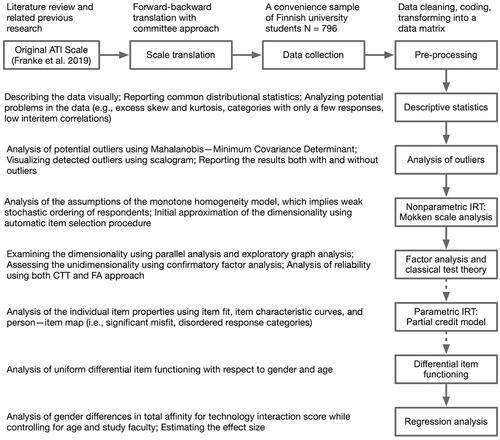
Our analytical process was as follows (Figure 1). We began with descriptive statistics and examined whether the data contained any peculiarities (e.g., excess skew or kurtosis, ceiling or flooring effects, categories without responses). Subsequently, we continued with Mokken scale analysis. It is a convenient nonparametric method making no assumptions about the data distribution while providing an initial assessment of the important scale properties. Mokken scale analysis addresses whether the total score of the scale can be used to order persons with respect to the measured construct. A scale forming a Mokken scale would be a promising candidate for further analysis.

Figure 1. An overview of the analytics scheme.

Next, we used factor analyses for evaluating the structural properties of the scale in detail. The assessment of dimensionality is critical, and it “requires informed judgment that balances statistical information with conceptual plausibility and utility” (Fabrigar & Wegener, 2012, p. 148). The expected number of dimensions is naturally determined in the original scale validation research for an existing scale. However, a new translation and a new cultural context necessitate a new dimensionality assessment.

After the Mokken scale analysis and the factor analysis, we scrutinized the scale further by utilizing the parametric item response theory. As the ability to order persons in their latent variable is an important feature of a scale, we used the partial credit model (PCM) for the analysis because it is the least restrictive parametric IRT model still possessing a more accurate property of stochastic ordering of the latent variable by the total scale score (i.e., SOL by $X_{+}$) (Hemker et al., 1997; Ligtvoet, 2012; van der Ark, 2005). Furthermore, the PCM analysis provided information at the item level. For conciseness, the complemental analysis based on parametric item response theory using PCM is presented in Appendix C.

2.4.1. Descriptive statistics and multivariate outliers

The data were first examined using basic descriptive statistics. Nonnormality is usual in the case of real-world psychological and educational data (Cain et al., 2017). Mardia’s test for multivariate skewness and kurtosis (Mardia, 1970; Mecklin & Mundfrom, 2007) was used to assess whether the data complies with the multivariate normal distribution (McDonald & Ho, 2002). A significant result in Mardia’s test indicates that the data were not complying with multivariate normal distribution. Univariate skewness and kurtosis were assessed using Fisher’s skewness (G₁) and kurtosis (G₂) (Cain et al., 2017; Joanes & Gill, 1998). A scalogram was used to describe the individual response patterns visually (e.g., Massof, 2004).

To detect possible multivariate outliers, we used Mahalanobis–Minimum Covariance Determinant with a breakdown point of 0.25 (MMCD75). As a robust version of the traditional Mahalanobis distance, MMCD75 was suggested to be efficient in detecting outlying values as well as having an acceptable false detection rate (Leys et al., 2018). We analyzed the data with and without the outliers. For transparency, both results are reported when the difference is deemed to be more than negligible or the result is otherwise crucial for assessing the effect of outliers in the data (e.g., measures of association). All possible outliers identified by the MMCD75 method were depicted visually using a scalogram.

2.4.2. Nonparametric item response theory

Models belonging to the field of nonparametric item response theory (NIRT) are data-driven exploratory models, which assume that the relationship between the latent variable and the item score is restricted only by order (Sijtsma, 2005). One such model is the monotone homogeneity model (MHM) for dichotomous (Mokken, 1971, 1997) and polytomous (Molenaar, 1997) data. MHM is also known as the nonparametric graded response model (np-GRM) (Sijtsma & van der Ark, 2020, p. 233) and it is the most general of all well-known IRT models for polytomous data (Hemker et al., 2001; van der Ark & Bergsma, 2010). The general MHM has some desirable psychometric properties in terms of total scale score. Thus, in this paper, we first start our analysis by assessing the applicability of MHM to the collected scale data.

MHM is based on three key assumptions: i) unidimensionality, which means that all items are measuring the same latent variable, ii) local independence, which means that the item scores depend only on the person’s latent variable; and iii) latent monotonicity of the item step response functions (ISRFs), which means that the functions are non-decreasing concerning the latent variable (Sijtsma, 2005; Sijtsma & van der Ark, 2017; van der Ark, 2012). A more strict model, the double monotonicity model (DMM), also assumes invariant item ordering, which means that the scale items can be placed in order with respect to the latent variable (Sijtsma & van der Ark, 2017). Mokken scale analysis (MSA) (Sijtsma et al., 2011; Sijtsma & van der Ark, 2017)) is a set of tools, which can be used to analyze how dichotomous or polytomous scale data meet the assumptions of MHM and DMM. Scale identification in MSA involves examining the applicability of the assumptions in the data, in other words, assessing scalability, local independence, and invariant item ordering of the scale items in addition to the monotonicity of the ISRFs.

Scalability in MSA is based on the coefficient of homogeneity H (Loevinger, 1948; Mokken, 1971) also called as the scalability coefficient (Sijtsma & van der Ark, 2017). Existing scales can be evaluated directly using the inter-item coefficients H_jk, coefficients of the individual items H_j, and the overall coefficient H for the whole scale (Mokken, 1971, 1997). Higher H_j implies better item discrimination and values close to 0 do not discriminate well in terms of the latent variable (Sijtsma & van der Ark, 2017; Straat et al., 2014). Thus, a common approach to decide whether to include items to a scale is to define a threshold value c so that all $H_j>c$. The lowest threshold value traditionally used for considering the inclusion of an item to the scale is $H_j>0.30$

for all items and the excluded items are considered as unscalable (Mokken, 1971; Sijtsma & van der Ark, 2017). For classifying complete scales, $0.30\le H<0.40$ forms a weak Mokken scale, $0.40\le H<0.50$ forms a medium scale, and $H\ge 0.50$ forms a strong scale (Mokken, 1971, p. 185).

Instead of relying on arbitrary threshold values, an automated item selection procedure (AISP) provides a way to examine the scale items’ scalability and dimensionality. AISP is an iterative process, which aims to select items from the initial item bank so that (i) the selected item has a positive covariance with each of the already selected items, (ii) the item has $H_j\ge c$, and (iii) the selected item maximizes the overall H value of the scale with other selected items (Hemker et al., 1995). Instead of selecting a single threshold value c, one suggested approach is to run AISP for a sequence of thresholds (e.g., c = {0.05, 0.10, 0.15, …, 0.60}) (Hemker et al., 1995; Sijtsma & van der Ark, 2017). The examinations of the sequential outcome pattern of AISP can reveal whether the data form one or more scales and whether some items turn out to be unscalable at a certain level of c (Hemker et al., 1995). Two different procedures have been proposed for AISP, Mokken’s procedure (Mokken, 1971, p. 191) and a genetic algorithm (Straat et al., 2013). The two algorithms might yield different results for the same data (Sijtsma & van der Ark, 2017). The minimum sample size for using the AISP procedure depends on the item quality, but at least 250 to 500 responses are needed (Straat et al., 2014).

The scale items’ local independence can be assessed using a procedure based on conditional association (CA). The procedure CA flags items as locally dependent and removes them one by one based on conditional covariances, indices $W^{(1)},W^{(2)}$, and $W^{(3)}$, to identify a locally independent item set (Straat et al., 2016). An item or an item pair is flagged as locally dependent if $W>Q_3+1.5*\mathit{IQR}$, where Q₃ is the third quartile, and IQR is the interquartile range of the empirical W distribution (Straat et al., 2016) (i.e., W is outside of Tukey’s upper inner fence (Tukey, 1977, p. 44)). In this study, we utilized the procedure CA implemented in the mokken package (van der Ark, 2012).

Latent monotonicity means that the item step response function is a nondecreasing function with respect to the latent variable (van der Ark, 2012). In other words, the higher the person’s ability on the latent variable, the higher the probability of scoring cases typical of the higher attribute level (Sijtsma & van der Ark, 2017). Manifest monotonicity—a property observed from the scale data—can be used to assess latent monotonicity using a procedure implemented in the R package mokken (van der Ark, 2007, 2012). The procedure combines respondents to rest score groups based on a selected minimum group size criterion minsize. Manifest monotonicity is assessed based on the probability of belonging to a higher rest score group with respect to a higher latent variable, and violations exceeding a minimum value minvi are considered relevant. For the data in this study, minsize = $N/10$ and minvi = 0.30 were used (van der Ark, 2007).

2.4.3. Factor analysis

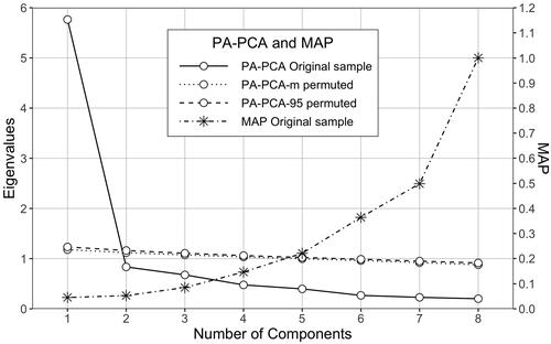
The first step in factor analysis is to assess the dimensionality of the data and decide how many factors to retain. A suggested approach is to use multiple methods to assess the dimensionality of the data and compare their results (Lubbe, 2019). To assess the dimensionality and the number of factors to retain, we used parallel analysis (PA) and minimum average partials (MAP). The parallel analysis compares the structure in the collected data to a structure of randomly sampled data. The number of dimensions in the actual data exceeding the number of dimensions on the random data is retained. PA is often referred to as one of the most accurate and robust rules for determining the dimensionality of the data (Lubbe, 2019), and it performs well in a wide variety of scenarios (e.g., Golino et al., 2020). PA with PCA extraction (PA-PCA, a.k.a., Horn’s PA (Horn, 1965)) using polychoric correlation has been suggested to be suitable for all types of data (Garrido et al., 2013). For PA-PCA, we used a non-parametric version of parallel analysis with column permutation (500 random data sets), polychoric correlation, and quantile thresholds 50% (median, PA-PCA-m) and 95% (PA-PCA-95) (Auerswald & Moshagen, 2019; Buja & Eyuboglu, 1992).

Another promising and recent approach for analyzing the dimensions of psychological constructs is exploratory graph analysis (EGA). EGA draws from the methods behind network psychometrics, which in turn aims to combine different latent variable models and network models (Epskamp et al., 2017, 2018). EGA utilizes partial correlations and the Gaussian graphical model with a clustering algorithm for a weighted network (i.e., Walktrap algorithm) (Golino et al., 2020). EGA is suggested to possess several advantages over more traditional methods. For example, the results of EGA can be interpreted visually instead of interpreting a factor loading matrix, and there is no need to make decisions about the factor rotation (Golino et al., 2020). Two different estimators have been suggested to be used in EGA (Golino et al., 2020): the graphical least absolute shrinkage and selection operator (GLASSO) (Friedman et al., 2008) and the triangulated maximally filtered graph (TMFG) (Massara et al., 2016). The advantage of the EGA-TMFG method is that it does not assume the data to be multivariate normal, and it is suggested to perform at its best with unidimensional data (Golino et al., 2020). Furthermore, total entropy fit index (TEFI) using Von Neuman’s entropy can be used to evaluate the EGA model fit, and lower values of TEFI indicate lower disorder (i.e., better fit) (Golino et al., 2020).

Confirmatory factor analysis (CFA) covers the steps of model specification, estimation, and evaluation (Brown, 2015). The basis for the model specification in our research was the original (a priori) unidimensional model (i.e., Franke et al., 2019). The model estimation was conducted employing polychoric correlation (Holgado-Tello et al., 2010) and robust diagonally weighted least squares (DWLS) estimation with test statistics adjusted in terms of mean and variance (i.e., scale-shifted approach, a.k.a., WLSMV (El-Sheikh et al., 2017)), which is a suggested estimation method for ordinal data (Beauducel & Herzberg, 2006; DiStefano & Morgan, 2014; Foldnes & Grønneberg, 2021; Forero et al., 2009; Li, 2016a, 2016b, 2021).

To describe the goodness of fit of the CFA models, we used the standardized root mean squared residuals (SRMR) as an indicator of the absolute fit, the root mean square error of approximation (RMSEA) as an indicator of the parsimony corrected fit, and the comparative fit index (CFI) and Tucker—Lewis index (TLI) as indicators of the comparative fit. In general, SRMR and RMSEA values closer to zero and CFI and TLI values closer to one are considered as indicators of better fit of the model. Specifically, SRMR is relatively insensitive to different estimators and appropriate to use in the case of ordinal models (Shi & Maydeu-Olivares, 2020). Various suggestions for deriving cut off values and combinational rules for an acceptable model fit can be found in the literature (e.g., TLI or CFI > 0.95 and SRMR < 0.09 (Hu & Bentler, 1999), dynamic fit index (McNeish & Wolf, 2021)); however, no “golden rule” exists (e.g., Greiff & Heene, 2017; Shi et al., 2019).

Furthermore, we conducted a specification search using modification indices (i.e., Lagrange multipliers) to examine the localized areas of strain in the model. Complementing the global model fit assessments based on the goodness-of-fit measures, the modification indices based on the expected parameter change provide insights about the local misspecifications (e.g., Greiff & Heene, 2017). The use of modification indices is exploratory in nature, and the modifications should be based on underlying theoretical assumptions of the model (Brown, 2015, p. 106). CFA was conducted and the modifications were applied based on the expected parameter change and power analysis (Saris et al., 2009) using the R package lavaan (Rosseel, 2012).

We estimated the reliability of the scale from the classical test theory (CTT) and factor analysis points of views. Coefficient α (e.g., Cronbach, 1951) is based on the assumptions of CTT (Lord & Novick, 1968, p. 36–38). The underlying idea in reliability is replicability: the reliability ${\rho }_{XX\prime }$ of a test reflects the degree of linear correlation between two parallel tests having the same formal properties (Sijtsma & Pfadt, 2021). In essence, coefficient α is a lower bound to the reliability (Sijtsma, 2009; Sijtsma & Pfadt, 2021); however, under approximate unidimensionality it is close to reliability ${\rho }_{XX\prime }$ (Sijtsma & Pfadt, 2021). On the other hand, the reliability coefficient ω (e.g., McDonald, 1999, p. 88–90) is based on the concept of a factor analysis (FA) model. As suggested for categorical data, we estimated the reliability following FA approach by using categorical omega ω_c with bias-corrected and accelerated bootstrap confidence interval (Dunn et al., 2014; Kelley & Pornprasertmanit, 2016) implemented in R package MBESS (Kelley, 2007).

2.4.4. Differential item functioning

Differential item functioning (DIF) means that persons having the same level of ability in the latent variable respond differently to the item depending on the persons’ characteristics. For example, if an item exhibits gender-based DIF, it means that men and women with the same ability with respect to the latent variable have different probabilities for response categories. A wide variety of methods have been proposed to detect DIF, but many of them suffer from fundamental issues (e.g., requiring a priori chosen anchor items) (Bechger & Maris, 2015; Yuan et al., 2021). For detecting uniform DIF, we used a recent method utilizing an approach based on the lasso principle, which does not require using anchor items (Schauberger & Mair, 2020). The DIF analysis was executed using R package GPCMlasso (Schauberger, 2019).

2.4.5. Total scale score

When measuring a latent variable using a psychometric scale, the total scale score $X_{+}$—usually calculated as the unweighted sum of all item scores—is assumed to be the proxy of the measured latent variable. Some IRT models have a property called stochastic ordering of the latent variable by $X_{+}$(SOL by $X_{+}$), which implies that a higher total score $X_{+}$ results in a higher expected latent variable value (Hemker et al., 1997). If the data comply with a model having the property of SOL by $X_{+}$, then the simple sum score $X_{+}$ can be used to order respondents in terms of the latent variable (Sijtsma & Hemker, 2000). SOL by $X_{+}$ holds for MHM with dichotomous data (Mokken, 1997; Sijtsma & Hemker, 2000). MHM with polytomous data does not imply SOL by $X_{+}$ (Hemker et al., 1997). However, a property called weak SOL was proposed to apply to MHM with polytomous data, which in turn is argued to justify the ordering of respondents on the latent variable using the total score $X_{+}$ (van der Ark & Bergsma, 2010). MHM for polytomous items does not imply complete person ordering, but it allows for pairwise person ordering (van der Ark et al., 2019). Even though MHM might not be completely satisfactory for the exact ordering of individuals, it can be used to order groups of people using statistics of central tendency (e.g., mean and median) as people with a higher $X_{+}$ have on average a higher ability on the latent variable compared to people with a lower $X_{+}$ (Zwitser & Maris, 2016). The corrected item-total correlation is used to indicate the coherence between an item and the other items in a scale, and it is one of the best methods for item assessment when constructing tests (Zijlmans et al., 2018). The corrected item-total correlation is calculated by correlating the item score with the total scale score without that item. Items with a higher corrected item-total correlations are more desirable (DeVellis, 2017, p. 142).

2.5. Ethical considerations

The research was conducted following the guidelines of the World Medical Association (WMA) Declaration of Helsinki. According to the guidelines of The Finnish National Board on Research Integrity and the research institution where the research was conducted, ethical pre-evaluation or permission was not needed for executing the research. Participation in the research was voluntary. Research and privacy statement was prepared following the GDPR and national legislation. An informed consent was asked before respondents answered the questionnaire. Identifying information (i.e., email address) was asked to enable the voluntary gift card raffle. It was also possible to participate in the research entirely anonymously. The data were anonymized directly after data collection.

3. Results

3.1. Descriptive statistics

First, multivariate outliers were identified using MMCD75 (Leys et al., 2018), and 39 (4.9%) responses were identified as potential outliers. After excluding the outliers, there were n = 757 responses with similar demographic properties as the complete data. We analyzed the data with and without outliers. The results including outliers are interpreted in the text or presented using a marker †. It is worth noting that the distributional properties of the data represent the reponses of this particular convenience sample consisting of relatively young and educated people.

Figure 2 depicts the distributions of answer categories of each scale item without outliers. All answer categories received responses. The least amount of responses were in Completely disagree categories of items ATI8 (n = 20; 2.6%) and ATI9 (n = 14; 1.8%). Table 2 describes the distributional properties of the items without outliers. The effect of the outliers on the distributional properties was negligible. Mardia’s tests for multivariate skewness and kurtosis of the items were significant, which indicated the data deviated from multivariate normal distribution. As expected, the reverse-worded items ATI3, ATI6, and ATI8 were negatively associated with all other items. After reverse-coding the reverse-worded items using linear scaling, all interitem correlations were positive.

Figure 2. Likert responses without outliers. RW items ATI3, ATI6 and ATI8 are not reversed.

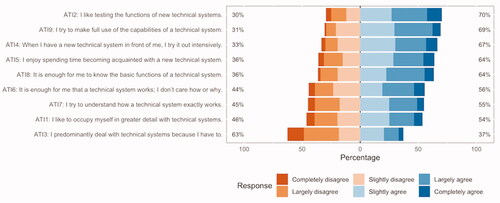
Table 2. Distributional properties of the items without outliers ordered by the mean.

Item	M	SD	Skew G1	Kurtosis G2	SE
ATI9	4.05	1.13	−0.40	−0.39	0.04
ATI2	4.04	1.37	−0.52	−0.57	0.05
ATI3R	4.00	1.40	−0.33	−0.86	0.05
ATI4	3.95	1.26	−0.35	−0.46	0.05
ATI5	3.83	1.36	−0.31	−0.77	0.05
ATI7	3.58	1.37	−0.13	−0.99	0.05
ATI1	3.56	1.38	−0.09	−0.92	0.05
ATI6R	3.25	1.39	0.17	−0.93	0.05
ATI8R	3.07	1.28	0.33	−0.84	0.05

The effect of including outliers was negligible.

Correlations between the items using polychoric correlation ranged between 0.37–0.83 (0.31–0.81^†). The item ATI3R exhibited the weakest association with other items (0.37–0.49, 0.31–0.46^†), however, not as weak as reported in Lezhnina and Kismihók (2020) (0.14–0.26). Heterogeneous interitem correlations could indicate that the items do not capture the latent variable equally well (DeVellis, 2017, p. 55).

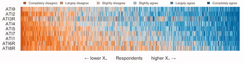
We used a scalogram to depict the variation in the respondents’ response patterns visually. Figure 3 shows all response patterns excluding the outliers. In the figure, the respondents were ordered according to the sum score X₊, and the scale items were ordered according to the item sum score. Thus, the colors depicting the amount of agreeableness would accumulate to the top right corner of the figure. Respectively, the colors depicting the amount of disagreeableness would accumulate to the lower left corner of the figure. Visual inspection showed that especially the item ATI3R exhibited a somewhat irregular response pattern. Appendix Figure D1 depicts the scalogram containing only the outliers identified by the MMCD75 procedure. Several dubious responses can be identified (e.g., extreme and low scorers, contradicting responses) exhibiting ambiguous response patterns. As described above, instead of subjective selection, we removed all outliers suggested by MMCD75 and report results with and without outliers.

Figure 3. Scalogram without outliers (n = 757), respondents ordered by total score, and items ordered by total item sum.

3.2. Mokken scale analysis

We utilized non-parametric item response theory (Sijtsma, 2005), namely the monotone homogeneity model (Mokken, 1971), by applying Mokken scale analysis (Sijtsma & van der Ark, 2017) to the scale data. First, we examined the scalability of the scale items using the coefficient H (Appendix Table B1). After reverse coding the reverse-worded items, all scalability coefficients were positive. For individual items, the values were $0.43<H_j<0.66$ (0.014 < SE < 0.027) exceeding the traditional cutoff value c = 0.3. For item pairs, the values were $0.35<H_{jk}<0.82$. The effect of including outliers was small. Local independence was assessed using conditional association procedure (Straat et al., 2016). Without outliers, all items were found to be locally independent. With outliers, $W^{(1)}$ flagged the item pair ATI7–ATI1 as locally dependent.

We examined the monotonicity of the ISRFs, and there were only six (five^†) violations of manifest monotonicity (all in RW items) using minvi = $N/10$, minvi = 0.03. All violations of manifest monotonicity were non-significant at the level of $\alpha =.05$, which indicates that the assumption of monotonicity holds. However, the data with and without outliers showed significant violations of invariant item ordering. Thus, the data did not support the more strict assumption of the double monotonicity model.

In addition, we used AISP to assess the dimensionality of the scale. When increasing the threshold consecutively using c = {0.05, 0.10, 0.15, …, 0.60}, one would expect to find most or all items assigned to the same scale (Sijtsma & van der Ark, 2017). Both AISP algorithms (i.e., Mokken’s method and the genetic algorithm) produced identical results for data without outliers. With outliers, the algorithms produced slightly different results, and Mokken’s method is reported with outliers (Table 3). The AISP algorithms assigned all items to the same scale without outliers at the level of c = 0.40 and with outliers at the c = 0.35. According to AISP, the RW items were less scalable than other items. The outliers affected the scalability of RW items and ATI7; however, the effect was minimal. In summary, the results of the Mokken scale analysis supported the requirements of MHM (i.e., unidimensionality, monotonicity, and local independence). Furthermore, the Finnish version of the ATI scale formed a strong Mokken scale, which met the criteria of the monotone homogeneity model.

Table 3. The results of the consecutive steps of the automatic item selection process (AISP).

Item	.05	.10	.15	.20	.25	.30	.35	.40	.45	.50	.55	.60
ATI1	1	1	1	1	1	1	1	1	1	1	1	1
ATI2	1	1	1	1	1	1	1	1	1	1	1	1
ATI3R	1	1	1	1	1	1	1	1;0^†	0	0	0	0
ATI4	1	1	1	1	1	1	1	1	1	1	1	1
ATI5	1	1	1	1	1	1	1	1	1	1	1	1
ATI6R	1	1	1	1	1	1	1	1	1	1	1;2^†	2
ATI7	1	1	1	1	1	1	1	1	1	1	1	1;2^†
ATI8R	1	1	1	1	1	1	1	1	1	1;0^†	0;2^†	2;0^†
ATI9	1	1	1	1	1	1	1	1	1	1	1	1

Note. Data with outliers is marked using ^†.

3.3. Factor analysis and classical test theory

3.3.1. Parallel analysis

Figure 4 shows the results of the parallel analysis. PA-PCA supported unidimensional structure because the eigenvalue of the first component in the scale data was higher and the value of the second component was lower than the corresponding values in the parallel simulated data. Two of the smallest values of MAP were 0.045 (0.047^†) and 0.053 (0.049^†). Also, the smallest MAP value suggested a unidimensional structure. The effect of including outliers in the parallel analysis was negligible.

Figure 4. Both MAP and parallel analysis using PCA for the complete data without outliers supported structure with one component.

3.3.2. Exploratory graph analysis

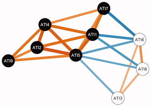
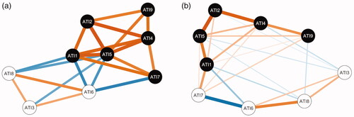
We applied EGA using both GLASSO and TMFG estimation for the data without outliers. The model using TMFG (Figure 5(a)) was chosen as the final model as TMFG was suggested to perform better in case of unidimensional data (Golino et al., 2020) and it also showed a smaller TEFI value (TEFI = −4.97) when compared to the GLASSO estimation (TEFI = −4.57) (Figure 5(b)). Both estimation methods showed similar two-dimensional structures, except that the GLASSO estimation assigned ATI7 to the same dimension with RW items. The structures were identical with the data including outliers, except that the GLASSO estimation assigned also ATI1 to the same dimension with the ATI7 and RW items (Figure 2(a,b)).

Figure 5. EGA for the complete data without outliers using TMFG (a) showed better fit (TEFI = −4.97) supporting two-dimensional structure. Edges represent the partial correlations between items.

3.3.3. Confirmatory factor analysis

We conducted CFA for the original unidimensional a priori model (Model 1). The model without outliers showed a better fit than the model including outliers (Table 4). The post hoc exploratory power analysis of the modification indices suggested adding correlated errors between ATI6R–ATI7, ATI6R–ATI8R, ATI3R–ATI8R, ATI3R–ATI6R, and ATI1–ATI6R. The results reflect a local discrepancy in the model. In other words, the model does not adequately reproduce the relationships of the item pairs mentioned above. Adding correlated errors based on the modification indices can be justified if there is a reason to believe that some of the covariations are due to some common exogenous cause instead of the latent variable (Brown, 2015, p. 157). The common cause for the discrepancy of the RW item pairs could be caused by a common method bias (DiStefano & Motl, 2006; Podsakoff et al., 2003; Woods, 2006) and systematic bias relating to item wording (Dalal & Carter, 2014, p. 117). For the other item pairs (i.e., ATI6R–ATI7 and ATI1–ATI6R), the cause for a local misfit could be their polar opposite wording as polar opposite items could affect on factorial structure (Zhang et al., 2016). Consequently, we applied the modification indices above, and the modified model (Model 2) resulted in an improved and sufficient fit both with and without outliers.

Table 4. The CFA estimates for a priori model (Model 1) and modified model (Model 2) using the data without outliers and with outliers (^†).

	${\chi }^2$	df	$p<$	${\chi }^2$ /df	RMSEA [90% CI]	SRMR	CFI	TLI
Model 1	442.7	27	.001	16.4	0.143 [0.131–0.155]	0.053	0.971	0.961
Model 1^†	568.2	27	.001	21.0	0.159 [0.148–0.170]	0.061	0.958	0.944
Model 2	130.6	22	.001	5.9	0.081 [0.068–0.094]	0.024	0.992	0.988
Model 2^†	222.8	22	.001	10.1	0.107 [0.095–0.120]	0.032	0.984	0.974

3.3.4. Reliability

From the FA point of view, the test score reliability using categorical omega showed high reliability, ω_c = 0.946 (0.927^†), 95% CI [0.926 (0.915^†), 0.944 (0.936^†)]. Also, in terms of CTT, the lower bound to the reliability of the ATI test score using coefficient α showed high reliability estimate, α = 0.915 (0.903^†), 95% CI [0.905 (0.891^†), 0.924 (0.913^†)]. The effect of outliers was minimal.

3.3.5. Differential item functioning

We examined the existence of a uniform DIF concerning age and gender using a regularization approach based on the lasso principle and PCM (Schauberger & Mair, 2020). Only item ATI3R exhibited uniform DIF based on gender, and none of the items showed a DIF concerning age. The results were the same for both data with and without outliers.

3.4. Total scale score

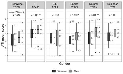
The corrected item-total correlations were adequate ranging between 0.51 (ATI3R) and 0.82 (ATI5). The RW items had the lowest corrected item-total correlations (0.51–0.67). Shapiro-Wilk normality test was significant (W = 0.99, p < .001), indicating that the total score was not normally distributed. However, the histogram and quantile-quantile plot of the total score (Figure 6) showed a shape of an approximately normal distribution. The sample mean (M = 33.3) was close to the center of the scale (C = 31.5). There were no ceiling or flooring effects present. The scale mean for all respondents without outliers was 3.7 (SD = 1.0), for all women 3.5 (SD = 0.97), for all men 4.1 (SD = 0.99), and for a very small sample of non-binary respondents 4.0 (SD = 0.88). Appendix Table B2 shows the descriptive statistics of the total score in different groups. Figure 7 shows the difference in mean ATI scale score between women and men by field of study in this sample. Men showed slightly higher score value than women, specifically and interestingly in the fields of information technology and natural sciences. The results describe the differences in this particular sample and convenience sampling limits the generalizability of the results.

Figure 6. The histogram and the superimposed Q-Q plot of the total ATI scale score without outliers. The total ATI scale range is [9, 54], and the center of the scale is 31.5. The mean and the standard deviation in the figure represent the values from the complete data without outliers.

Figure 7. Difference in mean ATI scale score between genders in different field of studies.

We used hierarchical multiple regression analysis to determine if the addition of gender improved the prediction of the total ATI scale score over and above age and field of study alone. The difference in explained variance between the models with and without gender as an independent variable would indicate the effect of gender on ATI when controlling for age and field of study. After fitting the model, visual inspection of the plot of studentized residuals versus unstandardized predicted values and the quantile-quantile plot did not reveal heteroscedasticity or violations of normality in the full model.

The full regression model regressing the total ATI scale score on gender, age, and field of study was statistically significant, $R^2=0.18,R_{\mathit{adj}}^2=0.17,F(9,739)=17.76,p<.001$. The full model results indicated that when controlling age and faculty, men had 4.6, 95% CI [3.2, 5.9] points higher total ATI scale score (0.51 on the Likert scale). When comparing to a nested model without gender variable, the addition of gender to the prediction of the total ATI scale score led to a statistically significant increase in the coefficient of determination, $\Delta R_{\mathit{adj}}^2=0.05,F(2,739)=22.51,p<.001$. In other words, gender accounted for an additional 5% of the variance in the data and the relating effect size of gender on ATI score, f² = 0.06, 95% CI [0.05, 0.07], was small when using conventional criteria (Cohen, 1988, p. 413). The effect of outliers on the effect size was negligible.

In a meta-analysis by Cai et al. (2017), the overall weighted effect size relating to gender and attitudes toward technology (i.e., men having favorable attitudes towards technology) across all 87 reported studies was found to be small. On the other hand, when comparing group means between men and women using a quota sample, Franke et al. (2019) identified a large effect in ATI (i.e., men having a higher ATI score). Naturally, the findings relating to gender differences in our study can not be generalized due to sampling method and sample characteristics. However, the results are a one indication that the translated scale is able to capture differences between groups.

4. Discussion

Affinity for technology interaction (ATI) scale is a psychometric instrument used to quantify the tendency of a person to “actively approach interaction with technical systems or, rather, tend to avoid intensive interaction with new systems” (Franke et al., 2019). This research presented a psychometric analysis and properties of a Finnish version of the scale. The main aims of the analyses were to assess the evidence concerning the scale’s internal structure (i.e., dimensionality and the functioning of the individual items). Furthermore, we examined its ability to capture differences and similarities in ATI among students in higher education by gender and field of study.

The Finnish translation was conducted using a professional forward-backward translation process with committee approach (Sousa & Rojjanasrirat, 2011). Data were collected using convenience sampling, and the respondents were university students from six different faculties in a Finnish university. Our comprehensive analysis involved factor analysis and analyses based on both parametric and non-parametric IRT. In addition, we analyzed the data in terms of outliers, and the results were reported both with and without outliers. In general, the outliers seemed to hinder the properties of the scale, but the effect was minimal.

Unidimensionality is a convenient feature of a psychometric scale and the original scale has been deemed unidimensional in previous studies (Franke et al., 2019; Lezhnina & Kismihók, 2020). For the translated version in this study, parallel analyses using traditional PA-PCA and MAP supported a unidimensional structure. On the other hand, a network psychometrics approach using EGA showed a two-dimensional structure where the RW items separated as a second dimension. Post hoc analysis of the unidimensional CFA model showed similar structural indications as EGA. As a result, it can be stated that RW items and both items ATI1 and ATI7 showed some discrepancy concerning unidimensionality. The discrepancy from the unidimensionality could be caused by a common method bias relating to RW items. It is well-known in the literature that the RW items in a scale can hinder the unidimensional structure (Boley et al., 2020; Suárez-Álvarez et al., 2018). Furthermore, they can affect response patterns (Baumgartner et al., 2018; Woods, 2006; Zhang et al., 2016) and mixed scales could also be less reliable and have more measurement error (Dalal & Carter, 2014; Schriesheim et al., 1991).

In general, however, the translated version showed at least moderate fit to the unidimensional model even though the cut-off values for the fit indices for ordinal CFA are not yet settled in the research literature. Essential unidimensionality means that the scale consists of minor dimensions still tapping the same latent variable (Slocum-Gori & Zumbo, 2011). Thus, the translated version could be considered as essentially unidimensional. From the both CTT and FA point of view, the translated scale showed excellent reliability estimates.

The Mokken scale analysis based on the non-parametric IRT showed that the translated scale’s data fitted well to the MHM. In other words, the scale conformed with the requirements of unidimensionality, monotonicity, and local independence. Furthermore, the original ATI scale was found to support also invariant item ordering (Lezhnina & Kismihók, 2020). However, the Finnish version in our research did not support invariant item ordering indicating that the items do not have a specific ordering based on the item difficulty. The translated version formed a strong Mokken scale which means it supports at least the weak SOL by X₊. Thus, it is possible to form a composite total scale score that can be used to order persons on the latent variable (van der Ark & Bergsma, 2010).

The possibility to use the total scale score to differentiate persons concerning their latent variable (SOL by X₊) and the lack of uniform differential item functioning allowed us to advance our analysis by examining the gender differences relating to ATI. We used multiple regression to assess the gender difference in ATI while controlling for the known variables, age and the faculty the respondent was studying in. The results showed that men exhibited slightly more affinity towards technology interaction than women. Specifically, the difference in the sample among the IT students was interesting as the particular subsample was more balanced in terms of gender than other subsamples. The findings can be considered as indications of the differential validity of the scale. While the actual effect size relating to gender was small, a similar difference between genders has been identified in the research literature, and the effect size in this study was comparable to findings in a recent meta-review by Cai et al. (2017). Naturally, it is worth questioning if the difference is large enough to have any practical significance (c.f., Whitley, 1997). However, as the technical systems gain more and more traction and influence in our lives, even a small effect can become significant and meaningful over time. Technological agency would be an essential characteristic that enables and promotes equal participation in various fields of life. Thus, it is of the utmost importance to have valid and cross-cultural instruments to assess the different personal stances towards technology and technical systems.

Our study presented several contributions. Firstly, to our knowledge, this is the first comprehensively analyzed translation besides the original ATI scale versions (c.f., Franke et al., 2019) and the first Finnish psychometric scale for measuring affinity for technology interaction. Secondly, as the previous research has analyzed the ATI scale using factor analysis and non-parametric IRT methods (Franke et al., 2019; Lezhnina & Kismihók, 2020), our analysis utilized also parametric IRT methods using PCM. Lastly, we provided an estimate of the gender effect relating to the affinity for technology interaction.

4.1. Limitations and future research

There are limitations in our study that need to be considered. Using an online questionnaire as a medium could be a source of common method bias (Podsakoff et al., 2003). Data were collected from university students having secondary education backgrounds and who pursued at least a bachelor’s degree in their studies. Also, the sample consisted of mostly relatively young people. The sample characteristics mentioned above limit the generalizability of the results with respect to the general population, which is the population of interest of the ATI scale. Specifically, the results concerning the gender differences in ATI can only be applied to the population used in this research (i.e., Finnish university students).

However, it is notable that the fairly large sample covered a broad range of fields of study, and thus it can be seen as sufficiently representing Finnish university students. The translated version of the scale and the results presented here can be useful in research (e.g., educational technology, social media use, technology adoption) targeting university students. Considering the solid results, simple language used in the scale, and the nature of the construct, one could assume that the internal structure of the translated scale in the general population could follow the results presented here. The promising results presented in this study should encourage researchers to conduct more extensive studies. Future research should complement the findings of this research by examining the properties of the translated scale version and gender differences among older people and people with more diverse educational backgrounds, using samples representing the general population, and using other mediums for provisioning the questionnaire.

In general, results concerning gender-based differences in affinity for technology interaction should be treated with caution. The threat of a stereotypical interpretation is important to consider as it can have detrimental effects in various situations (e.g., Barber, 2020; Cadaret et al., 2017; Doyle & Thompson, 2021). Thus, it is worth noting that research examining gender-based differences has the potential to advance unfounded and stereotypical beliefs if not conducted with rigor and interpreted with care. On the other hand, it is essential to examine the differences, for example, from the equity point of view. For that purpose, functional measurement instruments are valuable assets.

We aimed to conduct an accurate and thorough translation; however, in a cross-cultural research, the complete equivalence between different languages is challenging to achieve. Thus, the presented Finnish translation should be examined in different contexts in future research. Furthermore, we did not assess the relationship of ATI with other similar constructs as there is a limited resource of related and validated psychometric scales in Finnish. Thus, future studies should examine the relationships of ATI with similar constructs within a nomological network.

We used correlated errors to modify the CFA model, which can be problematic (Hermida, 2015). Instead, another approach would be to examine the effect of the reverse-worded items using a method factor (DiStefano & Motl, 2006). In general, the use of reverse-worded items in the first place is a controversial topic, and future studies should address the issue of how different types of reverse-worded items affect the factor structure (Zhang et al., 2016). Furthermore, the item ATI3R exhibiting lower qualities would need to be assessed critically and possibly revised as was also noted in a previous study (c.f., Lezhnina & Kismihók, 2020).

5. Conclusion

We analyzed the psychometric properties of a forward-backward translated Finnish version of the affinity for technology interaction (ATI) scale. The analysis utilized factor analysis, non-parametric IRT, and parametric IRT. To conclude, the Finnish version of the ATI scale showed solid psychometric properties. Furthermore, the scale proved to be essentially unidimensional, having high reliability estimates, and forming a strong Mokken scale. The scale also showed differential validity by identifying a gender difference with respect to the measured construct: men showed slightly more affinity towards technology among the respondents in the sample; however, the effect size was small.

Disclosure statement

No potential conflict of interest was reported by the author(s).

Additional information

Notes on contributors

Ville Heilala

Ville Heilala is a doctoral researcher at the Faculty of Information Technology at the University of Jyväskylä. He holds two Master's degrees, one in education and one in computer science. His research relates to understanding human learning using computational methods.

Riitta Kelly

Riitta Kelly is an English teacher at the Centre for Multilingual Academic Communication, University of Jyväskylä, Finland. She is also a doctoral researcher in Applied Linguistics at the University of Jyväskylä.

Mirka Saarela

Mirka Saarela is a research fellow at the Faculty of Information Technology at the University of Jyväskylä. Her research interests combine machine learning, explainable artificial intelligence, cognitive computing, and education.

Päivikki Jääskelä

Päivikki Jääskelä is an Adjunct Professor and a Senior Researcher at the Finnish Institute for Educational Research at the University of Jyväskylä, Finland. Her research focuses on university student agency, learner-centered pedagogy, and teacher development in higher education.

Tommi Kärkkäinen

Tommi Kärkkäinen has been serving as a full professor of Mathematical Information Technology at the Faculty of Information Technology at the University of Jyväskylä since 2002. He has led almost 50 R&D projects, supervised over 50 Ph.D. students, and published over 180 peer-reviewed articles.

Notes

1 Affinity for Technology Interaction Scale https://ati-scale.org/

Appendix A. Translations of the introductory text and Likert options

The original ATI scale, the items, and the introductory text can be found from the original scale developers’ article (Franke et al., 2019) and from their website.

Introductory text

“Kysymme sinulta teknisten järjestelmien käyttämisestä. Tekninen järjestelmä viittaa tässä yhteydessä kaikkiin appeihin, sovelluksiin ja myös varsinaisiin laitteisiin (esim. kännykkä, tietokone, televisio, auton navigaattori). Ole hyvä ja kerro missä määrin olet samaa tai eri mieltä seuraavien väitteiden kanssa.”

Likert options

täysin eri mieltä (1), enimmäkseen eri mieltä (2), hieman eri mieltä (3), hieman samaa mieltä (4), enimmäkseen samaa mieltä (5), täysin samaa mieltä (6)

Appendix B. Properties of the scale items and the total scale score

Table B1. Coefficients of homogeneity for item pairs H_jk and individual items H_j without outliers and with outliers^(†).

Item	Hjk	$H_{jk}$^†	Hj (SE)	Hj (SE)^†
ATI1	0.43–0.80	0.39–0.76	0.66 (0.014)	0.62 (0.016)
ATI2	0.45–0.82	0.42–0.80	0.64 (0.016)	0.60 (0.017)
ATI3R	0.35–0.47	0.30–0.45	0.43 (0.027)	0.40 (0.027)
ATI4	0.47–0.81	0.42–0.78	0.64 (0.015)	0.60 (0.017)
ATI5	0.47–0.82	0.45–0.80	0.66 (0.014)	0.62 (0.016)
ATI6R	0.44–0.67	0.39–0.65	0.56 (0.020)	0.52 (0.022)
ATI7	0.35–0.67	0.30–0.65	0.58 (0.018)	0.54 (0.020)
ATI8R	0.46–0.57	0.42–0.57	0.52 (0.023)	0.48 (0.024)
ATI9	0.38–0.68	0.34–0.65	0.56 (0.021)	0.51 (0.022)

Homogeneity of the whole scale was H = 0.58 (0.54†); SE = 0.015 (0.016†).

Table B2. Total ATI scale score in different groups based on gender and faculty.

Group	n	M/9	M	SD	min	max	G1	G2	SE
All	757	3.7	33.3	9.2	9	54	−0.16	−0.55	0.34
Gender: Women	494	3.5	31.2	8.7	9	52	0.00	−0.50	0.39
Gender: Nonbinary	6	4.0	36.0	7.9	23	44	−0.75	0.32	3.24
Gender: Men	251	4.1	37.3	8.9	9	54	−0.62	0.18	0.56
Faculty: Hum & Soc.Sci	103	3.3	29.7	9.2	10	49	0.02	−0.88	0.90
Faculty: Sports	106	3.3	29.9	8.0	14	51	0.31	0.18	0.78
Faculty: Edu	85	3.4	30.6	8.8	9	51	0.00	−0.16	0.95
Faculty: Natural	162	3.6	32.6	9.5	9	53	−0.17	−0.56	0.75
Faculty: Business	76	3.8	33.8	8.6	11	50	−0.33	0.16	0.99
Faculty: Other	11	4.0	35.7	12.7	15	54	−0.20	−1.08	3.84
Faculty: IT	214	4.2	38.2	7.7	17	53	−0.40	−0.40	0.52

M is the mean of the composite sum score and M/9 is the mean Likert value.

Appendix C. Partial credit model

Parametric item response theory

The partial credit model (PCM) (Masters, 1982)—an extension of the dichotomous Rasch model for polytomous data—is the simplest of all polytomous IRT models widely used in various measurement and assessment scenarios (Masters, 2016, p. 110). Bond et al. (2020, p. 238) define a Rasch model as “a theoretical mathematical description of how fundamental measurement should operate with social/psychological variables”. They continue that “no real, empirical data will ever fit Rasch’s theoretical ideal,” however, the question is more about how closely the model supports the measurement decisions one wants to make (Bond et al., 2020). One important decision a researcher usually wants to make is whether the respondents can be ordered based on their total score. While PCM is a strict model, it is the least strict of models that still have the property of stochastic ordering of latent variable by the total scale score (i.e., SOL by X₊) (Hemker et al., 1997; Ligtvoet, 2012; Sijtsma & Hemker, 2000; van der Ark, 2005). PCM has been used to analyze scales relating to, for example, attitudes (e.g., Aghekyan, 2020), technology interaction (e.g., Makransky et al., 2017), and behavioral intent (e.g., Chen & Jin, 2020).

PCM estimates two parameters: the ability of the person in the latent variable and the item difficulty representing the locations of the item at a point in the latent variable continuum where it is equally likely to choose either of the extreme categories (Masters, 2016, p. 111). Another characteristic of PCM is that the category thresholds are allowed to vary between items, which in turn can give valuable information about the functioning of the response categories between items (Wetzel & Carstensen, 2014). The PCM model was fitted in R using eRm package (Mair & Hatzinger, 2007b) and conditional maximum-likelihood (CLM) procedure, which has mathematical and epistemological advantages (Mair & Hatzinger, 2007a).

Unidimensionality was assessed using principal component analysis of residuals (PCAR). Under unidimensionality, it is expected that the partial credit model explains all the variance in the data, and the residuals represent random noise. Thus, unidimensionality could be supported if all eigenvalues obtained from the PCA of the residuals are less than two and there are no contrasting item loadings on the first component (Bond et al., 2020, p. 254). Local dependency (LD) was evaluated using Q₃ statistics, which is the Pearson correlation between the raw item residuals (Yen, 1984). The difference between the largest observed correlation with the average of the observed correlations denoted as Q_3,* greater than 0.20 could indicate LD (Christensen et al., 2017).

The goodness of fit at the item level was assessed using unweighted mean-square (i.e., outfit) and weighted mean-square (i.e., infit) statistics. Optimal infit and outfit values are close to 1.0, whereas statistically significant values greater than 1.0 indicate underfit (i.e., unpredictability and excess variation in the model), and values less than 1.0 indicate overfit (i.e., deterministic response patterns and less variation in the model) (Bond et al., 2020, p. 241). Overfitting can occur, for example, in the case of item redundancy, and it can cause smaller standard errors, inflated reliability, and local dependency (Bond et al., 2020, p. 241). On the other hand, underfit degrades the measurement quality and is in practice more important to diagnose than overfit (Bond et al., 2020, p. 241). Outfit and infit statistics were calculated based on the conditional residuals (Müller, 2020b) using iarm package (Müller, 2020a).

We examined the category probability curves visually to find out possible disordered categories (i.e., reversed deltas or disordered thresholds). The ordering of category thresholds should follow the ordering of the actual response categories. Disordering of the categories can occur, for example, when a category is not the most likely category at any point along the latent variable (Wetzel & Carstensen, 2014). Disordered categories could indicate dependence among the underlying items; however, rash judgments should be avoided as disordering does not necessarily imply that the item is not functioning as expected (Adams et al., 2012). Another visual representation, person-item map (a.k.a, Wright map), depicts the respondents in terms of their ability and items in terms of their location and thresholds along the latent variable continuum depicted as logit scale (Bond et al., 2020). Thus, a person-item map can be used to evaluate, for example, ordering the response categories and the coverage of the items along with the latent variable.

Results

All results for PCM were similar with and without outliers, and results without outliers are reported here. In the post-hoc analysis, the assumption of unidimensionality was assessed using PCA of the residual correlations. The largest eigenvalue was 2.19, which was slightly greater than the suggested threshold value of 2. Further examination showed contrasting item loadings. RW items and ATI7 showed negative loadings, and all other items showed positive loadings on the largest component. The results indicated that the residuals possibly contained unexplained variance, which would compromise the assumption of unidimensionality from the PCM point of view. Residual correlations (${\overline{Q}}_3$ = −0.12, $Q_{3,sd}$ = 0.16, $Q_{3,\mathit{min}}$ = −0.36, $Q_{3,\mathit{max}}$ = 0.23, $Q_{3,*}$ = 0.35) indicated the existence of local dependency. Seven item pairs out of 36 exhibited $Q_{3,*}>0.20$, and two item pairs, ATI2–ATI4 and ATI2–ATI5, had $Q_{3,*}>0.30$. The effect of including outliers was minimal for both assessing unidimensionality and the local dependency.

Item fit indices (Table C1) indicated significant outfit and infit for all other items except ATI6R, ATI7, and ATI9. Significant overfit could be expected because of item content similarity. However, only items ATI3R and ATI8R showed significant underfit, which can degrade the measurement results (Bond et al., 2020, p. 241). For the item ATI3R, the misfit was extreme, indicating unpredictability and excess variation. The unpredictable pattern of the item ATI3R was also noticeable in the scalogram (Figure 3) and in other previous analyses.

Table C1. Item fit indices of the PCM ordered by the item location (δ_i).

Item	δi	Outfit	Infit
ATI9	0.25	1.06	1.03
ATI3R	0.44	1.81***	1.71***
ATI2	0.47	0.79**	0.79**
ATI4	0.50	0.75***	0.74***
ATI5	0.67	0.69***	0.66***
ATI7	0.99	1.05	1.02
ATI1	1.00	0.72***	0.70***
ATI6R	1.32	1.12	1.12
ATI8R	1.62	1.29***	1.24***

Infit and outfit SE = 0.05 for all items.

Note. Bonferroni adjusted.

${}^{***}$p < 0.001, ${}^{**}$p < 0.01.

Items ATI1, ATI4, ATI8R, and ATI9 showed a plain and ordered category structure (Appendix Figure C1). On the other hand, items ATI2, ATI3R, and ATI5 showed disordered thresholds between two adjacent categories (Appendix Figure C2), and items ATI6R and ATI7 showed one extremely narrow category. Notably, the middle response categories Slightly disagree and Slightly agree showed disordering or highly narrow range in the latent variable (Appendix Figure C3), indicating it was more probable to prefer the extreme categories.

Figure C1. Item characteristic curve of the item ATI4 showed an ordered category structure. Similar ordering was found in items ATI1, ATI8R, and ATI9.

Figure C2. Item characteristic curve of the item ATI2 showed a slightly disordered category structure. Similar ordering was found in items ATI3R and ATI5.

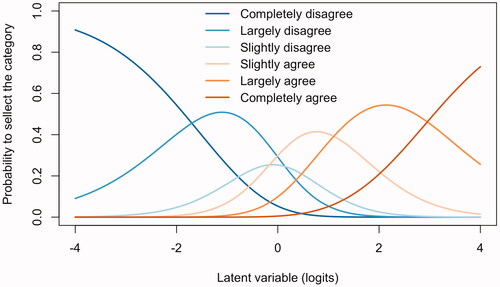
Figure C3. Person-item map of the PCM where items are ordered based on their location. Numbered circles represent the intersection points of adjacent item characteristic curves. Asterisk on the right marginal marks the items exhibiting category disordering.

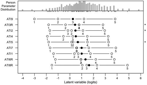
The person-item map showed that the items cover a wide range of the latent variable continuum (Appendix Figure C3). Items ATI4 and ATI9 showed relatively evenly distributed category thresholds. Item ATI8R proved to be the most challenging item to agree with, providing information from the higher end of the continuum. Especially, item ATI9 showed several desirable properties: it covers a wide range of the latent variable with ordered and relatively equal thresholds, it has a central location in the middle of the continuum, and its item fit statistics are adequate.

Appendix D. Results for data including outliers

Figure D1. Scalogram containing only outliers (n = 39) suggested by MMCD75, respondents ordered by total score, and items ordered by total item sum.

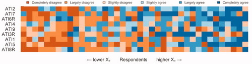
Figure D2. EGA for the complete data including outliers.

References

- Adams, R. J., Wu, M. L., & Wilson, M. (2012). The rasch rating model and the disordered threshold controversy. Educational and Psychological Measurement, 72(4), 547–573. https://doi.org/10.1177/0013164411432166
- Aghekyan, R. (2020). Validation of the SIEVEA instrument using the rasch analysis. International Journal of Educational Research, 103, 101619. https://doi.org/10.1016/j.ijer.2020.101619
- Alabdullatif, H., & Velázquez-Iturbide, J. Á. (2020). Personality traits and intention to continue using massive open online courses (ICM) in Spain: The mediating role of motivations. International Journal of Human–Computer Interaction, 36(20), 1953–1967. https://doi.org/10.1080/10447318.2020.1805873
- Ali, M. A., Alam, K., Taylor, B., & Rafiq, S. (2020). Does digital inclusion affect quality of life? Evidence from Australian household panel data. Telematics and Informatics, 51, 101405. https://doi.org/10.1016/j.tele.2020.101405
- American Educational Research Association, American Psychological Association, & National Council on Measurement in Education (2014). Standards for educational and psychological testing. American Educational Research Association.
- Attig, C., & Franke, T. (2019). I track, therefore I walk – exploring the motivational costs of wearing activity trackers in actual users. International Journal of Human-Computer Studies, 127, 211–224. https://doi.org/10.1016/j.ijhcs.2018.04.007
- Auerswald, M., & Moshagen, M. (2019). How to determine the number of factors to retain in exploratory factor analysis: A comparison of extraction methods under realistic conditions. Psychological Methods, 24(4), 468–491. https://doi.org/10.1037/met0000200
- Barber, S. J. (2020). The applied implications of Age-Based stereotype threat for older adults. Journal of Applied Research in Memory and Cognition, 9(3), 274–285. https://doi.org/10.1016/j.jarmac.2020.05.002
- Baumgartner, H., Weijters, B., & Pieters, R. (2018). Misresponse to survey questions: A conceptual framework and empirical test of the effects of reversals, negations, and polar opposite core concepts. Journal of Marketing Research, 55(6), 869–883. https://doi.org/10.1177/0022243718811848
- Beauducel, A., & Herzberg, P. Y. (2006). On the performance of maximum likelihood versus means and variance adjusted weighted least squares estimation in CFA. Structural Equation Modeling: A Multidisciplinary Journal, 13(2), 186–203. https://doi.org/10.1207/s15328007sem1302_2
- Beaunoyer, E., & Guitton, M. J. (2021). Cyberthanathology: Death and beyond in the digital age. Computers in Human Behavior, 122, 106849. https://doi.org/10.1016/j.chb.2021.106849
- Bechger, T. M., & Maris, G. (2015). A statistical test for differential item pair functioning. Psychometrika, 80(2), 317–340. https://doi.org/10.1007/s11336-014-9408-y
- Boelhouwer, A., Beukel, A. P. V. D., van der Voort, M. C., Verwey, W. B., & Martens, M. H. (2020). Supporting drivers of partially automated cars through an adaptive digital In-Car tutor. Information, 11(4), 185. https://doi.org/10.3390/info11040185
- Boley, B. B., Bynum Boley, B., Jordan, E., & Woosnam, K. M. (2020). Reversed polarity items in tourism scales: Best practice or dimensional pitfall? Current Issues in Tourism, 24(4), 1–13. https://doi.org/10.1080/13683500.2020.1774517
- Bond, T., Yan, Z., & Heene, M. (2020). Applying the Rasch model: Fundamental measurement in the human sciences (4th ed.). Routledge.
- Brislin, R. W., Lonner, W. J., & Thorndike, R. M. (1973). Cross-cultural research methods. John Wiley & Sons.
- Brown, T. A. (2015). Confirmatory factor analysis for applied research (2nd ed.). Guilford Publications.
- Buja, A., & Eyuboglu, N. (1992). Remarks on parallel analysis. Multivariate Behavioral Research, 27(4), 509–540. https://doi.org/10.1207/s15327906mbr2704_2
- Caci, B., Scrima, F., Tabacchi, M. E., & Cardaci, M. (2019). The reciprocal influences among motivation, personality traits, and game habits for playing pokémon GO. International Journal of Human–Computer Interaction, 35(14), 1303–1311. https://doi.org/10.1080/10447318.2018.1519167
- Cacioppo, J. T., & Petty, R. E. (1982). The need for cognition. Journal of Personality and Social Psychology, 42(1), 116–131. https://doi.org/10.1037/0022-3514.42.1.116
- Cacioppo, J. T., Petty, R. E., Feinstein, J. A., & Jarvis, W. B. G. (1996). Dispositional differences in cognitive motivation: The life and times of individuals varying in need for cognition. Psychological Bulletin, 119(2), 197–253. https://doi.org/10.1037/0033-2909.119.2.197
- Cadaret, M. C., Hartung, P. J., Subich, L. M., & Weigold, I. K. (2017). Stereotype threat as a barrier to women entering engineering careers. Journal of Vocational Behavior, 99, 40–51. https://doi.org/10.1016/j.jvb.2016.12.002
- Cai, Z., Fan, X., & Du, J. (2017). Gender and attitudes toward technology use: A meta-analysis. Computers & Education, 105, 1–13. https://doi.org/10.1016/j.compedu.2016.11.003
- Cain, M. K., Zhang, Z., & Yuan, K.-H. (2017). Univariate and multivariate skewness and kurtosis for measuring nonnormality: Prevalence, influence and estimation. Behavior Research Methods, 49(5), 1716–1735. https://doi.org/10.3758/s13428-016-0814-1
- Cameron, J. J., & Stinson, D. A. (2019). Gender (mis)measurement: Guidelines for respecting gender diversity in psychological research. Social and Personality Psychology Compass, 13(11), e12506. https://doi.org/10.1111/spc3.12506
- Cha, E.-S., Kim, K. H., & Erlen, J. A. (2007). Translation of scales in cross-cultural research: issues and techniques. Journal of Advanced Nursing, 58(4), 386–395. https://doi.org/10.1111/j.1365-2648.2007.04242.x
- Chen, J. V., Widjaja, A. E., & Yen, D. C. (2015). Need for affiliation, need for popularity, Self-Esteem, and the moderating effect of big five personality traits affecting individuals’ Self-Disclosure on facebook. International Journal of Human-Computer Interaction, 31(11), 815–831. https://doi.org/10.1080/10447318.2015.1067479
- Chen, L.-M., & Jin, K.-Y. (2020). Development and validation of the willingness to intervene in bullying scale. The British Journal of Educational Psychology, 90(Suppl 1), 224–239. https://doi.org/10.1111/bjep.12319
- Christensen, K. B., Makransky, G., & Horton, M. (2017). Critical values for yen’s q3: Identification of local dependence in the rasch model using residual correlations. Applied Psychological Measurement, 41(3), 178–194.
- Cohen, J. (1988). Statistical power analysis for the behavioral sciences (2nd ed.). Lawrence Erlbaum.
- Cranmer, E. E., Han, D.-I. D., Gisbergen, M. V., & Jung, T. (2021). Esports matrix: Structuring the esports research agenda. Computers in Human Behavior, 117, 106671. https://doi.org/10.1016/j.chb.2020.106671
- Cronbach, L. J. (1951). Coefficient alpha and the internal structure of tests. Psychometrika, 16(3), 297–334. https://doi.org/10.1007/BF02310555
- Dalal, D. K., & Carter, N. T. (2014). Negatively worded items negatively impact survey research. In C. E. Lance & R. J. Vandenberg (Eds.), More statistical and methodological myths and urban legends (pp. 112–132). Routledge.
- DeVellis, R. F. (2017). Scale development: Theory and applications (4th ed.). SAGE Publications.
- DiStefano, C., & Morgan, G. B. (2014). A comparison of diagonal weighted least squares robust estimation techniques for ordinal data. Structural Equation Modeling: A Multidisciplinary Journal, 21(3), 425–438. https://doi.org/10.1080/10705511.2014.915373
- DiStefano, C., & Motl, R. W. (2006). Further investigating method effects associated with negatively worded items on Self-Report surveys. Structural Equation Modeling: A Multidisciplinary Journal, 13(3), 440–464. https://doi.org/10.1207/s15328007sem1303_6
- Doyle, R. A., & Thompson, A. E. (2021). The influence of stereotype threat and implicit theories of emotion on gender differences in emotional intelligence. The Journal of Men’s Studies, 29(2), 131–155. https://doi.org/10.1177/1060826520920878
- Dunn, T. J., Baguley, T., & Brunsden, V. (2014). From alpha to omega: a practical solution to the pervasive problem of internal consistency estimation. British Journal of Psychology (London, England : 1953), 105(3), 399–412. https://doi.org/10.1111/bjop.12046
- Edison, S. W., & Geissler, G. L. (2003). Measuring attitudes towards general technology: Antecedents, hypotheses and scale development. Journal of Targeting, Measurement and Analysis for Marketing, 12(2), 137–156. https://doi.org/10.1057/palgrave.jt.5740104
- El-Sheikh, A. A., Abonazel, M. R., & Gamil, N. (2017). A review of software packages for structural equation modeling: A comparative study. Applied Mathematics and Physics, 5(3), 85–94.
- Epskamp, S., Maris, G. K. J., Waldorp, L. J., & Borsboom, D. (2018). Network psychometrics. In P. Irwing, T. Booth, & D. J. Hughes (Eds.), The Wiley handbook of psychometric testing: A multidisciplinary reference on survey, scale and test development (pp. 953–986). Wiley.
- Epskamp, S., Rhemtulla, M., & Borsboom, D. (2017). Generalized network psychometrics: Combining network and latent variable models. Psychometrika, 82(4), 904–927. https://doi.org/10.1007/s11336-017-9557-x
- Fabrigar, L. R., & Wegener, D. T. (2012). Exploratory factor analysis. Oxford University Press.
- Fleischhauer, M., Enge, S., Brocke, B., Ullrich, J., Strobel, A., & Strobel, A. (2010). Same or different? Clarifying the relationship of need for cognition to personality and intelligence. Personality & Social Psychology Bulletin, 36(1), 82–96. https://doi.org/10.1177/0146167209351886
- Foldnes, N., & Grønneberg, S. (2021). The sensitivity of structural equation modeling with ordinal data to underlying non-normality and observed distributional forms. Psychological Methods, 1–11. Advance online publication. https://doi.org/10.1037/met0000385
- Forero, C. G., Maydeu-Olivares, A., & Gallardo-Pujol, D. (2009). Factor analysis with ordinal indicators: A monte carlo study comparing DWLS and ULS estimation. Structural Equation Modeling: A Multidisciplinary Journal, 16(4), 625–641. https://doi.org/10.1080/10705510903203573
- Franke, T., Attig, C., & Wessel, D. (2019). A personal resource for technology interaction: Development and validation of the affinity for technology interaction (ATI) scale. International Journal of Human–Computer Interaction, 35(6), 456–467. https://doi.org/10.1080/10447318.2018.1456150
- Friedman, J., Hastie, T., & Tibshirani, R. (2008). Sparse inverse covariance estimation with the graphical lasso. Biostatistics (Oxford, England), 9(3), 432–441. https://doi.org/10.1093/biostatistics/kxm045
- Garrido, L. E., Abad, F. J., & Ponsoda, V. (2013). A new look at Horn’s parallel analysis with ordinal variables. Psychological Methods, 18(4), 454–474. https://doi.org/10.1037/a0030005
- Golino, H., Moulder, R. G., Shi, D., Christensen, A. P., Garrido, L. E., & Nieto, M. D. (2020). Entropy fit indices: New fit measures for assessing the structure and dimensionality of multiple latent variables. Multivariate Behavioral Research, 56(6), 874–902. https://doi.org/10.1080/00273171.2020.1779642
- Golino, H., Shi, D., Christensen, A. P., Garrido, L. E., Nieto, M. D., Sadana, R., Thiyagarajan, J. A., & Martinez-Molina, A. (2020). Investigating the performance of exploratory graph analysis and traditional techniques to identify the number of latent factors: A simulation and tutorial. Psychological Methods, 25(3), 292–320. https://doi.org/10.1037/met0000255
- Greiff, S., & Heene, M. (2017). Why psychological assessment needs to start worrying about model fit. European Journal of Psychological Assessment, 33(5), 313–317. https://doi.org/10.1027/1015-5759/a000450
- Hemker, B. T., Andries van der Ark, L., & Sijtsma, K. (2001). On measurement properties of continuation ratio models. Psychometrika, 66(4), 487–506. https://doi.org/10.1007/BF02296191
- Hemker, B. T., Sijtsma, K., & Molenaar, I. W. (1995). Selection of unidimensional scales from a multidimensional item bank in the polytomous mokken I RT model. Applied Psychological Measurement, 19(4), 337–352. https://doi.org/10.1177/014662169501900404
- Hemker, B. T., Sijtsma, K., Molenaar, I. W., & Junker, B. W. (1997). Stochastic ordering using the latent trait and the sum score in polytomous IRT models. Psychometrika, 62(3), 331–347. https://doi.org/10.1007/BF02294555
- Hermida, R. (2015). The problem of allowing correlated errors in structural equation modeling: concerns and considerations. Computational Methods in Social Sciences, 3(1), 5–17.
- Holgado-Tello, F. P., Chacón-Moscoso, S., Barbero-García, I., & Vila-Abad, E. (2010). Polychoric versus Pearson correlations in exploratory and confirmatory factor analysis of ordinal variables. Quality & Quantity, 44(1), 153–166. https://doi.org/10.1007/s11135-008-9190-y
- Horn, J. L. (1965). A rationale and test for the number of factors in factor analysis. Psychometrika, 30(2), 179–185. https://doi.org/10.1007/BF02289447
- Hu, L., & Bentler, P. M. (1999). Cutoff criteria for fit indexes in covariance structure analysis: Conventional criteria versus new alternatives. Structural Equation Modeling: A Multidisciplinary Journal, 6(1), 1–55. [Database] https://doi.org/10.1080/10705519909540118
- IBM (2007). Frequently asked questions. https://web.archive.org/web/20210509015346/https://www.ibm.com/ibm/history/documents/pdf/faq.pdf
- Joanes, D. N., & Gill, C. A. (1998). Comparing measures of sample skewness and kurtosis. Journal of the Royal Statistical Society: Series D (the Statistician), 47(1), 183–189. https://doi.org/10.1111/1467-9884.00122
- Kammler, F., Brinker, J., Vogel, J., Hmaid, T., Thomas, O. (2019). How do we support technical tasks in the age of augmented reality? Some evidence from prototyping in mechanical engineering. In Proceedings of the International Conference on Information Systems (ICIS) 2019 (pp. 1–17). AIS Electronic Library. https://aisel.aisnet.org/icis2019/future_of_work/future_work/1/
- Kelley, K. (2007). Methods for the behavioral, educational, and social sciences: An R package. Behavior Research Methods, 39(4), 979–984. https://doi.org/10.3758/bf03192993
- Kelley, K., & Pornprasertmanit, S. (2016). Confidence intervals for population reliability coefficients: Evaluation of methods, recommendations, and software for composite measures. Psychological Methods, 21(1), 69–92. https://doi.org/10.1037/a0040086
- Kim, Y., & Lee, H. (2022). Falling in Love with Virtual Reality Art: A New Perspective on 3D Immersive Virtual Reality for Future Sustaining Art Consumption. International Journal of Human–Computer Interaction, 38(4), 371–382. https://doi.org/10.1080/10447318.2021.1944534
- Kim, J., Merrill Jr, K., Xu, K., & Sellnow, D. D. (2021). I like my relational machine teacher: An AI instructor's communication styles and social presence in online education. International Journal of Human-Computer Interaction, 37(18), 1760–1770. http://doi.org/10.1080/10447318.2021.1908671
- Kortum, P., & Oswald, F. L. (2018). The impact of personality on the subjective assessment of usability. International Journal of Human–Computer Interaction, 34(2), 177–186. https://doi.org/10.1080/10447318.2017.1336317
- Leys, C., Klein, O., Dominicy, Y., & Ley, C. (2018). Detecting multivariate outliers: Use a robust variant of the mahalanobis distance. Journal of Experimental Social Psychology, 74, 150–156. https://doi.org/10.1016/j.jesp.2017.09.011
- Lezhnina, O., & Kismihók, G. (2020). A multi-method psychometric assessment of the affinity for technology interaction (ATI) scale. Computers in Human Behavior Reports, 1, 100004. https://doi.org/10.1016/j.chbr.2020.100004
- Li, C.-H. (2016a). Confirmatory factor analysis with ordinal data: Comparing robust maximum likelihood and diagonally weighted least squares. Behavior Research Methods, 48(3), 936–949. https://doi.org/10.3758/s13428-015-0619-7
- Li, C.-H. (2016b). The performance of ML, DWLS, and ULS estimation with robust corrections in structural equation models with ordinal variables. Psychological Methods, 21(3), 369–387. https://doi.org/10.1037/met0000093
- Li, C.-H. (2021). Statistical estimation of structural equation models with a mixture of continuous and categorical observed variables. Behavior Research Methods, 53(5), 2191–2213. March). https://doi.org/10.3758/s13428-021-01547-z
- Ligtvoet, R. (2012). An isotonic partial credit model for ordering subjects on the basis of their sum scores. Psychometrika, 77(3), 479–494. https://doi.org/10.1007/s11336-012-9272-6
- Loevinger, J. (1948). The technic of homogeneous tests compared with some aspects of scale analysis and factor analysis. Psychological Bulletin, 45(6), 507–529. https://doi.org/10.1037/h0055827
- Lord, F. M., & Novick, M. R. (1968). Statistical theories of mental test scores. Addison-Wesley.
- Lubbe, D. (2019). Parallel analysis with categorical variables: Impact of category probability proportions on dimensionality assessment accuracy. Psychological Methods, 24(3), 339–351. https://doi.org/10.1037/met0000171
- Mair, P., & Hatzinger, R. (2007a). CML based estimation of extended Rasch models with the eRm package in R. Psychology Science Quarterly, 49(1), 26–43.
- Mair, P., & Hatzinger, R. (2007b). Extended Rasch modeling: The eRm package for the application of IRT models in R. Journal of Statistical Software, 20(9), 1–20. https://doi.org/10.18637/jss.v020.i09
- Makransky, G., Lilleholt, L., & Aaby, A. (2017). Development and validation of the multimodal presence scale for virtual reality environments: A confirmatory factor analysis and item response theory approach. Computers in Human Behavior, 72, 276–285. https://doi.org/10.1016/j.chb.2017.02.066
- Mardia, K. V. (1970). Measures of multivariate skewness and kurtosis with applications. Biometrika, 57(3), 519–530. https://doi.org/10.1093/biomet/57.3.519
- Massara, G. P., Di Matteo, T., & Aste, T. (2016). Network filtering for big data: Triangulated maximally filtered graph. Journal of Complex Networks, 5(2), 161–178. https://doi.org/10.1093/comnet/cnw015
- Massof, R. W. (2004). Likert and guttman scaling of visual function rating scale questionnaires. Ophthalmic Epidemiology, 11(5), 381–399. https://doi.org/10.1080/09286580490888771
- Masters, G. N. (1982). A rasch model for partial credit scoring. Psychometrika, 47(2), 149–174. https://doi.org/10.1007/BF02296272
- Masters, G. N. (2016). The partial credit model. In W. J. van der Linden (Ed.), Handbook of item response theory (pp. 109–126). CRC Press.
- Matthews, G., Hancock, P. A., Lin, J., Panganiban, A. R., Reinerman-Jones, L. E., Szalma, J. L., & Wohleber, R. W. (2021). Evolution and revolution: Personality research for the coming world of robots, artificial intelligence, and autonomous systems. Personality and Individual Differences, 169, 109969. https://doi.org/10.1016/j.paid.2020.109969
- McDonald, R. P. (1999). Test theory: A unified treatment. Lawrence Erlbaum Associates, Inc.
- McDonald, R. P., & Ho, M.-H R. (2002). Principles and practice in reporting structural equation analyses. Psychological Methods, 7(1), 64–82. https://doi.org/10.1037/1082-989x.7.1.64
- McNeish, D., & Wolf, M. G. (2021). Dynamic fit index cutoffs for confirmatory factor analysis models. Psychological Methods, 1–28. https://doi.org/10.1037/met0000425
- Mecklin, C. J., & Mundfrom, D. J. (2007). An appraisal and bibliography of tests for multivariate normality. International Statistical Review, 72(1), 123–138. https://doi.org/10.1111/j.1751-5823.2004.tb00228.x
- Mokken, R. J. (1971). A theory and procedure of scale analysis: With applications in political research. Walter de Gruyter.
- Mokken, R. J. (1997). Nonparametric models for dichotomous responses. In W. J. van der Linden & R. K. Hambleton (Eds.), Handbook of modern item response theory (pp. 351–367). Springer New York.
- Molenaar, I. W. (1997). Nonparametric models for polytomous responses. In W. J. van der Linden & R. K. Hambleton (Eds.), Handbook of modern item response theory (pp. 369–380). Springer New York.
- Montag, C., & Elhai, J. D. (2019). A new agenda for personality psychology in the digital age? Personality and Individual Differences, 147, 128–134. https://doi.org/10.1016/j.paid.2019.03.045
- Müller, M. (2020a). iarm: Item analysis in Rasch models (R package version 0.4.2) [Computer software manual]. https://CRAN.R-project.org/package=iarm
- Müller, M. (2020b). Item fit statistics for Rasch analysis: Can we trust them? Journal of Statistical Distributions and Applications, 7(1), 1–12. https://doi.org/10.1186/s40488-020-00108-7
- Podsakoff, P. M., MacKenzie, S. B., Lee, J.-Y., & Podsakoff, N. P. (2003). Common method biases in behavioral research: A critical review of the literature and recommended remedies. The Journal of Applied Psychology, 88(5), 879–903. https://doi.org/10.1037/0021-9010.88.5.879
- R Core Team (2020). R: A language and environment for statistical computing [Computer software manual]. R Core Team. https://www.R-project.org/
- Rosseel, Y. (2012). lavaan: An R package for structural equation modeling. Journal of Statistical Software, 48(2), 1–36. http://www.jstatsoft.org/v48/i02/ https://doi.org/10.18637/jss.v048.i02
- Saris, W. E., Satorra, A., & van der Veld, W. M. (2009). Testing structural equation models or detection of misspecifications? Structural Equation Modeling: A Multidisciplinary Journal, 16(4), 561–582. https://doi.org/10.1080/10705510903203433
- Schartmüller, C., Wintersberger, P., Frison, A.-K., & Riener, A. (2019, June). Type-o-Steer: Reimagining the steering wheel for productive non-driving related tasks in conditionally automated vehicles [Paper presentation]. 2019 IEEE Intelligent Vehicles Symposium (IV), Paris, France (pp. 1699–1706). https://doi.org/10.1109/IVS.2019.8814088
- Schauberger, G. (2019). Gpcmlasso: Differential item functioning in generalized partial credit models (R package version 0.1–4) [Computer software manual]. Retrieved from https://CRAN.R-project.org/package=GPCMlasso
- Schauberger, G., & Mair, P. (2020). A regularization approach for the detection of differential item functioning in generalized partial credit models. Behavior Research Methods, 52(1), 279–294. https://doi.org/10.3758/s13428-019-01224-2
- Schlicker, N., Langer, M., Ötting, S. K., Baum, K., König, C. J., & Wallach, D. (2021). What to expect from opening up ‘black boxes’? Comparing perceptions of justice between human and automated agents. Computers in Human Behavior, 122, 106837. https://doi.org/10.1016/j.chb.2021.106837
- Schmettow, M., & Drees, M. (2014). What drives the geeks? Linking computer enthusiasm to achievement goals. In Proceedings of the 28th International BCS Human Computer Interaction Conference (HCI 2014) (pp. 189–194). BCS Learning & Development. https://doi.org/10.14236/ewic/HCI2014.37
- Schomakers, E.-M., Lidynia, C., & Ziefle, M. (2019). Listen to my heart? How privacy concerns shape users’ acceptance of e-health technologies [Paper presentation]. 2019 International Conference on Wireless and Mobile Computing, Networking and Communications (WiMob) (pp. 306–311). https://doi.org/10.1109/WiMOB.2019.8923448
- Schriesheim, C. A., Eisenbach, R. J., & Hill, K. D. (1991). The effect of negation and polar opposite item reversals on questionnaire reliability and validity: An experimental investigation. Educational and Psychological Measurement, 51(1), 67–78. https://doi.org/10.1177/0013164491511005
- Shi, D., Lee, T., & Maydeu-Olivares, A. (2019). Understanding the model size effect on SEM fit indices. Educational and Psychological Measurement, 79(2), 310–334. https://doi.org/10.1177/0013164418783530
- Shi, D., & Maydeu-Olivares, A. (2020). The effect of estimation methods on SEM fit indices. Educational and Psychological Measurement, 80(3), 421–445. https://doi.org/10.1177/0013164419885164
- Sijtsma, K. (2005). Nonparametric item response theory models. John Wiley & Sons, Ltd.
- Sijtsma, K. (2009). On the use, the misuse, and the very limited usefulness of Cronbach’s Alpha. Psychometrika, 74(1), 107–120. https://doi.org/10.1007/s11336-008-9101-0
- Sijtsma, K., & Hemker, B. T. (2000). A taxonomy of IRT models for ordering persons and items using simple sum scores. Journal of Educational and Behavioral Statistics, 25(4), 391–415. https://doi.org/10.2307/1165222
- Sijtsma, K., Meijer, R. R., & Andries van der Ark, L. A. (2011). Mokken scale analysis as time goes by: An update for scaling practitioners. Personality and Individual Differences, 50(1), 31–37. https://doi.org/10.1016/j.paid.2010.08.016
- Sijtsma, K., & Pfadt, J. M. (2021). Part II: On the use, the misuse, and the very limited usefulness of cronbach’s alpha: Discussing lower bounds and correlated errors. Psychometrika, 86(4), 843–860. https://doi.org/10.1007/s11336-021-09789-8
- Sijtsma, K., & van der Ark, L. A. (2017). February). A tutorial on how to do a mokken scale analysis on your test and questionnaire data. The British Journal of Mathematical and Statistical Psychology, 70(1), 137–158. https://doi.org/10.1111/bmsp.12078
- Sijtsma, K., & van der Ark, L. A. (2020). Measurement models for psychological attributes. CRC Press.
- Sindermann, C., Schmitt, H. S., Kargl, F., Herbert, C., & Montag, C. (2021). Online privacy literacy and online privacy behavior – the role of crystallized intelligence and personality. International Journal of Human–Computer Interaction, 37(15), 1–12.
- Slocum-Gori, S. L., & Zumbo, B. D. (2011). Assessing the unidimensionality of psychological scales: Using multiple criteria from factor analysis. Social Indicators Research, 102(3), 443–461. https://doi.org/10.1007/s11205-010-9682-8
- Sousa, V. D., & Rojjanasrirat, W. (2011). Translation, adaptation and validation of instruments or scales for use in cross-cultural health care research: A clear and user-friendly guideline. Journal of Evaluation in Clinical Practice, 17(2), 268–274. https://doi.org/10.1111/j.1365-2753.2010.01434.x
- Stephanidis, C., Salvendy, G., Antona, M., Chen, J. Y. C., Dong, J., Duffy, V. G., Fang, X., Fidopiastis, C., Fragomeni, G., Fu, L. P., Guo, Y., Harris, D., Ioannou, A., Jeong, K-a (K. )., Konomi, S., Krömker, H., Kurosu, M., Lewis, J. R., Marcus, A., … Zhou, J. (2019). Seven HCI grand challenges. International Journal of Human–Computer Interaction, 35(14), 1229–1269. https://doi.org/10.1080/10447318.2019.1619259
- Straat, J. H., van der Ark, L. A., & Sijtsma, K. (2014). Minimum sample size requirements for mokken scale analysis. Educational and Psychological Measurement, 74(5), 809–822. https://doi.org/10.1177/0013164414529793
- Straat, J. H., van der Ark, L. A., & Sijtsma, K. (2016). Using conditional association to identify locally independent item sets. Methodology, 12(4), 117–123. https://doi.org/10.1027/1614-2241/a000115
- Straat, J. H., Hendrik Straat, J., van der Ark, L. A., & Sijtsma, K. (2013). Comparing optimization algorithms for item selection in Mokken scale analysis. Journal of Classification, 30(1), 75–99. https://doi.org/10.1007/s00357-013-9122-y
- Suárez-Álvarez, J., Pedrosa, I., Lozano, L. M., García-Cueto, E., Cuesta, M., & Muñiz, J. (2018). Using reversed items in likert scales: A questionable practice. Psicothema, 30(2), 149–158.
- Tajudeen, F. P., Bahar, N., Maw Pin, T., & Saedon, N. I. (2021). Mobile technologies and healthy ageing: A bibliometric analysis on publication trends and knowledge structure of mhealth research for older adults. International Journal of Human–Computer Interaction, 38(2), 1–13.
- Taufik, D., Kunz, M. C., & Onwezen, M. C. (2021). Changing consumer behaviour in virtual reality: A systematic literature review. Computers in Human Behavior Reports, 3, 100093. https://doi.org/10.1016/j.chbr.2021.100093
- Tukey, J. W. (1977). Exploratory data analysis. Addison-Wesley Publishing Company.
- van der Ark, L. A. (2005). Stochastic ordering of the latent trait by the sum score under various polytomous IRT models. Psychometrika, 70(2), 283–304. https://doi.org/10.1007/s11336-000-0862-3
- van der Ark, L. A. (2007). Mokken scale analysis in R. Journal of Statistical Software, 20(11), 1–19.
- van der Ark, L. A. (2012). New developments in Mokken scale analysis in R. Journal of Statistical Software, 48(5), 1–27.
- van der Ark, L. A., & Bergsma, W. P. (2010). A note on stochastic ordering of the latent trait using the sum of polytomous item scores. Psychometrika, 75(2), 272–279. https://doi.org/10.1007/s11336-010-9147-7
- van der Ark, L. A., Rossi, G., & Sijtsma, K. (2019). Nonparametric item response theory and mokken scale analysis, with relations to latent class models and cognitive diagnostic models. In M. von Davier & Y. -S. Lee (Eds.), Handbook of diagnostic classification models: Models and model extensions, applications, software packages (pp. 21–45). Springer International Publishing.
- van Laar, E., van Deursen, A. J. A. M., van Dijk, J. A. G. M., & de Haan, J. D. (2017). The relation between 21st-century skills and digital skills: A systematic literature review. Computers in Human Behavior, 72, 577–588. https://doi.org/10.1016/j.chb.2017.03.010
- Wensing, M., Paech, B., Roth, C., & Schwill, S. (2019). Learning, understanding and the use of information technology: A survey study among primary care physician trainees. BMC Health Services Research, 19(1), 728. https://doi.org/10.1186/s12913-019-4615-y
- Wessel, D., Attig, C., & Franke, T. (2019, September). ATI-S - an Ultra-Short scale for assessing affinity for technology interaction in user studies. In Proceedings of Mensch und Computer 2019 (pp. 147–154). Association for Computing Machinery. https://doi.org/10.1145/3340764.3340766
- Wetzel, E., & Carstensen, C. H. (2014). Reversed thresholds in partial credit models: a reason for collapsing categories? Assessment, 21(6), 765–774. https://doi.org/10.1177/1073191114530775
- Whitley, B. E. (1997). Gender differences in computer-related attitudes and behavior: A meta-analysis. Computers in Human Behavior, 13(1), 1–22. https://doi.org/10.1016/S0747-5632(96)00026-X
- Woods, C. M. (2006). Careless responding to Reverse-Worded items: Implications for confirmatory factor analysis. Journal of Psychopathology and Behavioral Assessment, 28(3), 186–191. https://doi.org/10.1007/s10862-005-9004-7
- Yen, W. M. (1984). Effects of local item dependence on the fit and equating performance of the Three-Parameter logistic model. Applied Psychological Measurement, 8(2), 125–145. https://doi.org/10.1177/014662168400800201
- Yuan, K.-H., Liu, H., & Han, Y. (2021). Differential item functioning analysis without a priori information on anchor items: QQ plots and graphical test. Psychometrika, 86(2), 345–377. https://doi.org/10.1007/s11336-021-09746-5
- Zhang, X., Noor, R., & Savalei, V. (2016). Examining the effect of reverse worded items on the factor structure of the need for cognition scale. PLoS One, 11(6), e0157795. https://doi.org/10.1371/journal.pone.0157795
- Zijlmans, E. A. O., Tijmstra, J., van der Ark, L. A., & Sijtsma, K. (2018). Item-Score reliability as a selection tool in test construction. Frontiers in Psychology, 9, 2298.
- Zwitser, R. J., & Maris, G. (2016). Ordering individuals with sum scores: The introduction of the nonparametric rasch model. Psychometrika, 81(1), 39–59. https://doi.org/10.1007/s11336-015-9481-x