Latent Space Alignment Using Adversarially Guided Self-Play

Abstract

We envision a world in which robots serve as capable partners in heterogeneous teams composed of other robots or humans. A crucial step towards such a world is enabling robots to learn to use the same representations as their partners; with a shared representation scheme, information may be passed among teammates. We define the problem of learning a fixed partner’s representation scheme as that of latent space alignment and propose metrics for evaluating the quality of alignment. While techniques from prior art in other fields may be applied to the latent space alignment problem, they often require interaction with partners during training time or large amounts of training data. We developed a technique, Adversarially Guided Self-Play (ASP), that trains agents to solve the latent space alignment problem with little training data and no access to their pre-trained partners. Simulation results confirmed that, despite using less training data, agents trained by ASP aligned better with other agents than agents trained by other techniques. Subsequent human-participant studies involving hundreds of Amazon Mechanical Turk workers showed how laypeople understood our machines enough to perform well on team tasks and anticipate their machine partner’s successes or failures.

1. Introduction

A longstanding vision in the AI community is a world in which agents seamlessly integrate into teams populated by humans or other machines. Such teams could outperform the more homogeneous teams that exist today by leveraging the relative strengths of different teammates. Human intuition and insight could build upon the patterns unearthed by machines, or swarms of aerial and pedestrian robots could cover vast areas in search and rescue missions.

In order to create such teams, in addition to creating individually capable agents, we must create mechanisms for effective robot collaboration. Already, we have seen significant progress in this direction (Hiatt et al., 2017). For example, cross-training techniques, in which robots and humans alternate roles in a team when learning how to perform a task, enable team members to form similar mental models (Nikolaidis & Shah, 2013). Other techniques produce agents that promote team fluency, enable humans to anticipate failures, or overcome individual team members’ blind spots through handoffs of responsibility (Huang et al., 2019; Iqbal et al., 2015; Ramakrishnan et al., 2020). Each of these works demonstrates the importance of robots being good teammates rather than merely effective individual agents.

Many of the above works achieve their successes by decomposing the problem of collaboration into two subproblems: learning a model of teammates and then acting optimally with respect to the learned model. One consequence of this decomposition is that it allows new agents to act according to any policy as long as the policy results in teammates reacting appropriately. This conclusion ignores findings from studying effective human teams that are characterized by individual team members adopting their teammates’ ways of thinking (Mathieu et al., 2005). Shared thinking and mental alignment allows teammates to predict each others’ actions but also, more fundamentally, the internal representations that different team members use are also similar. We claim that this alignment, on the level of representations rather than actions, is a critical part of building good robotic teammates. Indeed, prior work demonstrates the benefits of shared mental models within human-robot teams (Breazeal et al., 2009; Hiatt et al., 2017; Nikolaidis & Shah, 2013), but such work remains limited to explicitly designed models, rather than model-free approaches like neural nets.

In this work, we identify latent space alignment as the neural net equivalent of the shared mental model problem and an important property of effective teams. Intuitively, latent space alignment is the extent to which different teammates “think” about inputs (i.e., generate representations in their latent spaces) in similar ways. A more formal definition of the latent space alignment problem formulation, as well as metrics for measuring alignment, is presented in Section 2.

The latent space alignment problem is both important and difficult to solve, as illustrated in the following example. Consider a firefighter arriving at a burning building and asking a local expert for information. First, the firefighter asks about a specific location: “Where is the entrance to the building?” The expert replies by drawing a sketch of the building floorplan on a napkin and marking an “X” to denote the entrance. The firefighter then asks “How can I get to the conference rooms (where there are people) while avoiding the kitchen (where the fire is burning)?” The resident responds by drawing a line on the napkin, representing a path through the desired rooms.

While this example appears simple, it illustrates how humans often employ different representation schemes to convey different types of information. In this example, the “X” and line on the floorplan are representations for a location and a path. For these representations to be useful, the expert and firefighter had to solve two problems. First, they had to ascribe similar meanings to the same representations. For example, both had to agree upon the orientation of the map (e.g., north is up), or that the “X” marked the location of the entrance and not, say, a point 100 yards left of the entrance. Second, the chosen representation scheme had to enable high task-specific performance. When denoting a single point for the entrance, using a single “X” was a sufficient and compact representation; just a single “X,” however, would likely be a poor choice of representation for depicting a path through the building.

If robots are to assist in search-and-rescue missions, one could imagine that they should similarly use representations that their human partners understand. While we did not assess robots in search-and-rescue missions, we found benefits to using point- and path-based representations when assessing human-robot partnership in the context of close-proximity assembly tasks.

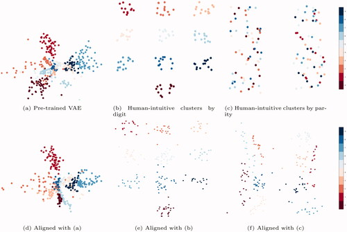
Another, more intuitive, example of latent space alignment is depicted in Figure 1. The top row demonstrates how different agents (e.g., humans or pre-trained models) may represent data in different ways. In this case, the 2 D dots are encodings of images from the MNIST digit dataset – images of hand-written digits. In the leftmost diagram, a variational autoencoder (VAE) created clusters of encodings by digit; humans might similarly create clusters by digit (middle) or parity (right). The bottom row of Figure 1 shows the latent spaces learned by agents trained by a technique we developed to align with the latent spaces in the top row. Because different agents may use different representation formats, or the same agent may use different representations for different tasks (e.g., clustering by parity vs. digit depending upon what one cares about), it is important that techniques for solving the latent space alignment problem work for many different latent spaces.

Figure 1. (a) When encoding images of hand-written digits, a standard VAE with a 2 D latent space creates clusters by digit. More intuitive designs may create other patterns of clusters by digit (b) or parity (c), depending upon the task. In all cases, we trained agents to align with their partners (d–f). (a) Pre-trained VAE. (b) Human-intuitive clusters by digit. (c) Human-intuitive clusters by parity. (d) Aligned with (a). (e) Aligned with (b). (f) Aligned with (c).

In this article, we focus on techniques that enable agents to align their latent spaces with their partner’s. Prior art in interpretability research suggests ways in which agents may align with human intuition, but such techniques are limited to enabling good human-machine partnerships instead of also supporting machine-machine partnerships (Li et al., 2018). Recent techniques developed in social convention literature supports the flexibility of partnering with arbitrary autonomous agents but was not evaluated in the context of human partners (Lerer & Peysakhovich, 2018). We extended social convention work and developed a new technique, Adversarially Guided Self-Play (ASP), that enabled efficient latent space alignment with human or machine partners. The bottom row of Figure 1 shows the latent spaces learned by agents trained using ASP to align with partners’ latent space, represented in the top row; despite using as few as 8 examples of images and representations from their partners, our agents aligned their 2 D latent spaces with their partners’. Experiments in which our agents partnered with other machines or with humans demonstrated that our technique produced better-aligned agents than the state of the art.

Our contributions are thus three-fold. First, we defined the problem of latent space alignment and proposed two metrics for measuring alignment. Second, we designed and implemented a new technique, ASP, for efficiently solving the latent space alignment problem. Third, we demonstrated the benefit of ASP compared to existing techniques, as measured in a series of experiments in which agents partnered with other machines or humans.

2. Latent space alignment problem

Here, we define the latent space alignment problem as a learning problem that encourages commonality of representation functions among agents on a team. First, we introduce a set of assumptions about team membership that simplify the problem definition. Second, we create a semantic measure of latent space alignment that computes the average similarity between representations that different agents generate for the same input. The latent space alignment problem is defined a finding parameters of an agent that minimizes this semantic measure. Finally, given that the semantic measure is not computable in all settings, we define an additional metric—pragmatic alignment—that may be calculated more broadly and correlates closely with semantic alignment.

2.1. Problem scope

As motivated in the introduction, we wish to create agents that operate well in teams comprising heterogeneous agents by training new agents to use the same representation scheme as their teammates. For the sake of simplicity, we limit our attention to two-member teams, meaning that a new agent must partner well with a single other agent. (Generalizing to larger teams is feasible, and related research has found regularizing effects in training with many partners, but these larger group dynamics are outside the scope of this work (Hernandez-Leal et al., 2019).) We limit our attention to classification tasks with an intermediate representation generated during computation. Concretely, this means that each of the two partners in a team employs at least two functions: an encoder, e, that maps input x to an encoding z ($e:R^X\to R^Z$) and a classifier, c, that maps an encoding z to a probability distribution over Y mutually exclusive categories. The classification of an input by an agent is calculated as the argmax of the composition of these two functions: $\widehat{y}=\arg \max (c(e(x))).$

For two-member teams, the problem of latent space alignment corresponds to the notion of encodings produced by each agent being similar in some way. Recall that in our motivating example of a firefighter and a local expert communicating via a map about a burning building, it was important for them to understand the map in the same way: if they disagreed about which direction corresponded to north, the map would be useless. Analogously, our agents must create representations from inputs, and both team members must do so similarly. We define this notion more rigorously in the next section.

2.2. Semantic measure of latent space alignment

We first construct a semantic measure of latent space alignment that measures the distance, on average, between encodings of the same input by two different agents. We borrow the word “semantic” from linguistics literature that defines semantics as “literal, decontectualized meaning” (Frawley, 2013). Thus, if encodings are thought of as the “meanings” of inputs, a semantic measure of latent space alignment should reflect how close the outputs of two agents’ encodings functions are.

Mathematically, we define a function $a_S(A,B,X)$ that, given two agents A and B and a dataset of inputs X, returns the real-valued semantic latent space alignment of the two agents. The formulas for calculating $a_S(A,B,X)$ are written below, with e_A and e_B denoting the encoding functions of agents A and B, respectively. (1) $$\begin{array}{cc}{a}_S(A,B,X)\hfill & =-\frac{1}{Z\left|X\right|}\sum _{x\in X}{(e_A(x)-e_B(x))}^2\hfill \end{array}$$(1) (2) $$\begin{array}{cc}Z\hfill & =\frac{1}{|X{|}^2}\sum _{i\in [1,\dots ,|X\left|\right]}\sum _{j\in [1,\dots ,|X\left|\right]}{(e_A(x_i)-e_B(x_j))}^2\hfill \end{array}$$(2)

Equation (1)(1) $$\begin{array}{cc}{a}_S(A,B,X)\hfill & =-\frac{1}{Z\left|X\right|}\sum _{x\in X}{(e_A(x)-e_B(x))}^2\hfill \end{array}$$(1) calculates the semantic alignment of agents A and B by measuring the negative of the mean squared error (MSE) of the encodings generated by the encoding functions of the agents. A factor of $\frac{1}{Z},$ with Z defined in Equation (2)(2) $$\begin{array}{cc}Z\hfill & =\frac{1}{|X{|}^2}\sum _{i\in [1,\dots ,|X\left|\right]}\sum _{j\in [1,\dots ,|X\left|\right]}{(e_A(x_i)-e_B(x_j))}^2\hfill \end{array}$$(2) , is included to normalize the alignment quantity by the MSE of encodings from all pairs of inputs, thus cancelling out the penalty agents with large numerical values for encodings would otherwise face. Together, these two equations measure how far apart the encodings generated by different agents are for the same input, compared to the average distance for randomly chosen inputs. We set a_S as the negative of the (normalized) MSE in order to have lower scores correspond to worse-aligned agents, with a maximum possible value of 0 if the two encoding functions are identical.

Given this definition of semantic alignment, we formalize the latent space alignment problem as the learning problem that follows: (3) $$\begin{array}{cc}{A}^{*}\hfill & =\underset{A\in A}{\mathrm{arg\hspace{0.17em}max}}{a}_S(A,B,X)\hfill \end{array}$$(3)

In other words, solving the latent space alignment problem produces the optimal agent ($A^{*}$) from a class of possible agents ($A,$ e.g., a set of neural nets of a given architecture) that maximizes the semantic alignment for a fixed partner (B) and dataset (X).

Although we have formalized the latent space alignment problem as a minimization problem, in some settings, one cannot directly compute the value being minimized. Crucially, the semantic measure of alignment requires access to numerical values of encodings, which may not always be possible. For example, when assessing the latent space alignment between an agent and a human, it is not obvious how one would convert a human’s encoding of an input into the form required by a_s. Thus, our semantic measure of latent space alignment provides a formal definition of the latent space alignment problem and is useful when applicable, but only applicable in some situations.

2.3. Pragmatic measure of latent space alignment

To complement the effective but limited semantic measure of latent space alignment, we introduced a pragmatic metric that, while not directly measuring distances in the latent space, is more broadly applicable. Within linguistics, pragmatics “involves the selection of the contextually relevant meaning, not the determination of what counts as the meaning itself” (Frawley, 2013). Thus, rather than compare encodings (loosely equivalent to meaning), we measured the effect of encodings in the context of classification tasks. We did so by measuring task performance when one agent’s encoder and the other agent’s classifier were composed, as shown in Equation (4)(4) $$a_P(A,B,X,Y)=\frac{1}{2\left|X\right|}\sum _{(x,y)\in (X,Y)}[1_{y=c_a(e_b(x))}+1_{y=c_b(e_a(x))}]$$(4) . (4) $$a_P(A,B,X,Y)=\frac{1}{2\left|X\right|}\sum _{(x,y)\in (X,Y)}[1_{y=c_a(e_b(x))}+1_{y=c_b(e_a(x))}]$$(4)

Given the above equation, the pragmatic alignment of agents A and B using a dataset of paired inputs and outputs, (X, Y), $a_P(A,B,X,Y),$ is the mean classification accuracy when the encoder of A (e_A) is composed with the classifier of B (c_B) and the encoder of B (e_B) is composed with the classifier of A (c_A). This measure of alignment may intuitively be thought of as measuring how well information may be passed among agents’ latent spaces; if the classification accuracy is high, the two agents must be able to “understand” each other to some extent, which corresponds to a high value of a_P.

Compared to the semantic measure of alignment, this pragmatic measure is less discerning but more broadly applicable. On the one hand, using a_P may mask subtle differences in encoding functions between agents, as long as the agents remain able to make correct classification decisions. On the other hand, a_P mitigates the limits introduced by a_S in directly measuring distances in the encoding space of agents; one can measure task performance with humans as partners without ever directly measuring a human’s internal representations. Lastly, note that, assuming individually-optimal agents A and B, pragmatic alignment is maximized when semantic alignment is maximized as well; in addition, we confirmed in experiments that the two measures are correlated.

3. Background

This article applied two techniques from prior art to the context of latent space alignment. These techniques were used as baselines against which to compare our proposed technique and are reviewed in detail in this section; a broader review of related literature is included in Section 14.

3.1. Observationally Augmented Self-Play

Observationally Augmented Self-Play (OSP) is a data-efficient technique for learning social conventions (Lerer & Peysakhovich, 2018). Framed in the context of multi-agent games, the authors set out to train new agents to learn a fixed agent’s policy such that, when the new agent and fixed agent worked together, they achieved a high reward in the game. A simple example of this sort of behavior was a new agent learning to drive on the right or left side of roads in a simulated grid, choosing a side in order to diminish the likelihood of crashing with the other agent.

In training a new agent, OSP assumes access to an environment with a reward function and a small amount of “paired” data characterizing the fixed agent’s behavior. These paired data take the form of state-action pairs of states from the environment and subsequent actions that the fixed agent’s policy produced. The key insight of OSP is that combining self-play in the environment with supervised training of paired data guides a new agent to learn to the fixed agent’s policy. Intuitively, this occurs because self-play encourages the new agent to adopt one of potentially many optimal policies, while the supervised data breaks ties between optima to favor the right policy. In the driving example, this corresponds to optimal driving strategies resulting in all agents driving on the right or left side of the road, while paired data specify that in some specific instances, the fixed agent drove on one particular side of the road, breaking the tie.

While OSP was developed in the context of multi-agent RL games, we claim that it may equally well be applied to the problem of latent space alignment. In this context, the social convention that must be learned is the meaning of representations. Indeed, the encoding function e and classifying function c may be thought of as independent agents that must agree upon the interpretation of representations. The environment reward, which drove the new agent’s policy to optimality in OSP’s formulation, may be replaced by supervised classification loss to the same effect. Similarly, paired state-action data may be replaced by inputs and corresponding representations.

3.2. The Prototype Case Network

In addition to OSP, we also studied Prototype Case Networks (PCNs) within the context of latent space alignment (Li et al., 2018). Originally, PCNs were introduced as a technique for building interpretable neural network classifiers. The intuition behind the networks was to learn meaningful prototypes and simple classification rules, thus making it easier for humans to understand how a PCN works.

Concretely, a PCN is a neural net composed of four parts: an encoder, a decoder, latent prototypes, and a linear classifier. The encoder and decoder serve the traditional roles of mapping high dimensional inputs to low-dimensional latent representations and back (Kingma & Welling, 2014). The latent prototypes are a set of k (specified by the researcher) trainable points in the latent space. Lastly, a linear layer generates classification distributions of an encoding by taking the softmax of a weighted sum of l2 distances from an encoding to each prototype in the latent space, with the weights determined by the linear layer. Thus, inputs are classified by passing them through the encoder, calculating the distance to each prototype, and passing those distances through the linear layer. In addition, prototypes may be visualized by passing the latent prototypes through the decoder. The whole network may be trained end-to-end by a loss function that encourages good reconstructions, high classification accuracy, and tight clustering between prototypes and encodings of inputs. For further details, we encourage readers to examine the original paper describing PCNs (Li et al., 2018).

The results presented with the development of PCN are promising and hint at human-aligned latent spaces. In classifying digits from MNIST images, for example, encodings formed clusters around prototypical digits. Thus, although the latent spaces learned by PCNs may not align with other machines’ representations, it appears plausible that the inductive biases of the architecture and training terms are sufficient to match humans’ representations.

4. Technical approach

In addition to the two techniques discussed above, we developed a new technique for latent space alignment that improves upon the data efficiency of OSP. We maintained the underlying notion of framing latent space alignment as learning a social convention, because such a framing allows for adopting any other agent’s representation, not just a human’s. However, we introduced an adversarial training technique to shape the latent space, which constrained the set of learned representations and therefore improved performance for the same amount of paired training data. In this section, we have detailed the technique we developed, Adversarially Guided Self-Play (ASP), and analyzed the resulting benefits.

4.1. Adversarial shaping of latent spaces

In developing ASP, we supplemented the technique proposed in OSP with adversarial training to shape the learned latent space. Thus, as in OSP, we required access to a classification dataset ((X, Y) pairs for supervised learning of the task) and a set of paired data, P, comprising inputs and associated representations, (X, Z).

In addition to those two datasets, ASP required the addition of a third dataset of representations without associated inputs. This unpaired dataset, Z, described the distribution of representations that the partner generated. Such data are often easier to gather than paired data: for example, if language is thought of as a representation for ideas, it is much easier to gather a corpus of English sentences than a set of ideas and associated language.

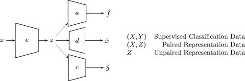
The architecture of the agents we trained is depicted in Figure 2. The encoding and classification functions detailed in our problem formulation are instantiated as neural networks, e and c. In addition, a decoder, d, reconstructs inputs from representations. Lastly, an adversary network, a, predicts whether an encoding is fake (generated from the encoder) or real (from a dataset of unpaired encodings Z).

Figure 2. An encoder maps input, x, into representation, z. From z, an adversary, a, predicts whether the representation was fake or real, a classifier, c, estimates a classification $\widehat{y},$ and decoder, d, creates a reconstruction $\widehat{x}$ of the original input. Classification, paired, and unpaired data may be used in training. (X, Y) Supervised Classification Data. (X, Z) Paired Representation Data. (Z) Unpaired Representation Data.

The training loss for e, d, and c is composed of four weighted terms (with positive, real-valued weights of terms denoted by λs), representing the four simultaneous objectives of high classification accuracy, high-quality reconstructions, matching the paired representation data, and fooling the adversary. The adversary, conversely, is trained to distinguish between fake encodings and those drawn from the dataset, Z, of unpaired encodings. The loss functions are shown in Equations (5)(5) $$\begin{array}{cc}\mathit{loss}\hfill & ={\lambda }_1\frac{1}{|(X,Y)|}\sum _{(x,y)\in (X,Y)}{1}_{y\hspace{0.17em}=\hspace{0.17em}\arg \max c(e(x))}\hspace{0.17em}\text{log}\hspace{0.17em}c(e(x))\hfill \\ \hfill & +{\lambda }_2\frac{1}{\left|X\right|}\sum _{x\in (X,Z)}(x-d(e(x)){)}^2\hfill \\ \hfill & +{\lambda }_3\frac{1}{|(X,Z)|}\sum _{(x,z)\in (X,Z)}(z-e(x){)}^2\hfill \\ \hfill & -{\lambda }_4\frac{1}{\left|X\right|}\sum _{x\in X}\hspace{0.17em}\text{log}\hspace{0.17em}a(e(x))\hfill \end{array}$$(5) and (6)(6) $$\begin{array}{cc}\mathit{los}{s}_{\mathit{adv}}\hfill & =\frac{1}{\left|X\right|}\sum _{x\in X}\hspace{0.17em}\text{log}\hspace{0.17em}a(e(x))+\frac{1}{\left|Z\right|}\sum _{z\in Z}\hspace{0.17em}\text{log}\hspace{0.17em}(1-a(z))\hfill \end{array}$$(6) ; note the switched sign for the adversarial training term that encourages e to fool the adversary. (5) $$\begin{array}{cc}\mathit{loss}\hfill & ={\lambda }_1\frac{1}{|(X,Y)|}\sum _{(x,y)\in (X,Y)}{1}_{y\hspace{0.17em}=\hspace{0.17em}\arg \max c(e(x))}\hspace{0.17em}\text{log}\hspace{0.17em}c(e(x))\hfill \\ \hfill & +{\lambda }_2\frac{1}{\left|X\right|}\sum _{x\in (X,Z)}(x-d(e(x)){)}^2\hfill \\ \hfill & +{\lambda }_3\frac{1}{|(X,Z)|}\sum _{(x,z)\in (X,Z)}(z-e(x){)}^2\hfill \\ \hfill & -{\lambda }_4\frac{1}{\left|X\right|}\sum _{x\in X}\hspace{0.17em}\text{log}\hspace{0.17em}a(e(x))\hfill \end{array}$$(5) (6) $$\begin{array}{cc}\mathit{los}{s}_{\mathit{adv}}\hfill & =\frac{1}{\left|X\right|}\sum _{x\in X}\hspace{0.17em}\text{log}\hspace{0.17em}a(e(x))+\frac{1}{\left|Z\right|}\sum _{z\in Z}\hspace{0.17em}\text{log}\hspace{0.17em}(1-a(z))\hfill \end{array}$$(6)

Although these equations have many terms, they reflect the standard training losses used often in classification tasks (the categorical cross entropy term), autoencoders (the mean squared error of reconstructions and inputs), regression tasks (the term for paired inputs and representations), or adversarial training (the adversary terms). Having written the loss function, training the model consisted of finding the parameters of e, a, d, and c to minimize the loss. We used Keras with a tensorflow backend to instantiate and train our models; code and trained models will be provided online upon paper acceptance (Chollet et al., 2015).

4.2. Analysis of adversarial pruning

In developing ASP, we hypothesized that using an adversary in training would enable agents to learn well-aligned latent spaces more efficiently. In this section, we confirmed this intuition by analyzing the effects of ASP in reducing the number of possible learned encoding functions. We focused on the degree of pruning: how many functions were ruled out by a well-trained adversary. Both intuitively and formally, using an adversary constrained the set of possible learned latent spaces, leading to more efficient learning of the correct alignment.

4.2.1. Intuition of adversarial pruning

The intuition behind the advantages conferred by adversarial training is simple: using an adversary forced the learned encoding function to conform to a desired distribution of outputs, which reduced the number of possible functions that could be learned, leading to better-aligned latent spaces.

Consider the example of the firefighter and expert drawing on a map. Recall that the expert must communicate a safe path for the firefighter to follow through a burning building. If the expert were to draw a line that crossed through walls or was implausible in some other way, the firefighter could immediately state that, regardless of what path the expert was actually trying to convey, the firefighter cannot understand the drawing. This corresponds to adversarial training: paths that go through walls do not fall within the distribution of paths the firefighter is willing to take. Only after the expert begins to draw realistic paths does it make sense to consider other aspects of communication, such as the orientation of the map.

4.2.2. Discrete case analysis

Here, we mathematically examine the benefits of adversarial pruning and confirm the intuition from earlier. Consider a discrete representation problem with $X=\left|\mathit{X}\right|$ discrete inputs, Z possible discrete encodings, and a pre-trained encoding function e that maps from inputs to encodings. We seek to learn a function, f, that best approximates e, but in the absence of further information, there exist Z^X possible functions, as each input could map to any encoding.

When training with ASP, we have access to a dataset of unpaired representations, which describes the distribution that e produces: $p_i=\sum _{x\in \mathit{X}s.t.e(x)=z_i}P(x).$ Thus, we may constrain f to belong to the set of all functions for which subsets of the inputs with probabilities that sum to p_i map to representation z_i. Calculating the size of this set of functions—functions that are constrained to match e in distribution—is a combinatorics problem: there are $\left(\begin{array}{c}X\\ p_{0}X,p_{1}X,\dots ,p_{Z-1}X\end{array}\right)$ such functions. A small value implies a greater advantage from adversarial pruning.

The fact that the number of such functions is the multinomial coefficient implies that the advantage depends upon the distribution described by the p_i’s. We therefore analyze the advantage conferred by ASP in the worst case: the uniform distribution. Our analysis measures the log ratio (lr) of adversarially allowed encoding functions to all possible functions. (7) $$\begin{array}{cc}lr\hfill & =\hspace{0.17em}\text{ln}\hspace{0.17em}\left(\frac{\left(\begin{array}{c}X\\ p_{0}X,\dots ,p_{Z-1}X\end{array}\right)}{Z^X}\right)\hfill \end{array}$$(7) (8) $$\begin{array}{cc}\hfill & =\hspace{0.17em}\text{ln}\hspace{0.17em}\left(\begin{array}{c}X\\ p_{0}X,p_{1}X,\dots ,p_{Z-1}X\end{array}\right)-\hspace{0.17em}\text{ln}\hspace{0.17em}(Z^X)\hfill \end{array}$$(8) (9) $$\begin{array}{cc}\hfill & =\hspace{0.17em}\text{ln}\hspace{0.17em}\left(\frac{X!}{{(\frac{X}{Z}!)}^Z}\right)-X\hspace{0.17em}\text{ln}\hspace{0.17em}(Z)\hfill \end{array}$$(9) (10) $$\begin{array}{cc}\hfill & =\hspace{0.17em}\text{ln}\hspace{0.17em}(X!)-Z\hspace{0.17em}\text{ln}\hspace{0.17em}\left(\frac{X}{Z}!\right)-X\hspace{0.17em}\text{ln}\hspace{0.17em}(Z)\hfill \end{array}$$(10) (11) $$\begin{array}{cc}\hfill & =X\hspace{0.17em}\text{ln}\hspace{0.17em}(X)-X+O(\hspace{0.17em}\text{ln}\hspace{0.17em}(X))-X\hspace{0.17em}\text{ln}\hspace{0.17em}\left(\frac{X}{Z}\right)+X-ZO\left(\hspace{0.17em}\text{ln}\hspace{0.17em}\left(\frac{X}{Z}\right)\right)-X\hspace{0.17em}\text{ln}\hspace{0.17em}(Z)\hfill \end{array}$$(11) (12) $$\begin{array}{cc}\hfill & =O\left(\hspace{0.17em}\text{ln}\hspace{0.17em}(X)-Z\hspace{0.17em}\text{ln}\hspace{0.17em}\left(\frac{X}{Z}\right)\right)\hfill \end{array}$$(12)

The steps from Equations (7)–(10) follow from the repeated application of log rules, the definitions of combinatorial terms, and the assumption of the worst-case uniform probability distribution. Equation (11)(11) $$\begin{array}{cc}\hfill & =X\hspace{0.17em}\text{ln}\hspace{0.17em}(X)-X+O(\hspace{0.17em}\text{ln}\hspace{0.17em}(X))-X\hspace{0.17em}\text{ln}\hspace{0.17em}\left(\frac{X}{Z}\right)+X-ZO\left(\hspace{0.17em}\text{ln}\hspace{0.17em}\left(\frac{X}{Z}\right)\right)-X\hspace{0.17em}\text{ln}\hspace{0.17em}(Z)\hfill \end{array}$$(11) comes from the application of Stirling’s approximation, which remains accurate even for small numbers but introduces big-O notation. Finally, Equation (12)(12) $$\begin{array}{cc}\hfill & =O\left(\hspace{0.17em}\text{ln}\hspace{0.17em}(X)-Z\hspace{0.17em}\text{ln}\hspace{0.17em}\left(\frac{X}{Z}\right)\right)\hfill \end{array}$$(12) is derived from subsequent cancellation of terms and more application of log rules.

The final expression for the log ratio shows how the degree of pruning varies as the number of inputs and encodings changes. As the number of inputs increases, the log ratio decreases, meaning the adversary prunes a greater proportion of functions. Conversely, as the number of representation grows (up to the limit of X = Z, corresponding to a unique representation per input), the log ratio increases. Thus, ASP confers its greatest advantage when the number of encodings is small relative to the number of inputs, which, given that the goal of encoding functions is often to generate compact representations, should often be the case.

Although the above analysis was conducted for functions mapping from a discrete set of inputs to a discrete set of representations, the same intuition applies to the continuous case. Adversarial pruning fixes the learned function to output the correct distribution in the representation space, but given the continuous nature of the function domains and ranges, we are unable to calculate standard ratios, as was done in the discrete case.

5. Experiment overview

To complement the mathematical analysis in the previous section, we designed a series of experiments to measure the ability of different techniques to train agents with latent spaces aligned with a partner’s. Each experiment shed light on a different aspect of either the latent space alignment problem broadly, or on the performance of different training techniques. Table 1 summarizes each of the experiments.

Table 1. A high-level summary of the experiments detailed in the remainder of this paper.

Section	Experiment	Findings
7	Semantic measure of individualized robot-robot alignment	New agents aligned with pre-trained agents; performance was measured via semantic metric.
8	Pragmatic measure of individualized robot-robot alignment	Using the pragmatic metric of alignment confirmed trends from semantic measure.
9	Varied latent space dimensionality and amount of paired data for robot-robot alignment	Changing the dimensionality of agents’ latent spaces and the amount of paired data affected ASP’s advantage over OSP.
10	Human-robot pragmatic alignments	Humans were able to select or interpret encodings for high pragmatic alignment with agents.
11	Human participants created encodings for robots by drawing	Humans were able to create encodings from scratch that caused ASP-trained agents to correctly classify inputs.
12	Human participants predicted robot successes of failures	Humans were able to appropriately calibrate their trust of machines, especially using ASP and useful latent designs.

The first half of the experiments measured the ability of agents to align with other agents; the second half studied how well agents that had been trained to align with human-designed latent spaces could partner with humans.

These experiments explored different aspects of latent space alignment. First, we measured the ability of agents to align with other, pre-trained, agents. Within these robot-robot teams, we recorded both the pragmatic and semantic metrics of latent space alignment; both metrics indicated that ASP outperformed OSP, which indicated that the pragmatic measure of alignment is a reasonable proxy for semantic alignment. Given the flexibility of robot-robot teams, we explored how the relative benefits of ASP over OSP varied as a function of the model architectures. Second, we conducted human-participant studies to evaluate the extent to which agents could align with human representations. In these experiments, we trained agents to align with latent spaces designed by the research team. Measuring semantic alignment was impossible with humans, but the pragmatic measure revealed that humans were able to form effective teams with ASP-trained agents. Finally, human participant studies established that the same agents that resulted in high human-agent latent space alignment also supported well-calibrated participant trust in agents.

The following sections present each experiment with associated results and analysis. First, we review preliminary information on experiment design that many of our experiments had in common: the types of data and associated tasks that we used to analyze team performance. Subsequent sections explain each experiment in more detail, including metrics and analysis.

6. Experiment preliminaries

In designing the evaluations for this work, we created experimental domains to examine particular aspects of the latent space alignment problem. First, we used two broad sets of data (the MNIST digit dataset and a dataset of recorded human motion trajectories) to allow us to draw conclusions beyond one specific domain. Second, for each dataset, we devised two classification tasks. Separating the task from the input data was important in our analysis of the utility of latent spaces for particular tasks. In some of our experiments, including all human-subject studies, we trained models to align with human-designed latent spaces. We hypothesized that certain designs would be most useful for certain tasks; creating two tasks per dataset enabled us to measure the relationship between latent space design and changes in task performance, holding the input data constant. In this section, we described the data, tasks, and latent space designs employed in all our experiments.

Our first dataset was the MNIST digit image dataset, used for two tasks. In the first task, parity prediction, machines were trained to reconstruct MNIST images and predict the parity of the digit (even or odd) with a softmax output over 2 neurons at the end of the classifier. In the second task, digit prediction, machines were likewise trained via reconstruction loss of the images, but the output of the classifier was a softmax over 10 neurons, corresponding to each digit. In both cases, we allowed PCNs to use 10 prototypes.

Our second dataset was a series of trajectories of humans placing bolts on a table in a lab setting; as with the MNIST data, these trajectories were used for two tasks. First, for intersection prediction, models learned to classify whether a pair of trajectories crossed. Second, for target prediction, models were trained to predict the location a human was reaching toward given their prior motion. (Note that, intuitively, the intersection and target prediction tasks correspond in some way to the firefighter in the example seeking a path and a destination in a burning building.) The data within the trajectory dataset tracked participants’ motion during an assembly task involving the placement of 8 bolts in any order. A motion-capture system recorded the 3 D location of the participants’ gloved hand at 50 Hz.

After recording a full run, we hand-labeled the motion data to indicate which of 8 bolt locations the participant reached for next. (If, for example, a participant had just placed a bolt in location 0 and was next going to place a bolt in location 7, every point until the participant reached location 7 was labeled as “7.”) The labeled full runs were divided into 1-s trajectories by stepping through each run at 0.2-s increments (i.e., a full run would generate a trajectories for the motion from time 0 to 1 s, from 0.2 to 1.2 s, from 0.4 to 1.4 s, etc.). Figure 3(a) depicts an example of a complete run, segmented into 1-s trajectories. Our models accepted the 1-s trajectories as flattened vectors; that is, 150 points fed into a fully connected layer, representing the 50 Hz times 3 dimensions.

Figure 3. Human motion data (a) was used for target prediction and intersection classification (b). (a) Two views of the same full run plotted within 3D axes normalized by the full range of all participants’ motion. Participants picked up bolts at the bottom of the plot and placed them in one of eight locations at the top. The colored segments each represent 1 second of motion within the run. (b) The model for classifying intersections used duplicate encoders and decoders for trajectories, and a single predictor net.

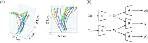
The intersection prediction task was to classify, given two 1-s trajectories, whether the trajectories overlapped in the x – z plane (corresponding to a person reaching over another person’s hand while moving toward a bolt). This type of task is important: we would like machines to be able to determine if trajectories are a safe distance apart from one another. Rather than building a single encoder that would take in both trajectories and would therefore have to compute a single representation for them jointly, we modified our model design to create two instances of the encoder net and two of the decoder net that each handled a single trajectory separately. (For ASP, we likewise created two instances of an adversary net, each consuming only a single representation.) Only the predictor net consumed the latent representations of both trajectories to make the overlapping classification decision; in other words, the learned representations only modeled a single trajectory each. This design decision was also critical to the PCN implementation, which, while learning 64 prototypes (inspired by the 8 bolts each for the first and second trajectories), would have had to create prototypical encodings for trajectory pairs, whereas with our design, prototypes were decomposable into prototypes for each separate trajectory. Figure 3(b) shows the basic architecture of the intersection classifier.

The target prediction task was to predict, given a 1-s trajectory, which bolt location the participant was reaching for next. This task is non-trivial for several reasons: participants were allowed to choose bolt locations in arbitrary orders during data collection, human motion rarely obeys simple heuristics like minimizing straight-line distance, and some 1-s trajectories were not very informative (e.g., if a participant had just placed a bolt at location 0 and was reaching to pick up a new bolt, it was unclear where that new bolt may go). The PCN was allowed to learn 8 prototypes, inspired by the 8 target locations. The models predicted the target location via an 8-neuron softmax layer at the end of the classifier.

These four tasks—parity, digit, intersection, and target—were used throughout the experiments listed in the rest of this article. Those experiments changed many factors, such as whether agents were paired with other agents or with humans, but the underlying structure of each experiment was the same: agents were trained in a classification task and we measured how well the latent spaces those agents learned were aligned with their partner’s representations.

In our human-participant experiments, we wished to create agents that aligned in some sense with the representations humans used. Directly measuring humans’ encodings of inputs was impossible, so we instead created latent space designs to train new agents to align with latent spaces that had been designed by the research team. These designs, shown in Figure 4, were hand-crafted rules that mapped inputs to points in a latent space. For example, we created a 2 D latent space that mapped MNIST images to points in a 2 D plane, clustering points by digit in a dialpad-like pattern. In training, these designs were used to generate the paired data required by OSP and ASP and the unpaired data additionally required by ASP.

Figure 4. Latent space designs for the MNIST (a) and trajectory (b) domains. (a) Designs for latent spaces for the MNIST tasks created clusters by parity (left) or in a dialpad pattern by digit (right). (b) Trajectories (left) were mapped to 2D representations based on target bolt location (middle) or converted to a sketch (right). Examples of learned latent spaces conforming to these designs are included in Appendix A.

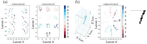
For both of the MNIST and trajectory-related tasks, we created two latent space designs. For MNIST, both designs operated in 2 D latent spaces, creating 10 clusters by digit in a dialpad-like structure, or in 2 clusters by parity. For the trajectory data, one design created a ray-like structure of encodings in 2 D, clustered by target bolt. We also developed a more complex design in the form of “sketches,” or 16 × 16 pixel drawings of trajectories collapsed along the y axis. In other words, sketches depicted the coarsely pixelated occupancy of the points a person reached over in the course of a given trajectory, in a manner similar to how a human might draw quickly on paper. The latent designs in the bolt domain experiments were inspired by the “X” and sketches employed in the firefighting example.

Just as we introduced two tasks per input data (i.e., parity and digit for MNIST, and intersection and target for trajectories), we used two latent designs in order to separate the effect of a particular design from other aspects of our experiments. Specifically, we hypothesized that some latent designs would enable high performance for some tasks, but lower performance in others. For example, creating clusters by the parity of an MNIST figure would likely be useful in the parity task but less useful in the digit task. Lastly, while experimental results indicated that the designs chosen by the research team indeed did support good human-robot interaction, it is worth noting that the designs used in these experiments could certainly be improved.

7. Individualized robot-robot semantic alignment

In our first experiment, we investigated the extent to which different training techniques allowed new models to learn an existing model’s latent space. For example, if a model had been trained end-to-end to predict a digit from an MNIST image, with no supervision to guide its learned representation, could a new model align with first model’s latent space?

For each of the four tasks, we trained 10 predictive autoencoders (PAEs), each using a 2-dimensional latent space. (PAEs were simple encoders, decoders, and classifiers; one may equivalently think of them as OSP- or ASP-trained models without the representation training losses.) We then trained 10 new models, using both ASP and OSP, to do the same task, but this time we generated paired and unpaired representation data by querying the pre-trained PAEs. Given that interpretability-inspired models like PCNs were designed neither to partner with machines nor accept data to guide learned latent representations, we did not include PCNs in this experiment. Teams were formed by partnering the new models with their corresponding PAEs.

In evaluating the models trained by each technique, we calculated the semantic measure of latent space alignment between the ith ASP- or OSP-trained model, A_i, and the ith PAE model, PAE_i, as $a_S(A_i,PA{E}_i,X).$ Recall that a_S measured the negative mean squared error of encodings generated by two different agents. We plotted the median and quartile semantic measures of latent space alignment for each task, normalized by the median value of the alignment for OSP-trained models for that task, in Figure 5.

Figure 5. Median (and quartile) MSE of encodings generated by models and their trained partners, normalized by MSE of OSP for that task. For the same task and amount of paired data (in parentheses), models trained with ASP generated significantly closer encodings to their partner’s (p < 0.05).

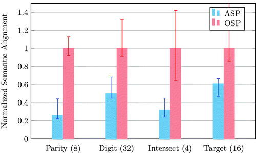
The results demonstrated that the agents trained with ASP were consistently better-aligned with their PAE partners than the OSP-trained models. The lower values for ASP show that compared to OSP, ASP-trained models routinely generated encodings that were closer to the encodings the PAE partners generated. Furthermore, because both the ASP- and OSP-trained models were trained from the same original 10 PAE models, we may conclude that the difference in training technique was the cause of the better alignment instead of, for example, differences among the PAE partners. Thus, as measured by the semantic measure of latent space alignment, ASP outperformed OSP.

8. Individualized robot-robot pragmatic alignment

To complement the analysis of ASP and OSP by comparing values of semantic latent space alignment, we also recorded the pragmatic measures of latent space alignment. That is, using the same models (A_i and PAE_i) that had been trained for the experiment in the previous section, we recorded $a_P(A_i,PA{E}_i,X,Y)$ for each of the 4 tasks. Although the pragmatic and semantic measures of latent space alignment differ, if they are faithful proxies to an underlying notion of alignment, the trends recorded in the previous section should be reflected in measures of pragmatic alignment as well. The results of measuring pragmatic alignment for all 4 tasks are plotted in Figure 6.

Figure 6. Median (and quartile) classification accuracy for mixed teams with models trained on their partner’s latent space. For the same amount of paired data on a given task, noted in parentheses, ASP outperformed OSP (p < 0.05).

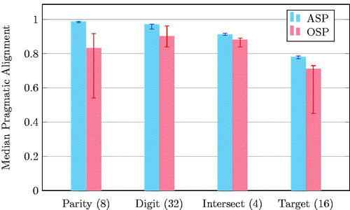
As expected, the results confirmed that models trained by ASP resulted in higher pragmatic alignment scores than OSP-trained models. Recall that the pragmatic metric of latent space alignment measured classification accuracy, so the higher bars for ASP indicate that it consistently resulted in better team performance than OSP.

These results are important for two reasons. First, the results themselves speak to the fact that, for the same amount of paired data as OSP, ASP yielded better-aligned models. Second, the results confirm that the trend of better alignment, as measured by our semantic measure of alignment, was reflected in our measure of pragmatic alignment as well. This indicates that pragmatic alignment is a good proxy for semantic alignment and offers hope that, when measuring semantic alignment is not possible, we may still be able to use the pragmatic measure. Lastly, it is worth noting that the magnitude of the differences between ASP and OSP was relatively smaller when measured by pragmatic alignment. This corresponds with the notion that minor mis-alignments in latent spaces may be masked by the coarser evaluation metric of classification accuracy; thus, if anything, the pragmatic measure of latent space alignment likely underestimates differences among training techniques.

9. Changes in latent space dimensionality and amount of paired data

The two previous experiments demonstrated that, as measured by both semantic and pragmatic metrics, ASP resulted in better-aligned models than OSP. In earlier theoretical analysis of ASP, we derived that the advantage of ASP over OSP is not constant: rather, it depends upon the relative sizes of input and representation spaces. Likewise, the analysis indicated that rotational ambiguities could not be solved by ASP without paired data, so the benefit of ASP over OSP likely varies as a function of the amount of paired data used in training. In this section, therefore, we analyzed the extent to which ASP-trained models outperformed OSP-trained models within the MNIST domain, as the dimensionality of the latent space and the number of paired data changed.

Our results were plotted in Figure 7. We used a pragmatic measure of latent space alignment by measuring task performance of mixed teams; however, rather than measure classification accuracy, we measured the image reconstruction loss as the MSE between the input image and decoded image. (We used reconstruction loss simply because it revealed more fine-grained differences in alignment than the cruder, digit-based alignment necessary for high classification accuracy.) For each training technique, latent dimensionality, and number of training examples, we first trained 10 PAE’s on the MNIST data and then trained new models using ASP or OSP to complement the PAE. Median and quartile mixed-team reconstruction MSE’s are plotted.

Figure 7. For a fixed number of paired examples (32), ASP generated better MNIST reconstructions than OSP for varying latent dimensionality (left). For a fixed latent dimension (32), ASP outperformed OSP for varying numbers of paired examples (right).

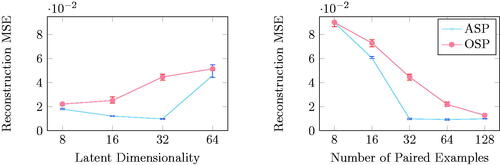
The results supported our conclusions from previous experiments. First, for the same latent dimensionality and amount of paired data, ASP-trained models consistently outperformed OSP-trained models. Second, the leftmost plot sheds light on the utility of ASP in high-dimensional latent spaces. Using a higher-dimensional latent space enabled the models to pass more information about the image through the representation, but a larger representation space also made the latent space alignment problem more challenging. Furthermore, theoretical analysis had indicated that, in general, ASP conferred its greatest advantage when the number of representations was small, implying that higher dimensionality would mute the benefit of ASP. Instead, a more complex pattern emerged. As the latent dimensionality increased, ASP-trained models actually improved, indicating that they were able to use the greater expressivity of high-dimensional encodings for good representations, before eventually worsening. In fact, this improvement and subsequent degradation reflect the conflicting forces of ASP maintaining good alignment but eventually being unable to solve rotational ambiguities in higher dimensions. The pattern of waxing and waning benefits was repeated in our third conclusion supported by the rightmost chart: ASP provided the most benefit over OSP when provided with enough paired data to resolve rotational ambiguity but not so much that an adversary was no longer useful. Taken together, these results show that ASP indeed provided benefits over OSP, but the magnitude of the benefit was a complex function of latent dimensionality and the number of paired data used.

10. Human-robot pragmatic alignment

While the previous experiments explored the ability of ASP and OSP to align different agents’ latent spaces, the experiments detailed in this section and later tested how well agents could align with humans’ representations.

In this experiment, we used the pragmatic measure of latent space alignment to compare the effects of different latent designs and training techniques in creating well-aligned models. In other words, we measured the classification accuracy of teams comprising either a human as an encoder and a machine as a classifier, or vice versa. In all our experiments, human participants were recruited through surveys posted on Amazon Mechanical Turk (AMT) and likely did not have a background in machine learning. (As a quality assurance mechanism, we inserted a validation question within every survey that participants should have been able to answer correctly, given the prompt; if participants failed to answer that question correctly, there responses were discarded.)

Before releasing the surveys, we trained over 200 unique models: for each of the four tasks, we used at least five combinations of latent space design and training technique (e.g., ASP and MNIST clusters by digit, or OSP and MNIST clusters by parity, etc.), and we used a duplication factor of 10. Recall that we defined our latent space designs in Section 6. We hypothesized that training agents to align with our latent space designs would enable a high measure of pragmatic alignment. Furthermore, in addition to training models with ASP or OSP to align with a latent space design, we trained models for each task using either a predictive autoencoder (PAE) or a PCN. The PCNs in particular, given their design as human-interpretable models, provided a useful baseline for aligning with human representations.

In order to actually measure alignment, we released two sorts of surveys on AMT: humans either served as encoders by selecting one of several possible encodings that were then passed through the machines’ classifiers, or humans were presented with encodings and were asked to make a classification decision. These two types of surveys reflect the two terms in our definition of a_P.

At the start of every survey, participants received a text summary of how the machine worked at a high level and were shown examples of (input, latent, prediction) tuples, generated by testing the machine. An example prompt is provided in Appendix B.

In our first type of survey, wherein participants selected encodings, participants were shown an input (e.g., an MNIST image) and told to select the option from a provided list of encodings that would most likely cause the machine to make the correct classification. The list consisted of pre-computed encodings: one was the true encoding of the input generated by the model, while the rest were randomly chosen (as long as they resulted in unique classifications). Five options were presented for the digit and target tasks. Only two classes were possible for the parity and intersection tasks, so only two representations were shown. We pre-computed encoding options in this survey to simplify the task for participants; a subsequent survey asked participants to create their own. Of the 10 questions asked per survey, one encoding was drawn from the subset of the test dataset in which the machine misclassified the input (e.g., given an image of a “1,” the machine classified it as a “7”). In our second type of survey, wherein participants served as classifiers, participants were shown an encoding (e.g., a point in a 2 D latent space) and were told to classify it (e.g., which of the 10 digits). The classification accuracies for both survey types are presented in Tables 2 and 3.

Table 2. Classification accuracy when humans chose from a list of encodings.

Task	ASP dig.	ASP par.	OSP dig.	OSP par.	PAE	PCN
Parity	0.56 (50)	0.61 (110)	_	0.62 (130)	0.69 (120)	0.65 (110)
Digit	0.68* (50)	0.34 (70)	0.26 (80)	_	0.33 (70)	0.53 (100)
	ASP 2D	ASP sketch	OSP 2D	OSP sketch	PAE	PCN
Inter.	0.58 (130)	0.79* (140)	0.59 (70)	0.70 (110)	0.65 (80)	0.56 (50)
Target	0.20 (40)	0.63** (70)	0.30 (40)	0.44 (70)	0.31 (40)	0.27 (50)

Methods with significantly better performance than all others for a given task are marked with *for p < 0.1 and **for p < 0.05. The number of question responses is noted in parentheses.

Table 3. Classification accuracy when humans were shown an encoding and had to choose the correct classification.

Task	ASP dig.	ASP par.	OSP dig.	OSP par.	PAE	PCN
Parity	0.63 (200)	0.82 (150)	_	0.70 (280)	0.75 (140)	0.82 (110)
Digit	0.52** (50)	0.30 (90)	0.33 (80)	_	0.24 (70)	0.30 (130)
	ASP 2D	ASP sketch	OSP 2D	OSP sketch	PAE	PCN
Inter.	0.68* (40)	0.61 (110)	0.62 (50)	0.53 (40)	0.56 (60)	0.55 (40)
Target	0.53* (130)	0.36 (110)	0.11 (90)	0.33 (130)	0.34 (150)	0.05 (130)

Methods with significantly better performance than all others for a given task are marked with * for p < 0.1 and ** for p < 0.05. The number of question responses is noted in parentheses.

As shown in both tables, the parity task was sufficiently simple to enable high measures of pragmatic alignment regardless of the latent type used (except, unsurprisingly, clustering by digit). Conversely, the digit prediction task revealed benefits from using the ASP digit latent space. Participants who used ASP digit models were better able to both select the proper encodings from images and predict digits from encodings. Despite using the same paired data as ASP, the OSP clusters resulted in significantly worse performance in digit prediction, indicating that the sharper boundaries created by ASP yielded better human interaction. We observed similar benefits from using ASP for trajectory tasks, particularly when employing sketch-based representations.

To our surprise, participants were substantially better encoders when using sketch-based representations during both target and intersection tasks. We had initially suspected that a simpler 2 D latent space would be sufficient for the target task; this preference for sketches over 2 D latents, however, was reversed when humans served as predictors. One possible explanation of this behavior is that participants may perform better when their role requires less computation. Specifically, transforming a trajectory into a sketch is simpler than transforming it into a 2 D encoding (hence participants preferring sketches when acting as encoders), but transforming an encoding into a target location or intersection decision is simpler when using 2 D encodings instead of sketches (hence participants preferring 2 D encodings when acting as predictors).

11. Assessing humans as encoders

In addition to the previously-detailed experiments measuring pragmatic alignment of humans and agents, we conducted further experiments to assess the ability of human to generate encodings for well-aligned machines. Recall that in the previous surveys, participants selected from a set of pre-computed encodings rather than generating their own. In this section, however, we present results from an experiment in which we asked participants to use a computer mouse to create their own encodings. (Simply clicking to generate a point sufficed for 2 D encodings, and sketches were generated by clicking and dragging.) These encodings were then passed through the machine’s classifier to generate classifications.

This survey mainly served as a proof of concept. First, generating 2 D encodings in many ways became quite simple: participants could look at previous encodings that mapped to the correct classification and simply replicate that point (whereas in the previous survey, the encodings shown were all distinct from the example points). Second, generating sketch-based encodings inherently favored ASP. The drawing interface supported by AMT employed a fixed opacity, meaning that users were inherently forced to either color in pixels entirely or leave them blank. This corresponded to the sort of stark black and white lines that ASP-trained models learned. We therefore did not attempt to compare methods in this last survey; we merely wished to establish whether participants were at all able to produce encodings that could be used by a predictor model trained by ASP.

Although simple, this experiment confirmed that participants were indeed able to generated encodings that were correctly interpreted by ASP-trained models. In particular, the ASP parity latent space for the parity task resulted in a 99% correct classification rate with 70 questions answered, far higher than when participants were allowed to choose from pre-computed encodings. To a lesser extent (but still impressively) participants managed to create encodings for digit that resulted in the correct digit 70% of the time when using the ASP digit latent spaces. The previously observed pattern of digit clustering proving useful for digit prediction and parity clustering for parity prediction was repeated in these trials.

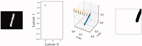
We also confirmed that participants were able to draw sketches that enabled accurate target classification. Figure 8 depicts the AMT interface presented to participants, as well an encoding and sketch a participant drew in response to an MNIST image and a motion trajectory. The sketch encoding is particularly impressive. Converting the sketch into a 16 × 16 pixel drawing and passing it through the predictor model led the model to predict the correct target: location 0. It is noteworthy that participants created reasonable encodings of the trajectories instead of merely adopting the approach of generating the simplest encoding that would create the correct classification. For example, the participant who generated the sketch depicted in Figure 8 could have drawn a very short sketch near target location 0 but instead opted to draw a longer line, reflecting the length of the original trajectory. This indicates that participants truly were encoding inputs in much the same way that the models did.

Figure 8. Participants successfully converted MNIST images to 2 D encodings (left) and trajectories into sketches (right). (a) PAE. (b) PCN. (c) OSP by parity. (d) ASP by parity. (e) ASP by digit.

12. Assessing trust calibration

In our final experiment, we wished to measure a new aspect of human-machine alignment: trust calibration. Just as a semantic measure of alignment was possible because of specific characteristics of robot-robot alignment, using humans in a team allowed us to measure characteristics of alignment that only humans could report. In this experiment, we focused on the notion of trust. Trust, defined by Lee and See as “the attitude that an agent will help achieve an individual’s goals in a situation characterized by uncertainty and vulnerability,” is commonly used as a metric of human-agent interaction; good interactions are characterized by enabling humans to understand the extent to which they should or should not rely upon a machine (Lee & See, 2004; Wang et al., 2018). In this experiment, we assumed that an individual’s goal was correct classification of an input, so trust was reflected in participants’ belief that an agent would correctly classify the input.

This experiment was conducted via surveys on AMT, using the same models that had been trained for the previous human-agent experiments. Consistent with the earlier surveys, participants were initially presented with a summary of how the machine worked and some (input, latent, prediction) examples. After reading the prompt, participants were asked 10 questions. In each question, participants were shown an input (e.g., an MNIST image) and a representation (e.g., a point in a 2 D latent space) and asked to rank their confidence from 0 to 100 that the machine would make the correct prediction (e.g., the digit in the image).

After a participant submitted a response to each question, they were shown whether the machine had indeed made the correct classification for the previous case and were presented with the examples from the instruction prompt to refresh their memories. Of the 10 (randomly ordered) questions shown, 5 resulted in the machine making a mistake, while the remaining 5 yielded a correct classification. This artificially low 50% accuracy rate allowed us to better measure participants’ anticipation of failures.

After recording the participants’ responses, we analyzed the data by measuring their trust calibration coefficients. We defined this coefficient as the slope of the linear least-squares fit for plotting model correctness (1 for correct, 0 for incorrect) over participants’ confidence. Perfectly calibrated trust would result in a slope of 0.01, corresponding to high participant confidence when the model was correct and low confidence when it was incorrect. Recall that trust calibration, as opposed to simply high trust, is a desirable property of human-robot interaction (Wang et al., 2018).

The trust calibration coefficients, multiplied by 100 for clarity, were recorded in Table 4. In three of the four tasks, at least one of the latent types yielded significantly positive coefficients (p < 0.05). Results from the parity task, by far the simplest of the four, demonstrated that participants were able to establish well-calibrated trust for a large number of latent spaces. For the digit and target tasks, only one latent space yielded significant correlation. For the intersection task, we were only able to establish significant positive correlation for the ASP sketch at the level of (p < 0.1). These results supported several conclusions.

Table 4. Trust coefficients multiplied by 100 for different tasks and latent types.

Task	ASP dig.	ASP par.	OSP dig.	OSP par.	PAE	PCN
Parity	0.24 (70)	0.56* (130)	_	0.49* (110)	0.06 (100)	0.37* (90)
Digit	0.47* (110)	0.01 (130)	0.18 (80)	_	0.13 (120)	0.27 (80)
	ASP 2D	ASP sketch	OSP 2D	OSP sketch	PAE	PCN
Inter.	−0.04 (40)	0.39 (100)	_	−0.13 (40)	0.22 (80)	0.20 (90)
Target	−0.02 (60)	0.43* (70)	0.04 (120)	_	0.11 (90)	0.26 (70)

A value of 1 corresponds to perfectly calibrated trust. Coefficients significantly greater than 0 (p < 0.05) are denoted with *. The number of question responses is noted in parentheses.

First, we demonstrated once again that the utility of latent space designs was task-dependent. Consider the values for the parity and digit prediction tasks using the ASP digit and ASP parity latent spaces; clustering by parity was optimal for the parity prediction task, but clustering by digit was optimal for the digit prediction task. This reversal of optimality establishes that we observed no “dominating” latent designs that were always better, independent of task.

Second, we performed analysis of covariance (ANCOVA) and established significant effects of latent type on participants’ confidence. Specifically, we treated confidence as a dependent variable and model correctness and latent type as explanatory variables. For all four tasks, the latent type categorical variable had a significant effect on user confidence (p < 0.05). The significance of the interference between latent type and correctness, however, was less definitive: for the parity and digit tasks the interference was significant at p < 0.05, for target at p < 0.15, and was not significant for the intersection task. In other words, the latent type clearly shifted participants’ confidence up or down but did not consistently change the slope of the trust models for all tasks.

13. Analysis review

In the previous sections, we presented the results and analysis for each of the experiments we conducted. In this section, we briefly review the three key findings from all the experiments taken together.

First, the pragmatic metric appeared to be a faithful, but conservative, proxy of semantic latent space alignment. In measuring both metrics for the same robot-robot teams, we found that the two measures were correlated. Furthermore, we found that the semantic measure appeared to be the more sensitive of the two metrics, but our pragmatic metric could be used in more experiments, including those with human participants.

Second, we found that techniques that used human guidance in learning latent spaces (i.e., OSP and ASP) outperformed unguided techniques, as well as a technique borrowed from interpretability research. Furthermore, in a series of experiments for different tasks, model architectures, and latent space designs, we found that ASP outperformed OSP.

Third, we confirmed that, when using latent space designs in training new models, the utility of particular designs was task specific. For example, designs that clustered MNIST encodings by digit were most useful for digit classification tasks, but less useful for parity prediction tasks.

14. Related work

In addition to the two specific techniques taken from prior art (OSP and PCN) our work is closely related to work from numerous fields. First, notions of conforming to expected behavior and learning social conventions is explored in research on norms emergence. Second, insights from imitation learning indicate how demonstrations may be used to guide learned behaviors. Third, work in creating interpretable models that humans understand is often motivated by the same desire as our work in aligning latent spaces, but specifically in the context of aligning with human models. Lastly, although research in ontology matching often uses different techniques than the ones we employed, the motivation of mapping between representation schemes is related to the problem of latent space alignment.

14.1. Social conventions and norm learning

In this work, we implemented a specific technique, OSP, for learning social conventions and drew inspiration from the broader field of norm learning (Lerer & Peysakhovich, 2018).

Researchers on norm emergence have long studied how norms—expectations of behavior among a population of agents—are formed, diffuse through populations, or may be guided by particular “influencer” agents (Franks et al., 2013; Savarimuthu & Cranefield, 2011; Sen & Airiau, 2007; Verhagen, 2001). Our framing of latent space alignment is related to commonality of behavior, and in particular our adversarial approach of training in ASP vaguely resembles the notion of sanctions in norm learning literature (Andrighetto et al., 2010). Focusing on individual agents instead of network effects, other work has explored how to train a new agent to collaborate successfully with pre-trained partners (Barrett et al., 2017; Stone et al., 2010).

These techniques offer important insight into training specific agent behaviors, but our work differs in several important ways. First, we examine the importance of representation, as opposed to behavioral, alignment. Second, unlike many of the techniques in norm learning (with the notable exception of OSP), ASP does not required interaction with other agents during training time (Lerer & Peysakhovich, 2018). Lastly, the experiments conducted in this work demonstrate latent space alignment both with other agents and with other humans.

14.2. Imitation learning

In contrast to the agent-centric focus of norm learning, imitation learning work often attempts to train new agents to learn a policy from a human teacher by way of demonstrations of optimal behavior (Argall et al., 2009). Numerous approaches to imitation learning have been proposed from policy cloning, wherein behavior learning is cast as a supervised learning problem, to inverse reinforcement learning (IRL), wherein agents attempt to learn the teacher’s reward function, which may then be used to calculate an optimal policy (Abbeel & Ng, 2004; Pomerleau, 1991). In recent years, adversarial techniques have even been applied to imitation learning by training an adversary to discriminate between expert and learned behaviors (Ho & Ermon, 2016; Li et al., 2017).

These techniques are related to our use of paired and unpaired data in training new agents to learn a specific representation function. However, imitation learning often leverages notions of environment reward instead of our classification contexts. In addition, our framing of latent space alignment in order to enable high mixed-team task performance differs from the standard imitation learning goal of teaching an agent to perform a task on its own.

14.3. Model interpretability

Much like the agent-focused literature of norm learning, interpretable representation learning is related to our work, although it often only considers human partners. As stated earlier, we used PCN as a baseline against which to compare the methods we implemented (Li et al., 2018). More broadly, however, the idea of interpretable machine learning models corresponds to some extent with aligning with human mental models.

Some interpretability approaches yield explanations that describe complex models without actually modifying them. For example, Ribeiro et al. and Lundberg and Lee created linear models to locally approximate a complex decision boundary (e.g., a neural net’s classification boundary) (Lundberg & Lee, 2017; Ribeiro et al., 2016). However, such post-hoc techniques do not reflect the underlying decisions or representations of the model being explained. This poses both theoretical and real challenges: the disconnect between explanations and truth is troubling and can be exploited to generate incorrect explanations (Rudin, 2018; Slack et al., 2020).

Other researchers have taken a different approach by changing models to facilitate interpretation. Prior work in disentanglement separated representations within neural nets into composable representations (Higgins et al., 2017; Mathieu et al., 2016; Ridgeway & Mozer, 2018); however, while such methods achieve theoretical disentanglement, the representations are not guaranteed to align with human intuition. In fact, the cases in which disentangled representations match human notions appear to be due primarily to inductive biases and parameter tuning rather than theoretical guarantees (Locatello et al., 2019). With the introduction of labeled data, other techniques have managed to remove information from representations to create “fair” predictors that ignore protected input attributes, but such techniques only define what information representations should not include (Louizos et al., 2016). Still other work has incorporated case-based reasoning as a building block of interpretable models (Chen et al., 2019; Kim et al., 2014; Li et al., 2018).

Recent work also suggests the importance of model interpretability in enabling effective human-agent interaction. The three levels of situational awareness defined by Endsley (Endsley, 2011)—perception, comprehension, and projection—suggest that prediction of an agent’s next action is enhanced by facilitating the human’s understanding of that agent’s current state and functionality. In addition, Sanneman and Shah formally established the connection between interpretability methods and situational awareness (Sanneman & Shah, 2020).

Our work differs from traditional interpretability research in two ways. First, we focused on representation learning specifically, rather than studying all aspects of a model’s behavior. Second, our formulation of latent space alignment was not restricted to only partnering with humans. Instead, we generalized the problem of learning alignments and treated humans just one of many possible partners.

14.4. Ontology matching

Ontology matching “aims at finding correspondences between semantically related entities of different ontologies” (Euzenat et al., 2007). More intuitively, this means finding a mapping between two sets of labels that refer to the same objects. For example, two different languages like French and English have different words for the same concepts; a French-English translator provides a way of converting from one to another.

Roboticists and AI researchers have long understood the importance of ontology matching to help heterogeneous agents communicate, including (Trojahn et al., 2011; Van Eijk et al., 2001; Wiesman et al., 2002), among others. These various works offer solutions to mapping between the ontologies of two or more pre-trained agents.

While we appreciate the motivation of reconciling model ontologies, our approach differs in because, rather than starting with pre-trained agents with fixed ontologies and deducing a mapping between them, our approach is used in training the agents themselves.

15. Contributions

In this article, we took a step towards fluent robot teamwork by enabling agents to align their internal representations with that of a partner, whether human or machine. We introduced a new, data-efficient mechanism for latent space alignment that trained models using as little as 8 examples of their partner’s representation for particular inputs. Two proposed metrics of latent space alignment provided a measure of compatibility between agents, which we used to compare our technique to others from social convention and interpretability literature. In studies of machine partnerships, we identified the utility of learning the latent space of a pre-trained agent and noted the improvements our technique afforded. Human participant studies similarly demonstrated that our technique enabled models to learn simple human conventions, resulting in better human-agent team performance.

The findings from this article indicate promising avenues for future research. First, more extensive user studies could measure ASP’s ability to train models that conform to a personalized latent space designed by participants. That is, rather than use the researcher-generated latent designs, participants could create designs according to their own preference. Second, this work demonstrated the importance of good latent designs for human comprehension: further research into characteristics of good designs could support the application of this technique in a wide variety of settings. Lastly, the high-level lesson of this article—that self-play, conforming to a distribution, and a small amount of paired data can efficiently train agents to adopt a protocol—is widely applicable. I would be delighted to see this technique adopted in the fields of natural language processing, for example: information would be passed through words, those words must reflect the distribution of words from the language, and a dictionary could provide the meanings or groundings of the words.

Disclosure statement

No potential conflict of interest was reported by the author(s).

Correction Statement

This article has been republished with minor changes. These changes do not impact the academic content of the article.

Additional information

Notes on contributors

Mycal Tucker

Mycal Tucker is a PhD student at MIT working on cognitively-inspired neural network models for human understanding. His research includes methods for designing interpretable neural network architectures, enabling human-understandable emergent communication, and uncovering underlying principles in large neural models.

Yilun Zhou

Yilun Zhou is a PhD student at MIT working on the interpretability and transparency of learned (and especially black-box) models. His research develops algorithms to improve human’s understanding of a model and methods to critically evaluate quantify existing claims of interpretability.

Julie A. Shah

Julie A. Shah is a Professor of Aeronautics and Astronautics at MIT, and directs the Interactive Robotics Group in the Computer Science and Artificial Intelligence Laboratory. Her lab aims to imagine the future of work by combining human cognitive models with artificial intelligence in collaborative machine teammates that enhance human capability.

Appendix A.

Learned latent spaces from designs.

In Section 10, we explained the set of experiments wherein models were trained to align with latent space designs. Figures of the designs were included in the main text, but the patterns that the models themselves learned were plotted below. That is, Figures A1–A3 are visualizations of the latent spaces that the model learned, which in turn sheds light on the relative strengths of different designs and training techniques. (Given that the learned latent spaces for the intersection and target tasks were quite similar, only the latent spaces for the target task were plotted.)

Figure A1. Parity task. (a,b) The autoencoder and PCN networks created clusters by parity, but at surprising orientations. OSP (c) and ASP (d) both allowed for human guidance to move even numbers into a rectangle on the left and odd numbers into a rectangle on the right—although ASP resulted in sharper divisions between groups. Creating clusters by digit in a dialpad pattern was possible but overly complex for predicting parity (e). (a) PAE. (b) PCN. (c) OSP by digit. (d) ASP by digit. (e) ASP by parity

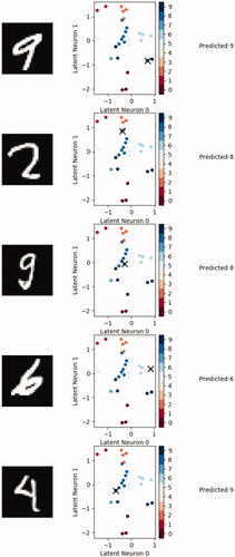
Figure A2. Digit task. (a,b) The autoencoder and PCN networks created clusters by digit but in an unintuitive layout. OSP (c) and ASP (d) both allowed for human guidance to move those clusters into a telephone grid, but ASP resulted in sharper divisions between clusters. Using the parity clusters from earlier remained possible but was less useful (e). (a) PAE. (b) PCN. (c) OSP by parity. (d) ASP by parity. (e) OSP sketches. (f) ASP sketches. (g) PCN sketches.

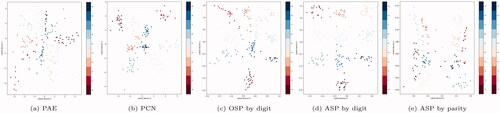
Figure A3. Target task. (a–d) In the top row, 2 D encodings of trajectories form patterns by target bolt, but OSP and ASP imposed a ray structure. (e–g) 16 × 16 encodings of trajectories turned into sketches for OSP and ASP, but unsupervised approaches look like noise.

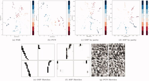
Consistent patterns were apparent in learned latent spaces. First, techniques that did not use data from designs often learned surprising or unintuitive latent spaces. For example, clusters of MNIST digits were arranged in an unexpected layout, and sketch-based encodings resembled noisy pixels instead of clear lines. Second, ASP generated “sharper” learned representations than OSP did. For 2 D latent spaces, that meant clearer divisions between clusters of encodings; for sketches, that led to fewer gray pixels and more continuous dark lines.

Appendix B.

Survey prompt

The following prompt was shown to AMT participants at the start of a survey assessing trust calibration for the digit prediction task:

In this task, we will ask you questions to determine if you can figure out the “language” the computer uses to solve pattern matching problems.

In the same way that an English speaker and a French speaker will use different words or phrases to talk about the same object, machines that use artificial intelligence learn their own sorts of representations of objects.

These representations are typically a series of numbers instead of words, but they have meaning to the machines nonetheless. Just like an English speaker who hasn’t studied French may not know what a French speaker is saying, humans often have trouble understanding the representations of machines. If we want to rely upon or work with machines, though, we would like to make sure that we can understand what representations they are using. If we can understand a machine’s language, we can better judge whether it is making good or bad decisions.

In this survey, you and a machine see a series of images of hand-drawn digits (e.g., a photo of someone who wrote the number 8). Our machine generates some numbers as its representation of the image. You may think of those numbers sort of like words. The machine then runs some computations on those numbers and tries to figure out what digit was originally drawn in the image.

A useful analogy for this computation process is the game of “telephone.” First, imagine that a person looks at an image and thinks of a few words. That first person then says those words to a second person who has to figure out what was in the image. The machine converts an image to a representation and then the representation to a decision on the digit. For example, if the machine sees an image of a handwritten 8, it converts that image into a representation of its choice and then, based on the representation, the machine says that there was an 8 in the image. The machine plays this game of telephone so that it can learn a general representation of an eight (like it is made up of two zeros stacked on top of each other), rather than simply memorizing the answer for every single picture it sees.

Unfortunately, our machine isn’t perfect. What we would like to measure in this experiment is whether humans can tell when the machine is going to mess up. You will be shown an image of a digit and the representation that the machine generated, and your job will be to say how confident you are that the machine will predict the correct digit. If the machine spoke English, this would be easy: if you saw an image of a 8 but the representation said “it’s a 7,” you could say that the machine will probably mess up.

Because the machine doesn’t speak English, below are some examples of how the machine has behaved in the past; these examples can help you learn what the machine’s representations mean.

In the column on the left, you see images of handwritten digits. In the middle column, you see figures that depict information about the machine’s representations. Pay attention to the location of the X in the figure. Its location is the representation that the machine uses for the image of the handwritten digit on the left. That’s why, when the image of the handwritten digit changes in different rows, the X moves to different locations. All the colorful points in the figures with the X’s are just a way of showing extra information: the locations of the points were generated by tracking the X’s for other images, and then each point was colored by what digit the machine thought was in the image. For example, if the machine represents an image as an X right in the middle of the figure and predicts that the image is the digit 0, you will see a dark red dot in the middle of the figure (using the colorbar as shown in the figures below). Lastly, in the right column, you see what digit the machine thought was in the image based on the location of the X.

In this survey, you will be shown an image of a hand-written digit and the representation that the machine generated for that image, and you will be asked how confident you are that the machine will correctly predict the digit in the image. After answering the question, you will be told whether the machine was correct or not for the case you just saw. You will also be asked to answer a question about how confident you are about the performance of the machine overall (instead of just for one particular image). For example, even if there are some scenarios where you think the machine is very accurate, but you think that most of the time it will make a mistake, you might say that you are no.

References

- Abbeel, P., & Ng, A. Y. (2004). Apprenticeship learning via inverse reinforcement learning [Paper presentation]. Proceedings of the Twenty-First International Conference on Machine Learning (p. 1). https://doi.org/10.1145/1015330.1015430
- Andrighetto, G., Villatoro, D., & Conte, R. (2010). Norm internalization in artificial societies. AI Communications, 23(4), 325–339. https://doi.org/10.3233/AIC-2010-0477
- Argall, B. D., Chernova, S., Veloso, M., & Browning, B. (2009). A survey of robot learning from demonstration. Robotics and Autonomous Systems, 57(5), 469–483. https://doi.org/10.1016/j.robot.2008.10.024
- Barrett, S., Rosenfeld, A., Kraus, S., & Stone, P. (2017). Making friends on the fly: Cooperating with new teammates. Artificial Intelligence, 242(1), 132–171. https://doi.org/10.1016/j.artint.2016.10.005
- Breazeal, C., Gray, J., & Berlin, M. (2009). An embodied cognition approach to mindreading skills for socially intelligent robots. The International Journal of Robotics Research, 28(5), 656–680. https://doi.org/10.1177/0278364909102796
- Chen, C., Li, O., Barnett, A., Su, J., & Rudin, C. (2019). This looks like that: Deep learning for interpretable image recognition [Paper presentation]. Proceedings of Neural Information Processing Systems (NeurIPS).
- Chollet, F., et al. (2015). Keras. GitHub.
- Endsley, M. R. (2011). Designing for situation awareness: An approach to user-centered design (2nd ed.). CRC Press.
- Euzenat, J., & Shvaiko, P. (2007). Ontology matching (Vol. 18). Springer.
- Franks, H., Griffiths, N., & Jhumka, A. (2013). Manipulating convention emergence using influencer agents. Autonomous Agents and Multi-Agent Systems, 26(3), 315–353. https://doi.org/10.1007/s10458-012-9193-x
- Frawley, W. (2013). Linguistic semantics. Routledge.
- Hernandez-Leal, P., Kartal, B., & Taylor, M. E. (2019). A survey and critique of multiagent deep reinforcement learning. Autonomous Agents and Multi-Agent Systems, 33(6), 750–797. https://doi.org/10.1007/s10458-019-09421-1
- Hiatt, L. M., Narber, C., Bekele, E., Khemlani, S. S., & Trafton, J. G. (2017). Human modeling for human–robot collaboration. The International Journal of Robotics Research, 36(5–7), 580–596. https://doi.org/10.1177/0278364917690592
- Higgins, I., Matthey, L., Pal, A., Burgess, C., Glorot, X., Botvinick, M. M., Mohamed, S., & Lerchner, A. (2017). beta-vae: Learning basic visual concepts with a constrained variational framework. Under review as a conference paper at ICLR 2017.
- Ho, J., & Ermon, S. (2016). Generative adversarial imitation learning. Advances in Neural Information Processing Systems, 29, 4565–4573. https://doi.org/10.48550/arXiv.1606.03476
- Huang, S. H., Held, D., Abbeel, P., & Dragan, A. D. (2019). Enabling robots to communicate their objectives. Autonomous Robots, 43(2), 309–326. https://doi.org/10.1007/s10514-018-9771-0
- Iqbal, T., Gonzales, M. J., & Riek, L. D. (2015). Joint action perception to enable fluent human-robot teamwork [Paper presentation]. 2015 24th IEEE International Symposium on Robot and Human Interactive Communication (RO-MAN) (pp. 400–406). IEEE. https://doi.org/10.1109/ROMAN.2015.7333671
- Kim, B., Rudin, C., & Shah, J. (2014). The bayesian case model: A generative approach for case-based reasoning and prototype classification. In Proceedings of the 27th International Conference on Neural Information Processing Systems – Volume 2, NIPS'14 (pp. 1952–1960). MIT Press.
- Kingma, D. P., & Welling, M. (2014). Auto-encoding variational bayes. In Y. Bengio & Y. LeCun (Eds.), 2nd International Conference on Learning Representations, ICLR 2014, Banff, AB, Canada, April 14-16, 2014, Conference Track Proceedings.
- Lee, J. D., & See, K. A. (2004). Trust in automation: Designing for appropriate reliance. Human Factors, 46(1), 50–80. https://doi.org/10.1518/hfes.46.1.50_30392
- Lerer, A., & Peysakhovich, A. (2018). Learning existing social conventions via observationally augmented self-play [Paper presentation]. Proceedings of the 2019 AAAI/ACM Conference on AI, Ethics, and Society.
- Li, O., Liu, H., Chen, C., & Rudin, C. (2018). Deep learning for case-based reasoning through prototypes: A neural network that explains its predictions. In Proceedings of the Thirty-Second AAAI Conference on Artificial Intelligence (AAAI) (pp. 3530–3537). AAAI.
- Li, Y., Song, J., & Ermon, S. (2017). Infogail: Interpretable imitation learning from visual demonstrations. Advances in Neural Information Processing Systems, 30, 3812–3822. https://doi.org/10.48550/ARXIV.1703.08840
- Locatello, F., Bauer, S., Lučić, M., Rätsch, G., Gelly, S., Schölkopf, B., & Bachem, O. F. (2019). Challenging common assumptions in the unsupervised learning of disentangled representations. ICLR. (pp. 4114–4124). PMLR.
- Louizos, C., Swersky, K., Li, Y., Welling, M., & Zemel, R. (2016). The variational fair autoencoder. In Y. Bengio & Y. LeCun (Eds.), ICLR. http://arxiv.org/abs/1511.00830
- Lundberg, S. M., & Lee, S.-I. (2017). A unified approach to interpreting model predictions. In I. Guyon, U. V. Luxburg, S. Bengio, H. Wallach, R. Fergus, S. Vishwanathan, & R. Garnett (Eds.), Advances in neural information processing systems (Vol. 30, pp. 4765–4774). Curran Associates, Inc.
- Mathieu, J. E., Heffner, T. S., Goodwin, G. F., Cannon-Bowers, J. A., & Salas, E. (2005). Scaling the quality of teammates’ mental models: Equifinality and normative comparisons. Journal of Organizational Behavior, 26(1), 37–56. https://doi.org/10.1002/job.296
- Mathieu, M. F., Zhao, J. J., Zhao, J., Ramesh, A., Sprechmann, P., & LeCun, Y. (2016). Disentangling factors of variation in deep representation using adversarial training. In D. D. Lee, M. Sugiyama, U. V. Luxburg, I. Guyon, & R. Garnett (Eds.), Advances in neural information processing systems (Vol. 29, pp. 5040–5048). Curran Associates, Inc.
- Nikolaidis, S., & Shah, J. (2013). Human-robot cross-training: Computational formulation, modeling and evaluation of a human team training strategy [Paper presentation]. 2013 8th ACM/IEEE International Conference on Human-Robot Interaction (HRI) (pp. 33–40). https://doi.org/10.1109/HRI.2013.6483499
- Pomerleau, D. A. (1991). Efficient training of artificial neural networks for autonomous navigation. Neural Computation, 3(1), 88–97. https://doi.org/10.1162/neco.1991.3.1.88
- Ramakrishnan, R., Kamar, E., Dey, D., Horvitz, E., & Shah, J. (2020). Blind spot detection for safe sim-to-real transfer. Journal of Artificial Intelligence Research, 67, 191–234. https://doi.org/10.1613/jair.1.11436
- Ribeiro, M. T., Singh, S., & Guestrin, C. (2016). “Why should I trust you?”: Explaining the predictions of any classifier. In Proceedings of the 22nd ACM SIGKDD International Conference on Knowledge Discovery and Data Mining, KDD '16 (pp. 1135–1144). Association for Computing Machinery.
- Ridgeway, K., & Mozer, M. C. (2018). Learning deep disentangled embeddings with the f-statistic loss. In S. Bengio, H. M. Wallach, H. Larochelle, K. Grauman, N. Cesa-Bianchi, & R. Garnett (Eds.), Proceedings of neural information processing systems (NeurIPS) (pp. 185–194). NIPS.
- Rudin, C. (2018). Stop explaining black box machine learning models for high stakes decisions and use interpretable models instead. Nature Machine Intelligence, 1, 206–215. https://doi.org/10.1038/s42256-019-0048-x
- Sanneman, L., & Shah, J. A. (2020). A situation awareness-based framework for design and evaluation of explainable AI. In International workshop on explainable, transparent autonomous agents and multi-agent systems (pp. 94–110). Springer.
- Savarimuthu, B. T. R., & Cranefield, S. (2011). Norm creation, spreading and emergence: A survey of simulation models of norms in multi-agent systems. Multiagent and Grid Systems, 7(1), 21–54. https://doi.org/10.3233/MGS-2011-0167
- Sen, S., & Airiau, S. (2007). Emergence of norms through social learning. In IJCAI (pp. 1507–1512).
- Slack, D., Hilgard, S., Jia, E., Singh, S., & Lakkaraju, H. (2020). Fooling lime and shap: Adversarial attacks on post hoc explanation methods [Paper presentation]. Proceedings of the AAAI/ACM Conference on AI, Ethics, and Society, AIES '20 (pp. 180–186). Association for Computing Machinery.
- Stone, P., Kaminka, G. A., Kraus, S., & Rosenschein, J. S. (2010). Ad hoc autonomous agent teams: Collaboration without pre-coordination. In Proceedings of the Twenty-Fourth AAAI Conference on Artificial Intelligence, AAAI (Vol. 10, pp. 1504–1509). AAAI Press.
- Trojahn, C., Euzenat, J., Tamma, V., & Payne, T. R. (2011). Argumentation for reconciling agent ontologies. In Semantic agent systems (pp. 89–111). Springer.
- Van Eijk, R. M., De Boer, F. S., Van der Hoek, W., & Meyer, J.-J C. (2001). On dynamically generated ontology translators in agent communication. International Journal of Intelligent Systems, 16(5), 587–607. https://doi.org/10.1002/int.1025
- Verhagen, H. (2001). Simulation of the learning of norms. Social Science Computer Review, 19(3), 296–306. https://doi.org/10.1177/089443930101900305
- Wang, C., Zhang, C., & Yang, X. J. (2018). Automation reliability and trust: A Bayesian inference approach. Proceedings of the Human Factors and Ergonomics Society Annual Meeting, 62, 202–206. https://doi.org/10.1177/1541931218621048
- Wiesman, F., Roos, N., & Vogt, P. (2002). Automatic ontology mapping for agent communication. In Proceedings of the First International Joint Conference on Autonomous Agents and Multiagent Systems: Part 2 (pp. 563–564). ACM.