How to Create an Area When Playing against a Machine

Abstract

How would human players negotiate a spatial array with a randomly behaving partner? In an interactive, online, zero-sum grid game, we tested whether and how players create areas and place sequences by coloring-in places in a 20 × 20 matrix (261 human adults, 261 machine partners, N = 522). Several indicators showed that human players followed an intentional strategy rather than coloring in places ad libitum. First, human players built a larger largest cluster from places than the machine. Second, they were sensitive to task instructions and could modify their strategy accordingly. When instructed to build an area, they built a bigger one. When set under time pressure, they colored-in faster and only had time to build a smaller cluster from places. Third, the most compelling human strategy to create an area was lining up pathways (place sequencing). Despite these differences, the resulting spatial field structure was similar in human and machine players.

1. Introduction

The current study addresses the cognitive aspects of interactive computing when playing an online board game. For many centuries, people have been playing interactive board games like chess and Go using various types of matrices and spatial rules. These games are usually played in pairs and are often competitive (Gobet et al., 2004; Nash, 1951). Moreover, such board games can be played against the computer system and machine algorithms that were programmed to beat expert human players (Silver et al., 2016). The current study presents a new type of an interactive online board game where the locations of a grid matrix are colored-in by each game partner taking turns, with players using a different color to create areas by adjacent same-colored places. The computer was programmed to behave randomly in this interaction, and we analyzed how human players would respond, that is, whether they would also behave randomly, or would deploy specific strategies.

1.1. Space, area and pathways in space

Overall pictorial space is usually conceptualized with spatial axes, with a clear human development from implicit space with just objects, to one-dimensional horizontal axes structures, to orthogonal and viewpoint areas (Lange-Küttner, 2009). It has been argued that the transition from implicit space, with just objects, to three-dimensional Euclidian space approximates the contained objects to numerical entities that have their place denoted in space but reduces the relevance of their shape (Lange-Küttner, 1997, 2004). Grid structures are rarely used in depictions of natural scenes unless they mark a pattern on the floor. It is much more common to see beaches with a horizontal axis or roads as spatial pathways leading to viewpoints (Anderson et al., 2021) than to find grid patterns. Moreover, a comparison between a frame and a grid array in comparison to an implicit empty space showed that the boundaries of a frame narrowing down a search area were more effective for spatial memory than a grid denoting each place (Lange-Küttner, 2013).

Nevertheless, grid structures were used to concentrate on small sections when transforming a three-dimensional model into a two-dimensional drawing on paper. Grid structures are also used for city planning and arithmetical calculations on paper. Grids enable to create random dot stereograms (Julesz, 1971) and QR codes (Szentandrási et al., 2012). Moreover, also in artificial intelligence (AI) grids provide structure. Pixelated images make it hard for machine vision to identify real objects and thus there exists a longstanding research stream of object recognition approaches that suggest to use either object-based compilations of sophisticated “building bricks” like geons (Biederman, 1987, 2000), or edge and contour extraction by contrast detection that optimizes the natural and visually realistic silhouette (Marr et al., 1980). In virtual (VR) and augmented (AR) reality, grid mesh covers rudimentary objects and provides visually realistic surfaces that denote object contours. It is also possible to detect areas of visual planes in pixelated images by connecting pixels into lines in a 2 D graph providing a topological map (Bhargav et al., 2019), but they are hard to detect in cluttered spaces. Thus, neutral visual code markers are used that function like landmarks to denote reference points for a visual field (Bhargav et al., 2019). Also in living organisms, mental representations consisting of grid cells provide a Euclidian spatial metric (Krupic et al., 2016). Krupic et al. also distinguish between a local and a global grid; they claim that a global grid gradually integrates local grids. The more complex the global shape, the longer it would take to make this overall shape regular, without local distortions. While the grid cells are located in the entorhinal cortex, the door to long-term memory, place cells are located in the hippocampus proper (Krupic et al., 2016). Neural network simulations allowed to specify the amount of place cells, grid cells and boundary cells that facilitate to maneuver a maze (Banino et al., 2018). They found that between 21.4% to 25% involved grid-like units, 10.2% were head direction cells, 8.7% border cells and only a small number were place cells. Only grid cells were able to generalize to larger arrays. One would assume that place cells need to be transformed into larger units in order to become effective. Thus, the grid is an important geometric structure that helps in various domains of life, at different levels, from the behavioral to the graphic, to the simulated and physiological neural level.

1.2. Competitive space in board games

Since the advent of field theory in Psychology, the question is how such spatial fields are dynamically constructed. Tolman (1948) and Lewin (1936) have been instrumental in field theory. In one short paper, their differences were clearly denoted (Lewin, 1933). While both authors were using a spatial field with obstacles to an aim, Tolman used ready-made mazes and analyzed the factors that would lead to pathway choices in order to reach the aim, but Lewin was interested in how the field itself became structured by the protagonists being caught up in positive and negative valences and field forces. The direction and strength of the field force were denoted with vectors that Lewin thought would make his model suitable for mathematical computation. A field would not exist a priori, but is dynamically created and delimited into several topological regions (Lewin, 1936). One problem could be whether the different regions in such a structured field would be additive or nested. Another issue was whether a certain valence could be attached to the space that would qualify a region, for instance, as a negative “alien space” or a positive “freedom space,” translating into field forces. A recent approach is a purely perceptual analysis of common regions that are created by explicit spatial boundaries which can supersede the well-known Gestalt grouping principles of proximity and similarity that involve just shapes (Lange-Küttner, 2006; Palmer, 1992).

Humans have been working with such spatial scenarios since centuries, beginning with board games that employ a grid and that were further developed into more natural scenarios in virtual reality games. Gobet et al. (2004) defined games like Chess and Go as “war games” because the focus would be on the annihilation of the opponent in comparison to “race games” where the aim is on oneself to be first arriving at a goal. Chess makes it possible to remove enemy officers when they land in the same place, but the ultimate goal is to deprive the king of his freedom of movement (checkmate), delimiting his freedom space. In Go, however, the goal is to maximize “land ownership” by closing, encircling and deleting the opponent's stone or sequence of stones, taking over alien space. Furthermore, in “alignment games,” the objective is to complete a prescribed configuration.

Chess could be expected to be the most difficult board game due to the various ranks of figures and their roles, but this is not the case. The board game software “Deep Blue” beats Chess masters since 1997, but Google’s Deep Mind “Alpha Go” was beating Go masters only 18 years later (Silver et al., 2016). This late success proves that Go was the most difficult game for AI even though the pieces are simple and uniform and have no different functions like chess figures. The greater challenge of Go for AI is that while chess consists of an 8 × 8 grid with clearly distinguishable individual black and white places, the Go board has a larger 19 × 19 grid with places that are all the same color. A larger grid provides greater freedom and less spatial constraints to select a location. A larger grid thus requires more computing power to explore all possibilities of potential moves, a process that is called “brute force” in comparison to a “heuristic” which consists of a simpler strategy that is more economical in terms of computing power (Gobet et al., 2004). One such heuristic could be to focus on a small region within an array, another heuristic to focus on several regions, and yet another one could be to make random moves and capitalize on the mistakes of the opponent.

1.3. The current study

In the current study, we are testing how places and regions are dynamically created with a randomly behaving partner. Participants are taking turns with the machine system when each is coloring-in two hundred places in a 20 × 20 grid array with 400 places in total. The grid array is not an unstructured field insofar as each place in the grid is clearly delineated by a boundary. Each of the two players uses their own, different color, and can merge places that they color-in with the same color into a region. In this way, a player could create regions carrying their color within the spatial field of the grid that supersede the individual places. There were no barriers, but the opponent player could interfere with a plan to create a region in a particular part of the spatial field. Especially the machine with its random behavior could interfere with human plans, while humans would find it harder to interfere with the machine as there was no strategy except for random spatial exploration. There was no aim apart from carrying on until the entire grid was colored in, that is, until the creation of regions was so advanced that no places were left and all were belonging to one or the other player, respectively. There was no gain to be made or reward to be obtained as each player could only color-in exactly half of the 400 places. In this sense, even if no territorial gains could be made, the game was competitive insofar as plans for a region could be counteracted. In short, an online, interactive and dynamic, zero-sum grid game was played that involved participants to create their own places and regions in a spatial field by marking them in their allocated color.

There was a crucial difference between the two players, though: While the human participants could devise their own strategies, the machine was programmed to color in places randomly as this would maximise spatial exploration. The size of the players’ areas was measured in terms of the number of places that were merged. For the machine, a large area could only emerge incidentally because of the random way the machine colored-in places. To prove that adults really controlled the creation of an area, four different instructions were devised in order to assess whether adults could systematically modify their coloring-in behavior. One group of participants was asked to work quickly and set under time pressure that would disrupt their planning with a smaller large area as a result. Another group of participants was given an explicit prescription to build an area with as much time as they liked so that they could build a larger large area. Another third group was given both instructions, to work quickly and to create a large region. Here it was expected that the size of their areas would be between the other two groups as the two instructions would neutralize each other and hence the effect should be nil in comparison to the control group without an additional instruction.

In the task, the humans would touch a place with a finger or click into a place with a computer mouse and the place would fill with green color, see Figure 1, followed by the machine filling in a random place with yellow color.

Figure 1. Coloring-in of a 20 × 20 grid. Note. green = human (dark grey); yellow = machine (light grey); black = empty.

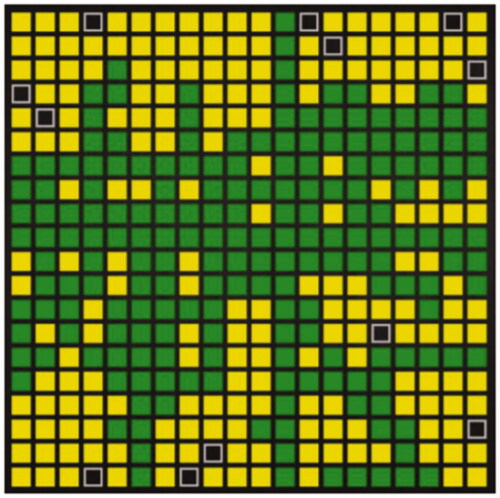
It was not mentioned to participants that the machine as the interactive game partner would color-in places in a random fashion—although players could of course quickly realize that this was the case. Sensitivity to instruction would indicate that the participants were using a flexible strategy rather than some reflex following the randomly behaving machine opponent. Instead the machine in a way “followed” the lead of the human players (Turing, 1950). However, a sensible perceptual pattern can also occur by chance (Bar-Hillel & Wagenaar, 1991). Another factor which may get into the way of adults’ notion of randomness is that with rare exceptions, they are very good at remembering a random sequence that they created in a previous session, with correlations between 0.78 and 0.98 (Treisman & Faulkner, 1987). This means that although a sequence may fit the criteria of randomness (Towse & Neil, 1998), the production of the random sequence was not a chance event but retrieved from long-term memory. The ability for random generation of items such as numbers or letters is currently agreed to be an indicator of executive attention as it demands the inhibition of natural sequences such as the number line, or the alphabet, and increases in childhood (Towse & McLachlan, 1999) and decreases in dementia (Brugger et al., 1996).

A similar coloring-in study has been carried out by Falk as cited from Bar-Hillel and Wagenaar (1991) that the authors did not know of at the time when the task was created for the current study. Falk explicitly asked participants to randomly color in 50 places of a 10 × 10 grid in green vs. yellow. It was counted how many places would share a border with another place of a different color (alternation rate). The alternation rate in this coloring-in game—as well as in card sequencing with 20 yellow and 20 green cards that were to be sorted at random—was a rate of 0.6. This is very close to selecting places and cards at a chance level of 0.5, given that there are two colors. Interestingly, the longer a sequence of places, the less likely it is that adults created a randomly emerging sequence (Kubovy & Gilden, 1991). In the current study, (1) the cluster size of places (area) and (2) the length of the sequences that participants were building from lining up places were compared between those of human players and those of the machine. We predicted that the areas that the machine generates from places would incidentally aggregate into areas, while the areas that the human players generate would be intentional and correlate with the sequences of adjacent places that they create.

We also analyzed the average distance from one to the next coloring-in move. This variable allowed to test the hypothesis that the average distance to the next move is expected to be smaller in human players as they would intend to build sequences to create areas. In contrast, the machine with its fixed random strategy would expand its coloring-in of places across the entire array.

To summarize, we devised an interactive, zero-sum coloring-in task and varied the task instructions because there was a possibility that we could experimentally manipulate the intentions of the human players—if they had any—in this game. The machine colored-in places in a random fashion and thus the instructions were immaterial to this player. We told one group of participants to color-in the places fast and expected that they would not have the time to create a large region. The second group of participants was explicitly instructed to create a large region and we expected that it would take more time to achieve this aim. The third group was informed that they should build a large area quickly and we expected that the overall time and the region size would be in-between the two other conditions. Finally, we had a control group without any specific requirements beyond the standard instruction to complete the coloring-in of the matrix.

2. Methods

2.1. Participants

We a priori calculated the sample size a priori using G*Power 3.1.9.7. (Faul et al., 2007) for analysis of variance with a between-subjects factor “instruction” with four levels, an estimated effect size of 0.25, a p-level of 0.05 and power of 0.95 which yielded a sample size of N = 280. The effect size of 0.25 for a difference in sequence length between human players and the machine was adopted from a developmental study using this task with a sample of children and adults (Lange-Küttner & Beringer, 2022).

A sample of N = 399 human participants took part in the online experiment, but not all completed coloring-in of all the 200 places. To color-in 200 places required some patience and diligence even if it took only a few minutes. The absence of targets could have been a reason (Ehinger & Wolfe, 2016), or fast-decision making like in visual search (Lange-Küttner & Puiu, 2021). However, this could not be followed up because incomplete data sets were automatically discarded from the Cognition Lab server. A sample of N = 261 participants completed the task, with a sample of n = 68 in the standard instruction, n = 64 in the speed instruction, n = 66 in the area instruction, and n = 63 in the combined area/speed instruction. Given the large sample that took part in the study, we contended with a shortfall of two to seven participants per instruction condition.

The age range of the participants was 16–69 years. Seven participants did not provide a year of birth online prior to the experiment. Because we had no hypothesis about and did not test for age differences, these data sets were kept. Two hundred and thirty-seven participants or 90.7% of the sample were right-handed. There were 169 females, 89 males and 3 of diverse genders. The distribution of men and women across the four experimental conditions was equal, χ²(3, 258) = 2.28, p = 0.516, with about the same percentage of male participants in each condition (control 22.5%, speed 29.2%, area 27.0% and speed/area 21.3%).

2.2. Material and apparatus

The experimental script of the 20 × 20 grid (Experiment400.txt) was written in Experimental Run Time System (ERTS) code http://www.cognitionlib.com/help which requires a license to run. The ERTS script could be run on the Cognition Lab website https://cognitionlab.com/ in a browser window of any type of computer system. The places in the grid could be clicked into with a mouse, or tipped into with a finger on tablets with a touch screen, to turn them colorful. Once a place was colored-in, it could not be used again. The place color of the human participants was green, and the place color of the machine opponents was yellow. The task was self-paced for the human players, while the machine always responded within two seconds.

2.3. Procedure

The study was not pre-registered. The Ethics proposal of the experiment for the human players followed the protocol of the Ethics Committee of the Psychology Department of the University of Bremen. Data were anonymized at source. On the Cognition Lab server, data were stored anonymously with a random number code and without IP address or email. Participants were given an individual link to the experiment. They were sent only the link to one experiment. They had to agree to the consent form online before they could begin with the experiment.

Instructions were in German (see the Supplementary file). The standard instruction (Control) was “Welcome to the Grid Game!” To get ahead, please use the mouse to click into the button “Proceed,” or tip with your finger onto the button. Next screen: This is an interactive coloring-in game with the computer. Please click into one place with the mouse or touch with the finger. The computer then clicks into another place. Please always wait until it is your turn. Keep going until all the places are colored in.’ This standard instruction was used in all four conditions, with only one additional sentence in each of the three experimental conditions. Speed: “Please work as fast as possible!” Area: “Try to build an area as large as possible!” Speed/Area: “Try to build a large area as quickly as possible!”

2.4. Data generation

The raw data were stored on a server and could be downloaded as an Excel output file from the Cognition Lab website. The raw data were processed with R-scripts. A PDF file per experimental session was generated with an R-file (casereps6.r), the file is deposited on the Open Science Foundation (OSF) server. On each PDF, see an example output in Figure 2, both the human and machine players’ selected places were visualized in matrices that showed the numbered sequence of the moves as well as the cluster sizes. Thus, these data allowed to track the sequence of each place that was colored-in to compute variables such as distance of the next move.

Figure 2. Graphic representation and data generation of coloring-in grid moves. (A) Human player. (B) Machine player. Note. An area was evaluated as places that had at least one shared side with another place of the same color. Places touching at corners did not count as areas. In each figure, the blue (online only) squares denote the largest area created and the grey areas are the smaller clusters created by the respective player. The white places represent the areas and places colored in by the opponent. In this example, the human player created a cohesive large area of 158 places and the machine player created a large area of 73 places.

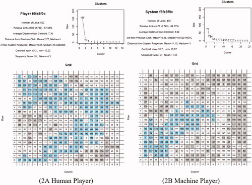
The next step was to average the trials per participant, human or machine, for import into SPSS 27, with two further R scripts. Two Excel sheets were generated with these R scripts, one for the human (transform5.r) and one for the machine players (transform6sys.r), see the OSF link above. We analyzed the eight largest place clusters and the longest sequence of places. We also generated a score of the average distance between all colored-in places of a player and of the average distance towards the next move.

Places were counted as belonging to a cluster when they had at least one side in common with another place of the same color. Places of the same color touching at the corners were not counted. Places were counted towards a sequence when (1) they were colored-in one after another and (2) they had one shared side with the consecutively colored-in place. For the longest sequence, it did not matter whether the consecutive place was added to the side, upwards, or downwards in direction as long as one side of two consecutive places had a shared boundary.

3. Results

The data OSF2021.sav are deposited on the Open Science Foundation (OSF) server. The sample was N = 522, consisting of 261 human participants and 261 machine players. We report the between-subject effects before the within-subject effects. Pairwise comparisons within the model were corrected by SPSS 27 according to Bonferroni, or manually by adjusting the p-level 0.05/number of comparisons. Effect sizes are partial effect sizes. When the Mauchly’s Test of Sphericity was significant, degrees of freedom were adjusted according to Greenhouse-Geisser and Epsilon is quoted. For pairwise comparisons, the standard errors of the means and the comparisons are reported.

We first ran an analysis of variance of the average reaction time of the humans in order to ascertain whether the speed instruction had been followed and was indeed the fastest in comparison. We then analysed the effect of the instructions on the four groups of human participants with respect to cluster size, and in another set of univariate analyses of variance the length and distribution of place sequences. Finally, the human-machine interaction was analysed with regards to these parameters.

3.1. The effect of instructions on human participants

3.1.1. Response time

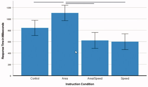
in this experiment was the average time participants took to color a place. For the human participants, a one-factorial 4 (instruction) ANOVA with response time as the dependent variable was conducted. The main effect of instruction, F(3, 261) = 11.43, p < 0.001, η_p² = 0.12, was significant. Pairwise comparisons within the model (Bonferroni) showed that the instruction to create an area made participants take more time (M = 1105 ms, SE 69.24), see Figure 3, compared to the control condition (M = 841 ms, SE 68.21), SE 97.19, p = 0.043, 95% CI [4.84, 521.70,], and the speed/area condition (M = 621 ms, SE 70.87), SE 99.08, p < 0.001, CI [220.33, 747.18] and the most time in comparison to the speed condition which was the fastest as expected (M = 599 ms, SE 70.31), SE 98.68, p < 0.001, CI [243.54, 768.29]. The two speed conditions did not differ from each other, p = 1.0. These results showed that participants were responsive to the specific task instructions.

Figure 3. Average time to color a place per instruction (n = 261, human players only). Note. The error bars denote the standard deviation. Horizontal bars indicate significant differences (please see the text for details).

3.1.2. Cluster size

A 8 (cluster) × 4 (instruction) mixed ANOVA with repeated measures of cluster size was conducted. The main effect of instruction, F(3, 261) = 7.50, p < 0.001, η_p² = 0.08, was significant. Pairwise comparisons within the model showed that all instructed conditions differed significantly from the control condition, p_s < 0.010, but not from each other, p_s = 1.0. All instructed conditions, with either time pressure or area instruction, yielded the same overall effect of the average area being about one to two places larger than in the standard instruction of the control group (M = 21.2, SE 0.26), that is, speed (M = 22.4, SE 0.27), SE 0.38, p = 0.010, CI [−2.21, −0.19], area (M = 22.8, SE 0.27), SE 0.38, p < 0.001, CI [−2.55, −0.55], and speed/area (M = 22.8, SE 0.27), SE 0.38, p < 0.001, CI [−2.53, −0.51].

Cluster size was significant as a main effect, F(1.09, 261) = 1809.32, p < 0.001, with a large effect size of η_p² = 0.88, and an epsilon of ε = 0.16, see Figure 4.

Figure 4. Cluster size (n = 261, human players only). Note. The error bars denote the standard deviation. All clusters differed significantly from each other, see the statistical values in Table A1.

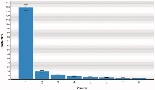
The cluster size (means with standard error in parentheses) varied from M = 134.74 (0.27) to M = 15.13 (0.82) to M = 8.93 (0.45) to M = 6.01 (0.28) to M = 4.62 (0.20) to M = 3.60 (0.16) to M = 2.98 (0.14) to M = 2.52 (0.12). Pairwise comparisons within the model demonstrated that the differences of all clusters were highly significant, p_s ≤ 0.001, see Table A1, showing that also the smaller cluster sizes all differed from each other. The decrease in cluster size is logical because the more places are colored-in and integrated into self-contained monochrome areas, the less space is left for the remaining clusters. This significant main effect of cluster size showed the strong spatial constraints that were generated by building a large area within the grid.

Important for the experimental hypothesis that the type of instruction would have an impact on cluster size was that the two-way interaction of cluster size and instruction was significant, F(21, 261) = 7.05, p < 0.001, η² = 0.08, see Figure 5.

Figure 5. Two-way interaction of instruction and cluster size (n = 261, human players only). Note. The error bars denote the standard error.

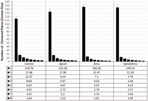
In Figure 5, all special instructions appear to yield a larger large cluster than the standard instruction. However, post-hoc univariate analyses, see Table A2, showed that for most cluster sizes, as hypothesized, only the area instructions (area and area/speed) yielded clusters that were significantly different to those of the control group. For the largest cluster, the explicit instruction to build an area was indeed conducive to build a larger area with a difference of about thirty places. Thereafter, the high spatial constraints induced by the large area caused the instruction to become ineffective for the second largest area (see Cluster 2 in Table A2). Moreover, for the smaller clusters, the explicit area instructions had the opposite effect, namely, the area instruction groups built smaller small areas than without such explicit instruction.

3.1.3. Place sequences

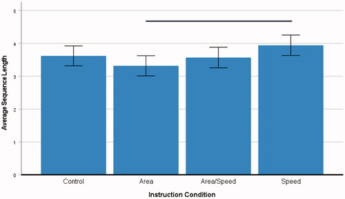
A one-factorial 4 (instructions) ANOVA was carried out with the average sequence length as the dependent variable. There was a significant main effect of instruction, F(3, 261) = 2.64, p = 0.050, η_p² = 0.03. Pairwise comparisons within the model showed that time pressure yielded significantly longer sequences (M = 3.94, SE 0.16) than the request to build an area (M = 3.32, SE 0.16), SE 0.22, p = 0.033, CI [0.03, 1.21], see Figure 6. However, the instruction showed no effect in another ANOVA with the maximal length of place sequences as dependent variable, p = 0.474.

Figure 6. Average sequence length per instruction (n = 261, human players only). Note. The error bars denote the standard deviation. The horizontal bar indicates a significant difference (please see the text for details).

The same analysis of variance with the variable measuring the average distance between places as dependent variable showed how much participants explored the spatial array with the 400 places. This analysis showed a main effect of instruction, F(1, 261) = 15.79, p < 0.001, η_p² = 0.16. Pairwise comparisons within the model showed that the standard instruction (M = 7.47, SE 0.06) yielded significantly larger distances than time pressure (M = 7.17, 0.06), SE 0.09, p = 0.003, CI [0.07, 0.53], area (M = 6.98, SE 0.06), SE 0.08, p < 0.001, [0.26, 0.71], or the area instruction combined with time pressure instruction (M = 6.94, SE 0.06), SE 0.09, p < 0.001, CI [0.30, 0.75], while there was no significant difference amongst the different instruction groups, p_s > 0.204.

The analysis of variance of the average distance of the next move showed how many places away coloring in one place would be from coloring-in the next place. Because sequencing of places would involve zero distance as they were directly adjacent to each other, we partialled out this variance by adding average sequence length as a covariate. The analysis confirmed the significance of the covariate, F(1, 261) = 164.30, p < 0.001, η_p² = 0.39, for controlling this analysis. A main effect of instruction, F(1, 261) = 5.70, p = 0.001, η_p² = 0.06, was found. Pairwise comparisons within the model showed that participants were more likely to color-in a further-away-place with the standard instruction condition (M = 3.61, SE 0.17) than under time pressure (M = 2.79, SE 0.18), SE 0.25, p = 0.006, CI [0.17, 1.48], and also when the time pressure instruction was combined with the request to create an area (M = 2.71, SE 0.17), SE 0.25, p = 0.002, CI [0.24, 1.55], while there was no difference to participants just instructed to build an area, (M = 3.20, SE 0.17), p = 0.595. This showed that time pressure hindered to explore the spatial array.

3.2. Human-machine interaction

In the following analyses of variance, we compare the human and the machine players with regards to the parameters area and sequencing vs. distance of places. We omitted the instruction factor for this purpose, because the machine was programmed to color-in places in a random fashion. A 8 (cluster) × 2 (human/machine) ANOVA with repeated measures of cluster size was conducted. There was a small main effect of the human-machine interaction, F(1, 522) = 29.78, p < 0.001, η_p² = 0.05, as humans were coloring-in on average slightly larger areas (M = 22.3) than the machine (M = 21.1).

Cluster size was significant as a main effect with a large effect size, F(1.15, 522) = 2319.89, p < 0.001, with a large effect size of η_p² = 0.82 and an Epsilon of ε = 0.16. The cluster size (means with standard error in parentheses) varied from M = 114.70 (SE 1.94) to M = 20.84 (SE 0.66) to M = 12.21 (SE 0.38) to M = 8.07 (SE 0.23) to M = 6.08 (SE 0.17) to M = 4.73 (SE 0.13) to M = 3.87 (SE 0.11) to M = 3.28 (SE 0.09). Pairwise comparisons within the model demonstrated again that the differences of all clusters were highly significant, p_s ≤ 0.001, see Table A3, showing that also the sizes of the smaller clusters all differed from each other. Importantly, there was a two-way interaction of cluster size with human vs. machine responses, F(7, 522) = 101.03, p < 0.001, η² = .16, see Figure 7.

Figure 7. Two-way interaction of cluster size in humans and the machine (N = 522). Note. The bars denote the standard error.

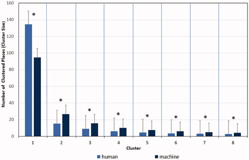
Post-hoc tests showed that human players built the largest area (M = 134.7, SE 2.77) significantly larger than the machine (M = 94.92, SE 2.70), while the machine built all the smaller clusters significantly larger than the human players, see the post-hoc tests in Table 1.

Table 1. Post-hoc t-tests (two-tailed, equal variances not assumed): human vs. machine cluster size (N = 522).

						95% CI of the difference
Cluster	t	df	p^a	M difference	SE	Lower	Upper
1	10.221	520.001	0.001	39.571	3.872	31.965	47.177
2	−8.591	496.176	0.001	−11.356	1.322	−13.953	−8.759
3	−8.632	484.181	0.001	−6.502	0.753	−7.982	−5.022
4	−8.712	491.866	0.001	−4.096	0.470	−5.019	−3.172
5	−8.480	493.876	0.001	−2.885	0.340	−3.554	−2.217
6	−8.472	495.287	0.001	−2.238	0.264	−2.756	−1.719
7	−8.026	502.563	0.001	−1.770	0.221	−2.203	−1.337
8	−7.931	504.386	0.001	−1.510	0.190	−1.884	−1.136

Note. ^aAdjustment for multiple comparisons: Bonferroni.

This result showed that the human players were able to build a larger area in the grid under low spatial constraints. However, under high spatial constraints caused by the largest cluster already occupying a great part of the matrix, more of a human advantage did not materialize. On the contrary, the system opponent built reliably larger small areas than humans in all of the remaining clusters.

3.2.1. Place sequences

A 2 (human/machine) mixed ANOVA was carried out with the maximal, longest sequence length as dependent variable. There was a significant difference between human and machine players, F(1, 522) = 294.78, p < 0.001, η_p² = 0.36. Clearly, the human players built sequences of places that were on average much longer (M = 14.54, SE 0.52) than those of the machine (M = 1.91, SE 0.52), see Figure 8, left.

Figure 8. Spatial relationships between places in human and machine (N = 522). Note. The bars denote the standard error.

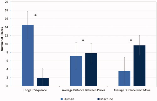
A second ANOVA with the variable measuring the average distance between places as dependent variable showed again a significant difference between human and machine player, F(1, 522) = 172.82, p < 0.001, η_p² = 0.25. The machine showed somewhat more distant colored-in places (M = 7.80, SE 0.03) than the human players (M = 7.14, SE 0.03), but the difference was not very large, see Figure 8, centre.

The ANOVA with average distance of the next move as dependent variable was run with average sequence length (sequences with zero distance) as control covariate. The significance of the covariate was confirmed, F(1, 522) = 125.65, p < 0.001, η_p² = 0.19. The significant difference between human players and the machine with a large effect size, F(1, 522) = 1816.55, p < 0.001, η_p² = 0.78, showed that the machine made moves that were more than double the distance (M = 9.70, SE 0.09) than the next moves that the human players made (M = 3.57, SE 0.09), see Figure 8, right.

3.3. Are place processing strategies and area building related?

In order to be sure that in human but not in machine players, the strategy of coloring-in consecutive places into a sequence rather than spatial exploration contributed to area building, correlations between maximal sequence length, average distance of the next move and cluster size were computed, see the correlation Table A4. The p-level of the correlations between the variables sequence length resp. average distance of the next move with the eight clusters were corrected per group (n = 261) according to Bonferroni, 0.05/16 = 0.003. There was no correction necessary for the human players as all correlations were p_s < 0.001. However, for the machine, while correlations were highly significant when considering the correlations between array exploration and clusters, only one correlation survived the Bonferroni adjustment of the correlations between sequence length and cluster size. In both players, smaller clusters were negatively correlated with the largest cluster, but positively with each other. Correlations between clusters were higher in the human players, but increased in the machine, the smaller the clusters were.

Figure 9 visualizes the direction (blue = negative, red = positive) and the size of the correlations (size of the circle) as well as the data points and slope of the distribution. Although the average distance of the next move was more pronounced in the machine than in the humans, in both players array exploration contributed significantly to the creation of areas. Array exploration was positively correlated with all clusters except the largest cluster where array exploration was negatively correlated. Thus, a similarity between human and machine players was that the largest area had the operational signs of the correlations reversed, pointing to its special status as a spatial constraint setter. A clear difference, though, was that in human players, sequence length showed a significant amount of shared variance with all clusters, but in the machine, this was not the case (column on the right).

Figure 9. Correlations between area, array exploration and place sequencing (N = 522). (A) Human players (n = 261). (B) Machine (n = 261).

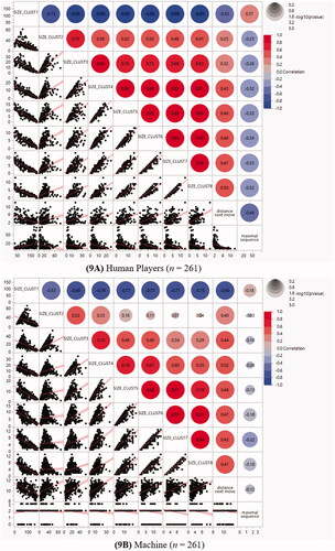
The next question was in which way distance of the next move (spatial array exploration) and the maximal length of the place sequences (pathways) could contribute to building areas. The second row from the bottom in Figure 9 visualizes the negative correlation of the largest cluster with spatial exploration as for both human players and the machine it was true that the larger the largest cluster, the less spatial exploration. Thus, to create the primary large area, in human players some inhibition of spatial exploration appears to occur. In contrast, the smaller clusters showed a positive correlation with spatial exploration as for both players, the larger the smaller clusters, the more spatial exploration had occurred. Hence, more exploration occurs when enlarging the smaller clusters.

In contrast to spatial exploration, the correlations of sequencing of places into pathways with the largest cluster size is positive, and the correlations with the smaller areas negative, that is, the direction of the correlations is the reverse, see the bottom row in Figure 9: The larger the primary cluster, the longer were the pathways that human players had lined up from consecutive places. In contrast, the larger their smaller clusters, the shorter was the pathway (see diminishing scale of the x-axes in the bottom row). The machine players did not create long pathways as they were limited to random spatial exploration and as a result only incidental sequences of about two places occurred. Still, despite the reduced variance of sequence length in the machine, the direction of the slopes showed that this result held true albeit with reduced correlations (see the exact p-values in Table A4).

4. Discussion

In development, humans make a transition from object-place units to regions that contain objects that have something in common (Lange-Küttner, 2006; Palmer, 1992). These regions were conceptualized by Lewin (1936) as zones within a spatial field. The spatial field here had a set number of square places and outer boundaries. There were no fixed barriers or dead ends like in a maze. Instead, as a challenge, the players encountered unpredictably and dynamically occurring occupations of places by the opponent. While the system had no choice but to randomly select an empty place, human players could decide to either color-in places randomly, or deploy a strategy. Thus, for the human players, the opponent could wreck their plans.

We have obtained several indicators that the human players were following an intentional strategy rather than coloring-in the places ad libitum like the machine. First, the human players were building a larger largest cluster than the machine. Second, they were sensitive to task instructions and could modify their strategy accordingly. When instructed to build an area, they built a bigger one. When set under time pressure, they colored in faster and only took time to build a smaller primary cluster from places. Third, the most compelling human strategy, though, was the sequencing of places into a pathway which could be seen as constituting a spatial heuristic to build areas. In contrast to the machine, adults colored-in long sequences of adjacent places, while the machine, with its random strategy, could only produce very short occasional place pairs. Due to the random strategy, the machine “explored” more of the array than humans, but correlations revealed that also humans used spatial exploration for building areas of clustered places.

Given the fundamental difference of this human-machine interaction with respect to building of pathways and spatial exploration, how could such a similarly structured spatial field be obtained? Theoretically, it would have been possible to create several same sized clusters by coloring-in adjacent places, or a chessboard pattern. Moreover, human players also did not imitate the random exploration of the game opponent. Instead, human players created sequences of places that significantly contributed to a large primary area. One cannot deny that such pathways leading towards an area have some similarity with the mathematical vectors that according to Lewin (1933) would give direction in a spatial field. But how could the machine build an equivalent area that was somewhat smaller yet similar in structure? The machine did not build randomly dispersed mid-size areas as could be expected given the random strategy. The reason would be that as the human players took the lead in creating one large area in the spatial field, the machine would consequently have the remaining space to itself. If the humans would not have embarked on building one large area, the machine would not have had the large empty swathe of the remaining space at its disposal to also build one large area, just by chance, without a concept (Lange-Küttner & Küttner, 2015). An area can emerge from randomly filled-in self-aggregating places, or is a result of intentionally planned areas (Lange-Küttner, 2009). However, usually these areas are planned with spatial axes or boundaries. This study is the first to show that pathways can lead to areas.

Interestingly, although the human players showed less spatial exploration than the machine, the correlations nevertheless proved that it still contributed to area building to about the same amount as for the machine player. The data visualizations showed that the primary large area was built with less spatial exploration. Thus, one could conclude that the human players did not explore the array with the clear intention to build one large area, as random spatial exploration could lead to the same result just by chance, as explained above. However, for the smaller areas this human area size-exploration rule was exactly the reverse: The larger the smaller clusters, the more spatial exploration. Thus, one can conclude that to build beyond the largest area, the human player had to make the next move further away. While the machine would do this anyway, the human players needed to expand their reach.

When it came to building pathways out of sequenced consecutive places, larger differences emerged between human and machine player. The machine could not build longer sequences as these only incidentally emerged and never became a sequence longer than two places. Hence, pathways only correlated with area size in the human players: Longer pathways contributed to the large primary cluster, but shorter pathways to smaller areas. Correlations were not larger than 0.37 so the areas were not completely built from pathways. Because of the large large-area:long pathway and large smaller-area:shorter pathway ratio it is likely that such pathways were created as area boundaries. Alternatively, they could have been built like spatial axes or vectors that could provide direction to the coloring-in activity, or if arranged in a shape, segment the array into zones. On the one hand, one could see it as a limitation that we did not make a difference between straight sequences and shaped sequences in this study, on the other hand, in studies like the one of Banino et al. (2018), the mazes also required to make turns, or going straight when approaching the pre-set goal.

In conclusion, an advantage of the grid game was that it was dynamic insofar as the pathways were made while walking (sequencing places). It was interactive insofar as the machine could frustrate plans. The restrictions on the machine player were programmed, while the human players could structure the array in any way they envisaged. Nevertheless, given the different degrees of freedom for the two players in this grid game, the results show that this unequal human-machine interaction followed the same logic of spatial constraints, pathways and spatial exploration when it comes to building spatial fields within a grid array.

Acknowledgments

I am grateful to the students at the University of Bremen (in alphabetic order) Harvn Bilici, Kira Detjen, Timon Dombrowski, Carina Feldle, Rae Kränzel, Alexandra Kurzywilk, Rachel Laftsidou, Marlene Lieder, Lea Nacken, Laura Sielemann, Sarah S. Siemsglüß, Tomke Tönjes and Sophie Walter for organizing the online data collection.

Disclosure statement

No potential conflict of interest was reported by the author(s).

Additional information

Notes on contributors

Christiane Lange-Küttner

Christiane Lange-Küttner is specialized in visual cognition. She studied at the Technical University Berlin. After her PhD at the Max Planck Institute of Human Development, she held posts at the Cognitive Science Lab, Free University Berlin, University of Aberdeen, London Metropolitan University, University of Konstanz, and the University of Greifswald.

Jörg Beringer

Jörg Beringer is specialized on usability and user experience. He obtained his PhD in Cognitive Psychology and Computer Science at the Technical University of Darmstadt, Germany. He developed the Experimental Run Time System (ERTS) scripting language that is used to run experiments and assessments on the Cognition Lab cloud platform.

Appendix

Table A1. Post-hoc tests of the cluster size (humans only, N = 261).

					95% CI for difference^a
Cluster	Cluster	M difference	SE	p^a	Lower bound	Upper bound
1	2	119.610	3.319	0.001	109.132	130.087
	3	125.810	3.059	0.001	116.154	135.466
	4	128.733	2.928	0.001	119.491	137.974
	5	130.120	2.859	0.001	121.095	139.144
	6	131.139	2.817	0.001	122.246	140.031
	7	131.764	2.793	0.001	122.948	140.580
	8	132.224	2.773	0.001	123.469	140.979
2	1	−119.610	3.319	0.001	−130.087	−109.132
	3	6.201	0.571	0.001	4.397	8.004
	4	9.123	0.697	0.001	6.921	11.325
	5	10.510	0.735	0.001	8.191	12.830
	6	11.529	0.753	0.001	9.151	13.908
	7	12.154	0.766	0.001	9.736	14.573
	8	12.615	0.781	0.001	10.150	15.079
3	1	−125.810	3.059	0.001	−135.466	−116.154
	2	−6.201	0.571	0.001	−8.004	−4.397
	4	2.922	0.262	0.001	2.095	3.750
	5	4.310	0.323	0.001	3.291	5.328
	6	5.329	0.351	0.001	4.219	6.438
	7	5.954	0.371	0.001	4.783	7.125
	8	6.414	0.386	0.001	5.196	7.632
4	1	−128.733	2.928	0.001	−137.974	−119.491
	2	−9.123	0.697	0.001	−11.325	−6.921
	3	−2.922	0.262	0.001	−3.750	−2.095
	5	1.387	0.125	0.001	0.994	1.781
	6	2.406	0.160	0.001	1.901	2.912
	7	3.031	0.182	0.001	2.456	3.607
	8	3.492	0.200	0.001	2.861	4.122
5	1	−130.120	2.859	0.001	−139.144	−121.095
	2	−10.510	0.735	0.001	−12.830	−8.191
	3	−4.310	0.323	0.001	−5.328	−3.291
	4	−1.387	0.125	0.001	−1.781	−0.994
	6	1.019	0.081	0.001	0.762	1.276
	7	1.644	0.106	0.001	1.308	1.980
	8	2.104	0.121	0.001	1.723	2.486
6	1	−131.139	2.817	0.001	−140.031	−122.246
	2	−11.529	0.753	0.001	−13.908	−9.151
	3	−5.329	0.351	0.001	−6.438	−4.219
	4	−2.406	0.160	0.001	−2.912	−1.901
	5	−1.019	0.081	0.001	−1.276	−0.762
	7	0.625	0.057	0.001	0.446	0.804
	8	1.085	0.078	0.001	0.839	1.332
7	1	−131.764	2.793	0.001	−140.580	−122.948
	2	−12.154	0.766	0.001	−14.573	−9.736
	3	−5.954	0.371	0.001	−7.125	−4.783
	4	−3.031	0.182	0.001	−3.607	−2.456
	5	−1.644	0.106	0.001	−1.980	−1.308
	6	−0.625	0.057	0.001	−0.804	−0.446
	8	0.460	0.047	0.001	0.312	0.608
8	1	−132.224	2.773	0.001	−140.979	−123.469
	2	−12.615	0.781	0.001	−15.079	−10.150
	3	−6.414	0.386	0.001	−7.632	−5.196
	4	−3.492	0.200	0.001	−4.122	−2.861
	5	−2.104	0.121	0.001	−2.486	−1.723
	6	−1.085	0.078	0.001	−1.332	−0.839
	7	−0.460	0.047	0.001	−0.608	−0.312

Note. Based on estimated marginal means. ^aAdjustment for multiple comparisons: Bonferroni.

Table A2. Post-hoc ANOVAs of the instruction effect on cluster size (n = 261) followed by pairwise comparisons within the model.

							95% CI of the difference
Cluster	F	df	p	M diff	SE	p^a	Lower bound	Upper bound
Cluster 1	7.54	3	0.001
C vs. S				−18.502	7.519	0.087	38.495	1.491
C vs. A				−31.584	7.461	0.001	51.421	−11.748
C vs. AS				−29.760	7.550	0.001	49.835	−9.686
S vs. A				−13.082	7.575	0.512	33.222	7.057
S vs. SA				−11.258	7.663	0.858	31.632	9.116
A vs. SA				1.824	7.605	1.001	18.396	22.044
Cluster 2	2.61	3	.052
C vs. S				0.598	2.303	1.001	−5.524	6.720
C vs. A				4.207	2.285	0.400	−1.867	10.281
C vs. AS				5.375	2.312	0.125	−0.772	11.522
S vs. A				3.608	2.319	0.726	−2.559	9.775
S vs. SA				4.777	2.346	0.257	−1.462	11.015
A vs. SA				1.168	2.329	1.001	−5.024	7.360
Cluster 3	4.49	3	0.004
C vs. S				2.314	1.254	0.396	−1.019	5.647
C vs. A				4.168	1.244	0.006	0.861	7.475
C vs. AS				3.677	1.259	0.023	0.330	7.024
S vs. A				1.853	1.263	0.861	−1.504	5.211
S vs. SA				1.363	1.277	1.001	−2.034	4.759
A vs. SA				−0.491	1.268	1.001	−3.862	2.880
Cluster 4	7.14	3	0.001
C vs. S				2.075	0.788	0.054	−0.021	4.172
C vs. A				3.484	0.782	0.001	1.404	5.563
C vs. AS				2.584	0.792	0.007	0.479	4.689
S vs. A				1.408	0.794	0.464	−0.703	3.520
S vs. SA				0.508	0.803	1.001	−1.628	2.645
A vs. SA				−0.900	0.797	1.001	−3.020	1.220
Cluster 5	6.74	3	0.001
C vs. S				1.358	0.575	0.114	−0.172	2.887
C vs. A				2.484	0.571	0.001	0.966	4.001
C vs. AS				1.791	0.578	0.013	0.256	3.327
S vs. A				1.126	0.579	0.318	−0.414	2.667
S vs. SA				0.434	0.586	1.001	−1.125	1.992
A vs. SA				−0.693	0.582	1.001	−2.240	0.854
Cluster 6	6.18	3	0.001
C vs. S				0.914	0.450	0.260	−0.282	2.110
C vs. A				1.844	0.446	0.001	0.658	3.031
C vs. AS				1.363	0.452	0.017	0.162	2.563
S vs. A				0.931	0.453	0.246	−0.274	2.136
S vs. SA				0.449	0.458	1.001	−0.770	1.668
A vs. SA				−0.482	0.455	1.001	−1.691	.728
Cluster 7	7.40	3	.001
C vs. S				0.709	0.382	0.388	−0.307	1.724
C vs. A				1.578	0.379	0.001	0.571	2.586
C vs. AS				1.451	0.384	0.001	0.432	2.471
S vs. A				0.870	0.385	0.148	−0.153	1.893
S vs. SA				0.743	0.389	0.345	−0.292	1.778
A vs. SA				−0.127	0.386	1.001	−1.154	0.900
Cluster 8	7.93	3	0.001
C vs. S				0.926	0.331	0.033	0.046	1.805
C vs. A				1.426	0.328	0.001	0.553	2.299
C vs. AS				1.346	0.332	0.001	0.463	2.229
S vs. A				0.500	0.333	0.806	−0.385	1.386
S vs. SA				0.420	0.337	1.001	−0.476	1.317
A vs. SA				−0.080	0.335	1.001	−0.970	0.809

Note. ^aAdjustment for multiple pairwise comparisons: Bonferroni. Instruction abbreviations are Control = C, Speed = S, Area = A, Area/Speed = AS. Significant comparisons are printed in bold.

Table A3. Post-hoc tests of the cluster size (humans/machine, N = 522).

					95% CI for difference^a
Cluster	Cluster	M difference	SE	p^a	Lower bound	Upper bound
1	2	93.854	2.401	0.001	86.314	101.395
	3	102.489	2.232	0.001	95.481	109.496
	4	106.623	2.132	0.001	99.929	113.316
	5	108.623	2.079	0.001	102.096	115.149
	6	109.969	2.046	0.001	103.546	116.393
	7	110.828	2.027	0.001	104.464	117.191
	8	111.418	2.012	0.001	105.099	117.737
2	1	−93.854	2.401	0.001	−101.395	−86.314
	3	8.634	0.526	0.001	6.982	10.286
	4	12.768	0.600	0.001	10.885	14.652
	5	14.768	0.628	0.001	12.795	16.741
	6	16.115	0.639	0.001	14.108	18.122
	7	16.973	0.644	0.001	14.950	18.996
	8	17.563	0.650	0.001	15.523	19.604
3	1	−102.489	2.232	0.001	−109.496	−95.481
	2	−8.634	0.526	0.001	−10.286	−6.982
	4	4.134	0.252	0.001	3.344	4.924
	5	6.134	0.309	0.001	5.164	7.104
	6	7.481	0.328	0.001	6.452	8.510
	7	8.339	0.339	0.001	7.274	9.404
	8	8.929	0.347	0.001	7.839	10.020
4	1	−106.623	2.132	0.001	−113.316	−99.929
	2	−12.768	0.600	0.001	−14.652	−10.885
	3	−4.134	0.252	0.001	−4.924	−3.344
	5	2.001	0.133	0.001	1.583	2.417
	6	3.347	0.161	0.001	2.842	3.852
	7	4.205	0.177	0.001	3.649	4.761
	8	4.795	0.187	0.001	4.206	5.384
5	1	−108.623	2.079	0.001	−115.149	−102.096
	2	−14.768	0.628	0.001	−16.741	−12.795
	3	−6.134	0.309	0.001	−7.104	−5.164
	4	−2.001	0.133	0.001	−2.417	−1.583
	6	1.347	0.078	0.001	1.103	1.591
	7	2.205	0.098	0.001	1.899	2.511
	8	2.795	0.109	0.001	2.454	3.136
6	1	−109.969	2.046	0.001	−116.393	−103.546
	2	−16.115	0.639	0.001	−18.122	−14.108
	3	−7.481	0.328	0.001	−8.510	−6.452
	4	−3.347	0.161	0.001	−3.852	−2.842
	5	−1.347	0.078	0.001	−1.591	−1.103
	7	0.858	0.052	0.001	0.696	1.020
	8	1.448	0.067	0.001	1.239	1.658
7	1	−110.828	2.027	0.001	−117.191	−104.464
	2	−16.973	0.644	0.001	−18.996	−14.950
	3	−8.339	0.339	0.001	−9.404	−7.274
	4	−4.205	0.177	0.001	−4.761	−3.649
	5	−2.205	0.098	0.001	−2.511	−1.899
	6	−0.858	0.052	0.001	−1.020	−0.696
	8	0.590	0.038	0.001	0.471	0.709
8	1	−111.418	2.012	0.001	−117.737	−105.099
	2	−17.563	0.650	0.001	−19.604	−15.523
	3	−8.929	0.347	0.001	−10.020	−7.839
	4	−4.795	0.187	0.001	−5.384	−4.206
	5	−2.795	0.109	0.001	−3.136	−2.454
	6	−1.448	0.067	0.001	−1.658	−1.239
	7	−0.590	0.038	0.001	−0.709	−0.471

Note. Based on estimated marginal means. ^aAdjustment for multiple comparisons: Bonferroni.

Table A4. Pearson correlations (two-tailed) between colored place distribution variables and area building (N = 522).

	Next	Length	1	2	3	4	5	6	7	8
Distance next move	1	−0.49**	−0.52**	0.25**	0.32**	0.43**	0.48**	0.48**	0.47**	0.50**
		0.001	0.001	0.001	0.001	0.001	0.001	0.001	0.001	0.001
Max. sequence length	−0.12	1	0.37**	−0.23**	−0.26**	−0.32**	−0.33**	−0.34**	−0.33**	−0.31**
	0.051		0.001	0.001	0.001	0.001	0.001	0.001	0.001	0.001
Cluster 1	−0.60**	0.18**	1	−0.73**	−0.85**	−0.90**	−0.90**	−0.90**	−0.88**	−0.85**
	0.001	0.004		0.001	0.001	0.001	0.001	0.001	0.001	0.001
Cluster 2	0.40**	−0.03	−0.53**	1	0.75**	0.58**	0.52**	0.50**	0.48**	0.41**
	0.001	0.608	0.001		0.001	0.001	0.001	0.001	0.001	0.001
Cluster 3	0.44**	−0.10	−0.68**	0.52**	1	0.84**	0.76**	0.72**	0.68**	0.63**
	0.001	0.099	0.001	0.001		0.001	0.001	0.001	0.001	0.001
Cluster 4	0.52**	−0.08	−0.76**	0.33**	0.70**	1	0.92**	0.88**	0.85**	0.81**
	0.001	0.176	0.001	0.001	0.001		0.001	0.001	0.001	0.001
Cluster 5	0.46**	−0.13*	−0.77**	0.18**	0.48**	0.78**	1	0.93**	0.89**	0.86**
	0.001	0.038	0.001	0.003	0.001	0.001		0.001	0.001	0.001
Cluster 6	0.47**	−0.18**	−0.77**	0.11	0.40**	0.67**	0.87**	1	0.94**	0.89**
	0.001	0.004	0.001	0.080	0.001	0.001	0.001		0.001	0.001
Cluster 7	0.42**	−0.22**	−0.76**	0.07	0.34**	0.60**	0.81**	0.91**	1	0.94**
	0.001	0.001	0.001	0.261	0.001	0.001	0.001	0.001		0.001
Cluster 8	0.40**	−0.18**	−0.75**	0.04	0.29**	0.55**	0.77**	0.87**	0.94**	1
	0.001	0.004	0.001	0.531	0.001	0.001	0.001	0.001	0.001

Note. Correlations for human participants are above the diagonal, for the machine system below the diagonal. **Correlation is significant at the 0.01 level (2-tailed). *Correlation is significant at the 0.05 level (2-tailed). Only Bonferroni-adjusted correlations are reported in the text.

References

- Anderson, M. D., Graf, E. W., Elder, J. H., Ehinger, K. A., & Adams, W. J. (2021). Category systems for real-world scenes. Journal of Vision, 21(2), 8–8. https://doi.org/10.1167/jov.21.2.8
- Banino, A., Barry, C., Uria, B., Blundell, C., Lillicrap, T., Mirowski, P., Pritzel, A., Chadwick, M. J., Degris, T., Modayil, J., Wayne, G., Soyer, H., Viola, F., Zhang, B., Goroshin, R., Rabinowitz, N., Pascanu, R., Beattie, C., Petersen, S., … Kumaran, D. (2018). Vector-based navigation using grid-like representations in artificial agents [Neural Networks 4160]. Nature, 557(7705), 429–433. https://doi.org/10.1038/s41586-018-0102-6
- Bar-Hillel, M., & Wagenaar, W. A. (1991). The perception of randomness. Advances in Applied Mathematics, 12(4), 428–454. https://doi.org/10.1016/0196-8858(91)90029-I
- Bhargav, B., Dinesh, H., & Mahapatra, I. B. (2019). Methodologies in augmented reality. International Research Journal of Engineering and Technology, 6(3), 1536–1542. https://www.irjet.net/archives/V6/i3/IRJET-V6I3289.pdf.
- Biederman, I. (1987). Recognition-by-components: A theory of human image understanding. Psychological Review, 94(2), 115–147. https://doi.org/10.1037/0033-295X.94.2.115
- Biederman, I. (2000). Recognizing depth-rotated objects: A review of recent research and theory. Spatial Vision, 13(2–3), 241–253. https://doi.org/10.1163/156856800741063
- Brugger, P., Monsch, A. U., Salmon, D. P., & Butters, N. (1996). Random number generation in dementia of the Alzheimer type: A test of frontal executive functions. Neuropsychologia, 34(2), 97–103. https://doi.org/10.1016/0028-3932(95)00066-6
- Ehinger, K. A., & Wolfe, J. M. (2016). When is it time to move to the next map? Optimal foraging in guided visual search. Attention, Perception & Psychophysics, 78(7), 2135–2151. https://doi.org/10.3758/s13414-016-1128-1
- Faul, F., Erdfelder, E., Lang, A.-G., & Buchner, A. (2007). G*Power 3: A flexible statistical power analysis program for the social, behavioral, and biomedical sciences. Behavior Research Methods, 39(2), 175–191. https://doi.org/10.3758/BF03193146
- Gobet, F., De Voogt, A., & Retschitzki, J. (2004). Moves in mind. The psychology of board games. Psychology Press.
- Julesz, B. (1971). Foundations of cyclopean perception. University of Chicago Press.
- Krupic, J., Bauza, M., Burton, S., & O'Keefe, J. (2016). Framing the grid: effect of boundaries on grid cells and navigation. The Journal of Physiology, 594(22), 6489–6499. https://doi.org/10.1113/JP270607
- Kubovy, M., & Gilden, D. (1991). Apparent randomness is not always the complement of apparent order. In G. R. Lockhead & J. R. Pomerantz (Eds.), The perception of structure: Essays in honor of Wendell R. Garner (pp. 115–127). American Psychological Association. https://doi.org/10.1037/10101-006
- Lange-Küttner, C. (1997). Development of size modification of human figure drawings in spatial axes systems of varying complexity. Journal of Experimental Child Psychology, 66(2), 264–278. https://doi.org/10.1006/jecp.1997.2386
- Lange-Küttner, C. (2004). More evidence on size modification in spatial axes systems of varying complexity. Journal of Experimental Child Psychology, 88(2), 171–192. https://doi.org/10.1016/j.jecp.2004.02.003
- Lange-Küttner, C. (2006). Drawing boundaries: From individual to common region – the development of spatial region attribution in children. British Journal of Developmental Psychology, 24, 419–427. https://doi.org/10.1348/026151005X50753
- Lange-Küttner, C. (2009). Habitual size and projective size: The logic of spatial systems in children’s drawings. Developmental Psychology, 45(4), 913–927. https://doi.org/10.1037/a0016133
- Lange-Küttner, C. (2013). Array effects, spatial concepts, or information processing speed: What is the crucial variable for place learning? Swiss Journal of Psychology, 72(4), 197–217. https://doi.org/10.1024/1421-0185/a000113
- Lange-Küttner, C., & Beringer, J. (2022). Spatial heuristics in the grid game: Children, adults and the machine coloring-in places Manuscript under review.
- Lange-Küttner, C., & Küttner, E. (2015). How to learn places without spatial concepts: Does the what-and-where reaction time system in children regulate learning during stimulus repetition? Brain and Cognition, 97, 59–73. https://doi.org/10.1016/j.bandc.2015.04.008
- Lange-Küttner, C., & Puiu, A.-A. (2021). Perceptual load and sex-specific personality traits. Experimental Psychology, 68(3), 149–164. https://doi.org/10.1027/1618-3169/a000520
- Lewin, K. (1933). Vectors, cognitive processes, and Mr. Tolman's criticism. Journal of General Psychology, 8(2), 318–345. https://doi.org/10.1080/00221309.1933.9713191
- Lewin, K. (1936). Principles of topological psychology. Reprint 2013 by Read Books Ltd.
- Marr, D., Hildreth, E., & Brenner, S. (1980). Theory of edge detection. Proceedings of the Royal Society of London. Series B, Biological Sciences, 207(1167), 187–217. https://doi.org/10.1098/rspb.1980.0020
- Nash, J. (1951). Non-cooperative games. The Annals of Mathematics, 54(2), 286–295. https://doi.org/10.2307/1969529
- Palmer, S. E. (1992). Common region: A new principle of perceptual grouping. Cognitive Psychology, 24(3), 436–447. https://doi.org/10.1016/0010-0285(92)90014-S
- Silver, D., Huang, A., Maddison, C. J., Guez, A., Sifre, L., van den Driessche, G., Schrittwieser, J., Antonoglou, I., Panneershelvam, V., Lanctot, M., Dieleman, S., Grewe, D., Nham, J., Kalchbrenner, N., Sutskever, I., Lillicrap, T., Leach, M., Kavukcuoglu, K., Graepel, T., & Hassabis, D. (2016). Mastering the game of Go with deep neural networks and tree search. Nature, 529(7587), 484–489. https://doi.org/10.1038/nature16961
- Szentandrási, I., Herout, A., & Dubská, M. (2012). Fast detection and recognition of QR codes in high-resolution images [Paper presentation]. Proceedings of the 28th Spring Conference on Computer Graphics, Budmerice, Slovakia. https://doi.org/10.1145/2448531.2448548
- Tolman, E. C, (1948). Cognitive maps in rats and men. Psychological Review, 55(4), 189–208. https://doi.org/10.1037/h0061626
- Towse, J. N., & McLachlan, A. (1999). An exploration of random generation among children. British Journal of Developmental Psychology, 17(3), 363–380. https://doi.org/10.1348/026151099165348
- Towse, J. N., & Neil, D. (1998). Analyzing human random generation behavior: A review of methods used and a computer program for describing performance. Behavior Research Methods, Instruments, & Computers, 30(4), 583–591. https://doi.org/10.3758/BF03209475
- Treisman, M., & Faulkner, A. (1987). Generation of random sequences by human subjects: Cognitive operations or psychological process? Journal of Experimental Psychology: General, 116(4), 337–355. https://doi.org/10.1037/0096-3445.116.4.337
- Turing, A. M. (1950). Computing machinery and intelligence. Mind, LIX(236), 433–460. https://doi.org/10.1093/mind/LIX.236.433