Evolutionary Algorithm for Vehicle Driving Cycle Generation

ABSTRACT

Modeling transit bus emissions and fuel economy requires a large amount of experimental data over wide ranges of operational conditions. Chassis dynamometer tests are typically performed using representative driving cycles defined based on vehicle instantaneous speed as sequences of “microtrips”, which are intervals between consecutive vehicle stops. Overall significant parameters of the driving cycle, such as average speed, stops per mile, kinetic intensity, and others, are used as independent variables in the modeling process. Performing tests at all the necessary combinations of parameters is expensive and time consuming. In this paper, a methodology is proposed for building driving cycles at prescribed independent variable values using experimental data through the concatenation of “microtrips” isolated from a limited number of standard chassis dynamometer test cycles. The selection of the adequate “microtrips” is achieved through a customized evolutionary algorithm. The genetic representation uses microtrip definitions as genes. Specific mutation, crossover, and karyotype alteration operators have been defined. The Roulette-Wheel selection technique with elitist strategy drives the optimization process, which consists of minimizing the errors to desired overall cycle parameters. This utility is part of the Integrated Bus Information System developed at West Virginia University.

IMPLICATIONS

It is expected that the paper will provide a useful tool for modeling and analysis of vehicle fuel economy and emissions and for the design, optimization, and analysis of driving cycles for testing and vehicle fleet management.

INTRODUCTION

In recent years, automotive pollution has become a major societal issue. Large efforts have been focused on designing lower-emission vehicles with increased fuel economy. In this context, modeling combustion engine emissions and fuel economy to provide prediction and analysis tools has received considerable attention from the research community, primarily under the auspices of the United States Environmental Protection Agency1–3 (EPA).

The Integrated Bus Information System (IBIS) is a vehicle fleet emission and fuel economy prediction software, currently under development at West Virginia University (WVU). The overall goal of IBIS is to provide an interactive, approachable, and reliable method for users—primarily transit agencies—to evaluate overall fleet emissions and fuel consumption and to optimize fleet configuration and operation. The modeling strategy for IBIS is based on the WVU Center for Alternative Fuels, Engines, and Emissions (CAFEE) vehicle emission database. Multiple variable polynomials created through linear regression produce estimates of fuel economy, and of emissions of carbon dioxide, carbon monoxide, oxides of nitrogen, hydrocarbons, and particulate matter. The independent variables are average speed with idle, stops per mile, percentage idle, standard deviation of speed with idle, and kinetic intensity,4 defined as the ratio of the characteristic acceleration and the square of aerodynamic speed. These five parameters were selected to be used for modeling based on a correlation study of duty cycle parameters' effects on fuel economy and emissions.4 Distinct models, referred to as “backbone models”, have been produced for transit vehicles using conventional diesel, compressed natural gas (CNG), and diesel-electric hybrid architectures. Additionally, multiplicative and additive correction factors are computed and applied to these backbone models to account for variances in vehicle configurations and technologies.

The CAFEE emission database consists of second-by-second data for a variety of standard driving cycles performed on vehicles of different configurations over a period of more than two decades. For accurate modeling, large amounts of data, adequately distributed over the entire range of the independent variables, are necessary. Typically this condition is not met and substantial gaps in the available data exist. Performing additional tests to fill in these gaps is costly and time consuming. In this paper, an alternative solution is proposed based on the fact that standard driving cycles are sequences of microtrips, which are periods of nonidle operation. These segments can be isolated from within available tests, rearranged, and concatenated such that “new” driving cycles are generated that exhibit the required values of the independent variable (e.g., average speed or stops per mile) to fill in the gaps in the regression data. It is critical that the variation in the fuel economy and emissions of the microtrips with respect to their relative location within the cycle is minimal. To ensure this hypothesis, all test vehicles have been warmed up prior to data collection and the aftertreatment devices were kept within their operational temperatures. The effects on the emissions of the immediate cycle history leading up to a microtrip were limited and the characteristics of the newly generated cycles followed the trends of the experimental data. Concatenation of microtrips has been previously used only to build statistically representative cycles to match experimental databases.5,6

The development of a computational tool based on genetic or evolutionary algorithms (EAs) for driving cycle generation within an interactive integrated design environment7 in MATLAB/Simulink is presented in this paper. A brief review of the main general aspects of the evolutionary or genetic algorithms is presented and the problem of generating new driving cycles via microtrips concatenation using EAs is formulated. The general architecture of the EA and its component modules are discussed in detail. The graphical user interface and the options available for the driving cycle generation are described. The functionality of the design tool is illustrated through some examples. Finally, the main conclusions are summarized.

THE EVOLUTIONARY PARADIGM FOR SOLUTION SEARCH AND OPTIMIZATION

In the biological world, organisms must struggle for survival. These individuals may undergo random changes in their genetic makeup, which can alter their structural and functional characteristics (genotype and phenotype, respectively). When these changes are beneficial to the organism, it is better equipped to adapt and survive environmental conditions. As a result, the individual will live longer and will have a better chance of reproducing and transferring its genes to subsequent generations. Therefore, there will be a higher probability of these genes being present in future populations. After several generations, it is expected that the new “good” genes will dominate the population. This optimum is, however, temporary, because the environmental conditions are typically in a permanent state of change.

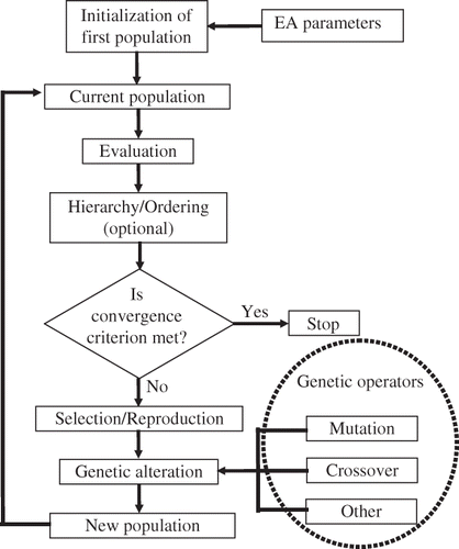
EAs are parameter iterative search techniques that rely on analogies to natural biological processes.8,9 This class of artificial intelligence techniques simulates the evolution of species and individual selection based on Darwin's “survival of the fittest” principle to perform parameter optimization. EAs work simultaneously on a set (population) of potential solutions (individuals) to the problem under investigation. Within the EA paradigm, individuals are also referred to as “chromosomes”. For the purpose of generating a driving cycle with prescribed global characteristics, an individual will consist of a sequence of microtrips. A set of design requirements and constraints must be defined, which play the role of the environment. They can be expressed mathematically, logically (binary or fuzzy), or in a descriptive manner; they can also be totally independent from one another. This capability is one of the most important properties of EAs. The degree to which solutions meet the performance requirements and constraints is evaluated and used to select “surviving” individuals that will “reproduce” and generate a new population. Individuals will now undergo alterations similar to the natural genetic mutation and crossover and possibly other genetic operators. The next iteration starts with this new population (new set of possible solutions). The process continues until there is no longer a significant increase in the performance of the best solution and/or the maximum number of iterations setup by the user is reached. The block diagram of a typical EA is presented in Figure 1.

Figure 1. Block diagram of an evolutionary algorithm.

EAs rely on two processes that are contradictory to some extent: exploration and exploitation. “Exploration” is the process of browsing the solution space in search of “better” solutions and “exploitation” is the process of tuning a “good” solution through searching within its vicinity. The various parameters of the EA (size of the population, genetic alteration rates, selection method) have a decisive impact on the balance between “exploration” and “exploitation” and hence on the performance of the algorithm. For example, a population that has too few individuals may not allow the EA to explore enough of the solution space. This may result in poor convergence, long search duration, and/or convergence to a local extremum. If the population is too large, the duration to compute an iteration could be excessive and, hence, make a complete successful search process unreachable. An EA can converge prematurely to a local extremum if a solution/individual that is much “better” than most of the others in the population emerges early on in the process and there is too much emphasis on exploitation. It may reproduce so abundantly that it drives down the population's diversity too soon. Such phenomena can be avoided by careful selection of the EA parameters.

Optimization has become a major field of EA applicability. As compared to the widely used gradient methods and enumerative schemes, EAs are global and robust over a broad spectrum of problems.10 EAs have shown excellent potential for solving highly complex nonlinear parameter optimization problems. In general, the advantages of using EAs include

•	Parallelism. The gradient-based methods are capable of searching for the solution in one direction at a time. If the algorithm does not converge or a local suboptimum is reached the search must be reinitiated. The EAs perform the search in multiple directions due to the fitness-based selection and the randomness of the changes from one generation to the next.
•	Complexity of performance criteria. The performance criteria (or fitness) do not have to be expressed as an analytical function. There are no requirements for continuity, derivability, or bijectivity. The formulation of the constraints can be arbitrary.
•	Globality. If properly designed by selecting EA parameters that establish an adequate balance between exploration and exploitation, EAs can escape the trap of local extrema and given enough iterations they will reach the global extremum.
•	Dimensionality. The EAs are capable of efficiently handling problems with huge numbers of parameters and objectives (and/or constraints).
•	Generality. EAs are not necessarily dependent on the problem they are supposed to solve. They do not have to use previously known domain-specific information. This lack of preconceptions allows the EAs to investigate all possible search pathways and possibly search through regions excluded by more conventional algorithms. However, domain specific information can be used to constrain the search and avoid wasting computational time in regions that are not expected to lead to the solution.

PROBLEM FORMULATION

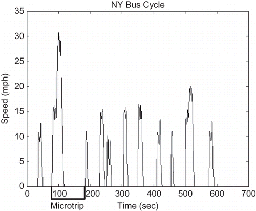
Within the IBIS development strategy, the models of emissions and fuel economy consist of polynomials determined through linear regression and based on five independent variables. Experimental data uniformly distributed throughout this five-dimensional hyperspace are necessary for adequate model development. One point in this independent variable hyperspace corresponds to one particular driving cycle. It would be extremely costly and time consuming to perform such an exhaustive testing program. Considering that standard test driving cycles consist of series of segments or microtrips defined as periods between consecutive idles, it is possible to create new cycles by combining segments of data from existing second-by-second experimental data. Figure 2 presents an example of a microtrip defined within the New York City bus cycle (NYBUS). Second-by-second emissions and fuel consumption data can be isolated for each microtrip from available tests. These microtrips can be combined and duplicated to obtain the desired overall characteristics of the new cycle.

Figure 2. Microtrip definition in the NY bus cycle.

The problem of filling in the gaps in the test data to be used in the regression algorithm is equivalent to finding a set of microtrips whose overall cycle characteristics expressed in terms of the five independent modeling variables are as close as possible to the specific points of the gaps. Due to the lack of an analytical formulation, high dimensionality, and nonlinearity of this optimization problem, evolutionary algorithms are expected to provide the most effective tools. It should be noted that the proposed method does not depend on the number or nature of the independent variables used for modeling.

A microtrip database was created using trips from 12 standard cycles. The measured second-by-second emissions data were first time-aligned with vehicle speed (corrected for measurement delay), then the cycles were broken into microtrips.

A potential solution to the problem, hence an individual or chromosome, is a set of microtrips including duplicates or not. The size of this set may vary. It should be noted that the order of the microtrips is not relevant for the overall characteristics of the cycle. At all times during the optimization process, the microtrips belong to the microtrip database for which second-by-second measurements are available.

DESCRIPTION OF THE EVOLUTIONARY ALGORITHM MODULES

Representation of the Individual

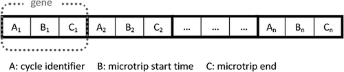
The individual or chromosome consists of a variable number of genes, each gene corresponding to a microtrip. The order of the genes within the chromosome is tracked only for the execution of the various algorithms and is not important for the overall characteristics of the new cycles. A gene is a three-integer structure; however, this implementation can be categorized as using the real representation. The first integer is an index marker pertaining to 1 of the 12 standard test cycles, and the subsequent integers are time markers for the respective beginning and end of a microtrip within the given cycle. The general structure of an individual is illustrated in Figure 3. The number of genes, n, may vary from individual to individual and can also be changed during the reproduction phase as a result of genetic alteration. This structure of the microtrip representation was chosen because it lends the newly created cycles to more flexibility. This flexibility occurs because new second-by-second emission data do not need to be modified, excepting time alignment, because the model references time bands within a given standard cycle. This proved useful when moving between vehicle configurations and fuel types, given that the emission data are represented in 1 or more of the 12 cycles.

Figure 3. Structure of an individual (real representation).

Initial Population

The number of individuals in the population is an important EA design parameter that must be set correctly to ensure sufficient coverage of the search space and variability within the population. The initial population is created by randomly selecting microtrips and aligning them into individuals of a predefined length. The size of the chromosome may vary from one iteration to the next and from individual to individual. However, a maximum limit is imposed for practical purposes. The size of the population has been kept constant within this implementation.

Performance Index

Through the concatenation of microtrips, each individual represents a new cycle. The objective is to obtain new cycles that achieve desired overall values of one, several, or all of the independent variables (IVs) used for modeling (average speed with idle, standard deviation of speed with idle, stops per mile, percentage idle, and kinetic intensity). First, a relative error e is computed for each IV using the relationship:

(1)

where is the desired value of the cycle parameter and is the corresponding value determined for the new cycle (individual). An evaluation index is computed next:

(2)

where is a user-defined maximum relative error. Finally, the performance index (PI) for the individual is calculated as a weighted average of the evaluation indexes for all IVs of interest:

(3)

where w are weight factors defined by the user and is the number of IVs imposed for the generation of the new cycle. In this paper, . The weights affecting the IVs determine the characteristics of the newly generated cycle and are not related to the impact of the IVs as modeling parameters. The evaluation process is repeated for each individual in the population to determine their “fitness”. Note that “better” individuals will have higher PI.

Selection and Reproduction

Once each individual has been evaluated, they are selected to reproduce based on their PI. Individuals with higher PI will get more chances to produce “offspring”, in other words, there will be more copies of themselves in the next generation. In this implementation, the Roulette-Wheel selection method augmented with the elitist strategy has been used.8,9 The first step of the Roulette-Wheel selection method consists of computing the total fitness of the population, TF, as the sum of the performance indexes of all individuals in the current population/generation:

(4)

Next, the probability of selection p for each individual is computed:

(5)

Then the cumulative probability q is calculated for each individual as follows:

(6)

Finally, the roulette wheel is “spun” by generating random numbers . The preliminary new population is determined by selecting individuals from the parent generation based on their corresponding and cumulative probability . For each of the available spots in the new population (note that the size of the population is kept constant through generations), the following condition is checked with respect to the parent population:

(7)

The parent individual for which condition 7 is satisfied will fill in the available spot in the new population. Individuals with higher performance indices will get larger cumulative probability intervals and more chances for multiple copies in the new generation.

The elitist selection is a strategy that allows the best individual to survive unaltered from one generation to the next. The best individual of the current generation is simply introduced into the next. This ensures that good solutions obtained at different moments during the EA are not lost without finding a better one, thus emphasizing exploitation and accelerating convergence.

Genetic Operators

Three distinct genetic operators (GOs)—mutation, crossover, and karyotype alteration—are performed on the population according to GO rates established by the designer. The individuals that are subject to genetic alteration are selected randomly.

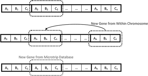
The mutation GO was designed with the intention to produce small alterations of the individuals, in an effort to focus the search in the vicinity of existing solutions. The alteration consists of replacing a gene (microtrip) with a different one from within the individual, or with a new one from the microtrip database. Both types of mutation are illustrated in Figure 4. The gene subject to mutation, the replacing gene, and its source are all selected randomly. Both type of mutation have equal probability of occurrence.

Figure 4. Gene mutation.

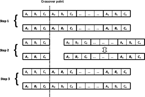
The crossover GO can be viewed as a mimicry of the biological crossover process where segments of genetic material are swapped between chromosomes. It can also be interpreted as similar to the sexuate reproduction, where offspring inherit part of their genetic material from one parent and part from the other. Pairs of individuals are randomly selected to undergo crossover. First, they are evaluated in length and the larger of the two has a crossover point randomly selected between two genes. The genes from the larger are combined with the smaller using the genes up to the crossover point from the larger individual and the genes from the crossover point of the smaller individual, and vice versa. This results in two new individuals consisting of parts of the parent pair, as presented in Figure 5.

Figure 5. Single point crossover.

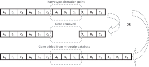
The karyotype represents the set of main structural characteristics of the genetic material of a species. It includes the number of chromosomes, their shape, gene topology, and other physical properties. Within this EA, karyotype alteration consists of adding a gene to or removing a gene from a randomly selected location within the chromosome. The individual to be subject to karyotype alteration is selected randomly according to the alteration rate, which governs the likelihood that a chromosome will change in length. Gene addition and deletion have equal probability of occurring. The gene to be added is selected randomly from the entire microtrip database. In the extreme case of an individual comprised of only one gene (microtrip), the microtrip will be replaced with a new microtrip rather than deleted. Figure 6 presents the schematic of this GO.

Figure 6. Karyotype alteration—addition or removal of genes.

Convergence Criterion

The new population is completely defined after the GOs are applied as many times as dictated by the genetic alteration rates. The new generation will now be subject to the same process as the parent population. No formal convergence criterion is used in this implementation. Instead, the cycle is repeated for a prespecified number of iterations. The computational tool has the capability to restart the genetic search using a prerecorded initial population, which may be the result of a previous search. In this way, if at the end of the prespecified number of iterations the solution is not satisfactory, the search can be continued for another number of iterations.

DESCRIPTION OF THE INTERACTIVE UTILITY FOR DRIVING CYCLE GENERATION

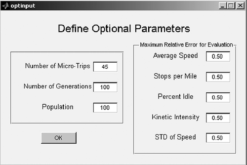
The computational tool for interactive cycle generation is developed in MATLAB/Simulink and relies on an advanced user-friendly graphical interface to allow design flexibility and effectiveness. The main menu presented in Figure 7 allows users to define the target driving parameters for the output cycle, as well as the relative importance of each parameter by setting its weight. A weight value of 0 means that the parameter must not be considered as part of the performance index and any value arbitrarily resulting from the cycle building process is acceptable. Additionally, the user can modify the default parameters regarding the number of iterations, size of the initial population, maximum length of initial chromosomes (in terms of number of microtrips), and the maximum relative errors for each input parameter. These actions can be performed using the menu presented in Figure 8.

Figure 7. Cycle generator interface.

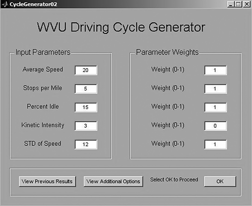
Figure 8. EA design parameters.

Once the user initializes the tool, the rates for mutation, crossover, and karyotype alteration are set to default values that were determined to achieve a good balance between exploration and exploitation. If desired or needed, the alteration rates can be changed in the MATLAB script, which includes ample comments to facilitate such an action.

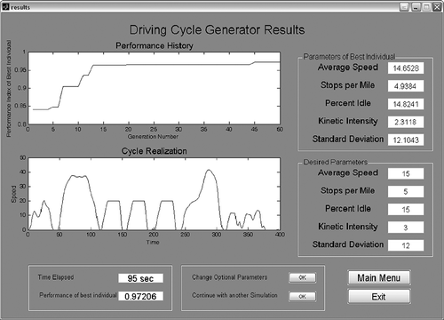
Upon conclusion of the simulation, the user is presented with a results window. This window shows the performance history with each generation and a graphical realization of the newly created cycle. Additionally the user is presented with the values of the target parameters and the actual parameters of the newly created cycle. At this point, the user can change the optional parameters and rerun the tool, or they can continue with the simulation with the last population (i.e., add more generations). This is particularly useful when the user does not receive results that are satisfactory, or when they are unable to run large numbers of iterations due to computational or scheduling constraints. Figure 9 shows an example results window.

Figure 9. Example results window from the EA computational tool.

EXAMPLE RESULTS USING THE EA FOR DRIVING CYCLE GENERATION

In this section, the process of creating new driving cycles using the cycle generator computational tool is described. The cycle created in this example was expected to achieve an average speed of 15 mph, 5 stops per mile, 15% idle, and a standard deviation of speed of 12 mph. Kinetic intensity is to be omitted (arbitrarily) from this example. This means that any overall cycle value for this parameter is acceptable and the parameter is removed from the performance evaluation. All other four modeling parameters are considered to be equally important. Therefore, the weight corresponding to the kinetic intensity is set to 0 whereas all others are 1. These parameters are entered through the interface presented in Figure 7.

The general parameters required for the EA are entered using the interface presented in Figure 8. In this example, the maximum number of microtrips in a cycle is set to 45, the population consists of 100 individuals, and the algorithm will stop after 50 iterations.

The results for this example (Figure 9) show that the tool is able to create a cycle with a performance index of approximately 0.97 on a scale from 0 to 1 with a computational time of 95 sec. In addition to the values of each parameter, the results window displays a realization of the cycle. This is helpful in determining whether or not the cycle that was created is a practical cycle.

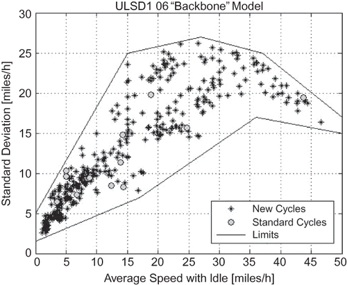
Given the full possible range of each of the five modeling parameters, a 5-dimensional hyper-rectangle can be defined, which includes all possible combinations of the parameters. However, not all these combinations are physically/technically possible. The EA-based cycle generator can be used to define the regions of the modeling parameters hyper-rectangle that are physically possible, within the limitations of the microtrip database. Such information is valuable for analysis and modeling. Acceptable limits for four modeling parameters in terms of average speed have been determined within the IBIS project in this way. The limits for kinetic intensity, percentage idle, stops per mile, and speed standard deviation as functions of average speed with idle are presented in Figures 10 through 13, respectively.

Figure 10. Limits on kinetic intensity as function of average speed.

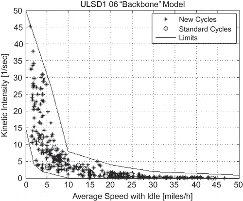
Figure 11. Limits on percentage idle as function of average speed.

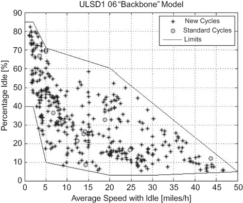
Figure 12. Limits on stops per mile as function of average speed.

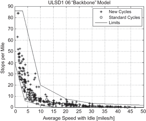
Figure 13. Limits on speed standard deviation as function of average speed.

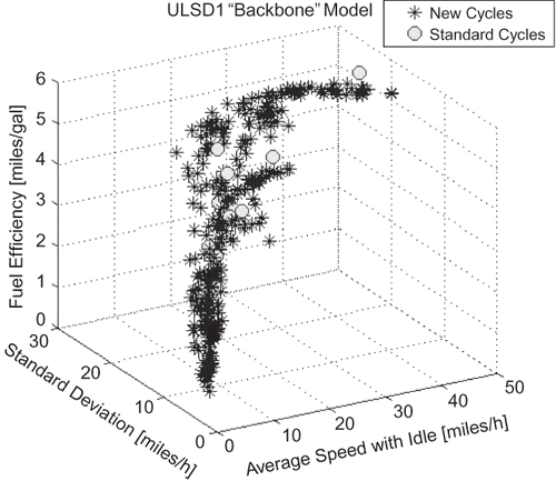
In Figure 14, the fuel efficiency as a function of average speed and speed standard deviation is presented for generated cycles for a 2000 model year diesel-fueled transit bus. Note that this is a three-dimensional cross-section of the previously described five-dimensional domain of the independent modeling variables. For comparison, the values of the 12 experimental standard cycled are presented on the same axes system. It can be seen that the points cover the domain adequately for regression-based modeling.

Figure 14. Fuel efficiency of generated cycles.

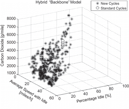
Another example is shown in Figure 15. The carbon dioxide emissions of the generated and initial driving cycles are plotted versus average speed with idle and percentage idle as independent variables. In this case, data from a 2006 diesel-fueled bus with a hybrid architecture are used. A uniform coverage of the domain is achieved with the generated cycles.

Figure 15. Carbon dioxide emissions of generated cycles.

CONCLUSIONS

A methodology was presented for obtaining new regression points for transit bus emission and fuel efficiency modeling from experimental data. Segments (microtrips) of standard test driving cycles are recombined to obtain new cycles with desired overall cycle parameters. The approach can potentially reduce significantly the time and cost of experiments.

An advanced computational tool for driving cycle generation has been developed in MATLAB relying on an evolutionary algorithm with customized components in terms of genetic representation and genetic operators. The genetic search was proved to be an effective and efficient tool for this problem.

The proposed algorithm is capable of defining new driving cycles with specified parameters with reduced experimental data preprocessing and low computational time. The newly defined cycles can be used to support modeling vehicle emissions and fuel efficiency, analyzing the effects of various driving factors on vehicle emissions and fuel efficiency, and designing experimental tests.

ACKNOWLEDGMENTS

This research effort was sponsored by the Federal Transit Administration through grant WV-26-7008.

REFERENCES

- U.S. Environmental Protection Agency . Mobile Source Emission Factor Model—User Guide . EPA420-R-03-010 . 2003 . U.S. Government Printing Office: Washington, DC
- U.S. Environmental Protection Agency; Nam, E . Advanced Technology Vehicle Modeling in PERE . EPA420-D-04-002 . 2004 . U.S. Government Printing Office: Washington, DC
- U.S. Environmental Protection Agency , Glover , E. , Koupal , J. , Cumberworth , M. , Brzezinski , D. , Shyu , G. , Gianelli , B. , Landman , L. , Beardsley , M. , Warila , J. , Nam , E. , Michaels , H. , Hart , C. , Srivastava , S. and Tierney , G. MOVES2004 User Guide . EPA420-P-04-019 . 2004 . U.S. Government Printing Office: Washington, DC
- Tu , J. , Wayne , W.S. and Perhinschi , M.G. Correlation Analysis of Duty Cycle Effects on Exhaust Emissions and Fuel Economy . J. Transport. Res. Forum , submitted
- Nine , R.D. , Clark , N.N. , Atkinson , C.M. and Daley , J.J. 1999 . Development of a Heavy Duty Chassis Dynamometer Driving Route . Proc. Instn. Mech. Eng. , 213 ( Part D ) : 561 – 574 .
- Gautam , M. , Clark , N.N. , Riddle , W. , Nine , R. , Wayne , W.S. , Maldonado , H. , Agrawal , A. and Carlock , M. 2002 . Development and Initial Use of a Heavy-Duty Diesel Truck Test Schedule for Emissions Characterization . J Fuels Lubricants , 111 : 812 – 825 .
- Marlowe , C.L. 2009 . “ Development of Computational Tools for Modeling Engine Fuel Economy and Emissions ” . In Master Thesis, West Virginia University
- Davis , L. 1991 . Handbook of Genetic Algorithms , New York : Van Nostrand Reinhold .
- Michalewicz , Z. 1994 . Genetic Algorithms + Data Structure = Evolution Programs , Berlin : Springer-Verlag .
- Sivanandam , S.N. and Deepa , S.N. 2008 . Introduction to Genetic Algorithms , Berlin, Heidelberg : Springer-Verlag .