Comparison of the Complex Terrain Algorithms Incorporated into Two Commonly Used Local-Scale Air Pollution Dispersion Models (ADMS and AERMOD) Using a Hybrid Model

ABSTRACT

ADMS and AERMOD are the two most widely used dispersion models for regulatory purposes. It is, therefore, important to understand the differences in the predictions of the models and the causes of these differences. The treatment by the models of flat terrain has been discussed previously; in this paper the focus is on their treatment of complex terrain. The paper includes a discussion of the impacts of complex terrain on airflow and dispersion and how these are treated in ADMS and AERMOD, followed by calculations for two distinct cases: (i) sources above a deep valley within a relatively flat plateau area (Clifty Creek power station, USA); (ii) sources in a valley in hilly terrain where the terrain rises well above the stack tops (Ribblesdale cement works, England). In both cases the model predictions are markedly different. At Clifty Creek, ADMS suggests that the terrain markedly increases maximum surface concentrations, whereas the AERMOD complex terrain module has little impact. At Ribblesdale, AERMOD predicts very large increases (a factor of 18) in the maximum hourly average surface concentrations due to plume impaction onto the neighboring hill; although plume impaction is predicted by ADMS, the increases in concentration are much less marked as the airflow model in ADMS predicts some lateral deviation of the streamlines around the hill.

IMPLICATIONS

ADMS and AERMOD are the two most widely used regulatory atmospheric dispersion models worldwide and both models are accepted or recommended for use in many countries. Consequently they are frequently used for environmental impact assessments, permitting applications, etc. It is therefore important for regulators, policy makers, and environmental consultants to understand the differences in the predictions of the models and the causes of these differences. This paper uses a hybrid model system that allows specific components of the models to be compared, with the focus in this case on the differences between the models' treatment of the impacts on dispersion of complex terrain.

INTRODUCTION

Across the world ADMS1,2 and AERMOD3,4 are the two dispersion models used most widely for regulatory purposes. However, concentrations predicted by the two models are in some cases markedly different. Because many regulatory decisions are being made with reference to these predictions, it is important to understand the differences and their causes.

Both ADMS and AERMOD are based on broadly similar principles, in particular they both employ a characterization of the boundary layer structure using the Monin Obuhkov length and boundary layer height, and Gaussian profiles for the concentration distribution except for the vertical profile in convective conditions, which is a skewed distribution. However, the models have significant differences in detail in the meteorological preprocessors, in the dispersion algorithms, and in the modules describing the impacts of buildings and complex terrain. With regard to the meteorological preprocessors, the principal differences between the two models are in the algorithms calculating surface heat flux, boundary layer height, and, hence, the mixed layer velocity scale (w _*). With regard to the dispersion algorithms, there are differences in detail in a number of aspects of the models, including the plume spread formulations and the treatment of plume rise. The complex terrain modules in particular employ very different approaches and these are the main focus of this paper.

In Carruthers et al.5 we presented some comparisons of ADMS and AERMOD over flat terrain using the same meteorological processor (the ADMS meteorological processor6) in each case so that any differences in calculated concentrations could be identified as due to differences between the two dispersion models. Maximum concentrations due to a range of sources with source height near ground level, at 50 m and 199 m, were calculated. Runs were conducted, with and without the effects of plume rise, for short-term meteorological conditions representing convective, neutral, and stable meterological conditions, and also for long-term meteorology represented by 1 year's data from the field experiment7 at Clifty Creek power station in Indiana, USA. Comparison of maximum hourly averages generally, with some exceptions, showed reasonable agreement in the cases considered, although the location of the maxima show marked differences in some cases. In the case of annual averages, differences were modest for the typical industrial sources (50m-high release) but were more marked for the low-level or high power station source. The difference between the plume rise modules in ADMS and AERMOD appeared to be a major driver for differences between the model results when they are run using identical meteorology as input for flat terrain calculations.

In this paper we present calculations to investigate the treatment of complex terrain in the two models by running the complex terrain modules of each model but using the same meteorological preprocessor. The cases considered are again the Clifty Creek power station and the Ribblesdale cement works in northwest England. The aim of paper is to explore the different approaches to the treatment of complex terrain in the two models and the consequences of these approaches for near-surface concentrations of pollutants; it is not a validation of the two modeling approaches.

In the following sections of this paper, we discuss the impact of complex terrain on the boundary layer flow and the treatment of the effects of complex terrain in ADMS and AERMOD. The model calculations are followed by a discussion and conclusions.

EFFECTS OF COMPLEX TERRAIN

The essential aspects of flow over complex terrain, in so far as it affects dispersion in the atmospheric boundary layer, are described in Carruthers and Hunt.8 To a significant extent they are determined by the Froude number (Fr = U/Nh), where h is the hill height and U and N are representative values of the wind speed and buoyancy frequency of the air approaching the hill. When a deep neutral layer (Fr → ∞) approaches a hill, streamlines converge over the hill and hence the velocity speeds up. Depending on the slope, there may be separation in the leeside. Near the surface turbulent velocities increase approximately in proportion to the mean flow, because the flow is close to local equilibrium. The impact of the terrain on the flow decreases with increasing height above the terrain.

The presence of stable stratification markedly changes the properties of the flow. If the boundary layer is stable but Fr > 1, or if there is an elevated inversion, the flow is over (rather than around) the hill, but it becomes highly asymmetrical with flow divergence upstream (sometimes inducing upstream separation) and strong convergence and downslope motion in the leeside, which suppresses leeside separation. When Fr < 1, there is insufficient energy for all the air to flow over the hill so that air below a dividing surface flows more or less horizontally around the hill (Hunt and Snyder9; Smith10). There may be a region of stagnation upstream and a wake downstream. Air above the dividing surface continues to flow over the hill.

ADMS

The ADMS complex terrain module11 models dispersion over complex terrain, allowing for the effects of changes in terrain height and surface roughness on the airflow. Firstly, the mean airflow and turbulence fields over the complex terrain are calculated. Then these are used to calculate the trajectory of the plume and thence the plume spread and pollutant concentrations. The plume spread takes account of both turbulent mixing and convergence/divergence of the mean flow.

When Fr > 1, the mean flow and turbulence are calculated using the linearized perturbation model FLOWSTAR12 for flow over complex terrain, including the effects of stratification. When FLOWSTAR predicts reverse flow and separation in the leeside of a hill, it is assumed that a plume released into a reverse flow region is well mixed within the separated region. When Fr < 1 and the lower-level flow at heights below the dividing surface (height h _c) is around the terrain, the flow is calculated using a separate model with broad characteristics represented in Figure 1.

Figure 1. Different flow regimes above and below the dividing surface used in ADMS when Fr < 1.

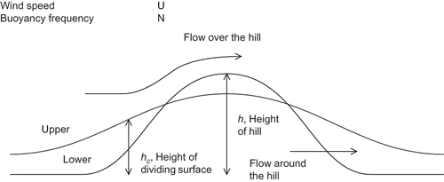
In this model of flow below the dividing surface, the terrain data are simplified to a single Gaussian-shaped hill of circular cross-section. Its height is taken to be the height of the highest hill and the horizontal length scale is the characteristic length scale of the terrain as calculated by FLOWSTAR. Then a dividing surface is defined that is also Gaussian in shape and based on the single idealized hill and with a horizontal length scale a factor of 10 greater than that of the idealized hill. Below the dividing surface, the flow is approximated by horizontal potential flow around the Gaussian-shaped hill used to represent the terrain except very close to the surface (lowest 10 m) when flow is assumed to be parallel to the actual surface on upstream slopes. Above the dividing surface, the stable flow field is assumed to follow the terrain; that is, streamlines remain at the same distance above the terrain with no convergence or divergence of streamlines with height. In order to smooth out any discontinuities in the flow field between Fr < 1 and Fr > 1, a weighted combination of the stable and FLOWSTAR flow fields is used when Fr < 1.

AERMOD

The AERMOD complex terrain model13 takes account of the effects of complex terrain on the dispersion of pollution in one stage using a quite different methodology from ADMS: it does not calculate the airflow over the complex terrain but directly calculates a weighted average of the concentration calculated for two cases, with the weighting dependent on the height of the dividing surface (streamline in AERMOD documentation; the terms will be used interchangeably). These two cases are (i) a horizontal plume (with concentration given by C _H) that impacts directly into the side of the hill (and reemerges from the other side of the hill) and (ii) a terrain following plume (with concentration given by C _T). Then the total concentration C is given by

(1)

The weighting factor f depends on the dividing streamline height (h _c) as discussed above. This is calculated from

(2)

where h is a receptor dependent terrain height scale. The weighting factor is given by

and ϕ by

(3)

There is always at least 50% plume impaction. When the plume is entirely above h _c, there is an equal weighting between the two cases (f = 0.5); when the plume is entirely below h _c (f = 1), only the horizontal plume contributes with impaction of all the plume onto the hillside.

AERMOD does not calculate any impacts of the terrain on mean flow or turbulence and hence on plume spread, nor does it allow for the impacts of hill wakes. In common with ADMS, the model does not take account of thermal winds induced in mountainous regions when there is little or no driving (regional) flow.

MODEL CALCULATIONS OVER COMPLEX TERRAIN

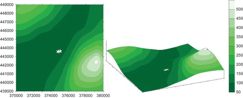
The stack parameters used for each site are shown in Table 1. Clifty Creek power station has a 208-m stack in a deep valley within a relatively flat landscape to the north some 150 m above the valley floor. The stack exit is some 60 m above the level of the valley top (Figure 2). Ribblesdale cement works (Figure 3) has two stacks of height 92 and 104 m and is situated in a valley with hilly terrain rising some 300 m above the valley floor.

Table 1. Stack parameters for the stacks in each of the cases

	Stack	Height (m)	Diameter (m)	Exit Velocity (m/sec)	Volume Flow Rate (m^3/sec)	Temperature (°C)	Emission Rate (g/sec)
Clifty Creek	Stack1	207.9	4.63	45*	—	172	2726*
	Stack2	207.9	4.63	46*	—	172	2756*
	Stack3	207.9	4.63	47*	—	172	2813*
Ribblesdale	Dry Kiln	92	2.3	—	115.8	160	168
	Wet Kiln	104	4.2	—	175	220	218.5
Notes: *This parameter varies hourly and this is the average value. In the case of Clifty Creek, plume rise was not accounted for and the exit velocities and temperatures were not used.

Figure 2. Terrain contour map and isometric projection for Clifty Creek. The stack is marked with a white star, the heights are in meters.

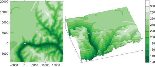
Figure 3. Terrain contour map and isometric projection for Ribblesdale. The stacks are marked with white stars, the heights are in meters.

Meteorology

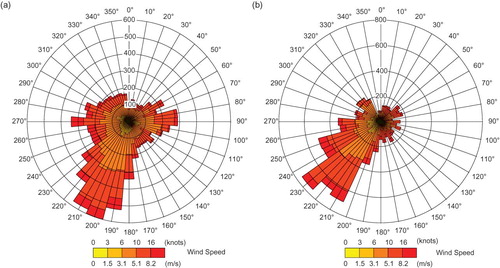
For the case of Clifty Creek, the meteorological data were measured on a 60m mast 3 km to the south of the power station. For the case of Ribblesdale, the data were obtained from a standard 10m meteorological mast at Waddington, which is distant (>100 km) from the works but has a similar climate. The meteorological parameters are summarized in Table 2 and wind roses are shown in Figure 4. Both sites exhibit prevailing winds in the sector between south and west and average wind speeds (measured at different heights) of about 5 m/sec in each case. Clifty Creek shows a higher percentage of light winds.

Table 2. Meteorological parameters used in the Clifty Creek and Ribblesdale calculation

	Clifty Creek				Ribblesdale
Data capture		100%			99.8%
Height (m)		10			10
Roughness length at met site (m)		0.2			0.5
	Statistics
	Mean	Minimum	Maximum	Mean	Minimum	Maximum
Temperature (°C)	12.0	−17.8	34.4	9.9	−4.8	26.5
Wind speed (m/sec)	5.0	0	21.1	4.7	0	15.5
Cloud cover (oktas)	5.0	0	8	5.5	0	8

Figure 4. Wind roses of wind data used for the (a) Clifty Creek and (b) Ribblesdale model calculations.

Clifty Creek

In the examples given for Clifty Creek, the effect of plume rise is not included in the calculations to maximize the impact of the complex terrain. Figure 5 presents contour plots of the annual mean concentrations for each of ADMS and AERMOD with and without the modeled impacts of complex terrain and also presents difference plots showing the difference in ADMS with and without complex terrain effects, the difference in AERMOD with and without terrain effects, the difference between ADMS and AERMOD with complex terrain, and the difference between ADMS and AERMOD without complex terrain. The concentrations are normalized by the emission rate. Note that in the figures the contours of terrain are shown only in the top two plots. A summary of the calculations is shown in Table 3, which shows the maximum values of the annual average and maximum hourly average concentration across the model domain.

Table 3. Maximum (and minimum) values for the average and maximum normalized concentrations for Clifty Creek

Model	Average Concentration (μsec/m^3)		Maximum Normalized Concentration (μsec/m^3)
ADMS hills	0.0464		10.40
ADMS no hills	0.0343		5.24
AERMOD hills	0.0251		5.01
AERMOD no hills	0.0265		5.21
	Minimum	Maximum	Minimum	Maximum
ADMS hills–ADMS no hills	−0.0017	0.0335	−1.25	6.21
AERMOD hills–AERMOD no hills	−0.0012	0.0052	−3.32	1.85
ADMS hills–AERMOD hills	0.0005	0.0355	−1.85	7.91
ADMS no hills–AERMOD no hills	−0.0021	0.0112	−2.41	2.52

Figure 5. Clifty Creek annual average concentrations normalized by the emission rate. Terrain elevation contours (black) are shown in the top two plots. The first four plots show concentrations calculated by the models, the second four plot differences in concentrations.

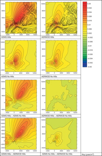
The model calculations for flat terrain, (No Hills)Figure 5 and Table 3, show that differences between the two models are relatively modest, with similar concentration patterns for the annual average and similar maximum values across the model domain of the maximum hourly concentration. Now comparing the cases taking account of complex terrain (Hills), ADMS predicts a significant impact of the terrain, with markedly higher maximum impacts for both annual average (35% increase) and maxima (100% increase), which are located downwind of the stack in the prevailing wind direction. This impact in ADMS is due to the FLOWSTAR airflow model predicting convergence of the mean streamlines as the airflow from the prevailing southwesterly direction flows out of the valley, which in turn brings the plume closer to the surface increasing surface concentrations. Conversely, the impact of complex terrain as calculated by AERMOD is relatively small. For this case where much of the terrain is below the height of the stack, the calculated fraction of plume mass below the dividing surface (ϕ) is zero so that the weighting factor (f) is given by f = 0.5 and therefore the source strength of the horizontal and terrain following plumes are of equal magnitudes.

Ribblesdale

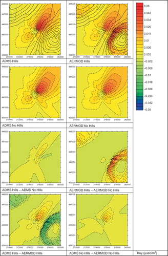
A similar set of contour plots and tables is presented for Ribblesdale Cement works in Figure 6 and Table 4. It is seen again that the two models predict relatively similar patterns of concentrations and similar peak values when the impact of complex terrain is not included in the calculations. When complex terrain is considered, ADMS shows a relatively small impact, with increases in maximum annual average and peak concentrations compared with the flat terrain values of less than 15%. In this case AERMOD (see southeast section of the difference plots for complex terrain) predicts very high concentrations on the side of the hills, with increases in maximum annual average of over 60% (even though this is not in the direction of the prevailing wind) and increases in peak hourly average concentrations of over 1800%. For this case, in some weather conditions (stably stratified, light winds), the plume height is below that of the hills to the southeast of the stack and the weighting factor (f) is close to 1; therefore AERMOD is predicting plume impaction into the hillside. For these same conditions, the ADMS airflow model predicts that the plumes are generally advected over the hill tops or around the hills and that plume impaction is not prevalent and is not markedly increasing concentrations.

Table 4. Maximum (and minimum) values for the average and maximum normalized concentrations for the Ribblesdale case

Model	Average Concentration (μsec/m^3)		Maximum Normalized Concentration (μsec/m^3)
ADMS hills	0.0470		1.01
ADMS no hills	0.0417		0.90
AERMOD hills	0.0518		10.36
AERMOD no hills	0.0316		0.54
	Minimum	Maximum	Minimum	Maximum
ADMS hills–ADMS no hills	−0.0027	0.0063	−0.11	0.53
AERMOD hills–AERMOD no hills	−0.0017	0.0416	−0.03	9.94
ADMS hills–AERMOD hills	−0.0421	0.0164	−9.90	0.60
ADMS no hills–AERMOD no hills	−0.0008	0.0104	−0.21	0.51

Figure 6. Ribblesdale annual average concentrations normalized by the emission rate. Terrain elevation contours (black) are shown in the top two plots. The first four plots show concentrations calculated by the models, the second four plot differences in concentrations.

CONCLUSIONS

Some results of the ADMS–AERMOD hybrid model have been used to compare the treatment of complex terrain in the two models without the complicating effects of the other differences between the two models such as the meteorological preporcessors.

In the first case presented of Clifty Creek, in which the source stack is positioned in a deep valley with stack top rising above the level of the surrounding terrain, ADMS suggests that the terrain has a significant effect and it predicts markedly different concentrations from the case of the same source over flat terrain. In this case AERMOD predicts that the impact of complex terrain is minimal.

In the second case, Ribblesdale, the differences between the two models is so large as to fundamentally change the scale of the impact on local air quality of the industrial site. These differences occur as the stack tops are below the height of the surrounding terrain when AERMOD predicts that, even in moderate levels of stable stratification (Fr > 1), plume impaction onto the hillside is an important process leading to high surface levels of concentration on the side of hills.

Given these differences, the question then arises as to which of the two models is the more accurate in the two different cases. Available field data and laboratory studies provide some insight. With regard to Clifty Creek, the field studies of airflow by Wiggs et al.14 and Mason15 show that as the air flows across the valley, there is slow down with streamline divergence and then speedup and hence streamline convergence towards the downwind edge of the valley. For a source located above the valley, this would suggest increased surface concentrations relative to the flat terrain case over the plateau downwind of the source, as predicted by ADMS. Note that comparisons of concentrations measured at six locations near Clifty Creek power station have been made for both ADMS16 and AERMOD17; however, although both models appear to perform reasonably, the comparisons provide relatively little insight into how well the two models are taking account of the impacts of the complex terrain because other factors such as differences in input meteorology arising from the two meteorological preprocessors may cause the model differences between the data and model predictions. With regard to Ribblesdale, studies in a stratified flume⁹ and at Cinder Cone Butte18 show that in stable conditions, there may be plume impaction onto the hillside. Both AERMOD and ADMS predict this to occur; however, AERMOD predicts markedly higher concentrations because there is no flow around the hill and hence the whole plume is assumed to impact onto the hillside, whereas the ADMS flow model predicts some horizontal deviation of the streamlines in these cases and hence the increase in concentrations at impaction is more modest.

From this we may conclude that where there is plume impaction, AERMOD has a tendency to overestimate concentrations and, therefore, may act as a screening model in this case, whereas ADMS may predict more realistic concentrations, but these concentrations may be overpredictions or underpredictions. Conversely, in the case of a source above a deep valley carved out of a plain (as at Clifty Creek), AERMOD suggests that the effects of the terrain are very small because the stack exit is higher than most nearby terrain; this may result in an underestimate of concentrations in such situations. ADMS includes the effect of valleys on airflow but there are insufficient field data with which to ascertain the model accuracy in this case.

REFERENCES

- Carruthers , D.J. , Holroyd , R.J. , Hunt , J.C.R. , Weng , W.S. , Robins , A.G. , Apsley , D.D. , Thomson , D.J. and Smith , F.B. 1994 . UK-ADMS: A New Approach to Modelling Dispersion in the Earth's Atmospheric Boundary Layer . J. Wind Eng. Ind. Aerodyn. , 52 : 139 – 153 .
- ADMS 4 Technical Specification. Cambridge Environmental Research Consultants Web site http://www.cerc.co.uk/environmental-software/model-documentation.html#technical (http://www.cerc.co.uk/environmental-software/model-documentation.html#technical)
- Cimorelli , A.J. , Perry , S.G. , Venkatram , A. , Weil , J.C. , Paine , R.J. , Wilson , R.B. , Lee , R.F. , Peters , W. , Brode , R. and Paumier , J.O. September 2004 . AERMOD: Description of Model Formulation; EPA-454/R-03-004 , September , U.S. Environmental Protection Agency , NC : Research Park Triangle .
- Model Evaluation Databases. U.S. Environmental Protection Agency Web site http://www.epa.gov/scram001/dispersion_prefrec.htm (http://www.epa.gov/scram001/dispersion_prefrec.htm)
- Carruthers , D.J. , McHugh , C.A. , Vanvyve , E. and Solazzo , E. 2009 . “ Comparison of ADMS and AERMOD Meteorological Preprocessor and Dispersion Algorithms ” . In Proceedings of Air & Waste Management Association, Air Quality Models: Next Generation of Models, Rayleigh NC, October 28-30 , Pittsburgh , PA : Air & Waste Management Association . 2009 [CD-ROM]. Paper 2010
- The Met Input Module. The UK Met Office; Cambridge Environmental Research Consultants Web site http://www.cerc.co.uk/environmental-software/assets/data/doc_techspec/CERC_ADMS4_P05_01.pdf (http://www.cerc.co.uk/environmental-software/assets/data/doc_techspec/CERC_ADMS4_P05_01.pdf)
- Clifty Creek Power Plant. Cambridge Environmental Research Consultants Web site http://www.cerc.co.uk/environmental-software/assets/data/doc_validation/CERC_ADMS4_Study_Validation_Clifty_Creek%204.1_vs_4.2.pdf (http://www.cerc.co.uk/environmental-software/assets/data/doc_validation/CERC_ADMS4_Study_Validation_Clifty_Creek%204.1_vs_4.2.pdf)
- Carruthers , D.J. and Hunt , J.C.R. June 1990 . “ Fluid Mechanics of Airflow over Hills: Turbulence, Fluxes, and Waves in the Boundary Layer. In Blumen, W ” . In Atmospheric Process over Complex Terrain , June , 83 – 107 . American Meteorological Society : Botson, MA .
- Hunt , J.C.R. and Snyder , W.H. 1980 . Experiments on Stably and Neutrally Stratified Flow over a Model Three-Dimensional Hill . J. Fluid Mech. , 96 : 671 – 704 .
- Smith , R.B. 1979 . The Influence of Mountains on the Atmosphere . Adv. Geophys. , 21 : 87 – 230 .
- Complex Terrain Module. Cambridge Environmental Research Consultants Web site http://www.cerc.co.uk/environmental-software/assets/data/doc_techspec/CERC_ADMS4_P14_01.pdf (http://www.cerc.co.uk/environmental-software/assets/data/doc_techspec/CERC_ADMS4_P14_01.pdf)
- FLOWSTAR User Guide. Cambridge Environmental Research Consultants Web site http://www.cerc.co.uk/environmental-software/assets/data/doc_userguides/CERC_FLOWSTAR7.1.4_User_Guide.pdf (http://www.cerc.co.uk/environmental-software/assets/data/doc_userguides/CERC_FLOWSTAR7.1.4_User_Guide.pdf)
- Venkatram , A. , Broke , R. , Cimorelli , A. , Lee , R. , Paine , R. , Perry , S. , Peters , W. , Weil , J. and Wilson , R. 2001 . A Complex Terrain Dispersion Model for Regulatory Applications . Atmos. Environ. , 35 : 4211 – 4221 .
- Wiggs , G.F.S. , Bullard , J.E. , Garvey , B. and Castro , I. 2002 . Interactions between Airflow and Valley Topography with Implications for Aeolian Sediment Transport . Phys. Geogr. , 23 : 366 – 380 .
- Mason , P.J. 1987 . Diurnal Variations in Flow over a Succession of Ridges and Valleys . Q. J. R. Meteorol. Soc. , 113 : 1117 – 1140 .
- Clifty Creek Power Plant. Cambridge Environmental Research Consultants Web site http://www.cerc.co.uk/environmental-software/assets/data/doc_validation/CERC_ADMS4_Study_Validation_ Clifty_Creek%204.1_vs_4.2.pdf (http://www.cerc.co.uk/environmental-software/assets/data/doc_validation/CERC_ADMS4_Study_Validation_ Clifty_Creek%204.1_vs_4.2.pdf)
- Perry , S.G. , Cimorelli , A.J. , Paine , R.J. , Brode , R.W. , Weil , J.C. , Venkatram , A. , Wilson , R.B. , Lee , R.F. and Peters , W.D. AERMOD . 2005 . A Dispersion Model for Industrial Source Applications. Part II: Model Performance against 17 Field Study Databases . J. Appl. Meteorol. , 44 : 694 – 708 .
- U.S. Environmental Protection Agency . 1984 . Description of a Computer Database for Small Hill Impaction Study No. 1, Cinder Cone Butte, Idaho; U.S. EPA 600/3-84-038 , Research Park Triangle , NC : Environmental Sciences Research Laboratory .