Black carbon particulate matter emission factors for buoyancy-driven associated gas flares

Abstract

Flaring is a technique used extensively in the oil and gas industry to burn unwanted flammable gases. Oxidation of the gas can preclude emissions of methane (a potent greenhouse gas); however, flaring creates other pollutant emissions such as particulate matter (PM) in the form of soot or black carbon (BC). Currently available PM emission factors for flares were reviewed and found to be questionably accurate, or based on measurements not directly relevant to open-atmosphere flares. In addition, most previous studies of soot emissions from turbulent diffusion flames considered alkene or alkyne based gaseous fuels, and few considered mixed fuels in detail and/or lower sooting propensity fuels such as methane, which is the predominant constituent of gas flared in the upstream oil and gas industry. Quantitative emission measurements were performed on laboratory-scale flares for a range of burner diameters, exit velocities, and fuel compositions. Drawing from established standards, a sampling protocol was developed that employed both gravimetric analysis of filter samples and real-time measurements of soot volume fraction using a laser-induced incandescence (LII) system. For the full range of conditions tested (burner inner diameter [ID] of 12.7–76.2 mm, exit velocity 0.1–2.2 m/sec, 4- and 6-component methane-based fuel mixtures representative of associated gas in the upstream oil industry), measured soot emission factors were less than 0.84 kg soot/10³ m³ fuel. A simple empirical relationship is presented to estimate the PM emission factor as a function of the fuel heating value for a range of conditions, which, although still limited, is an improvement over currently available emission factors.

Implications

Despite the very significant volumes of gas flared globally and the requirement to report associated emissions in many jurisdictions of the world, a review of the very few existing particulate matter emission factors has revealed serious shortcomings sufficient to suggest that estimates of soot production from flares based on current emission factors should be interpreted with caution. New BC emissions data are presented for laboratory-scale flares in what are believed to be the first such experiments to consider fuel mixtures relevant to associated gas compositions. The empirical model developed from these data is an important step toward being able to better predict and manage BC emissions from flaring.

Introduction

Flaring is the common practice of burning off unwanted, flammable gases via combustion in an open-atmosphere, non-premixed flame. This gas may be deemed uneconomic to process (i.e., if it is far from a gas pipeline or if it is “sour” and contains trace amounts of toxic H₂S) or it may occur due to leakages, purges, or an emergency release of gas in a facility. Estimates derived from satellite imagery suggest more than 139 billion cubic meters of gas were flared globally in 2008 (Elvidge et al., 2009) Although the composition of flared gas can vary significantly, within the upstream oil and gas (UOG) industry, generally, the major constituent is methane. Since methane has a 25 times higher global warming potential (GWP) (on a 100 year time-scale) than CO₂ on a mass basis (Solomon et al., 2007), flaring can preclude significant greenhouse gas emissions that would occur if the gas were simply vented into the atmosphere. However, flaring can produce soot and other pollutant species that have negative effects on air quality and the environment (Johnson and Kostiuk, 2000; Johnson et al., 2001; Pohl et al., 1986; Strosher, 2000). Soot is implicated as a significant health hazard primarily because of its small size (Pope et al., 2002), and it has been linked to serious, adverse cardiovascular, respiratory, reproductive, and developmental effects in humans (U.S. Environmental Protection Agency [EPA], 2010). Soot has also been recognized as an important source of anthropogenic radiative forcing of the planet's surface (Hansen et al., 2000; Ramanathan and Carmichael, 2008; Solomon et al., 2007) The key objectives of this paper are to review and critically assess current understanding of soot emissions from flares typical of the upstream oil and gas industry, and to present results of experiments aimed at developing a better methodology for accurately predicting these critical emissions.

Estimates of emissions from flaring are complicated by the large diversity of flare designs, applications, and operating conditions encountered. Industrial flares may be broadly classed as emergency flares, process flares, or production flares (Brzustowski, 1976; Johnson and Coderre, 2011). Emergency flaring is by definition intermittent and typically involves large, very short duration, unplanned releases of flammable gas that is combusted for safety reasons. Flare stack exit velocities during emergency flaring can approach sonic. Process flaring may involve large or small releases of gas over durations ranging from hours to days, as is encountered in the upstream oil and gas industry during well testing to evaluate the size of a reservoir, or at downstream facilities during blow-down or evacuation of tanks and equipment. Production flaring typically involves smaller, more consistent gas volumes and much longer durations that may extend indefinitely during oil production, in situations where associated gas (a.k.a. solution gas) is not being conserved. The design of a flare can also vary significantly, ranging from simple pipe flares (essentially an open-ended vertical pipe) that are common in the UOG industry, to flares with engineered flare tips that can include multiple fuel nozzles and multipoint air and/or steam injection for smoke suppression (Brzustowski, 1976). In terms of emissions, key factors that can affect flare performance include the exit velocity of gas from the flare, the flare gas composition, ambient wind conditions, flare stack diameter, and flare tip design (Johnson and Kostiuk, 2000, 2002a).

Previous Emissions Measurements from Flares

Despite the ubiquity of flares in the world, there have been relatively few successful studies investigating their emissions (Johnson and Kostiuk, 2000, 2002a; Johnson et al., 2001; Kostiuk et al., 2000, 2004; Pohl et al., 1986; Pohl and Soelberg, 1985; Siegel, 1980; Strosher, 2000), and most have focused on quantifying gas-phase carbon conversion efficiencies. Progress has been hampered by the inherent difficulties in accurately sampling emissions from an unconfined, turbulent, inhomogeneous, elevated plume of a flare. General understanding is further complicated by the incredibly wide range of operating conditions (i.e., exit velocities, crosswind conditions, fuel compositions) encountered in different applications. For pilot-scale flares in the absence of cross-flow, both Pohl et al. (1986) and Siegel (1980) traversed a sample probe above the flare and found gas-phase carbon conversion efficiencies in excess of 98%, except at low heating values near the limits of flame stability (Pohl et al., 1986). Although Siegel attempted to consider effects of moderate crosswinds using a blower system, because of problems measuring velocities in the unsteady plume, he was only able to report “local” conversion efficiencies based on ratios of gas-phase species concentrations at the location of the sample probe. Nevertheless, for the high hydrogen flare gas mixture (54.5% H₂, 42.8% C₁–C₆ hydrocarbons) considered by Siegel, he found local efficiencies typically above 95% in low-moderate crosswinds up to ∼5 m/sec. These results stand in contrast to single-point field measurements by Strosher (Strosher, 2000,1996) taken downstream of two “solution gas” flares (i.e., low-exit-velocity flares at upstream oil production facilities burning gas released from solution when produced oil is brought to the surface). Strosher found local efficiencies (calculated to include carbon emissions from the flare) ranging from 62% to 84% downstream of the flame tip and suggested that these lower efficiencies might be linked to carry-over of liquids into the flare gas stream. However, it has been shown for both pilot-scale vertical flares (Pohl et al., 1986), and laboratory-scale flares in cross-flow (Poudenx, 2000; Howell, 2004), that the composition of the product plume is inhomogeneous, which presents a significant challenge in interpreting efficiency measurements derived from single-point samples of the plume. Pohl et al. (1986) showed that the fraction of unburned hydrocarbons could vary by more than a factor of two across the plume.

Apart from the few known pilot-scale studies cited above, most general understanding of the factors affecting flare emissions has been derived from wind tunnel testing of laboratory-scale flares under controlled conditions. Data from experiments in a closed-loop wind tunnel where the entire plume of products from the flare could be captured (Bourguignon et al., 1999; Johnson and Kostiuk, 2000; Johnson et al., 2001; Johnson and Kostiuk, 2002a) have shown that in the case of low-exit-velocity (∼0.5-5 m/sec) pipe flares burning hydrocarbon fuel mixtures with heating values equal to or greater than that of natural gas (∼37 MJ/m³), gas-phase efficiencies above 98–99% could be expected at low crosswind speeds. However, efficiencies reduced rapidly at high crosswind speeds, with a functional dependence that varied with , where is the crosswind velocity and is the exit velocity of the flare gas. Inefficiencies under these conditions were primarily in the form of unburned fuel driven by a coherent-structure-based fuel stripping mechanism (Johnson et al., 2001; Johnson and Kostiuk, 2002b). Experiments also revealed quite low efficiencies at flare gas heating values below ∼20 MJ/m³ (Johnson and Kostiuk, 2000, 2002a; Kostiuk et al., 2004), which was the impetus for regulatory changes to the minimum permissible flare gas heating value in the Province of Alberta, Canada (ERCB Directive 60, 2006). A crude parametric model was proposed for low-momentum, hydrocarbon pipe-flares in cross-flow based on these results (Johnson and Kostiuk, 2002a); however, because of the empiricism in the model, it is limited to the range of conditions considered in the experiments.

Previous measurements of soot emissions from flares

In one of the few works to consider soot emissions from flares, McDaniel (1983) collected soot samples on filters for gravimetric analysis using a single-point probe suspended above a 203.2-mm-diameter pilot-scale flare burning “crude propylene” (approximately 80% propylene, 20% propane) with exit velocities from 2.3 to 4.2 m/sec. The typical flare in McDaniel (1983) used steam for smoke suppression during experiments to measure combustion efficiency. However, for the conditions where soot was measured, the steam flow was disabled to purposefully produce a smoking flare. The soot measurements made in this work were reported in terms of exhaust gas soot concentration only, and since the dilution of the samples was not known, data were not directly relatable to fuel consumption as is standard with emission factors.

Pohl et al. (1986) investigated the effect of soot on combustion efficiency from pilot-scale flares burning propane with burner diameters ranging from 76.2 to 304.8 mm and exit velocities ranging from 0.03 to 30 m/sec. Soot was captured on a “filter at the end of a probe, and its concentration [was] determined by burning combustibles from the filter” (Pohl et al., 1986). Although soot concentrations or emission rate data were not directly reported, the authors concluded that soot emissions accounted for “less than 0.5 percent of the combustion inefficiencies for most of the conditions tested” (Pohl et al., 1986).

In the only other known study to specifically consider soot emissions from a flare, the Ph.D. thesis of Siegel (1980) attempted to indirectly quantify soot emissions as the residual carbon from a mass balance on measurable gas-phase carbon-containing species. The pilot flare in the tests of Siegel used a commercial flare tip with a diameter of 700 mm burning a refinery relief gas mixture with exit velocities from 0.1 to 2.5 m/sec. The refinery relief gas mixture had a high concentration of hydrogen (55% on average) and would be expected to produce less soot upon stable operation. Although Siegel was able to conclude that in the absence of crosswind, the gas-phases efficiencies were unchanged by the presence of visible soot emission, the uncertainties in closing the carbon mass balance were too high to reliably estimate soot emissions themselves. In one particular test, four single-point filter samples of soot were taken above the flare but measured concentrations varied by a factor of 3.5, and Siegel cautioned that it was impossible to specify an emission factor for soot in a flare and his results should be used as reference only (quoted in German as: “Es sei aber nochmals darauf hingewiesen, dass die Angabe eines Emissionsfaktors für Ruß bei Fackelflammen nicht möglich ist und dass die hier aufgeführten Werte als Orientierung und nicht als bindend gewertet werden sollten” (Siegel, 1980)).

Recently, a new technique for directly measuring mass flux of soot from visibly sooting flares under field conditions has been demonstrated (Johnson et al., 2010, 2011). Although this approach has promise as a potential monitoring technique for flare emissions, it is still under development. To date, the technique has only been applied to a single, large, visibly sooting flare for which emissions of 2.0 ± 0.66 g/sec were measured; approximately equivalent to “soot emissions of ∼500 buses constantly driving” (Johnson et al., 2011).

None of the studies cited above specifically considered the effects of crosswind on soot emissions. Increased wind speeds have been shown to reduce the overall combustion efficiency of flares (Johnson and Kostiuk, 2000, 2002a; Johnson et al., 2001; Kostiuk et al., 2004); however, limited available data suggest that the increased mixing of ambient air can slightly decrease the amount of soot produced (Kostiuk et al., 2004). This observation is consistent with the only other known study in this regard (Ellzey et al., 1990), which examined small-scale (1.04 to 2.16 mm diameter) propane diffusion flames under cross-flow and co-flow conditions. The current research focuses on the quiescent wind conditions only (i.e., zero cross-flow), which should represent the “worst-case” sooting scenario.

Current PM_2.5 Emission Factors

Given the state of knowledge and lack of available models to predict soot emissions from flares, it is worth briefly examining how emission estimates for pollutant inventories and regulatory decisions are currently derived. In most developed jurisdictions throughout the world, key pollutants such as particulate matter less than 2.5 μm in diameter (PM_2.5), which includes soot from flares, must be reported and are tracked in government emission inventories. Emissions are generally estimated using simple emission factors that specify a unit of pollutant emitted per unit of fuel consumed. Given the wide variation in flare emissions associated with large variations in meteorological conditions, fuel composition, fuel flow rates, flare size, and flare design, this approach to estimating emissions is at best overly simplified.

Existing PM_2.5 emission factors for flares are essentially limited to three sets of values published in the EPA WebFIRE database (EPA, 2009), as summarized in Table 1 and converted to common units for comparison. These include a factor from a confidential report based on landfill gas flares (EPA, 1991), a factor from AP-42 section 2.4 (1998) from landfill gas flares, and a factor from AP-42 section 13.5 (EPA,1995) from industrial flares. Emission factors in other jurisdictions (e.g., Canada) are typically based on these data due to the general lack of measurements available on PM_2.5 from flares. For the UOG industry in Canada, the Canadian Association of Petroleum Producers (CAPP) has produced a guide (CAPP, 2007) to help industry members report their emissions to the National Pollutant Release Inventory (NPRI) as required. The emission factor used to estimate production of soot from flares in Canada (also shown in Table 1) is derived from the emission factor attributed to the confidential report from the EPA entitled “Data from flaring landfill gas” (EPA, 1991). This emission factor is published in U.S. EPA's WebFIRE database as 0.85 kg soot per 10³ m³ of fuel (EPA, 2009). The CAPP guide instead gives a value of 2.5632 kg soot per 10³ m³ of fuel and notes that the EPA value has been “corrected” for a gas with a heating value of 45 MJ/m³. The CAPP guide does not specify how this apparent factor of 3 correction was derived, although it likely resulted from an assumed linear scaling of soot emission with heating value, since landfill gas could be expected to have a heating value on the order of 15 MJ/m³, and a heating value of 45 MJ/m³ should be typical of flare gas in the UOG industry.

Table 1. Comparison of current soot emission factors for flares

Standard	Original Emission Factor	EF (kg PM per10^3 m^3 of Fuel)	Fuel Gas
U.S. EPA FIRE 6.25 (U.S. Environmental Protection Agency, 2009)	53 lb PM per 10^6 ft^3 gas	0.85	Landfill gas ^a
	17 lb PM per 10^6 ft^3 gas	0.27	Methane
	0, 40, 177, 274 lb PM per 10^6 BTU	0, 1500, 6634, 10270 ^b	80% propylene 20% propane
CAPP guide (CAPP, 2007)	2.5632 kg PM per 10^3 m^3 fuel	2.5632	Associated gas
U.S. EPA AP-42 Vol. I, section 13.5 (U.S. Environmental Protection Agency, 1995)	0, 40, 177, 274 ^c μg PM per 10^−3 m^3 exhaust gas	0, 0.9, 4.2, 6.4 ^d	80% propylene 20% propane
Notes: ^aAlthough the source for this emission factor is not publicly available and the composition of landfill gas varies, a typical composition could be 56% methane, 37% CO2, 1% O2, and trace amounts of other gasses (Eklund et al., 1998).
^bBased on a fuel heating value of 87 MJ/m^3 (1 BTU = 1055.06 J).
^cThe four different values are based on the “smoking level” of the flare: non-smoking flares, 0 μg/L; lightly smoking flares, 40 μg/L; average smoking flares, 177 μg/L; and heavily smoking flares, 274 μg/L (U.S. Environmental Protection Agency, 1995).
^dThese emission factors were calculated by the present authors from the original reported exhaust gas emission factors, assuming no dilution and simple combustion chemistry.

As can be seen in Table 1, the emission factors vary by orders of magnitude. Of the three different factors for flares reported in EPA's WebFIRE (EPA, 2009), the first two were largely derived from measurements on enclosed flares (although full details of the measurements are not publicly available), whereas burning gas compositions (pure methane and landfill gas) would have limited relevance to UOG flares. The third factor, as reported, is up to 5 orders of magnitude higher than the other two values. However, quite significantly, a review of the source data for this factor reveals an apparent clerical error in the form of a swap of units from μg PM per 10⁻³ m³ exhaust gas to lb PM per 10⁶ British thermal unit (BTU), between the emission factor as reported in EPA AP-42 (EPA, 1995) and the value reported in EPA WebFIRE (U.S. Environmental Protection Agency, 2009); both are attributed to the same data source (McDaniel, 1983). This error was formally reported to U.S. EPA and has been corrected in the EPA's draft review document “Emissions Estimation Protocol for Petroleum Refineries (v.2.0).”

Irrespective of reporting errors in these data, none of these factors is based on measurements from actual associated gas flares typical of the UOG industry (the CAPP guide value is derived from the EPA value), and none gives any consideration to operating conditions of a flare including wind speed, exit velocity, detailed fuel composition, flare size, or flare tip design, even though these parameters can significantly affect soot production. These discrepancies and simplifications bring into question the validity and credibility of the emission factors used for the significant global volumes of flared gas. The lack of accurate guidelines for estimating and reporting of soot from flares in the UOG industry is the primary motivation for the current work.

The Flare as a Vertical Diffusion Flame

Flares are elevated turbulent jet-diffusion flames. Jet-diffusion flames subjected to cross-flowing winds may be broadly categorized into two groups based on the momentum flux ratio, , where ρ is density, u is velocity, and the subscript j and ∞ denote the jet and cross-flow fluid respectively (e.g., Johnson and Kostiuk, 2000; Huang and Wang, 1999; Gollahalli and Nanjundappa, 1995). At high momentum flux ratios, the strength of the jet dominates, and the effects of the crosswind are relatively unimportant (Huang and Wang, 1999). At low momentum flux ratios, the flame bends over significantly in the wind and, at very low momentum flux ratios, the flame can be drawn down below the jet exit plane and become “wake-stabilized” on the leeward side of the stack (e.g. Gollahalli and Nanjundappa, 1995; Johnson and Kostiuk, 2000; Johnson et al., 2001).

Flares in quiescent wind conditions (i.e., high R) may be further categorized depending on whether the flame behavior is dominated by buoyancy of the hot gases or momentum of the reactants. Several studies on turbulent diffusion flames make use of a flame or fuel derived Froude number, Fr, to define the flame regime as momentum or buoyancy driven (Becker and Liang, 1978; Delichatsios, 1993a; Peters and Göttgens, 1991). Delichatsios (1993a) has elaborated on this notion to define a regime map for vertical turbulent diffusion flames, in which different flame regimes are defined depending on whether the turbulence is generated by instabilities present in the cold flow, or by the large buoyancy forces present in the flame. The “type” of turbulence generated will depend on the magnitude of the buoyancy forces to the inertia forces in the flame. Delichatsios (1993a) has identified these regimes as well as other subregimes based on the mode of transition from laminar to turbulent, in a graphical form as is shown in Figure 1. The main regimes of interest in the current work are the “turbulent-buoyant transition-buoyant” and “turbulent-buoyant transition-shear” regimes. It should be noted that the transitions between regimes are expected to be smooth, so that the dashed lines in Figure 1 should not represent a sudden change. The vertical axis of Figure 1 is simply the source Reynolds number based on the fuel properties, and the horizontal axis of Figure 1 is the fuel gas Froude number (Fr _g) (termed the modified fire Froude number by Delichatsios (1993a)), defined as shown in eq 1(1).

Figure 1. Regime map of turbulent jet-diffusion flames as proposed by Delichatsios (1993a) shown with relevant currently available soot emission measurement conditions from the literature. Shaded areas represent the estimated limits of test/operating conditions, rather than actual test points. The shaded inclined rectangle represents the expected operating regime of buoyancy-driven flares typical of the upstream oil and gas industry, with diameters ranging from 76.2 to 254 mm as shown, and exit velocities of 0.1 m/sec (values in the lower left of the shaded region) to 6 m/sec (values in the upper right).

(1)

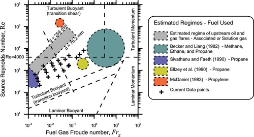
where u _e is the exit velocity (m/sec), f _s is the stoichiometric mixture fraction, g is the gravitational acceleration (m/sec²), d _e is the burner exit diameter (m), ρ _∞ is the ambient density (kg/m³), and ρ_e is the fuel density (kg/m³).

For continuous flares used to dispose of associated gas (a.k.a. solution gas) in the upstream oil and gas industry, an estimated range of expected conditions is identified by the inclined shaded rectangle in Figure 1. These conditions were calculated based on typical associated gas flares for Alberta, Canada (Johnson and Coderre, 2011; Johnson et al., 2001), where the bounding lower line represents a 76.2-mm burner and the upper line represents the 254-mm burner, and exit velocities span a range of 0.1 to 6 m/sec. According to the theory of Delichatsios (1993a), this range of flame conditions could all be classified as turbulent-buoyant, although they span both the transition-buoyant, and transition-shear subregimes. This information was used in determining flow conditions in an attempt to span both subregimes under the assumption that the subregime of the flame may impact the soot yield.

Previous Studies of Soot Emissions from Turbulent Diffusion Flames

Total soot emission from turbulent diffusion flames has been studied in the past (Becker and Liang, 1982; Delichatsios, 1993b; Sivathanu and Faeth, 1990). However, these works typically considered pure fuels comprised of heavier sooting alkene or alkyne hydrocarbons. Where alkanes have been studied, typically only propane has been considered. Becker and Liang (1982) studied soot emissions from the alkane family of fuels more thoroughly; however, to the authors' knowledge, their data are the only measurements of the total soot emission in the literature to include data from methane, ethane, and propane diffusion flames. Although they were not able to develop a theory for scaling soot emissions, they were able to demonstrate that the soot emission changed under varying flow conditions (i.e., burner size, exit velocity, fuel). The different flow conditions were identified by a Richardson ratio (Ri_L ), as defined in eq 2(2).

(2)

where L _f is the flame length (m). As can be seen, there is a heavy dependence of Ri_L on the flame length, and if flame length values vary slightly, large discrepancies in calculated Ri_L values can appear. Because the length of a turbulent flame is an ill-defined quantity, this flame length term is somewhat undesirable in terms of its sensitivity.

The work of Sivathanu and Faeth (1990) with propane also showed that soot emission varied with flow conditions, and proposed simple correlations of the measured soot emission with a smoke-point-normalized residence time, (where τ_R is the measured residence time and τ_sp is the measured smoke-point residence time). The smoke point of a fuel is an experimentally derived parameter that allows for comparisons of the sooting tendency between different fuels. Sivathanu and Faeth (1990) had defined residence time as the time interval between the interruption of the fuel flow (via a shutter that rapidly closed over the burner exit), and the disappearance of all flame luminosity.

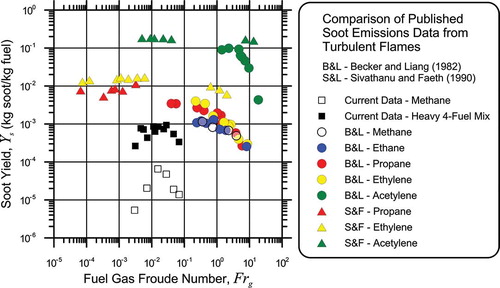
Both these works highlight the fact that soot emission changes with flow conditions and fuel, and a single emission factor applied to all conditions may be inappropriate. A comparison of these data, created by digitization of selected available raw data plots and shown in Figure 2, reveals further challenges. Specifically, the variation in soot yields spans several orders of magnitude, necessitating the use of a log scale to display the data. More curiously, while the data of Sivathanu and Faeth (1990) show the anticipated sensitivity of soot yield to fuel composition, the data of Becker and Liang (1982) suggest that in the range of Fr _g ≈ 5, the soot yields of methane, ethane, propane, and ethylene essentially overlap. The agreement between corresponding data sets of the two authors is not especially strong, especially for acetylene where the flow conditions appear to be similar (i.e., Fr _g ≈ 10) and soot yields vary by a factor of 4–8 or more. The present data for methane similarly do not align with data of Becker and Liang (1982), although the comparable experiments were at significantly different Froude numbers as indicated on the plot. In general, Figure 2 serves to show that where limited comparable data do exist for multiple flow conditions and fuels, there are still discrepancies. However, this may partially be attributed to that the fact that the Froude number in the work of Becker and Liang was calculated from the reported Richardson ratio, which could be expected to have a large variation based on the subjectivity of the flame length measurement.

Figure 2. Comparison of soot emission measurements from Becker and Liang (Becker and Liang, 1982), Sivathanu and Faeth (Sivathanu and Faeth, 1990), and current measurements using pure methane and the heavy 4-component fuel mix.

In another work of Delichatsios (1993b), simple soot emission measurements were made for several fuels, including propane, and a reasonable correlation for the scaling of soot yield with a calculated smoke-point heat release rate and stoichiometric ratio was presented, as shown in eq 3(3). The smoke-point heat release rate was calculated according to eq 4(4).

(3)

(4)

where is the mass flow rate at the smoke point and ΔH _c is the heat of combustion. Whereas the heat release is an easy parameter to monitor, the smoke-point heat release is difficult to calculate for multicomponent fuel mixtures. Compounding this problem is the lack of measurements of the smoke point for methane, since the flame becomes unstable before it starts to smoke in a standard smoke-point measurement test (Turns, 2000).

Glassman (1998) suggested that the flame temperature and length of time that soot particles reside at these elevated temperatures have a direct effect on the soot formation. Glassman postulated that what controls the soot volume fraction exiting the flame and causes soot emission is the distance between the isotherms that specify the incipient particle formation temperature and stoichiometric flame temperature (indicative of the strength of the temperature gradient). This distance establishes the growth time of the particles formed before flame oxidation of the soot occurs (Glassman, 1998). Although a universal theory for soot emission as a function of some temperature parameter is not given, it highlights the importance of the flame temperature on the soot formation.

Finally, Ouf et al. (2008) presented data on the effects of overventilating the flame on soot emissions. Specifically they were interested in changes in the size distributions of the primary particles and soot aggregates, morphology, and soot emission as a function of the global equivalence ratio. Ouf et al. found that the global equivalence ratio strongly influences the soot particle size, but does not play a predominant role in other soot morphological properties or emission rates (Ouf et al., 2008).

In short, a thorough review of the published literature on soot emissions of flares and vertical diffusion flames has revealed very few data that are directly relevant to the anticipated flow regimes and fuel compositions of flares typical of the upstream oil and gas industry. Furthermore, although a few different scaling parameters have been suggested, agreement among the limited comparable data currently available is generally poor. The controlled laboratory-scale experiments presented below provide new insight into this complex problem and represent important first steps toward developing practical models to predict soot emissions from flares.

Experimental Methods

Experiments were conducted in a laboratory-scale flare (LSF) facility, which consists of a vertical turbulent jet-diffusion burner and hooded sampling system as shown schematically in Figure 3. Fuel mixtures consisting of any or all of CH₄, C₂H₆, C₃H₈, C₄H₁₀, CO₂, and N₂ could be metered, mixed, delivered to the burner at fuel flow rates of up to 100 standard liters per minute (SLPM, evaluated at O°C and 101.325 KPa), and ejected from flare tips with exit diameters of 12.7, 25.4, 38.1, 50.8, or 76.2 mm. The entire combustion product plume and additional entrained room air were collected via a hood and drawn into a 152.4-mm-diameter insulated dilution tunnel (DT), which was vented to the atmosphere with a variable speed exhaust fan. Emissions were drawn from the DT and samples were collected on filters for later gravimetric analysis or routed directly to a laser-induced incandescence system (LII; Artium Technologies Inc., LII200; Sunnyvale, CA) for concentration measurement. Both data sets were used to calculate the total soot emission rates.

Figure 3. Schematic diagram of the laboratory-scale flare system. Modular burner detail shown with 25.4 mm I.D. exit and nozzle.

Fuel Mixture Compositions

Up to six separate components of the fuel mixtures (four hydrocarbons and two inerts) were chosen based on the analysis of data from associated gas samples at 2908 distinct upstream oil production sites in Alberta. These data were received as a private communication through the technical steering committee of the Petroleum Technology Alliance of Canada (PTAC), specifically to support this work (private communication between PTAC and M. R. Johnson, 2007). Analysis of these data has shown that methane is the major constituent of the gases being flared. To reduce the complexity of the experiment, surrogate mixtures were used based on the six most abundant components (i.e., mixtures of C1–C4, CO₂, and N₂). Higher hydrocarbons C5 through C7, He, and H₂ were not included in the test mixtures due to their very low concentrations. Thus, results of these experiments are primarily relevant to lighter hydrocarbon flare gas mixtures, which could be expected in upstream oil and gas flares with functioning liquid knockout systems (Kostiuk and Thomas, 2004). Hydrogen sulfide, H₂S, was also neglected primarily due to its extreme toxicity, but also because it was absent from most fuel mixtures (a.k.a. sweet gas). Although detailed speciation of hydrocarbon components was not available in the provided data, typical components in natural gas from both dry and wet reservoirs are alkane based (Smith et al., 1992). Furthermore, results from a limited sampling of six operating flares in Alberta have also confirmed that the principle hydrocarbons were all alkane based (Kostiuk and Thomas, 2004). Thus, in the present work the hydrocarbon fuel species C1 through C4 were assumed to be alkanes.

Average surrogate test mixtures of flare gas were created by scaling selected component concentrations by their concentrations in the full mixture. Lighter and heavier fuel mixtures were also created (Table 2) to investigate the effects of fuel composition on soot yield. To create the light mixture, the 90th percentile methane concentration was chosen as an upper bound, and the remaining fuel concentrations were determined based on their relative concentrations in the average fuel mixture (i.e., propane to ethane ratio constant, etc.). The heavy mixture was created in the same manner except that the 10th percentile methane concentration was chosen as a lower bound. The same process was repeated neglecting the diluents of CO₂ and N₂ to create 4-component fuel mixtures. The concentrations of all surrogate gas mixtures used in this study are summarized in Table 2.

Table 2. Average, light, and heavy 4- and 6-component fuel mixtures

		Average Mixture (%)		Light Mixture (%)		Heavy Mixture (%)
Species	Gas Purity (%)	6-Mix	4-Mix	6-Mix	4-Mix	6-Mix	4-Mix
Methane	99.0	85.24	88.01	91.14	91.14	74.54	74.54
Ethane	99.0	7.06	7.28	4.23	5.38	12.17	15.47
Propane	99.0	3.11	3.21	1.87	2.38	5.37	6.83
n-Butane	99.0	1.44	1.5	0.87	1.1	2.49	3.16
CO2	99.99	1.91	0	1.14	0	3.28	0
N2	99.999	1.24	0	0.75	0	2.15	0

Enclosure and Emission Collection System

The LSF enclosure was initially developed in the work of Canteenwalla (2007), and was designed based on the work of Sivathanu and Faeth (1990). The LSF burner is centered inside the 1.5 × 1.5 × 2.6 m tall sheet metal protective enclosure that sits 50 mm above the floor to allow easy air entrainment. A 1-m-diameter, 2-m-high mesh (690 wires/m, 0.23 mm wire diameter), open-ended cylindrical screen surrounds the flame to prevent buffeting of the flame from room currents. The front of the enclosure has two doors, one made of steel sheet metal, and the other of Plexiglas to provide visual access to the LSF. The top of the enclosure contracts and directs the entire exhaust plume and entrained dilution air into a 152.4 mm ID insulated, galvanized steel pipe. The 152.4-mm pipe acts as a dilution tunnel in which the combustion products and entrained room air are drawn by the exhaust fan and mixed prior to being sampled, as shown in Figure 3. The entrained room air was not separately filtered; however, measurements performed drawing samples from the system without the flame ignited showed that whatever particles were contained in the room air fell below detectable limits. The flow of diluted exhaust was assisted by an industrial centrifugal fan capable of drawing 13,000 LPM through the DT and controlled using a variable speed motor and controller. Calculations have shown (Canteenwalla, 2007) that once the system is warmed up to stable operating conditions, deposition of soot on the DT walls or sample line walls is negligible.

To establish a consistent, reliable test protocol, several pertinent measurement protocols for soot sampling from stationary sources were evaluated including the EPA Engine Testing Procedures (EPA, 2000), the U.S. EPA Emissions Measurement Center (EMC) Method 5—Particulate Matter from Stationary Sources (UNECE, 2008), and the UNECE Vehicle Regulation No. 49 (EPA, 1994). Although no specific guidelines existed for sampling from laboratory-scale flares, the consulted protocols were useful because they suggested general equipment and arrangements for the size of the DT, the DT flow rate measurement method, the sample probe type, the distance from the flow measurement and sample probe to the nearest disturbance, minimum DT flow rates, and conditions from the sample probe to the sampling device.

As shown in Table 3, the current system met or exceeded requirements from these three protocols, except where requirements of the different standards were contradictory, concerning dilution tunnel size and layout, dilution tunnel flow rate measurement, and sampling probe type and location. Ensuring that the exhaust gases were fully mixed within the DT was also critical. The fully mixed requirement was satisfied by ensuring that the Reynolds number in the DT was higher than 4000, and that the sample was sufficiently far downstream of any disturbances to ensure the exhaust gases were completely mixed. Good mixing was experimentally verified by traversing the DT with a probe to measure the soot volume fraction profile for both minimum and maximum expected DT flow rates.

Table 3. Comparison of sampling protocols

	Current Setup	EPA ETP (EPA, 2000)	UNECE Reg. 49 (EPA, 1994)	EPA EMC (UNECE, 2008)
Intended application	Laboratory-scale flares	PM from engines	PM from heavy vehicles	PM from stationary sources
DT diameter	6”	Not specified	>8”	4–12”
Flow measurement	Pitot rake, 17 measurements	Critical flow venturi, PDP, subsonic venturi, ultrasonic flowmeter	Critical flow venturi, PDP	Standard Pitot tube
Sample inlet	Pitot tube, 1/4”, upstream facing	Upstream facing probe	Upstream facing probe	Elbow or button hook (1/8–½”)
Disturbance to flow measurement	21.2 diameters	>10 diameters	Not specified	>16 diameters
Disturbance to sample inlet	24.47 diameters	Not specified	>10 diameters	>8 diameters
DT flow rates	Min Re of 10,000	Min Re of 4000	Min Re of 4000	Not specified
Temperature upstream of filter	<52 °C (maintained within ±5 °C)	47 ± 5 °C	<52 °C (maintained within ±3 °C)	120 ± 14° C
Isokinetic conditions?	No	Approximate	Yes	Within 10%
Sample device distance from sample port	0.5 m, insulated	As close as possible, insulated	<1.0 m	Immediate

When comparing sampling conditions among the cited sampling protocols, it became evident that all protocols controlled the temperature upstream of the sampling device (typically a filter assembly) as opposed to controlling the dilution ratio (DR = Q _{Diultion Air}/Q _Products). A protocol was therefore developed based on monitoring and controlling the temperature upstream of the measurement device as opposed to specifying a fixed dilution ratio or dilution ratio range, as further discussed below under “Sampling Protocol.” This led to the use of a secondary dilution device that added filtered room temperature air upstream of the soot measurement device (as shown in Figure 3) to cool the exhaust gases when specifically required. The three referenced protocols all suggested a different upstream temperature, so the median value of 52 ± 5 °C was chosen for the current protocol.

Soot Sampling System

Two different measurement devices were used to measure the soot volume fraction in the sample gas stream as highlighted in Figure 3: a gravimetric sampling system and a laser-induced incandescence (LII) instrument. The gravimetric system used 47-mm PTFE (Polytetrafluoroethylene) membrane filters (Fluoropore FGLP04700; Millipore: Billerica, MA). Filter handling procedures (i.e., clean room temperature and humidity settings, filter charge neutralization, filter weighing procedures) were completed according to EPA TP 714C (1994) to determine the mass of soot collected, and when combined with the volume of sample gas drawn through the filter face and a soot density (Canteenwalla, 2007), the soot volume fraction (f_v ) could be found (McEwen, 2010). LII is a laser-based technique used to determine soot volume fraction in real time. The reader is referred to Snelling et al. (2005) for a detailed description of the theory behind its operation. The LII instrument used in the current work provided real-time measurements of f_v at a sample rate of 20 Hz. With either measurement technique, the resultant f_v values were combined with other measured parameters defined in eq 5(5) to produce the soot yield, Y _s, defined as the mass of soot produced per mass of fuel burned (McEwen, 2010).

(5)

where ρ_soot is the soot density (kg/m³), f_{v ,sample} is the soot volume fraction at the sample location measured by either technique, Q _DT is the dilution tunnel flow rate (m³/sec), T _sample is the gas temperature at the sample location (K), T _DT is the gas temperature in the dilution tunnel (K), and is the fuel mass flow rate (kg/sec). The temperature ratio is necessary to correct the sample location soot volume fraction to the DT condition soot volume fraction. It is noted that eq 5(5) implicitly assumes that all soot was generated from the flare (as verified by a lack of detectible soot particles when tests were run without igniting the flame).

Sampling Protocol

A standard protocol was developed to ensure repeatable results. Of specific importance were the warm-up time, DT conditions, and sampling duration. The warm-up time was determined by monitoring several different temperature measurements on start-up, including the gas temperatures at the burner exit, inside the enclosure, in the DT, and upstream of the filter or heated sampling line. Once these temperatures reached stable values (generally around ∼30 min), testing would commence.

The fan speed was then fine-tuned to regulate the sample temperature directly upstream of the filter by increasing or decreasing the amount of primary dilution air, in line with the protocol discussed above. If the primary dilution air alone was insufficient to cool the exhaust gases to the desired temperature, the secondary dilution device was activated to add a controlled amount of filtered building air to the sample. Although control of the exhaust gas temperature was not deemed necessary for LII operation, it was decided that conditions for measurements should be identical between gravimetric and LII tests.

Isokinetic sampling was not required in the present experiments due to the small size of the soot particles, as verified in three ways. Firstly, calculations using scanning mobility particle sizing (SMPS) data extracted from directly above the flame showed that Stokes numbers of the soot aggregates were less than 0.01 for all conditions found in the experiments. At these low Stokes numbers, the particles track the flow very efficiently, and fully representative samples would be collected even if the mismatch between the main flow and sample probe velocities was an order of magnitude or greater (Hinds, 1999). Secondly, during the design of the experiment, the sampling system was sized so that the sampling duct to sample probe velocity ratio would fall as closely as possible to unity, and near isokinetic sampling would be achieved over the majority of operating conditions (never falling outside the range of 40–110% of the isokinetic sampling velocity). Thirdly, specific verification experiments were performed in which the direction of the sample probe within the sampling duct was rotated 180° to face away from the flow. Even under this extreme anisokinetic condition, samples matched those collected with the probe correctly positioned, which experimentally verified the prediction from the Stokes number calculations.

Although the reviewed sampling protocols all specified sample temperatures rather than dilution ratios, it is noted that some authors (Canteenwalla, 2007; Ouf et al., 2008; EPA, 2005) have cited dilution ratio as a parameter that can affect both the particle size, as well as the measured soot volume fraction. To ensure that the current sampling protocol was appropriate, and specifically to ensure that the dilution ratio in the sampling tunnel did not affect the measurements so long as the constant sample temperature condition was met, several tests were carried out using the 25.4-mm burner at 0.5 m/sec burning the average 6-component fuel mixture. The fan speed was varied from 20% to 100%, whereas the temperature upstream of the sample location was held to <52 °C using the secondary dilution device when necessary. The results of these tests for both gravimetric and LII results showed negligible differences in the measured soot mass emission rate at the different fan speeds used, establishing the robustness of the current protocol. This is consistent with the conclusions of Ouf et al. (2008), who in their study of overventilated diffusions flames showed that the global equivalence ratio does not play a predominant role in the global mass production of soot particles emissions. Furthermore, during these tests the sample flow rate changed based on the amount of secondary dilution added, and the consistency of results was a further experimental verification that isokinetic sampling was not necessary in the present case, since the change in the strength of the sink (the sample probe) in the DT did not affect the measured soot yield.

The sampling duration for gravimetric tests was based on the minimum amount of sample required to ensure reasonable uncertainties. It was determined that a minimum of 50 μg of soot should be obtained for each filter test to ensure reasonable uncertainties (less than ∼15%). By basing the test time on the amount of soot required, this meant that the test time could vary between 5 min for heavy-sooting conditions to 1 hr for low-sooting conditions. Test duration for the LII tests was determined via a convergence criterion applied to the time resolved data as it was recorded. The confidence interval (95% confidence level) of the test was calculated and a test was considered complete when this value was less than 0.5% of the mean, meaning that the calculated uncertainty and averaged measurement became stable.

During LII operation, anomalous soot volume fraction data points (1–2 orders of magnitude above the average) were occasionally observed. These erroneous data points resulted in large confidence intervals and were most likely due to large dust particles in the room air or possibly large soot particles deposited on the DT or sampling line walls being re-entrained into the flow. Chauvenet's criterion was used to filter these erroneous points from the soot volume fraction data output from the LII instrument. Chauvenet's criterion will discard a data point if the probability of obtaining the particular deviation from the mean is less than 1/(2n), where n is the total number of sample points.

Uncertainty Analysis

A detailed uncertainty analysis was conducted based on the ANSI/ASME Measurement Uncertainty Standard (ANSI/ASME, 1985), which considers separate contributions of the systematic error (alternatively called bias error or instrument accuracy), denoted by B, and the precision error (or random error), denoted by P, to the total uncertainty (displayed in results figures as error bars). The standard assumes that the systematic uncertainties encountered are normally distributed. Each component error is estimated separately and then combined into a final uncertainty, U, in quadrature. The precision error is calculated by multiplying the standard error of the sample average by the appropriate 95% confidence interval t value from the Student's t distribution table as , where σ is the sample standard deviation, N is the sample size, and the subscript v is the degrees of freedom (N − 1). The systematic and precision errors are assumed independent and combined in quadrature by the root sum of the squares method to produce an approximate total uncertainty, . The precision error is only calculated at the final stage of uncertainty analysis, as it is assumed that the scatter in contributing components of the final uncertainty will be propagated to the scatter of the final calculated value. For example, if is an average of N measurements of g, and g is a function of x and y, each of which have an associated precision error, the final precision of is calculated as the scatter on g, where the precision error will reflect both precision errors within tests, and variation among tests.

Results and Discussion

Soot yield values were determined using both measurement techniques for a large data set that included multiple burner diameters, a range of fuel exit velocities, and different 4- and 6-component fuel mixtures. Results obtained using the two different approaches are plotted in Figure 4, which shows good linear correlation (r ² = 0.92) within the calculated uncertainty limits displayed with error bars on the individual measurement points. The LII measured soot yield values are consistently lower than gravimetric measured soot yield values, which is expected since the LII technique heats the soot particles to temperatures approaching 4000 K, evaporating or sublimating all volatile components that may be condensed on the soot particles. Soot measured in this sense, i.e., by an optical absorption or emission based method, is commonly referred to as black carbon (BC), whereas the gravimetric values represent the total carbon. The difference between the two measurements is attributable to the organic carbon (OC) fraction of the soot particles. The slope implies a mean black carbon to total carbon fraction of 0.80 in the emitted soot, although a measurement based on the National Institute for Occupational Safety and Health (NIOSH) 5040 standard is likely to be better suited for accurately determining the relative carbon fractions in soot aggregates. Nevertheless, the agreement between these two techniques gives an important confidence in the measured results. Since the black carbon emissions are of particular interest in this work, only the LII recorded measurements will be discussed henceforth.

Figure 4. Comparison of LII and gravimetric measured soot yield.

Scaling Soot Emissions

Several parameters cited in the literature were used in an attempt to scale soot emissions with flow conditions, including the fire Froude number, Fr _f (Delichatsios, 1993a), the Richardson ratio, Ri_L (Becker and Liang, 1982), the residence time, τ_R (Sivathanu and Faeth, 1990), and a smoke-point-normalized soot generation efficiency, SGE_sp (Canteenwalla, 2007). Of these, the fire Froude number suggested by Delichatsios (1993a) proved the most effective. The Fr _f is similar to the fuel gas Froude number defined in eq 1(1), but includes an extra temperature ratio to account for flow acceleration due to buoyant forces produced in the flame, as defined in eq 6(6).

(6)

where ΔT _f is the characteristic temperature rise from combustion, typically calculated as the adiabatic flame temperature minus the ambient temperature (K), and T _∞ is the ambient temperature (K). Soot yield is plotted as a function of the fire Froude number in Figure 5 for the average-mix 6-component fuel.

Figure 5. Soot yield as a function of the fire Froude number as defined by Delichatsios (1993a) for (a) all burners and (b) the three largest burners burning the average 6-component fuel. Dashed vertical lines represent the approximate transition region from “transition buoyant” to “transition shear” turbulent flames.

As apparent in Figure 5a, there is no single trend among the data as a function of fire Froude number. However Figure 5b, which plots only data from the three larger laboratory-scale flares (38.1, 50.8, 76.2 mm), illustrates that within this limited data set the data indicate a common trend: the soot yield appears to be increasing to a horizontally asymptotic value of ∼0.0004 kg soot/ kg fuel at a fire Froude number of ∼0.005 for these three burners. Although the available data are quite limited, these results suggest there may be a transition in soot yield behaviour over the approximate range of 0.003 ≤ Fr _f ≤ 0.005. Although all of the tested flames would be classed as turbulent buoyant, this region closely correlates with the transition between the “transition buoyant” and “transition shear” regimes, as defined in the work of Delichatsios (1993a) and shown in Figure 1. Since the suggested transition line in Figure 1 is not vertical, the changeover between regimes occurs over a range of Froude numbers depending on the diameter and exit velocity. The approximate transition region for the current data set is indicated in Figure 5a as the area between the vertical dashed lines. Although the exact physical implications of this transition region are unclear, the data suggest that the different subregimes of turbulent buoyant flames do influence the soot yield, most notably for the 25.4-mm burner.

Further support for the observed behavior can be found in the work of Sivathanu and Faeth (1990) and Becker and Liang (1982)who similarly noted a rise and plateau trend in their soot yield data (plotted in Sivathanu and Faeth in terms of a normalized residence time and in Becker and Liang in terms of the Richardson ratio and the characteristic residence time, defined as the first Damköhler number, all of which scale with Fr _f). The suggested trend in Figure 5b implies that if a typical 101.6-mm flare were operated at flow rates up to approximately 400 LPM, the soot yield would increase with increasing flow rate, and that above 400 LPM, the soot yield would remain reasonably constant.

Fuel Chemistry Effects

From the results discussed in Figure 5b, it appears that flow effects on soot yield are minimized for Fr _f values greater than ∼0.003 for the three largest burners (38.1, 50.8, 76.2 mm). A comparison of soot yields of these flares burning different fuel mixtures with Fr _f ≥ 0.003 should thus highlight the effects of fuel chemistry alone. Two common parameters suggested in the literature (Glassman, 1998; Delichatsios, 1993b) for correlating fuel chemistry effects include the flame temperature and a smoke-point-corrected heat release function; however, neither of these parameters satisfactorily correlated the soot yield data presented here for different fuel mixtures. Referring back to Table 1 where current soot emission factors were listed, the emission factor suggested by the CAPP guide (CAPP, 2007) was reported as a corrected version of a EPA factor (EPA, 2009). The correction was applied based on the volumetric heating value to a standard UOG associated gas heating value of 45 MJ/m³. In line with this notion, and recognizing that for the chosen range of similar fuel mixtures representative of associated gas composition found in the upstream oil and gas industry, the heating value is linearly correlated with the average carbon number of the fuel; the soot yield data were plotted as a function of the volumetric heating value, as shown in Figure 6.

Figure 6. Soot yield as a function of the volumetric heating value for (a) the 25.4-mm burner and (b) values with a Fr _f greater than 0.003 and burner diameter of 38.1 mm or larger.

Figure 6a shows that at any fixed flow condition, i.e., common burner diameter and exit velocity, a linear relationship exists between the measured soot yield and the fuel heating value (for the range of surrogate associated gas mixtures considered). However, at this burner size and low Fr _f values (<0.003), the relative importance of fuel chemistry (heating value) in determining the soot yield as compared to the influence of flow-related parameters changes with the different flow conditions, as noted by the different slopes of Figure 6a. In the regime of constant soot yield with flow condition (i.e., Fr _f greater than 0.003, burner diameter greater than 38.1 mm; Figure 6b), there is a strong linear correlation of soot yield with the volumetric heating value. Notwithstanding the limited range of currently available data with which to test this correlation, the trend line fits well within the calculated uncertainty ranges of the individual measurement points. A correlation based on heating value makes physical sense, since both the volumetric heating value and the smoke point increase with an increasing number of carbon atoms in the alkane-based fuel molecule (as well as alkene- and alkyne-based fuels).

Preliminary Emission Factors

As mentioned previously, a limit-scenario approach to soot yield measurements has been considered by ignoring crosswind effects. Consistent with this, we can neglect the effects of soot yield at fire Froude numbers less than 0.003, since the soot yield decreases at fire Froude numbers less than 0.003 for burner nozzle diameters of size 38.1 mm diameter or larger. Figure 7 displays the emission factor, EF, as a function of the heating value for burners of 38.1, 50.8, and 76.2 mm, at a range of flows where the fire Froude number is greater than 0.003 and includes data for all six fuel mixtures, which spans a range of gross heating values from ∼38 to ∼47 MJ/m³. The correlation is reasonable (r ² = 0.85), and the scatter of the data points is well within the uncertainty shown by the error bars (which indicate uncertainties of <21%). Although it must be stressed that there are not enough data to conclude that this trend will properly estimate soot emissions from flares of stack diameter up to 101.6 mm, the data are quite encouraging in the context of the literature review presented at the outset of this paper. Nevertheless, the reader is cautioned that because of the empirical nature of the correlation, it should be regarded as applicable only over the range of conditions tested experimentally.

Figure 7. The emission factor as a function of the volumetric heating value for burners with diameters of 38.1 mm or larger and fire Froude numbers greater than or equal to 0.003.

Comparing the current linear relationship for the present limited data set to the current CAPP Guide (CAPP, 2007) emission factor, a heating value of 45 MJ/m³ would have an EF of approximately 0.51 kg soot/10³ m³ fuel based on the current data, much less than the 2.5632 value currently suggested by CAPP (CAPP, 2007). Despite the limitations of the present data, given the origins of the current CAPP emission factor discussed previously, it seems that the present model might still be more appropriate. The difference in these values could represent a significant difference for estimates of soot produced from burning associated gas. However, the range of conditions and fuels used must be expanded before the present relationship can be applied in regular industry practice with confidence.

Summary

Total soot emissions from turbulent jet-diffusion flames representative of associated gas flares have been studied. Both a gravimetric sampling method and a laser-induced incandescence instrument were used in conjunction with a hood sampling system to measure the soot yield per mass of fuel burned for a wide range of conditions, including five different burner exit diameters, a broad range of flow rates, and six different fuel mixtures. A specific sampling protocol was developed for these measurements, based on current PM test protocols for stationary sources and diesel engines.

From the experiments, it was found that the soot yield behaved differently for the three largest burners (38.1–76.2 mm diameter) compared to the two smallest burners (12.7 and 25.4 mm diameter) and that the difference correlated with the transition between the “transition buoyant” and “transition shear” regimes, as defined in the work of Delichatsios (1993a). Subsequent analysis focused on only the three largest burners, as these three exhibited similar behavior and were closer to the sizes of flares expected in the UOG industry. For these three largest burners, the limited available data suggested that soot yield values approached a constant value at fire Froude numbers greater than approximately 0.003, and below this value, the soot yield decreased with decreasing fire Froude number with different slopes for different burner diameters. This suggested trend has several potential implications, most notably that a flare designer or operator might affect the soot produced, if continuous flares (as opposed to emergency flares) are designed or controlled to operate with fire Froude numbers less than 0.003. If the data for fire Froude numbers greater than 0.003 are examined, the soot yield scales linearly with the fuel heating value, within this limited data set of flow rates and diameters, and for a range of mixtures relevant to associated gas compositions. A correlation based on heating value is justifiable in an engineering sense for its ease of application, because the heating value (like the smoke point) increases with the number of carbon atoms in the alkane-based fuel molecule, and typical gases flared in the UOG industry are methane-dominated alkane mixtures.

Results from the currently available data suggest the emission factor for a fuel heating value of 45 MJ/m³ would be 0.51 kg soot/10³ m³ as opposed to the 2.5632 value currently suggested in the CAPP NPRI reporting guide (CAPP, 2007), with the important caveat that this new value is based on limited data and should be used with caution. Nevertheless, the review presented in this paper suggests that the current CAPP factor may be even less reliable. For a very rough order of magnitude estimate, considering gas flared volumes of 139 billion m³/year as estimated from satellite data (Elvidge et al., 2009), and estimating a single valued soot emission factor of 0.51 kg soot/10³ m³, flaring might produce 70.9 Gg of soot annually. This amounts to 1.6% of global BC emissions from energy related combustion, based on estimates of 4400 Gg for the year 2000 (Bond et al., 2007). It is also important to note that the current work is not attempting to suggest a single emission factor for estimating soot, but provides a preliminary empirical relationship between fuel heating value and soot yield. If fuel composition is known at a particular flare site, a specific emission factor based on the fuel could be used, which is an important improvement over the current single-emission-factor approach, especially considering the questionable origins of available emission factors as detailed in the paper.

Acknowledgments

This research was supported by Natural Resources Canada (Project Manager, Michael Layer), the Canadian Association of Petroleum Producers (CAPP), Environment Canada, National Research Council of Canada, and Carleton University. We are indebted to Pervez Canteenwalla, who constructed our original test facility during the course of his M.A.Sc. research. We are additionally grateful for the input and insight of Kevin Thomson and Greg Smallwood of the National Research Council, Institute for Chemical Process & Environmental Technologies.

References

- ANSI/ASME . 1985 . ANSI/ASME PTC 19.1—Part 1—Measurement Uncertainty, Instruments and Apparatus , New York : American Society of Mechanical Engineers .
- Becker , H.A. and Liang , D. 1978 . Visible length of vertical free turbulent diffusion flames . Combustion and Flame , 32 : 115 – 137 .
- Becker , H.A. and Liang , D. 1982 . Total emission of soot and thermal radiation by free turbulent diffusion flames . Combustion and Flame , 44 : 305 – 318 .
- Bond , T.C. , Bhardwaj , E. , Dong , R. , Jogani , R. , Jung , S. , Roden , C. , Streets , D.G. and Trautmann , N.M. 2007 . Historical emissions of black and organic carbon aerosol from energy-related combustion, 1850–2000 . Global Biogeochemical Cycles , 21 : 1 – 16 .
- Bourguignon , E. , Johnson , M.R. and Kostiuk , L.W. 1999 . The use of a closed-loop wind tunnel for measuring the combustion efficiency of flames in a cross flow . Combustion and Flame , 119 : 319 – 334 . doi: 10.1016/S0010–2180(99)00068–1
- Brzustowski , T.A. 1976 . Flaring in the energy industry . Progress in Energy and Combustion Science , 2 : 129 – 141 . doi: 10.1016/0360–1285(76)90009–5
- Canteenwalla , P.M. 2007 . Soot Emissions from Turbulent Diffusion Flames Burning Simple Alkane Fuels , Ottawa : Carleton University .
- CAPP . 2007 . A Recommended Approach to Completing the National Pollutant Release Inventory (NPRI) for the Upstream Oil and Gas Industry , Calgary , , Canada : Canadian Association and Petrolium Producers .
- Chang , M.C. , Chow , J.C. , Watson , J.G. , Hopke , P.K. , Yi , S.M. and England , G.C. 2004 . Measurement of ultrafine particle size distributions from coal-, oil-, and gas-fired stationary combustion sources . Journal of Air and Waste Management Association , 54 : 1494 – 1505 .
- Delichatsios , M.A. 1993a . Transition from momentum to buoyancy-controlled turbulent jet diffusion flames and flame height relationships . Combustion and Flame , 92 : 349 – 364 . doi: 10.1016/0010–2180(93)90148–V
- Delichatsios , M.A. 1993b . Smoke yields from turbulent buoyant jet flames . Fire Safety Journal , 20 : 299 – 311 .
- Eklund , B. , Anderson , E.P. , Walker , B.L. and Burrows , D.B. 1998 . Characterization of landfill gas composition at the fresh kills municipal solid-waste landfill . Environmental Sciences and Technology , 32 : 2233 – 2237 .
- Ellzey , J.L. , Berbe , J.G. , Tay , E.Z.F. and Foster , D.E. 1990 . Total soot yield from a propane diffusion flame in cross-flow . Combustion Science and Technology , 71 : 41 – 52 .
- Elvidge , C.D. , D. Ziskin , K.E. , Baugh , B.T. , Ghosh , Tuttle, T. , Pack , D.W. , Erwin , E.H. and Zhizhin , M. 2009 . A fifteen year record of global natural gas flaring derived from satellite Data . Energies , 2 : 595 – 622 . doi: 10.3390/en20300595
- ERCB . 2006 . ERCB Directive 060: Upstream Petroleum Industry Flaring, Incinerating, and Venting , Calgary , , Canada : Alberta Energy Resources Conservation Board .
- Glassman , I. 1998 . Sooting laminar diffusion flames: effect of dilution, additives, pressure, and microgravity . Proceedings of the Combustion Institute , 27 : 1589 – 1596 .
- Gollahalli , S.R. and Nanjundappa , B. 1995 . Burner wake stabilized gas jet flames in cross-flow . Combustion Science and Technology , 109 : 327 – 346 . doi: 10.1080/00102209508951908
- Hansen , J. , Sato , M. , Ruedy , R. , Lacis , A. and Oinas , V. 2000 . Global warming in the twenty-first century: an alternative scenario . Proc. Natl. Acad. Sci. U.S.A , 97 : 9875 – 9880 .
- Hinds , W.C. 1999 . Aerosol Technology: Properties, Behavior, and Measurement Of Airborne Particles , 2nd , New York : John Wiley & Sons, Inc .
- Howell , L. 2004 . Flare stack Diameter Scaling and Wind Tunnel Ceiling and Floor Effects on Model Flares , Edmonton : University of Alberta .
- Huang , R.F. and Wang , S.M. 1999 . Characteristic flow modes of wake-stabilized jet flames in a transverse air stream . Combustion and Flame , 117 : 59 – 77 . doi: 10.1016/S0010–2180(98)00070–4
- IPCC . 2007 . Climate Change 2007: the Physical Science Basis. Contribution of Working Group I to the Fourth Assessment Report of the Intergovernmental Panel on Climate Change , Edited by: Solomon , S. , Qin , D. , Manning , M. , Chen , Z. , Marquis , M. , Averyt , K. B. , Tignor , M. and Miller , H. L. Cambridge : Cambridge University Press .
- Johnson , M.R. and Coderre , A.R. 2011 . An analysis of flaring and venting activity in the alberta upstream oil and gas industry . Journal of Air and Waste Management Association , 61 : 190 – 200 . doi: 10.3155/1047–3289.61.2.190
- Johnson , M.R. , Devillers , R.W. and Thomson , K.A. 2011 . Quantitative field measurement of soot emission from a large gas flare using sky-LOSA . Environmental Science and Technology , 45 : 345 – 350 . doi: 10.1021/es102230y
- Johnson , M.R. , Devillers , R.W. , Yang , C. and Thomson , K.A. 2010 . Sky-scattered solar radiation based plume transmissivity measurement to quantify soot emissions from flares . Environmental Science and Technology , 44 : 8196 – 8202 . doi: 10.1021/es1024838
- Johnson , M.R. and Kostiuk , L.W. 2000 . Efficiencies of low-momentum jet diffusion flames in crosswinds . Combustion and Flame , 123 : 189 – 200 . doi: 10.1016/S0010–2180(00)00151–6
- Johnson , M.R. and Kostiuk , L.W. 2002b . “ Visualization of the Fuel Stripping Mechanism for Wake‐Stabilized Diffusion Flames in a Crossflow ” . In IUTAM Symposium on Turbulent , 295 – 303 . Kingston , ON : Kluwer Academic Publishers . Mixing and Combustion, Vol. 70, Kingston, ON, Canada, June 3–6, 2001. A. Pollard, S. Candel.
- Johnson , M.R. and Kostiuk , L.W. 2002a . A parametric model for the efficiency of a flare in crosswind . Proceedings of the Combustion Institute , 29 : 1943 – 1950 . doi: 10.1016/S1540–7489(02)80236–X
- Johnson , M.R. , Kostiuk , L.W. and Spangelo , J.L. 2001 . A characterization of solution gas flaring in Alberta . Journal of Air and Waste Management Association , 51 : 1167 – 1177 .
- Johnson , M.R. , Wilson , D.J. and Kostiuk , L.W. 2001 . A fuel stripping mechanism for wake-stabilized jet diffusion flames in crossflow . Combustion Science and Technology , 169 : 155 – 174 . doi: 10.1080/00102200108907844
- Kostiuk , L.W. , Johnson , M.R. and Thomas , G. 2004 . University of Alberta Flare Research Project Final Report , Edmonton : University of Alberta .
- Kostiuk , L.W. , Majeski , A.J. , Poudenx , P. , Johnson , M.R. and Wilson , D.J. 2000 . Scaling of wake-stabilized jet diffusion flames in a transverse air stream . Proceedings of the Combustion Institute , 28 : 553 – 559 . doi: 10.1016/S0082–0784(00)80255–6
- Kostiuk , L.W. and Thomas , G.P. 2004 . Characterization of Gases and Liquids Flared at Battery Sites in the Western Canadian Sedimentary Basin , Edmonton : University of Alberta .
- McDaniel , M. 1983 . Flare Efficiency Study , Research Triangle Park , NC : U.S. Environmental Protection Agency .
- McEwen , J.D.N. 2010 . Soot emission factors from lab-scale flares burning solution gas mixtures , Ottawa, ON , , Canada : Carleton University . M.A.Sc. thesis
- Ouf , F.-X. , Vendel , J. , Coppalle , A. , Weill , M. and Yon , J. 2008 . Characterization of soot particles in the plumes of over-ventilated diffusion flames . Combustion Science and Technology , 180 : 674 – 698 . doi: 10.1080/00102200701839154
- Peters , N. and Göttgens , J. 1991 . Scaling of buoyant turbulent jet diffusion flames . Combustion and Flame , 85 : 206 – 214 .
- Pohl , J.H. , Lee , J. , Payne , R. and Tichenor , B.A. 1986 . Combustion efficiency of flares . Combustion Science and Technology , 50 : 217 – 231 .
- Pohl , J.H. and Soelberg , N.R. 1985 . Evaluation of the Efficiency Of Industrial Flares: Flare Head Design and Gas Composition , Research Triangle Park , NC : U.S. Environmental Protection Agency .
- Pope , C.A. I II , Burnett , R.T. , Thun , M.J. , Eugenia , E.C. , Krewski , D. , Ito , K. and Thruston , G.D. 2002 . Lung cancer, cardiopulmonary mortality, and long-term exposure to fine particulate air pollution . J. Am. Med. Assoc. , 287 : 1132 – 1141 . doi: 10.1001/jama.287.9.1132
- Poudenx , P. 2000 . Plume Sampling of a Flare in Crosswind: Structure and Combustion Efficiency , Edmonton : University of Alberta .
- Ramanathan , V. and Carmichael , G. 2008 . Global and regional climate changes due to black carbon . Nature Geoscience , 1 : 221 – 227 . doi: 10.1038/ngeo156
- Siegel , K.D. 1980 . Degree of conversion of flare gas in refinery high flares. Ph.D. dissertation , Karlsruhe , , Germany : Fridericiana University .
- Sivathanu , Y.R. and Faeth , G.M. 1990 . Soot volume fractions in the overfire region of turbulent diffusion flames . Combustion and Flame , 81 : 133 – 149 . doi: 10.1016/0010‐2180(90)90060‐5
- Smith , C.R. , Tracy , G.W. and Farrar , R.L. 1992 . Applied Reservoir Engineering , Vol. 1 , 3-2 – 3-3 . Tulsa , OK : Oil & Gas Consultants International .
- Snelling , D.R. , Smallwood , G.J. , Liu , F. , Gülder , Ö.L. and Bachalo , W.D. 2005 . A calibration-independent laser-induced incandescence technique for soot measurement by detecting absolute light intensity . Applied Optics , 44 : 6773 – 6785 . doi: 10.1364/AO.44.006773
- Strosher , M.T. 1996 . Investigation of Flare Gas Emissions in Alberta , Calgary : Alberta Research Council .
- Strosher , M.T. 2000 . Characterization of emissions from diffusion flare systems . Journal of Air and Waste Management Association , 50 : 1723 – 1733 .
- Turns , S.R. 2000 . An Introduction to Combustion: Concepts and Applications , 2nd , New York : McGraw-Hill .
- U.S. Environmental Protection Agency . 1991 . Data from Flaring Landfill Gas, Confidential Report No. ERC-55
- U.S. Environmental Protection Agency . 1994 . TP 714C—Diesel Particulate Filter Handling And Weighing , Ann Arbor : National Vehicle and Fuel Emissions Laboratory (NVFEL) .
- U.S. Environmental Protection Agency . 1995 . AP-42—Compilation of Air Pollutant Emission Factors, Volume I , 5th Section 13.5
- U.S. Environmental Protection Agency . 1998 . AP-42—Compilation of Air Pollutant Emission Factors, Volume I , 5th , 1 – 19 . Durham , NC : U.S. Environmental Protection Agency Research Triangle Park . Section 2.4
- U.S. Environmental Protection Agency . 2000 . Test Method 5—Determination of Particulate Matter Emissions from Stationary Sources . 40 CFR Part 60. , : 740 – 804 .
- U.S. Environmental Protection Agency . 2005 . Engine-testing procedures. 40 CFR Part 1065 . Federal Register , 70 : 40516 – 40612 .
- U.S. Environmental Protection Agency. 2009. WebFIRE (Factor Information REtrieval System) v.6.25. http://epa.gov/ttn/chief/webfire/index.html (http://epa.gov/ttn/chief/webfire/index.html)
- U.S. Environmental Protection Agency (EPA) . 2010 . Integrated Science Assessment for Particulate Matter. EPA/600/R-08/139F , Washington , DC : U.S. EPA .
- UNECE . 2008 . Regulation No. 49—Uniform Provisions Concerning the Measures to be Taken Against the Emissions of Gaseous and Particulate Pollutants from Compression-Ignition Engines for Use in Vehicles, and the Emission of Gaseous Pollutants from Positive-Ignition Engines , Geneva : United Nations Economic Commission for Europe, Transport Division .