Particulate matter emission rates from beef cattle feedlots in Kansas—Reverse dispersion modeling

Abstract

Open beef cattle feedlots emit various air pollutants, including particulate matter (PM) with equivalent aerodynamic diameter of 10 μm or less (PM₁₀); however, limited research has quantified PM₁₀ emission rates from feedlots. This research was conducted to determine emission rates of PM₁₀ from large cattle feedlots in Kansas. Concentrations of PM₁₀ at the downwind and upwind edges of two large cattle feedlots (KS1 and KS2) in Kansas were measured with tapered element oscillating microbalance (TEOM) PM₁₀ monitors from January 2007 to December 2008. Weather conditions at the feedlots were also monitored. From measured PM₁₀ concentrations and weather conditions, PM₁₀ emission rates were determined using reverse modeling with the American Meteorological Society/U.S. Environmental Protection Agency Regulatory Model (AERMOD). The two feedlots differed significantly in median PM₁₀ emission flux (1.60 g/m²-day for KS1 vs. 1.10 g/m²-day for KS2) but not in PM₁₀ emission factor (27 kg/1000 head-day for KS1 and 30 kg/1000 head-day KS2). These emission factors were smaller than published U.S. Environmental Protection Agency (EPA) emission factor for cattle feedlots.

Implications

This work determined PM₁₀ emission rates from two large commercial cattle feedlots in Kansas based on extended measurement period for PM₁₀ concentrations and weather conditions, and reverse dispersion modeling, providing baseline information on emission rates for cattle feedlots in the Great Plains that could be used for improving emissions estimates. Within the day, PM emission rates were generally highest during the afternoon period; PM emission rates also increased during early evening hours. In addition, PM emission rates were highest during warm season and prolonged dry periods. Particulate control measures should target those periods with high emission rates.

Introduction

Open beef cattle feedlots face air quality challenges, including emissions of particulate matter (PM) (i.e., PM with equivalent aerodynamic diameters of ≤10 and ≤2.5 μm [PM₁₀ and PM_2.5]), odorous volatile organic compounds, ammonia, and greenhouse gases. The long-term sustainability of feedlots and neighboring rural communities that are economically dependent on these operations will depend in part on overcoming these air quality challenges. In addition, open cattle feedlots may be subject to new regulations on air emissions; however, limited data on gaseous and PM emissions exist for large cattle feedlots (National Research Council, 2003), especially for those in the Great Plains, a region that comprises a large percentage of the U.S. beef cattle production. For example, as of July 2011, the Southern Great Plains states of Texas, Kansas, Nebraska, Colorado, Oklahoma, and New Mexico combined accounted for about 78% of the 10.5 million head of cattle on feed for feedlots with a capacity of 1000 or more head (U.S. Department of Agriculture, 2011). Gaseous and PM emission rates need to be determined from large feedlots to provide realistic assessment of their environmental impacts. Estimates of emission rates are also critical in emission inventories and abatement measures development. As stated in the report on air emissions from animal feeding operations (AFOs) by the National Research Council (NRC) (National Research Council, 2003): “While concern has mounted, research to provide the basic information needed for effective regulation and management of these emissions has languished… Accurate estimation of air emissions from AFOs is needed to gauge their possible adverse impacts and the subsequent implementation of control measures.”

In response to the NRC (National Research Council, 2003) report, the National Air Emissions Monitoring Study (NAEMS) was conducted on several swine, dairy, layer, and broiler facilities (Purdue Applied Meteorology Laboratory, 2009). There is also a need to measure and monitor air emissions from open beef cattle feedlots. Quantifying air emission rates from open feedlots is challenging, largely because of their unique characteristics, including surface heterogeneity, wide variation in source geometry, and temporal and spatial variability of emission rates. A widely used approach involves measuring upwind and downwind concentrations combined with reverse modeling with atmospheric dispersion models (Faulkner et al., 2009; Goodrich et al., 2009; McGinn et al., 2010; National Research Council, 2003;Wanjura et al., 2004). Currently, several dispersion models are available, with the American Meteorological Society/Environmental Protection Agency Regulatory Model (AERMOD) as the latest Gaussian model recommended by the U.S. Environmental Protection Agency (EPA) for regulatory purposes (CFR, 2005).

Several PM emission estimates for cattle feedlots are available from studies using dispersion models, including simple box models (e.g., SJVAPCD, 2006), Gaussian dispersion models (e.g., Wanjura et al., 2004), and Lagrangian stochastic models (e.g., McGinn et al., 2010). For inventory purposes, U.S. EPA is currently using a PM₁₀ emission factor of 17 tons/1000 head (hd) throughput (Midwest Research Institute, 1988)(equivalent to 82 kg/1000 hd-day at 2 throughput/yr); this factor was apparently obtained using a simple Gaussian model and PM measurements from California feedlots (Grelinger and Lapp, 1996; U.S. Environmental Protection Agency, 2001). California Air Resources Board (CARB) has recently published PM₁₀ emission factor of 13.2 kg/1000 hd-day (Countess Environmental, 2006; SJVAPCD, 2006) for cattle feedlots. The emission factor was determined by the San Joaquin Valley Air Pollution Control District (SJVAPCD) using Linear Profile model, Block Profile model, Logarithmic Profile model, and Box model (Countess Environmental, 2006; SJVAPCD, 2006). Correspondence with SJVAPCD revealed that selection of model depended on the vertical profile of measured downwind concentrations. Wanjura et al. (2004) reported a PM₁₀ emission factor of 19 kg/1000 hd-day for a Texas feedlot using the Industrial Source Complex—Short Term (ISCST3) model; however, no information was given on inclusion of gravitational settling in the modeling. McGinn et al. (2010) calculated PM₁₀ emission rates at two cattle feedlots in Australia using a Lagrangian stochastic (LS) dispersion model (i.e., WindTrax, Thunder Beach Scientific) modified to include effects of gravitational settling and surface deposition; PM₁₀ emission rates were 31 and 60 kg/1000 hd-day for the two feedlots.

Most of the above emission rate values were based on relatively short-term measurements—usually only several days of measurement. Also, some were conducted during periods in which pens were dry (i.e., Grelinger and Lapp, 1996), whereas others were based on measurement periods in which pens were relatively wet, due to either rain event or water sprinkling (i.e., Wanjura et al., 2004; SJVAPCD, 2006). The U.S. EPA PM₁₀ emission factor of 82 kg/1000 hd-day (17 tons/1000-hd throughput) was also based on the assumption that PM emitted from cattle feedlot had the same size distribution as PM emitted from agricultural soils (Midwest Research Institute, 1988) and that the PM₁₀/total suspended particulate (TSP) ratio was equal to 0.64. From field measurements on a cattle feedlot in Kansas (Gonzales, 2010), mean PM₁₀/TSP ratio was 0.35, suggesting that the size distribution assumed for the U.S. EPA emission factor may not be suitable for cattle feedlots and the derived U.S. EPA PM₁₀ emission factor could be overestimated.

A limited number of studies have been carried out quantifying and characterizing PM₁₀ emission rates from cattle feedlots, particularly for feedlots in Kansas; clearly, more research is needed. This research was conducted to determine PM₁₀ emission rates from cattle feedlots by reverse modeling using AERMOD combined with extended measurement period for PM₁₀ concentrations.

Materials and Methods

Emission rates of PM₁₀ were determined using the following general procedure: (1) PM₁₀ concentrations at the downwind and upwind edges of two cattle feedlots were monitored; (2) atmospheric dispersion modeling with AERMOD using a unit emission flux (i.e., 1.0 μg/m²-sec) was used to predict PM₁₀ concentrations in the feedlots; and (3) emission fluxes were calculated from measured concentrations and AERMOD-predicted concentrations. From emission fluxes and cattle population in the feedlots, emission factors (i.e., kg/1000 hd-day) were determined.

Field measurements of PM₁₀ concentration

Feedlot description

Two commercial cattle feedlots in Kansas, herein referred to as KS1 and KS2, were considered. Feedlots KS1 and KS2 are 35 km apart, surrounded by agricultural lands. Another feedlot is located about 3 km south-southwest of KS1 with several rows of trees separating the two feedlots. A feedlot is also located about 3 km east-southeast of KS2 with a row of trees between the two feedlots. Table 1 summarizes the general characteristics of feedlots KS1 and KS2. Prevailing wind directions at the feedlots were south-southeast during summer and north-northwest during winter. Feedlot KS1 had approximately 30,000 head of cattle with total pen area of about 50 ha. It had a water sprinkler system with maximum application rate of approximately 5.0 mm/day. The water sprinkler system was normally operated during prolonged dry periods from April through October. Manure on pen surfaces were scraped and piled/compacted to one location in the pen (i.e., center mound) 2 to 3 times per year per pen, and were hauled from each pen at least once a year. Feedlot KS2, on the other hand, had approximately 25,000 head of cattle and total pen area of approximately 68 ha. For each pen, scraping/manure piling was done 5 to 6 times per year while manure hauling was scheduled 2 to 3 times per year.

Table 1. Description of feedlots KS1 and KS2

Parameter		Feedlot KS1	Feedlot KS2
Capacity, head		30,000	25,000
Area, ha		50	68
Dust control methods	Water sprinklersystem	≤5 mm/day	None
	Pen cleaning	2 to 3 times/year-pen	5 to 6 times/year-pen
Weather conditions	Prevailing winddirection	South-southeast	South-southeast
	Average annualprecipitation (mm)	679	757

Cattle were fed 3 times a day at both feedlots. For KS1, feeding periods were 6:00 a.m.–8:30 a.m., 11:00 a.m.–1:30 p.m., and 3:00 p.m.–5:30 p.m. For KS2, feeding periods were 5:30 a.m.–7:30 a.m., 9:30 a.m.–11:30 a.m., and 12:30 p.m.–4:30 p.m.

Table 1 indicates that KS2 received about 10% more precipitation than KS1 in 2007 and 2008. For KS1, the total amount of water applied through the sprinkler system and number of days the sprinkler system was operated varied from year to year depending on weather conditions. The total amounts of water used by the sprinkler system in 2007 and 2008 were 333 and 209 mm, respectively. The sprinkler system was operated for a total of 102 days in 2007 and 57 days in 2008.

Measurement of PM₁₀ concentration and weather conditions

PM₁₀ mass concentrations were measured at the north and south edges of the feedlots. The north and south sampling locations for KS1 (Figure 1a) were approximately 5 and 30 m, respectively, away from the closest pens; those for KS2 (Figure 1b) were approximately 40 and 60 m, respectively, away from the closest pens. Note that the sampling locations at each feedlot were selected based on feedlot layout, power availability, and access.

Figure 1. Schematic diagram showing locations of PM₁₀ samplers and weather stations at feedlots (a) KS1 and (b) KS2.

PM₁₀ concentration at each sampling location was measured with a tapered element oscillating microbalance (TEOM) PM₁₀monitor (Series 1400a; Thermo Fisher Scientific, East Greenbush, NY; federal equivalent method designation no. EQPM-1090-079). The PM₁₀ size-selective inlet was positioned 2.3 m above the ground. PM₁₀ concentrations were recorded continuously at 20-min intervals. During sampling and measurement, the sampled air and TEOM filter were heated to 50 °C. Maintenance of TEOMs (i.e., leak checks, flow audits, and inlet cleaning) was performed monthly. For cases of low-flow audit results, either the TEOM pump was replaced or software calibration was done to correct the sampling flow rate. The TEOM collection filters were replaced if the filter loading indicated by the TEOM reached the 90% value; TEOM in-line filters were replaced when the amount of dust collected was significant.

Each feedlot was equipped with a weather station (Campbell Scientific, Inc., Logan, UT) to measure and record at 20-min intervals wind speed and direction (Model 05103-5), atmospheric pressure (Model CS100), precipitation (Model TE525), and air temperature and relative humidity (Model HMP45C).

The PM₁₀ data set from the TEOMs was screened based on wind direction. Data sets in which downwind was either the north sampling site (180° wind direction) or the south sampling site (0°/360° wind direction) were considered (Figure 1a and b). The working range for wind direction was set at ±45° in accordance with guideline on air quality models (CFR, 2005). Data outside the acceptable range were then excluded from the analysis. Large negative 20-min PM₁₀ concentrations (i.e., less than −10 μg/m³) were not used in the analysis in accordance with the TEOM manufacturer's recommendations. Only data sets with both concentrations (downwind, upwind) and complete meteorological data were considered in this study. The 20-min downwind and upwind PM₁₀ concentrations were integrated to hourly averages before computing the hourly net concentrations (i.e., downwind concentration − upwind concentration). Negative net concentrations were also excluded in the analysis as they could indicate negligible PM₁₀ emission from the feedlots. In this study, upwind (background) concentration was assumed to be uniformly distributed over the measurement time interval.

Reverse dispersion modeling

Modeling involved preparation of meteorological inputs, and then running AERMOD (version 09292, U.S. EPA; http://www.epa.gov/ttn/scram) to predict concentrations downwind of each feedlot (MACTEC Federal Programs Inc., 2009; Pacific Environmental Services Inc., 2004). This version accounts for particle losses due to gravitational settling.

Meteorological data

In AERMOD modeling, meteorological parameters should be specified and/or calculated that include the following: wind speed and direction, temperature, Monin-Obukhov length, friction velocity, sensible heat flux, mixing heights, and surface roughness length. Wind speed, wind direction, and temperature were obtained from measurements by the weather stations at the feedlots. The Monin-Obukhov length data were obtained from an Atmospheric Radiation Measurement (ARM) research site approximately 16 and 48 km away from feedlots KS1 and KS2, respectively. The 30-min eddy covariance measurements at the ARM research site were first averaged to be hourly values before computing Monin-Obukhov length. It was assumed that the same Monin-Obukhov length can be applied to the two feedlots. This assumption was based on a preliminary analysis of data from two other ARM sites about 80 km apart, with significantly different wind speeds (P < 0.001) that showed the two sites did not significantly differ (P = 0.15) in Monin-Obukhov length. Friction velocity, sensible heat flux, and mixing heights were calculated from the measured wind speed, measured temperature, and calculated Monin-Obukhov length using equations in AERMOD formulation (Cimorelli et al., 2004). Surface roughness length, defined to be related to the height of wind flow obstacles (U.S. Environmental Protection Agency, 2008a), was set at 5.0 cm based on the classification table by U.S. EPA (2008b) and also on a study by Baum (2003) that reported a surface roughness value of 4.1 ± 2.2 cm for a cattle feedlot in Kansas. These parameters were then formatted as surface and profile data files that can be read by AERMOD. In addition, wind speed threshold was set at 1.0 m/sec based on the wind speed monitor's threshold sensitivity; data with wind speed less than the threshold were not considered in the modeling.

AERMOD dispersion modeling

The model used in this study was AERMOD, which is the current U.S. EPA preferred regulatory dispersion model (CFR, 2005). AERMOD is a steady-state Gaussian plume model that simulates dispersion based on a well-characterized planetary boundary layer structure (Cimorelli et al., 2004). For stable conditions, AERMOD applies Gaussian distribution to both vertical and lateral/horizontal distributions of concentrations (Cimorelli et al., 2004). For unstable conditions, Gaussian distribution still applies for lateral distribution of concentration; however, a bi-Gaussian distribution is now used by AERMOD to approximate the vertical concentration distribution (Cimorelli et al., 2004). This bi-Gaussian concept, which is a more accurate approximation of actual vertical dispersion, is another feature of AERMOD that makes it different from other models (Cimorelli et al., 2004; Perry et al., 2005). Based on AERMOD guidelines (Cimorelli et al., 2004), the concentration can be expressed as:

(1)

where C{x,y,z} is the concentration (μg/m³) predicted for coordinate/receptor given by x (downwind distance from the source), y (lateral distance perpendicular to the plume downwind centerline), and z (height from the ground); Q is the source emission rate; u is the wind speed; and P_y and P_z are the probability density functions that describe the lateral and vertical distributions of concentration, respectively. For dispersion modeling involving several area sources (e.g., pens in a feedlot), the total concentration is assumed equal to the sum of the concentrations predicted for each source (Calder, 1977).

The effects of gravitational settling of particles was considered (U.S. Environmental Protection Agency, 2009). Algorithms in AERMOD for modeling particle settling and removal are similar to those for ISCST3 (Pacific Environmental Services and Inc, 1995; U.S. Environmental Protection Agency, 2009). Settling velocity, V_g, is calculated using eq 2:

(2)

where ρ is particle density (g/cm³), ρ_air is air density (g/cm³), g is the acceleration due to gravity (9.8 m/sec²), μ is absolute air viscosity (g/cm-sec), c₂ is conversion constant, and S_CF is slip correction factor (U.S. Environmental Protection Agency, 2009). Particle deposition velocity (m/sec), V_d, is computed from V_g and is given by

(3)

where R_a is aerodynamic resistance (sec/m) and R_p is quasi-laminar sublayer resistance (sec/m) (U.S. Environmental Protection Agency, 2009). From V_d, the source depletion factor, F_q(x), is obtained, that is,

(4)

where Q(x) is adjusted source strength at distance x (g/sec), Q_o is initial source strength (g/sec), u is transport wind speed (m/sec), and D(x) is crosswind integrated diffusion function (m⁻¹) (U.S. Environmental Protection Agency, 2009).

In this study, a unit emission flux (1.0 μg/m²-sec) was used in AERMOD modeling to predict hourly concentrations at the downwind sampling location for each feedlot. The following assumptions were specified: (1) feedlots were area sources with flat terrain; (2) all pens had same and constant emission flux for the 1-hr averaging time; (3) dry depletion of particles was the only removal mechanism (i.e., depletion due to precipitation not considered); and (4) concentration was the variable modeled. Inclusion of particle depletion required specifying particle size distribution (psd) in terms of particle size categories (as mass-mean aerodynamic diameters), their corresponding mass fractions, and particle densities (Cimorelli et al., 2004). The psd used in modeling was based on field measurements at KS1 using micro-orifice uniform deposit impactor (MOUDI, Model 100-R; MSP Corporation, Shoreview, MN) (Gonzales, 2010). For the 2-yr study period, there were 11 psd measurements at KS1, with 9 measurements for the May to November period and 2 measurements for the December to April period. From these measurements, considering particles that are smaller than approximately 10 μm to represent PM₁₀, mean mass percentages for the different particle size ranges were as follows: 52% for 6.20–9.90 μm; 27% for 3.10–6.20 μm; 7% for 1.80–3.10 μm; and 14% for <1.80 μm. Other required inputs were SFC and PFL meteorological files, height (i.e., 2.3 m), and location of the receptor, and locations of area sources (i.e., pens). The locations of area sources and receptor in each feedlot were specified by encoding vertices of the area sources and receptor in the AERMOD runstream file. Vertices were determined using the DesignCAD 3M Max18 (IMSIDesign, Novato, CA) software.

Calculation of emission rates

Assuming that the emission rates are independent of P_y, P_z, and u in eq 1 (Calder, 1977), the emission flux was calculated from the assumed emission flux (1.0 μg/m²-sec), and predicted and measured net PM₁₀ concentrations using eq 5:

(5)

where Q_o is the calculated 1-hr emission flux (μg/m²-sec), C_o is the measured 1-hr net PM₁₀ concentration (μg/m³), Q_A is 1.0 μg/m²-sec, and C_A is the model-predicted 1-hr PM₁₀ concentration (μg/m³) for an emission flux of 1.0 μg/m²-sec.

In computing emissions, only days with at least 50% (U.S. Environmental Protection Agency, 2003) of the hourly emission fluxes were considered. For a given day, the average of hourly emission fluxes was used to represent the flux for that day. Medians were used to represent the monthly and annual emission fluxes because of the non-normality of the data sets. Annual emission fluxes were converted to emission factors using the following relationship:

(6)

where EF is calculated emission factor (kg/1000 hd-day), Q_yr is mean annual emission flux (g/m²-day), A is total pen area (m²), and N is number of cattle in thousands (i.e., 30 for KS1, 25 for KS2).

Data were analyzed with statistical tools of SAS software (SAS Institute Inc., 2004). Statistical tests on normality showed all of the data sets (i.e., wind speed, temperature, concentration, emission flux, and factor) had non-normal distribution. Consequently, in comparing data sets of different groups (e.g., feedlot KS1 vs. KS2), nonparametric test (e.g., nonparametric one-way analysis of variance) was used and median values were then reported. Removal of outliers and computation of standard deviations were based on the procedure proposed by Schwertman et al. (2004) for data with non-normal distribution. A 5% level of significance was used in all comparisons.

Results and Discussion

Weather conditions and PM₁₀ concentrations

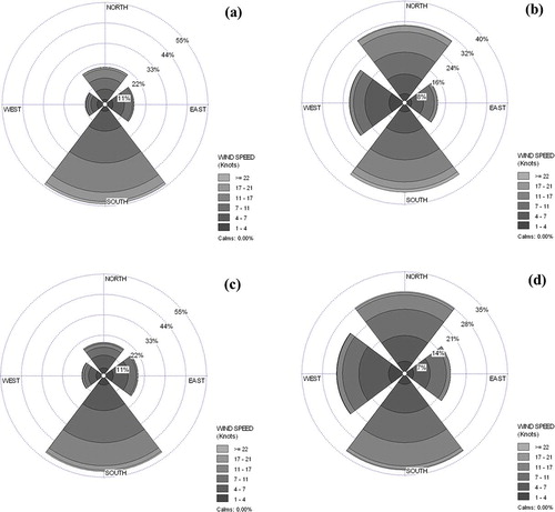
During the study period (January 2007 to December 2008), 44% and 41% of the measurements at KS1 and KS2, respectively, had wind direction from the south (135° to 225°); 23% and 21% of the measurement had wind direction from the north (0° to 45°, 315° to 360°) at KS1 and KS2, respectively. Wind usually came from the south, particularly during the months of May to November (Figure 2). Nonparametric tests indicated that the two feedlots did not significantly differ in temperature (P = 0.34) but differed significantly (P < 0.05) in wind speed.

Figure 2. Wind speed and wind direction distributions at the feedlots for the 2-yr period: (a) KS1 May to November; (b) KS1 December to April; (c) KS2 May to November; (d) KS2 December to April.

For each feedlot, measured PM₁₀ concentrations varied diurnally. Figure 3 plots the hourly concentrations for the two feedlots. The two feedlots showed similar diurnal trends: concentrations were generally lowest during the early morning period (2:00 a.m.–7:00 a.m.) and generally highest between 5:00 p.m. and 11:00 p.m.—in this study, this period was referred to as evening dust peak (EDP) period. The PM₁₀ concentrations are summarized in Table 2 as medians of hourly concentrations for the EDP and non-EDP (12:00 a.m.–4:00 p.m.) periods. Comparison of the two feedlots indicated that 24-hr PM₁₀ concentrations at KS1 and KS2 were not significantly different (P = 0.10). Comparing non-EDP and EDP periods for each feedlot, the EDP period had significantly (P < 0.001) higher concentration. These higher concentrations could be attributed to the high emission rate possibly due to high cattle activity (Mitloehner, 2000), low wind speed, and relatively stable atmospheric conditions during the EDP period (Auvermann et al., 2006).

Table 2. Median PM₁₀ concentrations at feedlot KS1 and KS2 for 2007 and 2008

	Feedlot KS1		Feedlot KS2
	12 a.m.–4 p.m.	5 p.m.–11 p.m.(EDP)	12 a.m.–4 p.m.	5 p.m.–11 p.m.(EDP)
Number of hourly values	4376	2066	3751	1607
Downwind concentration (μg/m^3)	49	82	38	53
Upwind concentration (μg/m^3)	23	27	13	17
Net concentration (μg/m^3)	32	47	22	37
Note: For each feedlot (i.e., KS1, KS2) and location (i.e., downwind, upwind, net), median concentration values for the 12 a.m.–4 p.m. and 5 p.m.–11 p.m. periods are not significantly different at the 5% level of significance.

Figure 3. Median hourly net PM₁₀ concentrations for feedlots (a) KS1 and (b) KS2. Median values were based on days with emission data. Error bars represent upper standard deviation estimates.

For the sampling days with at least 18 hourly PM₁₀ concentration measurements, measured downwind concentrations exceeded U.S. EPA National Ambient Air Quality Standards (NAAQS) for PM₁₀ (150 μg/m³ for 24-hr) (U.S. Environmental Protection Agency, 2008b) 51 (out of 74) times in 2007 and 33 (out of 71) times in 2008 for KS1 and 19 (out of 62) times in 2007 and 14 (out of 50) times in 2008 for KS2; if contribution of background (upwind) concentration was considered, the numbers of days in which the net concentrations exceeded the U.S. EPA NAAQS were fewer by 2–8 days. Higher nonattainment for KS1 could be explained by the difference in sampler location; as mentioned earlier, the sampler was closer to the pens at KS1 than at KS2. At the property lines, few hundred meters away from the pens, PM₁₀ concentrations would likely be smaller than the PM₁₀ NAAQS because of particle dispersion and settling.

Emission rates

The two feedlots differed significantly (P = 0.04) in daily emission fluxes for the 2-yr period (Table 3), with KS1 having higher emission fluxes. In 2007, median PM₁₀ emission fluxes were 1.68 g/m²-day (101 days) and 1.08 g/m²-day (91 days) for KS1 and KS2, respectively; in 2008, median PM₁₀ emission fluxes were 1.58 g/m²-day (140 days) for KS1 and 1.13 g/m²-day (95 days) for KS2. Overall median emission fluxes were 1.60 g/m²-day for KS1 and 1.10 g/m²-day for KS2. Note that KS1 had a water sprinkler system for dust control and was expected to have smaller emission rate than KS2, which did not have any sprinkler water application. However, as stated earlier, pens were cleaned more frequently at KS2 than at KS1. In addition, KS2 received more rain than KS1 (Table 1); during the 2-yr period, for KS1, 20% of the days with measurements had rainfall events; for KS2, on the other hand, 26% of the days with measurements received rainfall.

Table 3. PM₁₀ emission fluxes and factors at feedlots KS1 and KS2

		Emission Flux(g/m^2-day)		Emission Factor(kg/1000 hd-day)
Year	Parameters	KS1	KS2	KS1	KS2
January to December 2007	Number of Daily Values	101	91	101	91
	Minimum	0.04	0.09	1	2
	Maximum	9.70	6.84	162	187
	Median	1.68	1.08	28	30
January to December 2008	Number of Daily Values	140	95	140	95
	Minimum	0.07	0.06	1	2
	Maximum	9.04	6.86	151	188
	Median	1.58	1.13	26	31
Overall	Minimum	0.04	0.06	1	2
	Maximum	9.70	6.86	162	188
	Median	1.60^a	1.10^b	27^c	30^c
Note: Overall median emission fluxes or emission factors followed by the same letters are not significantly different at the 5% level of significance.

Equivalent PM₁₀ emission factors for the 2-yr period were 27 and 30 kg/1000 hd-day for KS1 and KS2, respectively (Table 3). Unlike emission fluxes, the two feedlots did not differ significantly (P = 0.53) in emission factors. The computed emission factors for both feedlots were smaller than the U.S. EPA PM₁₀ emission factor (82 kg/1000 hd-day) but were within the range of published values (Countess Environmental, 2006; McGinn et al., 2010; Wanjura et al., 2004). Compared to other studies (Countess Environmental, 2006; McGinn et al., 2010; Wanjura et al., 2004), difference in calculated emission rates could be due to differences in measurement design (e.g., measurement period) and methods (e.g., samplers), measurement conditions (e.g., time of year, weather), meteorological data set (e.g., instrument, type), emission rate estimation technique (e.g., dispersion model), and feedlot characteristics (e.g., location, pen surface conditions).

Monthly emission rates are plotted with monthly average temperatures and monthly cumulative rain amounts in Figures 4a to 4d. Monthly consumption of water for the sprinkler system operation is also shown in Figure 4e. Statistical analysis showed that the temperature significantly (P < 0.05 for KS1and KS2) affected the emission rate, whereas rainfall amount (P = 0.47 for KS1, P = 0.77 for KS2) and number of days with rainfall events (P = 0.14 for KS1, P = 0.71 for KS2) did not. Further analysis of the data for the May to November period (i.e., months with highest temperatures; 20 ± 9 °C for KS1, 21 ± 8 °C for KS2), however, revealed that the number of days with rainfall events significantly (P = 0.03) influenced emission fluxes for feedlot KS1. The May to November period had relatively higher emission rates (2.55 ± 3.66 g/m²-day for KS1, 2.35 ± 1.82 g/m²-day for KS2) than the December to April period (0.43 ± 1.32 g/m²-day for KS1, 0.50 ± 0.57 g/m²-day for KS2), which had lower temperatures (2 ± 10 °C). This was expected since high temperatures should result in high evaporation of water from pen surfaces and consequently, dryer pen surfaces, which would then have higher PM emission potential (Miller and Berry, 2005; Razote et al., 2006). Cool months, with temperatures several degrees above freezing, could still have high emission rates. An example would be the month of November in 2007. Even with low temperature (6 ± 9 °C), it had an emission flux of 4.62 g/m²-day. This emission flux was close to that of the month of August, which was the hottest month (27 ± 7 °C) and had the highest emission flux (5.69 g/m²-day) for the year. High emission rates for the month of November could be due to prolonged dry periods; during this month, KS1 only had 0.25 mm (1 day) of precipitation and the sprinkler system was not used.

Figure 4. Monthly trends of emission flux plotted with temperature at feedlots (a) KS1 and (b) KS2; with amount of rain at (c) KS1 and (d) KS2; and with amount of sprinkler water at (e) KS1.

Hourly PM₁₀ emission fluxes for KS1 and KS2 are shown in Figure 5. Highest PM₁₀ concentrations of the day were measured during the EDP period for both KS1 (47 ± 243 μg/m³) and KS2 (34 ± 125 μg/m³). Relatively high concentrations can be brought about by three conditions: high emission rate, low wind speed, and/or stable atmosphere (Cimorelli et al., 2004). All these conditions were observed at the feedlots during the EDP period: (1) computed PM₁₀ emission fluxes were relatively high during the EDP period for KS1 (16 ± 68 μg/m²-sec) and KS2 (11 ± 38 μg/m²-sec), specifically from 8:00 p.m. to 10:00 p.m.; (2) wind speed generally started to decrease around early evening (KS1: 3.5 ± 2.8 m/sec; KS2: 3.0 ± 2.2 m/sec); and (3) atmospheric conditions were generally stable during the EDP period based on the Monin-Obukhov length and on the classification by Seinfeld and Pandis (2006). High PM₁₀ emission fluxes during this period were also calculated by McGinn et al. (2010) using a non-Gaussian model (i.e., Lagrangian stochastic model). Although increase in emission rate was observed for both feedlots during the EDP period, emission fluxes at KS2 were relatively lower than at KS1. The degree of increase in emission rate could be affected by several factors such as PM control methods implemented (i.e., sprinkler system, pen cleaning) and management practice (i.e., stocking density). Even with a water sprinkler system, feedlot KS1 still had a higher emission flux than KS2, a nonsprinkled feedlot, possibly due to the greater amount of manure on the pen surface associated with less frequent pen cleaning/manure hauling at KS1. Water application would lower PM emission rate as shown previously for rainfall events; however, removal of manure from pen surfaces could also be effective in lowering PM emissions from feedlots.

Figure 5. Median hourly PM₁₀ emission fluxes at feedlots (a) KS1 and (b) KS2. Median values were based on days with emission data. Error bars represent upper standard deviation estimates.

For the late morning and afternoon periods (10:00 a.m.–5:00 p.m.), relatively lower PM₁₀ concentrations (39 ± 95 μg/m³ for KS1, 38 ± 79 μg/m³ for KS2) were measured at the two feedlots. From dispersion modeling, PM₁₀ emission fluxes were generally high during this period (27 ± 66 μg/m²-sec for KS1 and 27 ± 59 μg/m²-sec for KS2). For KS2, highest emission fluxes in the day were from this period. This high emission flux at KS2 could be due to feedlot setup and activities. However, even with high PM₁₀ emission fluxes in the afternoon period, PM₁₀ concentrations were relatively low possibly because of unstable atmospheric conditions and higher wind speeds (KS1: 4.8 ± 2.9 m/sec; KS2: 4.0 ± 2.4 m/sec).

Figure 6 plots the mean percentage contribution of each hour to the daily PM₁₀ emission flux. For KS1, the afternoon period had the highest contribution (average of 61%) to the overall daily PM₁₀ emission flux; the same was observed for KS2 (average of 66%). Average contributions of EDP period to the overall daily emission flux were 32% and 25% for KS1 and KS2, respectively. Still, emission flux for the EDP period was observed to increase during 8:00 p.m. to 10:00 p.m. period when the PM₁₀ concentration reached its peak. For days with at least 18 hourly PM₁₀ emission fluxes, nonparametric tests showed that emission fluxes during the afternoon period were significantly higher (P < 0.001 for KS1 and KS2) than those for the EDP period.

Figure 6. Percentage contribution of each hour to the daily PM₁₀ emission flux for feedlots KS1 and KS2 based on mean hourly PM₁₀ emission fluxes for the 2-yr period using days with emission data.

There were several limitations in this study that relate to PM monitoring and inherent weaknesses of atmospheric dispersion modeling. One limitation was the assumption that the emission flux was uniform throughout the feedlot and that the mass concentration, particularly on the downwind side of the feedlot, was also uniform so that a single point measurement of the concentration with a TEOM would be adequate. Another limitation is related to the atmospheric dispersion model (Holmes and Morawska, 2006; Turner and Schulze, 2007). Some studies (Faulkner et al., 2007; Hall et al., 2002) have suggested that dispersion modeling results were model specific. In addition, due to limitations of on-site weather stations, atmospheric stability (i.e., Monin-Obukhov length) was obtained from a meteorological instrumentation tower located almost 50 km away from one of the feedlots. Despite these limitations, the emission rates presented here could serve as basis for estimating emission rates for cattle feedlots and for evaluating abatement measures.

Conclusions

PM₁₀ emission rates at two cattle feedlots (KS1 and KS2) in Kansas were determined from measured TEOM PM₁₀ concentrations using inverse dispersion modeling with AERMOD. For the 2-yr period, daily average PM₁₀ concentration downwind exceeded 150 μg/m³ 84 out of 145 days for KS1 (downwind locations of 5 and 30 m) and 33 out of 112 days for KS2 (downwind locations of 40 and 60 m) for days with at least 18 hourly concentration measurements. Based on the 2-yr study period, feedlot KS1, equipped with a sprinkler system, had a median PM₁₀ emission flux of 1.60 g/m²-day (241 days) and emission factor of 27 kg/1000 hd-day. KS2, a nonsprinkled feedlot but with more frequent pen cleaning, had a median PM₁₀ emission flux of 1.10 g/m²-day (186 days) and emission factor of 30 kg/1000 hd-day. These emission factors were considerably smaller than published EPA PM₁₀ emission factor for cattle feedlots.

Emission fluxes were greater during warm season and prolonged dry periods, generally because of the presence of dry, uncompacted manure layer on pen surfaces. Hourly emission rates varied during a given day. Highest emission fluxes were observed for the 10:00 a.m. to 5:00 p.m. period; possibly because of unstable atmospheric conditions, however, measured PM₁₀ concentration during this period was not high. Emission flux also increased in the evening from 8:00 p.m. to 9:00 p.m., possibly due to greater animal activity during this period. Due to stable atmospheric conditions, very high PM₁₀ concentration was measured for this period.

Acknowledgments

This study was supported by U.S. Department of Agriculture (USDA) National Institute of Food and Agriculture Special Research Grant “Air Quality: Reducing Air Emissions from Cattle Feedlots and Dairies (TX and KS)” through the Texas AgriLife Research and by Kansas Agricultural Experiment Station. Some of the meteorological data were obtained from the Atmospheric Radiation Measurement (ARM) Program sponsored by the U.S. Department of Energy, Office of Science, Office of Biological and Environmental Research, Climate and Environmental Sciences Division. Technical assistance provided by Darrell Oard, Dr. Jasper Tallada, Dr. Li Guo, Kevin Hamilton, and Howell Gonzales of Kansas State University; Sheraz Gill of San Joaquin Valley Air Pollution Control District; and Dr. James Thurman of EPA is acknowledged. Cooperation of feedlot operators and KLA Environmental Services, Inc., is also acknowledged.

References

- Auvermann , B , Bottcher , R. , Heber , A. , Meyer , D. , Parnell , C.B. Jr. , Shaw , B. and Worley , J. 2006 . “ Particulate matter emissions from animal feeding operations ” . In Animal Agriculture and the Environment: National Center for Manure and Animal Waste Management White Papers , Edited by: Rice , J.M. , Caldwell , D.F. and Humenik , F.J. St. Joseph : ASABE .
- Baum , K.A. 2003 . Air emissions measurements at cattle feedlots , Edited by: thesis , M.S. Manhattan , KS : Kansas State University .
- Calder , K.L. 1977 . Multiple-source plume models of urban air pollution – their general structure . Atmosphric Environment , 11 : 403 – 414 .
- CFR . 2005 . Revision to the guideline of air quality models: adoption of a preferred general purpose (flat and complex terrain) dispersion model and other revisions . Code of Federal Regulations , Part 51 ( Title 40 )
- Cimorelli , A.J. , Perry , A. , Venkatram , A. , Weil , J.C. , Paine , R.J. , Wilson , R.B. , Lee , R.F. , Peters , W.D. , Brode , R.W. and Paumier , J.O. 2004 . AERMOD: Description of Model Formulation , 68218 – 68261 . Research Triangle Park , NC : U.S. Environmental Protection Agency . EPA-454/R–03–004.
- Countess Environmental . 2006 . Western Regional Air Partnership (WRAP) Fugitive Dust Handbook , Denver : Western Governors’ Association . Contract No. 30204-111
- Faulkner , W.B. , Goodrich , L.B. , Botlaguduru , V.S.V. , Capareda , S.C. and Parnell , C.B. 2009 . Particulate matter emission factors for almond harvest as a function of harvester speed . Journal of the Air and Waste Management Association , 59 : 943 – 949 . doi: 10.3155/1047–3289.59.8.943
- Faulkner , W.B. , Powell , J.J. , Lange , J.M. , Shaw , B.W. , Lacey , R.E. and Parnell , C.B. 2007 . Comparison of dispersion models for ammonia emissions from a ground-level area source . Transactions of the ASABE , 50 : 2189 – 2197 .
- Gonzales , H. 2010 . Particulate emissions from cattle feedlots – particle size distribution and contribution of wind erosion and unpaved roads , Edited by: thesis , M.S. Manhattan , KS : Kansas State University .
- Goodrich , L.B. , Faulkner , W.B. , Capareda , S.C. , Krauter , C. and Parnell , C.B. 2009 . Particulate matter emissions from reduced-pass almond sweeping . Transactions of the ASABE , 52 : 1669 – 1675 .
- Grelinger , M.A. and Lapp , T. An evaluation of published emission factors for cattle feedlots . Proceedings of International Conference on Air Pollution from Agricultural Operations . 1996 , Kansas City , MO . February . pp. 7 – 9 . Ames , IA : MidWest Plan Service .
- Hall , D.J. , Spanton , A.M. , Bennett , M. , Dunkerley , F. , Griffiths , R.F. , Fisher , B.E.A. and Timmis , R.J. 2002 . Evaluation of new generation atmospheric dispersion models . International Journal of Environment and Pollution , 18 : 22 – 32 .
- Holmes , N.S. and Morawska , L. 2006 . A review of dispersion modeling and its application to the dispersion of particles: an overview of different dispersion models available . Atmospheric Environment , 40 : 5902 – 5928 . doi: 10.1016/j.atmosenv.2006.06.003
- MACTEC Federal Programs, Inc . 2009 . Addendum – User's guide for the AMS/EPA Regulatory Model – AERMOD , Manhattan , KS : U.S. Environmental Protection Agency . EPA-454/B-03-001
- McGinn , S.M. , Flesch , T.K. , Chen , D. , Crenna , B. , Denmead , O.T. , Naylor , T. and Rowell , D. 2010 . Coarse particulate matter emissions from cattle feedlots in Australia . Journal of Environmental Quality , 39 : 791 – 798 . doi: 10.2134/jeq2009.0240
- Midwest Research Institute . 1988 . Gap Filling PM10 Emission Factors for Selected Open Area Dust Sources , Research Triangle Park : U.S. Environmental Protection Agency . EPA-450/4–88–003
- Miller , D.N. and Berry , E.D. 2005 . Cattle feedlot soil moisture and manure content: I. Impacts on greenhouse gases, odor compounds, nitrogen losses, and dust . Journal of Environmental Quality , 34 : 644 – 655 .
- Mitloehner , F.M. 2000 . Behavioral and environmental management of feedlot cattle , Lubbock , TX : Texas Tech University . Ph.D. dissertation
- National Research Council . 2003 . Air Emissions from Animal Feeding Operations: Current Knowledge, Future Needs , Washington : National Academy of Sciences .
- Pacific Environmental Services, Inc . 1995 . User's Guide for the Industrial Source Complex (ISC3) Dispersion Models , Research Triangle Park : U.S. Environmental Protection Agency . EPA-454/B-95-003b
- Pacific Environmental Services, Inc . 2004 . User's Guide for the AMS/EPA Regulatory Model – AERMOD , Research Triangle Park : U.S. Environmental Protection Agency . EPA-454/B-03-001
- Perry , S.G. , Cimorelli , A.J. , Paine , R.J. , Brode , R.W. , Weil , J.C. , Venkatram , A. , Wilson , R.B. , Lee , R.F. and Peters , W.D. 2005 . AERMOD: a dispersion model for industrial source applications. Part II: model performance Against 17 field study databases . Journal of Applied Meteorology , 44 : 694 – 708 .
- Purdue Applied Meteorology Laboratory . 2009 . Quality Assurance Project Plan for the National Air Emissions Monitoring Study, Revision No. 3 , West Lafayette : Purdue University .
- Razote , E.B. , Maghirang , R.G. , Predicala , B.Z. , Murphy , J.P. , Auvermann , B.W. , Harner , J.P. and Hargrove , W.L. 2006 . Laboratory evaluation of the dust emission potential of cattle feedlot surfaces . Transactions of the ASABE , 49 : 1117 – 1124 .
- San Joaquin Valley Air Pollution Control District. 2006. Dairy and feedlot PM10 emission factors: draft office memo. http://www.valleyair.org/ (http://www.valleyair.org/) (Accessed: 5 March 2010 ).
- SAS Institute Inc . 2004 . SAS System for Windows, Release 9.1.3 , Cary : SAS Institute Inc .
- Schwertman , N.C. , Owens , M.A. and Adnan , R. 2004 . A simple more general boxplot method for identifying outliers . Computational Statistics and Data Analysis , 47 : 165 – 174 . doi: 10.1016/j.csda.2003.10.012
- Seinfeld , J.H. and Pandis , S.N. 2006 . Atmospheric Chemistry and Physics—From Air Pollution to Climate Change , 2nd , Hoboken : John Wiley & Sons .
- Turner , D.B. and Schulze , R.H. 2007 . Practical Guide To Atmospheric Dispersion Modeling , Dallas : Trinity Consultants, Inc. and Air & Waste Management Association .
- U.S. Department of Agriculture . 2011 . Cattle on Feed , Washington : National Agricultural Statistics Service, U.S. Department of Agriculture .
- U.S. Environmental Protection Agency . 2001 . Procedures Document for National Emission Inventory, Criteria Air Pollutants 1985–1999 , Research Triangle Park : U.S. Environmental Protection Agency . EPA-454/R–01–006
- U.S. Environmental Protection Agency . 2003 . National Air Quality and Emissions Trends Report – 2003 Special Studies Edition , Research Triangle Park : U.S. Environmental Protection Agency . EPA-454/R–03–005
- U.S. Environmental Protection Agency . 2008a . AERSURFACE User's Guide , Research Triangle Park : U.S. Environmental Protection Agency . EPA-454/B-08-001
- U.S. Environmental Protection Agency . 2008b . Integrated Review Plan for the National Ambient Air Quality Standards for Particulate Matter , Research Triangle Park : U.S. Environmental Protection Agency . EPA-452/R-08-004
- U.S. Environmental Protection Agency . 2009 . AERMOD Deposition Algorithms – Science Document (Revised Draft) , Research Triangle Park : U.S. Environmental Protection Agency .
- Wanjura , J.D. , Parnell , C.B. , Shaw , B.W. and Lacey , R.E. A Protocol for determining a fugitive dust emission factor from a ground level area source . American Society of Agricultural Engineers (ASAE) Proceedings . August 2004 , Ontario , Canada. pp. 1 – 4 . St. Joseph : ASAE . Paper 044018