Using pseudometrics in kernel density estimation

Abstract

Common kernel density estimators (KDE) are generalised, which involve that assumptions on the kernel of the distribution can be given. Instead of using metrics as input to the kernels, the new estimators use parameterisable pseudometrics. In general, the volumes of the balls in pseudometric spaces are dependent on both the radius and the location of the centre. To enable constant smoothing, the volumes of the balls need to be calculated and analytical expressions are preferred for computational reasons. Two suitable parametric families of pseudometrics are identified. One of them has common KDE as special cases. In a few experiments, the proposed estimators show increased statistical power when proper assumptions are made. As a consequence, this paper describes an approach, where partial knowledge about the distribution can be used effectively. Furthermore, it is suggested that the new estimators are adequate for statistical learning algorithms such as regression and classification.

Keywords:

• nonparametric density estimation
• semiparametric density estimation
• nonparametric regression
• nonparametric functional data analysis
• volume of ball in pseudometric space

Introduction

The multivariate kernel density estimator (KDE) with a fixed bandwidth is given by

(1)

where is a single modal, symmetric, nonnegative and zero-mean function that integrates to 1. The bandwidth matrix describes the level of smoothing. It is convenient to write , where h is a positive scalar and . With this parametrisation, the shape is determined by and the scale is determined by h. This gives

(2)

where K is a kernel that is independent of . The first univariate version of Equation (2) was proposed by Fix and Hodges (1951), while the general class was investigated by Rosenblatt (1956) and Parzen (1962). The multivariate extension was outlined by Cacoullos (1966) and Epanechnikov (1969).

Several authors have suggested a variable bandwidth version of Equation (2), where the two main approaches are the balloon estimator and the sample smoothing estimator. A comparison between KDE with fixed and variable estimators is given by Terrel and Scott (1992).

The balloon estimator lets to be equal to the distance to the kth nearest neighbour of . The estimator is given by

(3)

The first version of this estimator was published by Loftsgaarden and Quesenberry (1965) and has later been known as the k-nearest neighbour estimator. It is given by

(4)

where n is the sample size, V_m the volume of the m-dimensional Euclidean unit ball and r the Euclidean distance between and its kth nearest neighbour. Equation (4) can be derived from Equation (3), if we choose to be identity and a kernel that is a uniform density on the m-dimensional Euclidean unit ball. In Loftsgaarden and Quesenberry (1965), it was also proved that the estimator in Equation (4) is consistent for increasing n.

The sample smoothing estimator was suggested by Breiman, Meisel, and Purcell (1977). Here, the bandwidth parameter is independent of the query point, but dependent on the sample points. The estimator is where is the distance to the k-nearest neighbour of .

To improve readability, we recollect the following definitions.

Definition 1.1

The kernel of a function is an equivalence relation =_f given by where and are elements in X.

Definition 1.2

A pseudometric on a set X is a function (distance function) which for all in X satisfies the following conditions:

• 1.  (non-negativity ).

• ] (symmetry ).

• ] (triangle inequality).

If we add the requirement of identity, which is if and only if then d is a metric as well.

Definition 1.3

A pseudometric space M is an ordered pair (X, d). A closed ε- ball on M that is centred at is defined as which is equivalent to the definition of a closed ε-ball in a metric space. Note that ε is called the radius of the ball.

This definition of pseudometric is exactly the same as the definition of a semimetric in the field of nonparametric functional data analysis (Ferraty and Vieu 2006). To avoid confusion in this paper, we will keep referring to pseudometrics, even though most of the literature in nonparametric functional data analysis uses the term semimetric.

In nonparametric functional data analysis, the explanatory variables are functional and most of the work has been done on regression and classification. An overview of the field is given in the book by Ferraty and Vieu (2006). In the case of density estimation, Delaigle and Hall (2010) proved that a probability density function generally does not exist for functional data, but developed notions of density and mode, when functional data are considered in the space determined by the eigenfunctions of the principal components. In the paper by Ferraty, Kudraszow, and Vieu (2012), an infinite dimensional analogue of a density estimator is discussed, when the small ball probability associated with the functional data can be approximated as a product of two independent functions; one depending on the centre of the ball and one depending on the radius.

In this paper, we consider only finite dimensional pseudometric spaces, where balls with finite radius have finite volumes. Such spaces exist as a specification of the theory of nonparametric functional data analysis (Ferraty et al. 2012). The theory in this paper is distinguished from that of nonparametric functional data analysis, because we consider pseudometric spaces, where volumes of balls with fixed radius are allowed to be dependent on locations of centres. In all previous work on using pseudometrics for functional data, the volumes of the balls are always considered as independent on the locations of the centres. This generalisation opens up for applications that are less linked to functional data and more related to restricted nonparametric and semiparametric estimators on real (non-functional) data.

To be more accurate, the parameters of the pseudometric precisely describe the kernel, or more roughly the level sets of the distribution. This is important for visualisation and interpretation of the estimated distribution. For instance, the complete multi-dimensional density that is estimated with an estimator using a pseudometric of family one (described later in this paper) can be described by a two-dimensional plot only.

The choice of the family of pseudometrics describes the constraints on the level sets of the distributions that can be modelled. In case of fitting parameters, it is therefore important that the level sets of the actual distribution are not in violation with these constraints. This is somewhat analogous to parametric models, where serious misbehaviour can be observed, if the distribution has a different shape than any of the members in the family of models.

An example of a similar approach can be found in a paper by Liescher (2005), where the level sets of the distributions were constrained to be of elliptic shape. The elliptic shape of the level sets was constrained by a transformation that was performed prior to applying the nonparametric density estimator. It was shown that the convergence rates were independent of the number of dimensions, except in the neighbourhood of the mean, and thereby overcoming the so-called curse of dimensionality. The estimators in this paper can be seen as a generalisation of the estimators of Liescher (2005), because a wider family of associated distributions is allowed. Convergence rates are not explicitly given in this paper, but simulations show that the performance close to the mode coincides with the common KDE and improves quickly away from the mode, which is similar to the results obtained by Liescher (2005).

In the context of reducing the curse of dimensionality of nonparametric density estimators, it is also worth mentioning the projection pursuit density estimator. This method was first introduced in Friedman, Stuezle, and Schroeder (1984), and a parametric extension was given by Welling, Zemel, and Hinton (2003). In projection pursuit one projects the explanatory variables into principal directions and fits one-dimensional smooth density functions to these projections. The resulting density is the product of these densities. A special case is the flexible Bayesian estimator, where the projection matrix is identity. In essence, the flexible Bayesian method is assuming independence between the explanatory variables. The estimator will be used later in this paper and is plug-in where K is a univariate kernel, the bandwidth is h, x_j is the jth coordinate of and x_ij is the jth coordinate in sample i. Consistency is proved under the assumption of independence (John and Langley 1995). This is a nonparametric variation of the old and well-known naive-Bayesian estimator, where the individual distributions are assumed Gaussian. A similarity between the estimators in this paper and the projection pursuit density estimators is that the resulting density can be visualised in lower dimensional spaces. In projection pursuit, it is enough to show the one-dimensional (ridge) functions along with the principal directions to understand the full distribution.

The proposed estimators have less in common with semiparametric models, where part of the model is fully parametric. For instance models which are a product of a parametric and a nonparametric component, such as in Naito (2004) and references therein. Another example is when some of the explanatory variables are modelled nonparametrically, while the rest are modelled parametrically, such as in Hoti and Holmström (2003).

In the next section, the underlying assumptions of the KDE with fixed and variable bandwidths are discussed. This is followed by formal definitions of the new estimators. A framework for finding suitable parametric families of pseudometrics is outlined in Section 3 and two families are identified. Some experiments are given in Section 4, where the new KDE are compared with common KDE on samples drawn from common distributions. In Section 5, open questions and ideas of how to use the new estimators on various problems are elaborated on, before the work is concluded.

2. Assumptions for kernel density estimation and definition of new estimators

It is convenient to start our discussion by investigating the k-nearest neighbour method, because it is conceptually easier than the other KDE. If we generalise Equation (4) for using any metric d, then

(5)

where is the kth nearest neighbour of and is the volume of the ball in the metric space with radius .

For the sake of discussion, a random variable Y is defined as a k-nearest neighbour estimate at a particular . Each k-nearest neighbour estimate requires drawing a new training sample and this is why Y is a random variable. The variance of Y is a consequence of which sample is chosen (because this determines the location of the kth-nearest neighbour), while a great portion of the bias can be explained by the shape of the ball.

This is potentially more clear if we realise that Equation (5) can be derived from two assumptions that were not stated in Loftsgaarden and Quesenberry (1965). The first assumption is that

(6)

The second assumption is that is equal to the mean of inside , because the left-hand side of Equation (6) is equal to , which is how Equation (6) implies Equations (5) and (4). A measure for how much the second assumption is violated is identified as

(7)

The parameter AV is therefore highly dependent on which metric is chosen, because the metric determines the shape and the size of the region of integration. A great portion of the bias of Y is a consequence of the second assumption. Also, we recognise that there is a connection between f and the choice of metric. No metric is optimal for any f and vice versa.

This argumentation can be transferred to all KDE with both fixed and variable bandwidths, because these methods are essentially weighting the contribution of each sample as a function of . For the KDE with fixed bandwidth, the balloon estimator and the sample smoothing estimator, respectively, we could write where , and are nonnegative, strictly decreasing, one-sided univariate kernels that integrate to one, when integrated over . If we let the random variable Y be defined as any of the kernel density estimates at a particular , then the bias of Y is highly related to the shape of the balls in combination with the shape of the f near .

2.1. Definition of the k-nearest pseudo-neighbour estimator

A generalisation of the k-nearest neighbour estimator is proposed as where d_p is a pseudometric. Figure 1 illustrates the principles of k-nearest neighbour estimator as of Loftsgaarden and Quesenberry (1965) together with the k-nearest pseudo-neighbour estimator. This particular pseudometric is a special case of the parametric families of pseudometrics that are outlined later in this paper.

Figure 1. Description of the k-nearest pseudo-neighbour estimator. The scatter plot shows a training population with 100 points that are i.i.d and drawn from a two-dimensional normal distribution. A cross is marked at a query point and in k-nearest neighbour estimation, the kth-nearest neighbour is found by comparing the Euclidean distance to all other points. The smallest Euclidean ball that encapsulates the 5th-nearest neighbours is shown as a solid circle. Clearly, f is not very constant inside this ball. In k-nearest pseudo-neighbour estimation, the kth-nearest neighbour is found by comparing the distance in the pseudometric space from the query point to all other points. The interior between the two dashed lines represents a ball in this pseudometric space, where the query point is in the centre. The radius of the ball (not of the dashed circles) is the distance to the 5th-pseudo-nearest neighbour. Obviously, f is far more constant inside this ball. Consequently, improved statistical power is achieved when the equivalence classes with respect to the kernel of the distribution are assumed to be circles around the mean.

It is postulated that a proper choice of a pseudometric can reduce Equation (7) far more than a metric, because balls in pseudometric spaces span a richer variety of shapes. The key idea is to find a parametric family of pseudometrics and select parameters by either Bayesian inference or learning.

It is a crucial point that the parameters of a pseudometric family are typically associated with various sample statistics and associations between the explanatory variables. In the example shown in Figure 1, the centre of the dashed circles is a parameter of the pseudometric. This parameter can be estimated by the sample mean.

2.2. Definition of pseudometric KDE

A challenge with using pseudometrics is that the volumes of the balls with constant radius are generally dependent on the locations of the centres. This effect is neutralised by defining the equivalent Euclidean distance, which is the function

(8)

where V_m is the volume of the Euclidean unit m-ball. The equivalent Euclidean distance from to in a pseudometric space is the radius of the Euclidean m-ball that has the same volume as . Note that is generally not a metric, nor a pseudometric, because the symmetry criteria are broken.

The idea is to weight the contributions of the ’s according to the equivalent Euclidean distances from the query point. This ensures that the level of smoothing is constant with respect to volume, which is the case for KDE with fixed bandwidths.

The pseudometric kernel density estimator (PKDE) is suggested as

(9)

where K_h(u) is the kernel with bandwidth h and is equal to 1/n at the s and 0 elsewhere. An example of a kernel is the one-dimensional normal, which is given by This is realised because integrates to 1, when integrated over u. Notice that the kernel itself is not dependent on the choice of pseudometric. Only the number of dimensions is necessary input.

If we choose where and a bandwidth h, then Equation (1) becomes a special case of Equation (9), when and normal kernels are used. The only difference is that the kernel in Equation (9) takes a scalar argument, while the kernel in Equation (1) takes a vector. A similar argumentation can be made for any kernel and this is why the PKDE is a generalisation of the standard KDE.

In the case of variable bandwidths, the pseudometric balloon estimator is suggested as where and is the k-nearest pseudo-neighbour of (nearest in the sense d_p). Notice that if we choose d_p to be Euclidean and a kernel that has uniform density on the Euclidean ball, the k-nearest neighbour method falls out as a special case.

Moreover, the pseudometric sample smoothing estimator is suggested as where and is the k-nearest pseudo-neighbour of .

3. Choosing appropriate parametric families of pseudometrics

A clear challenge with using the new estimators is proposing suitable families of pseudometrics. It is therefore instructive to define the equivalence relation , where if and only if . While discussing the usefulness of a family of pseudometrics, it makes sense to ask which density functions are invariant to , and the next two definitions are motivated by this.

Definition 3.1

A probability density function is said to be an associated distribution of a pseudometric (or metric) d_p, denoted as when is invariant to . Invariance to means that implies that for all in X.

Definition 3.2

An associated distribution satisfies the strong condition if is equal to where is the kernel of . This is the case when for all in X.

3.1. Volumes of generalised balls

Two new families of pseudometrics are proposed, including the associated distributions and the derivations of the analytical expressions for the volumes of their balls. Before this, a definition of the closed linearly transformed generalised balls and a derivation of an analytical expression for the volumes are needed. Table 1 contains a list of symbols that are consistently used in rest of this paper.

Table 1. List of important symbols.

Symbol	Explanation and properties
m	Number of dimensions
m1, m2	Used in pseudometric , where m1 and m2 are nonzero integers and m1+m2=m
	Linear transformation matrix of size m×m, where
	Centre point parameter (not centre of the balls). Size is either m or m1 depending on the context
	Vector of positive exponents in pseudometrics. Size is either m or m1 depending on the context
p	Harmonic average of the elements in
q	Exponent that is used in pseudometric
	Identity matrix with size m×m or
	Null vector with size m, m1 or m2
	Centre point of the balls. Length is m
ε	Radius of the balls. ε>0
	Volume of the generalised unit ball with parameter

Definition 3.3

The closed linearly transformed generalised ε-ball that is centred in is denoted where Here, is a vector of the positive p_is, while p is the harmonic average of the p_i′s (i.e. ). Moreover, and where A is a square transformation matrix with nonzero determinant.

In general is a semimetric, because the triangle inequality does not hold when at least one of the p_is are less than 1. Depending on the p_is, the generalised balls describe a wide range of multi-dimensional geometrical objects, where spheres, cubes, cylinders and stars are special cases. A few three-dimensional objects are shown in Figure 2.

Figure 2. Generalised unit balls. (a) , (b) and (c) .

In articles by Wang (2005) and Gao (2013), the volume of the generalised unit ball was derived.

Theorem 3.4

The volume of the closed generalised unit ball is

(10)

where I is the identity matrix.

The proof by Wang used induction and was motivated by an idea from Folland (2001), while the proof by Gao used properties of the exponential distribution. An alternative proof of Equation (10) is included in the appendix.

Theorem 3.5

The volume of the closed linearly transformed generalised ε-ball that is centred in is

This means that and the absolute value of the determinant of determine the overall scaling of the volume. This is a consequence of choosing the exponent in to be 1/p.

3.2. Pseudometric family of type one

Definition 3.6

The pseudometric family of type one is given by where is a chosen point (for instance a mean or a median).

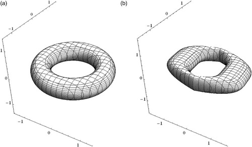
The parameters that can be trained for this pseudometric are , and . In the family of pseudometric spaces (), the balls can be viewed as generalisations of the spherical shell and two examples are shown in Figure 3.

Figure 3. Balls in the pseudometric spaces (ℝ³, d_{p1, I, 0, p}). One octant is removed in both figures, so it is possible to see more of the boundaries of the balls. (a) and (b) .

3.2.1. Associated distributions

Theorem 3.7

The family of associated distributions is equal to a function g(u), which satisfies

(11)

where u = . Moreover, satisfies the strong condition.

If we choose g(u) to be an exponential function a exp(−u), then the coefficient a can be found from Equation (11). When inserting for g(u), the integral part of Equation (11) becomes , so that

The parametric family of associated distributions is therefore a linear transformation of the m-dimensional generalised normal distribution (also known as the exponential power distribution)

To interpret this result, a description of the univariate case is given by where more details are given in Figure 4. Also, if we choose to be diagonal with 1/α_is on the diagonal then In this case all dimensions are independent and the α_is are the scale factors and p_is are the shape factors.

Figure 4. The univariate generalised normal distribution is a parametric family of symmetric unimodal distributions that includes all normal and Laplace distributions, and as limiting cases it includes all continuous uniform distributions on bounded intervals of the real line. It includes a shape factor β and a scale factor α. Various choices of shape factors are shown in this figure, where the scale factor is 1 and the mean is 0.

3.2.2. Volumes of the balls

Theorem 3.8

The volumes of the balls in the family of pseudometric spaces are given by where O is the set of positive odd numbers that are smaller than or equal to m.

The continuity of the ball at is seen, when noting the fact that and . In the case when , the volume is a polynomial with respect to either ε or . The same is true when , but the polynomial is different. This demonstrates how the volumes of the balls are dependent on the locations of the centres, and this is why it was necessary to define the equivalent Euclidean distance in Equation (8).

3.3. Pseudometric family of type two

Definition 3.9

The pseudometric family of type two is proposed as where q is an integer larger than or equal to one, I is identity, and . The notations means and is the upper left sub-matrix of A with size . Also we have m₁+m₂=m.

The parameters that can be trained here is q, , and , but also which x_is are put into (it does not have to be the m₁ first). In the limiting case when

The ball is as usual defined by If m₁ is less or equal to 1, is the familiar m-dimensional ball. The familiar torus and a deformation of a torus are other special cases that are shown in Figure 5.

Figure 5. Balls in the pseudometric spaces (ℝ³, d_{p2, I, 0, p, 2}). Here, m₁ is 2. (a) and (b) .

3.3.1. Associated distributions

In terms of discussing the associated distributions for , it is an important observation that the equivalence classes of are all topological manifolds of dimension m₁−1, while the equivalence classes of are (m−1)-manifolds. This means that can never be equal to , unless m₁ is equal to m.

This dimension reduction may be desirable with regards to improving robustness, because the family of associated distributions spans wider. On the other side, it may reduce statistical power because AV defined in Equation (7) may not be minimised properly.

Theorem 3.10

The parametric family of associated distributions is equal to a function which satisfies where .

If we also assume that the are all independent of (and vice versa), then . Hence, g₁(u) is subject to the constraint while is a probability density function that integrates to 1, when integrated over . Clearly, the family of associated distributions has the family of associated distributions and the family of all distributions as special cases.

3.3.2. Volumes of the balls

Theorem 3.11

The volumes of the balls in the family of pseudometric spaces are given by

where Here, B_t(a, b) is the incomplete beta function, and O is the set of positive odd numbers that are smaller than or equal to m₁.

In the case when , the volume is a polynomial with respect to either ε or . The same is true when , but the polynomial is different.

Theorem 3.12

The volumes of the balls in the family of pseudometric spaces in the limiting case when are given by where O is the set of positive odd numbers that are smaller than or equal to m₁.

The continuity of the ball at is seen, when noting the fact that and . This formula is simpler than the general formula given in Theorem 3.11 and it may be desirable in the context of reducing computational time.

3.4. Bandwidth selection

In Rosenblatt (1956), approximations for the bias, the variance, the mean squared error and the mean integrated squared error were derived in the univariate case. It was shown that by minimising the asymptotic mean integrated squared error (AMISE), an optimal bandwidth could be found when information of exists. It is not possible to make such an elegant argumentation for pseudometric kernel density estimation. However, an expression, including one-dimensional integrals, for the AMISE of is derived when f is equal to .

Theorem 3.13

The asymptotic mean squared error of and the AMISE of are

(12)

where and are given by

(13)

and

(14)

Here, and .

4. Experiments

In this section, a few experiments are presented where various PKDE are compared with the standard KDE and the flexible Bayesian estimator. The experiments involve drawing repetitively an order pair , n_rep times. Here, X is a sample of n points that are drawn from a known distribution f and is a query point that is drawn randomly from an equivalence class . The sequence starts at 0 and is uniformly spaced over the relevant domain of f. For every r_i, the mean and the quartiles are computed and compared with the known analytic solution. When plotted as a function of r_i, the variances and the biases of the estimators are easily seen.

Seven experiments are conducted, where PKDE, KDE and flexible Bayesian are compared on a set of distributions, including the standard normal, the uniform, the one-sided normal and a one-sided normal that is split into two. Variable PKDE and variable KDE are compared only on the standard normal distribution. The parameters are summarised in Tables 2 and 3.

Table 2. Parameters for all experiments.

Parameter	Argument
Number of repetitions nrep	10,000
Sample size n	1000
Number of equivalence classes neqc	50
Pseudometric family	Type one
Transformation matrix	Identity
Centre point

Table 3. Parameters for each experiment.

	Distribution				Exponents in
No.	type	Dimensions^a	Method	Bandwidth	pseudometric
1	Standard normal	2	PKDE	0.5	All are 2
		4
		6
2	Standard normal	6	PKDE	0.2	All are 2
		0.8
3	Standard normal	6	KDE	0.5	NA
			Flexible Bayesian	0.2
4	Standard normal	6	Variable PKDE	15th nearest neighbour	All are 2
			Variable KDE
5	Uniform on [−0.5, 0.5]	6	PKDE	0.15	All are 12
			KDE	0.15
			Flexible Bayesian	0.04
6	One-sided standard normal	6	PKDE	0.25	All are 2
			KDE	0.25
			Flexible Bayesian	0.1
7	One-sided standard normal split into two	6	PKDE	0.25	All are 2
			KDE	0.25
			Flexible Bayesian	0.1

^aNumber of dimensions.

4.1. Results

In experiment one (Figure 6), the estimator is shown in various dimensions while the bandwidth is kept constant. The bandwidth is chosen to 0.5, which is the bandwidth that minimises AMISE (12) in six dimensions. The estimator seems to be unbiased in the tails, while it underestimates near the centre where the level of underestimation increases with the number of dimensions. The tails seem fairly unbiased, but as we move away from the centre, the mean normalised experimental error starts to fluctuate. From the quartile plots, it is seen that the skewness of the normalised experimental error increases with distance from the centre.

Figure 6. Result of experiment one. Kernel density estimates for a standard normal distribution in various number of dimensions, where the bandwidth is 0.5. The top row shows the densities as functions of the distances from the centre, while the bottom row shows the corresponding normalised standard errors. The distance from the centre is chi distributed with order m and the shaded area is where the cumulative distribution function is between 0.025 and 0.975. (a) Two dimensions, (b) four dimensions and (c) six dimensions.

In experiment two (Figure 7), we see the effect of increasing and decreasing the bandwidth in six dimensions. When the bandwidth is increased, the underestimation near the centre increases while the variance decreases everywhere. When the bandwidth is decreased, the bias is reduced at the cost of a higher variance.

Figure 7. Result of experiment two. Kernel density estimates for a standard normal distribution in six dimensions with various degrees of smoothing. The top row shows the probability density functions as functions of the distances from the centre, while the bottom row shows the corresponding normalised standard errors. The distance from the centre is chi distributed with order six. The shaded area is where the cumulative distribution function is between 0.025 and 0.975. (a) Bandwidth is 0.2 and (b) bandwidth is 0.8.

In experiment three (Figure 8), KDE with fixed bandwidth and flexible Bayesian is shown for comparison with PKDE in experiment one. Since the bandwidth in KDE is the same as for PKDE, the bias and the variance are the same near the centre, while KDE continues to underestimate much further away from the centre. Also, when the analytical graph is passed, KDE starts to overestimate. Obviously, an optimal bandwidth for KDE is smaller than for PKDE, since the bias in the tail is larger. This underestimation and overestimation pattern is also seen in the flexible Bayesian, but to a lower extent. In the case of the flexible Bayesian, we have chosen a bandwidth so that the variance near the centre is approximately the same as the KDE and the PKDE. This means that it is easier to compare the biases.

Figure 8. Result of experiment three. KDE and flexible Bayesian estimates for a standard normal distribution in six dimensions, where the bandwidths are 0.5 and 0.2, respectively. The top row shows the probability density functions as functions of the distances from the centre, while the bottom row shows the corresponding normalised standard errors. The distance from the centre is chi distributed with order six. The shaded area is where the cumulative distribution function is between 0.025 and 0.975. (a) KDE and (b) flexible Bayesian.

In experiment four (Figure 9), PKDE and KDE with variable bandwidths are shown for comparison. The number of neighbours is chosen so that the variances near the centres are approximately the same as in Figures 6 and 8, where the bandwidths are fixed. It is interesting to see that the variance of the normalised experimental error is fairly stable and not skewed compared to the fixed bandwidth graphs. The bias in the tails is clear in these plots. Notice also that the PKDE with variable bandwidth has a similar, or smaller, variance and bias than the flexible Bayesian inside the shaded area.

Figure 9. Result of experiment four. Variable PKDE and variable KDE for a standard normal distribution in six dimensions. Two standard deviations of the Gaussian kernel are defined to be the distance (in the pseudometric space) to the 15th nearest neighbour. The top row shows the probability density functions as functions of the distances from the centre, while the bottom row shows the corresponding normalised standard errors. The distance from the centre is chi distributed with order six and the shaded area is where the cumulative distribution function is between 0.025 and 0.975. (a) Variable PKDE and (b) variable KDE.

In experiment five (Figure 10), PKDE, KDE and flexible Bayesian are compared on a uniform population. The bandwidth of the flexible Bayesian is adjusted so the variance near the centre is similar for all estimators. Clearly, PKDE has the sharpest border, while KDE is outperformed by the other two.

Figure 10. Result of experiment five. PKDE, KDE and flexible Bayesian on a six-dimensional uniform distribution on [−0.5, 0.5]. The bandwidth for the flexible Bayesian estimate is 0.04, while it is 0.15 for the other two. The shaded area is where the cumulative distribution function of the (pseudometric) distance to the centre is between 0.025 and 0.975. (a) PKDE, (b) KDE and (c) flexible Bayesian.

In experiment six (Figure 11), the estimators are evaluated on a one-sided normal distribution. When the bandwidth is half the bandwidth used in experiment one, PKDE performs identically to PKDE in experiment one. KDE, on the other hand, underestimates far more than in the two sided case in experiment three. This is particularly the case near the centre. The same effect is present for the flexible Bayesian.

Figure 11. Result of experiment six. PKDE, KDE and flexible Bayesian for a one-sided standard normal distribution in six dimensions, where the bandwidths are 0.1 for the flexible Bayesian estimates and 0.25 for the other methods. The top row shows the probability density functions as functions of the distances from the centre, while the bottom row shows the corresponding normalised standard errors. The distance from the centre is chi distributed with order six. The shaded area is where the cumulative distribution function is between 0.025 and 0.975. (a) PKDE, (b) KDE and (c) flexible Bayesian.

In experiment seven (Figure 12), the one-sided normal distribution is split into two equally sized populations. The left population contains points where the radius is less than 2.3126 and the right population contains points where the radius is more than 2.3126. The bandwidth settings were the same as in experiment six, which is probably not optimal for a classification. However, it is still clear that PKDE would be favourable in a classification setting. This is because, in the case of PKDE and KDE, there is a trade off in how well the means are fitted on the two populations. The better fit we have on one population the worse the fit will be on the other population. Here, PKDE fits much better on both populations and is therefore favourable. The flexible Bayesian estimator obviously performs very poorly on the right population, because of the severe violation of the independence assumption.

Figure 12. Result of experiment seven. Various kernel density estimates for two populations. The left population has a probability density function that is twice the one-sided standard normal distribution in six dimensions when the radius is less than 2.3126 and 0 elsewhere. The right population has a probability density function that is twice the one-sided standard normal distribution in six dimensions when the radius is more than 2.3126 and 0 elsewhere. The bandwidths are 0.1 for the flexible Bayesian estimates and 0.25 for the other methods. The shaded areas are where the cumulative distribution functions of the (pseudometric) distances to the centre are between 0.025 and 0.975. (a) Left population and (b) right population.

4.2. Discussion of the experiments

KDE and variable KDE are known to be consistent, but in the above experiments the estimators are clearly biased. This is because the sample size is low compared to the number of dimensions. In a practical setting, this is often the case and as a result, nonparametric estimators may suffer from poor statistical power.

In all experiments, the estimators are tested on associated distributions that satisfy the strong condition. In a practical setting, the knowledge about the parameters is less exact, where for instance only the priors are given. In a fair comparison, estimation of parameters should be part of the experiment, but his topic has not been treated in this manuscript.

It is worth noting that PKDE is fairly biased near the centre on the normal distribution. The reason for this is that the radii of the balls with constant volume are larger near the centre. Large contributions from points that are far away (in the pseudometric space) together with a high curvature of the distribution explains this effect. The underestimation is therefore also dependent on the number of dimensions and the choice of bandwidth. The bias near the centre is not seen in the uniform distribution, because the curvature is 0.

In the case of using a variable bandwidth, it seems that the skewness of the normalised experimental error is reduced everywhere at the cost of overestimation in the tails. The reason for the overestimation in the tails is that a query point that is far away from any point in the sample will always have contributions because of the increasing bandwidth. When choosing between variable and fixed PKDE (and also KDE), one should consider the need for accuracy in the tails. In case of classification, it may be desirable to detect very small densities, when the query points are far from any of the points in the population.

In the above experiments, it has also been revealed instances where KDE and flexible Bayesian perform poor. In the case of the uniform population, KDE struggles with the sharp border that is heavily smoothed to decrease variance. This is a great example where PKDE promises great potential over KDE. Notice also that PKDE performs even better than the flexible Bayesian.

In the case of a one-sided population, it is clearly seen that KDE and flexible Bayesian underestimate severely near the centre and continue to underestimate far into the tails. The reason for this is that the estimators are smoothing over orthants where the distribution is 0 by definition. This does not happen in PKDE, because the volume calculation is only done on the relevant orthant.

The one-sided normal distribution that is split in two is added to symbolise a two class classification problem of practical interest. The flexible Bayesian struggles with the right population because of the obvious dependency between explanatory variables. KDE performs poorly on the left population as a result of the effect described in experiment six. It also performs poor on the right population because the boundary is sharp. Clearly, PKDE would perform well if the density estimates were used as inputs to a classification rule.

To understand the full extent of experiment seven, it is important to note that similar results would be evident for a great variety of distributions. Each explanatory variable could be a generalised normal, which could also be either one-sided left, one-sided right or two sided. In addition, the whole distribution could be linearly transformed.

As a concluding remark of the experiments, it is clear that increased statistical power is observed for PKDE with pseudometric of type one, when proper assumptions about the distributions are made. Obviously, if poor assumptions were made, the estimator would suffer from poor robustness. PKDE with a pseudometric of type two has pseudometrics of type one and KDE as special cases. If care is taken when choosing parameters (or priors for parameters), it is therefore possible to increase statistical power at little expense of robustness.

5. Open problems and the use of the new estimators on other problems than density estimation

5.1. Asymptotic argumentation

The literature on kernel density and kernel regression is full of asymptotic argumentation for any variation of estimators. Description of consistency and rates of convergence started with the early works of Fix and Hodges (1951), Rosenblatt (1956) and Parzen (1962) in the one-dimensional case. Optimal rates of convergence for nonparametric estimators were described in Stone (1980). It is an interesting question if it is possible to outline an argument for the rates of convergence and AMISE for the estimators described in this paper, provided that the data sample is drawn from an associated distribution. This seems difficult, since the results of the derivations of the bias and AMISE in Section 3.4 contain integrals that seem difficult to treat. However, it is possible that there are approximations that are not seen by the author of this manuscript.

5.2. Parameter selection

In the case of kernel density estimation, the parameters, usually the bandwidth matrix, have usually been selected using either plug-in or cross-validation methods. An introduction can be found in Wand and Jones (1994), while more recent articles are given by Duong and Hazelton (2003, 2005). In short, the plug-in selector is found by minimising an analytic expression of the AMISE. Since analytical expressions for AMISE do not exist yet, this path for fitting parameters seems difficult. It is far more likely that a cross-validation algorithm is a better route, because it is minimising the mean integrated squared error directly. This is a very important question, but the scope of it is so large that it is left as an open question in this paper.

If we succeed with fitting parameters in the future, the parameters that give the best fit describe the level sets of the estimated density. This is useful for exploration of data and interpreting results. As an example, it was enough to describe the density as a function of distances from the centre in the experiments in Section 4.1.

5.3. Kernel regression

The new nonparametric density estimators can be used on various problems. In terms of regression, most kernel smoothing algorithms can be generalised by using pseudometrics because they are essentially derived from the probability densities (Watson 1964). An overview of kernel smoothing algorithms is given by Simonoff (1996) and Wand and Jones (1994). A generalisation of the Nadaraya–Watson kernel-weighted average is proposed as

(15)

where the s are the outputs related to the inputs s in the training set. Notice that is constant on subsets of the level sets of the estimated density. If the level of smoothing is decided, that is h, parameters can be found by minimising the squared residuals. In this case, the parameters that give the best fit describe the level sets of (and generally not the level sets of the density, since the parameters have been fitted to minimise the residuals). The bandwidth parameter is really a question of how closely one wants to fit the data, thus obviously minimising the residuals will favour very small bandwidths. It is left as an open problem how to integrate the bandwidth selection with fitting all the other parameters. A potential path is to penalise roughness of the , similar to, for instance, the method laid out in Hurvich and Simonoff (1998).

The model above fits somewhat into the plethora of restricted nonparametric and semiparametric regression methods to reduce the effect of high dimensionality. The additive model has the form of a linear combination of one-dimensional smoothers. This method is strong when the explanatory variables are independent, while dependencies are only dealt with through the use of the back fitting algorithm. In projection pursuit, the additive model is generalised by allowing a projection of the data matrix of explanatory variables before application of the one-dimensional smoothers. The additive models and the projection pursuit models were first defined in Friedman and Stuetzle (1981), with the functional extension given in Ferraty, Goia, Salinelli, and Vieu (2013). The projection pursuit regressor has in common with Equation (15) that the visualisation and interpretation of the whole distribution are possible in lower dimensional spaces. However, the regressors will generally have very different forms, since in projection pursuit the regressor is a sum of one-dimensional curves, while Equation (15) has parts of the level sets described by the pseudometric.

In partially linear models the explanatory variables are divided into a linear part and a nonparametric part. The general principles are described in the book of Härdle, Liang, and Gao (2000) and the functional extension is described in Aneiros- Péres and Vieu (2006). This method has less in common with Equation (15), since is generally not linearly dependent on any of the explanatory variables.

5.4. Classification

The classification rule can use density estimates for each subpopulation (Taylor 1997). More precisely, the classification rule is where the π_is are the prior probabilities and s are the density estimates for each subpopulation. Recognise that different pseudometrics can be used for each subpopulation.

5.5. Statistical learning

Statistical learning theory is a framework for machine learning drawing from the fields of statistics and functional analysis as described in Mohri, Rostamizadeh, and Talwalkar (2012). The theory deals with the problem of finding a predictive function based on a set of data. The problems that can be solved through this framework are many, including density estimation, classification and regression as discussed above. Another problem that is worth mentioning is data clustering. It is possible that the proposed estimators can be used in density-based clustering (Kriegel, Kröger, Sander, and Zimek 2011).

5.6. Some practical considerations related to training parameters for pseudometric kernel density estimation

Clearly, it is not a trivial challenge to find a recipe for training parameters on a wide range of distributions (or problems). Both searching the parameter space and avoiding over fitting are challenges. Limiting the hypothesis space is an important tool to improve computational time and avoid over fitting.

An interesting idea is to use a hypothesis test to find which explanatory variables are dependent on each other and rearrange them so they are grouped together. A semi-naive Bayesian estimator is proposed as where (o_j) is the sequence of the last element in each group and o₁ equals 0.

Often, the bottleneck in computational time for kernel density estimation is the training of the parameters. When cross-validation is part of the training, the computational time is dominated by the calculations that are O(n²). In pseudometric kernel density estimation, distance, volume and kernel function calculations are all O(n²). However, all calculations and all coefficients in the volume polynomials can be precomputed before the cross-validation starts. This means that the new estimators can have a computational performance that is comparable to common KDE.

6. Conclusion

An idea for optimising kernel density estimation using pseudometrics is described, where assumptions on the kernel of the distribution can be given. In simulations, the proposed estimators show increased statistical power when proper assumptions are made. As a consequence, this paper describes an approach, where partial knowledge about the distribution can be used effectively. It is also argued that the new estimators may have a potential in statistical learning algorithms such as classification, regression and data clustering.

Acknowledgements

The author thanks Kay Steen, Frode Sørmo, Odd Erik Gundersen, Håkon Lorentzen, Waclaw Kusnierczyk and Helge Langseth and in particular the referees for many helpful comments.

Funding

This work has been partially supported by Verdande Technology and AMIDST. AMIDST is a project that is supported by the European Union's Seventh Framework Programme for research, technological development and demonstration [grant agreement no. 619209].

Appendix 1. Proofs

A.1 Proof of Theorem 3.4

We use that the m-dimensional generalised normal distribution can be expressed as a function g(ε), where , so Since integrates to 1, then the following also holds for g(ε)

(A1)

where the ball with radius ε is defined as

Let be a diagonal matrix, where the ith diagonal element , then we recognise that which means that is the generalised unit ball that has been linearly transformed by . The volume of is therefore where p is the harmonic average of the p_i’s. This means that Equation (A1) reduces to Since the integral is Γ(m/p), then must be

A.2 Proof of Theorem 3.5

Let be a diagonal matrix, where the ith diagonal element is , then we recognise that which means that is the generalised unit ball that has been linearly transformed by . The volume of is therefore

A.3 Proof of Theorem 3.7

We recognise that Each equivalence class in is therefore uniquely determined by u, thus . Moreover, must integrate to 1, which means that the following is valid for g(u) The strong condition is satisfied, because

A.4 Proof of Theorem 3.8

When

When

A.5 Proof of Theorem 3.10

We recognise that which means that each equivalence class in is uniquely determined by u and , thus .

Since integrates to 1, then the following is valid for

A.6 Proof of Theorem 3.11

By a simple change of variables, we recognise that and also that can be found without loss of generality, by choosing . Therefore

Now let and , then the inner integral is If we substitute for β, we see that the inner integral is a function U of α where s is defined in Theorem 3.11. The full integral is and if we let be the volume of the L^q ball with radius α in m₂-dimensions, then we can integrate over α, so that Substituting and reorganising gives If we change the variables in the integrals with , we see that the integral parts can be expressed with incomplete beta functions. The two integrals are respectively, so

A.7 Proof of Theorem 3.12

In the case when , s is zero and in the case when , as . From Theorem 3.11, we see that The proof is completed by noting that, and that all the gamma functions either cancel out or go to 1 as .

A.8 Proof of Theorem 3.13

The expected value of is where is 1/n at the ’s and 0 elsewhere. This is seen, because . Moreover, the variance of is because is equal to 1/n times the first part plus (n−1)/n times the second part in the square brackets. Equations (13) and (14) are derived by changing variables to α_y. The bottom equation in Equation (12) is obtained by integrating over and changing variables to α_x.

References

- Aneiros-Péres, G., and Vieu, P. (2006), ‘Semi-functional Partial Linear Regression’, Statistics and Probability Letters, 76, 1102–1110.
- Breiman, L., Meisel, W., and Purcell, E. (1977), ‘Variable Kernel Estimates of Multivariate Densities’, Technometrics, 19, 135–144. doi: 10.1080/00401706.1977.10489521
- Cacoullos, T. (1966), ‘Estimation of a Multivariate Density’, Annals of the Institute of Statistical Mathematics, 18, 179–189. doi: 10.1007/BF02869528
- Delaigle, A., and Hall, P. (2010), ‘Defining Probability Functions for a Distribution of Random Functions’, The Annals of Statistics, 38, 1171–1193. doi: 10.1214/09-AOS741
- Duong, T., and Hazelton, M.L. (2003), ‘Plug-in Bandwidth Matrices for Bivariate Kernel Density Estimation’, Journal of Nonparametric Statistics, 15, 17–30. doi: 10.1080/10485250306039
- Duong, T., and Hazelton, M.L. (2005), ‘Cross-validation Bandwidth Matrices for Multivariate Kernel Density Estimation’, Scandinavian Journal of Statistics, 32, 485–506. doi: 10.1111/j.1467-9469.2005.00445.x
- Epanechnikov, V.K. (1969), ‘Non-parametric Estimation of a Multivariate Probability Density’, Theory of Probability and Its Applications, 14, 153–158. doi: 10.1137/1114019
- Ferraty, F.Y., and Vieu, P. (2006), Nonparametric Functional Data Analysis: Theory and Practice, New York: Springer.
- Ferraty, F., Kudraszow, N., and Vieu, P. (2012), ‘Nonparametric Estimation of a Surrogate Density Function in Infinite-dimensional Spaces’, Journal of Nonparametric Statistics, 24, 447–464. doi: 10.1080/10485252.2012.671943
- Ferraty, F., Goia, A., Salinelli, E., and Vieu, P. (2013), ‘Functional Projection Pursuit Regression’, TEST, 22, 293–320. doi: 10.1007/s11749-012-0306-2
- Fix, E., and Hodges, J.L. (1951), ‘Discriminatory Analysis – Nonparametric Discrimination: Consistency Properties’, Technical Report 4, United States Air Force School of Aviation Medicine, Randolph Field, TX.
- Folland, G.B. (2001), ‘How to Integrate a Polynomial Over a Sphere’, The American Mathematical Monthly, 108, 446–448. doi: 10.2307/2695802
- Friedman, J.H., and Stuetzle, W. (1981), ‘Projection Pursuit Regression’, Journal of the American Statistical Association, 76, 817–823. doi: 10.1080/01621459.1981.10477729
- Friedman, J.H., Stuezle, W., and Schroeder, A. (1984), ‘Projection Pursuit Density Estimation’, Journal of the American Statistical Association, 79, 599–608. doi: 10.1080/01621459.1984.10478086
- Gao, F. (2013), ‘Volumes of Generalized Balls’, The American Mathematical Monthly, 120–130.
- Härdle, W., Liang, H., and Gao, J. (2000), Partially Linear Models, New York: Springer.
- Hoti, F., and Holmström, L. (2003), ‘A Semiparametric Density Estimation Approach to Pattern Recognition’, Pattern Recognition, 37, 409–419. doi: 10.1016/j.patcog.2003.08.004
- Hurvich, C.M., and Simonoff, J.S. (1998), ‘Smoothing Parameter Selection in Nonparametric Regression Using an Improved Akaike Information Criterion’, Journal of the Royal Statistical Society: Series B, 60, 271–293.
- John, G.H., and Langley, P. (1995), ‘Estimating Continuous Distributions in Bayesian Classifiers’, in Proceedings of the Eleventh Annual Conference on Uncertainty in Artificial Intelligence, August, San Mateo, CA: Morgan Kaufmann, pp. 338–345.
- Kriegel, H.P., Kröger, P., Sander, J., and Zimek, A. (2011), ‘Density-Based Clustering’, Wiley Interdisciplinary Reviews Data Mining and Knowledge Discovery, 1, 231–240. doi: 10.1002/widm.30
- Liescher, E. (2005), ‘A Semiparametric Density Estimator Based on Elliptical Distributions’, Journal of Multivariate Analysis, 92, 205–225. doi: 10.1016/j.jmva.2003.09.007
- Loftsgaarden, D.O., and Quesenberry, C.P. (1965), ‘A Nonparametric Estimate of a Multivariate Density Function’, Annals of Mathematical Statistics, 36, 1049–1051. doi: 10.1214/aoms/1177700079
- Mohri, M., Rostamizadeh, A., and Talwalkar, A. (2012), Foundations of Machine Learning, Cambridge: The MIT Press.
- Naito, K. (2004), ‘Semiparametric Density Estimation by Local L2-fitting’, The Annals of Statistics, 32, 1162–1191. doi: 10.1214/009053604000000319
- Parzen, E. (1962), ‘On Estimation of a Probability Density Function and Mode’, The Annals of Mathematical Statistics, 33, 1065–1076. doi: 10.1214/aoms/1177704472
- Rosenblatt, M. (1956), ‘Remarks on Some Nonparametric Estimates of a Density Function’, The Annals on Mathematical Statistics, 27, 832–837. doi: 10.1214/aoms/1177728190
- Simonoff, J.S. (1996), Smoothing Methods in Statistics, New York: Springer Series in Statistics.
- Stone, C.J. (1980), ‘Optimal Rates of Convergence for Nonparametric Estimators’, The Annals of Statistics, 8, 1348–1360. doi: 10.1214/aos/1176345206
- Taylor, C. (1997), ‘Classification and Kernel Density Estimation’, Vistas in Astronomy, 41, 411–417. doi: 10.1016/S0083-6656(97)00046-9
- Terrel, G.R., and Scott, D.W. (1992), ‘Variable Kernel Density Estimation’, The Annals of Statistics, 20, 1236–1265. doi: 10.1214/aos/1176348768
- Wand, M.P., and Jones, M.C. (1994), Kernel Smoothing, Boca Raton: Chapman and Hall/CRC.
- Wang, X. (2005), ‘Volumes of Generalized Unit Balls’, Mathematics Magazine, 78, 390–395. doi: 10.2307/30044198
- Watson, G.S. (1964), ‘Smooth Regression Analysis’, Sankhyā: The Indian Journal of Statistics, 26, 359–372.
- Welling, M., Zemel, R.S., and Hinton, G.E. (2003), ‘Efficient Parametric Projection Pursuit Density Estimation’, in UAI, August, Acapulco, Mexico. San Francisco: Morgan Kaufmann, pp. 575–582.