Nonparametric homogeneity pursuit in functional-coefficient models

ABSTRACT

This paper explores the homogeneity of coefficient functions in nonlinear models with functional coefficients and identifies the underlying semiparametric modelling structure. With initial kernel estimates, we combine the classic hierarchical clustering method with a generalised version of the information criterion to estimate the number of clusters, each of which has a common functional coefficient, and determine the membership of each cluster. To identify a possible semi-varying coefficient modelling framework, we further introduce a penalised local least squares method to determine zero coefficients, non-zero constant coefficients and functional coefficients which vary with an index variable. Through the nonparametric kernel-based cluster analysis and the penalised approach, we can substantially reduce the number of unknown parametric and nonparametric components in the models, thereby achieving the aim of dimension reduction. Under some regularity conditions, we establish the asymptotic properties for the proposed methods including the consistency of the homogeneity pursuit. Numerical studies, including Monte-Carlo experiments and two empirical applications, are given to demonstrate the finite-sample performance of our methods.

KEYWORDS:

• Functional-coefficient models
• homogeneity
• information criterion
• nonparametric estimation
• penalised method

2010 MATHEMATICS SUBJECT CLASSIFICATIONS:

• 62G05
• 62G20

1. Introduction

We consider the functional-coefficient model defined by (1) $Y_t={\mathbf{X}}_t^{{}^{⊺}}{\mathit{\beta }}_0(U_t)+{\epsilon }_t,t=1,\dots ,n,$(1) where $Y_t$ is a response variable, ${\mathbf{X}}_t=(X_{t1},\dots ,X_{tp}{)}^{{}^{⊺}}$ is a p-dimensional vector of random covariates, ${\mathit{\beta }}_0(\cdot )=[{\beta }_1^0(\cdot ),\dots ,{\beta }_p^0(\cdot ){]}^{{}^{⊺}}$ is a p-dimensional vector of functional coefficients, $U_t$ is a univariate index variable, and ${\epsilon }_t$ is an independent and identically distributed (i.i.d.) error term. The functional-coefficient model is a natural extension of the classic linear regression model by allowing the regression coefficients to vary with a certain index variable and thus captures a flexible dynamic relationship between the response and covariates. In recent years, there have been extensive studies on estimation and model selection for model (1(1) $Y_t={\mathbf{X}}_t^{{}^{⊺}}{\mathit{\beta }}_0(U_t)+{\epsilon }_t,t=1,\dots ,n,$(1) ) and its various generalised versions (see, e.g. Fan and Zhang 1999; Cai, Fan, and Yao 2000; Xia, Zhang, and Tong 2004; Fan and Zhang 2008; Wang and Xia 2009; Kai, Li, and Zou 2011; Park, Mammen, Lee, and Lee 2015).

However, when the number of functional coefficients is large or moderately large, it is well known that a direct nonparametric estimation of the potentially p different coefficient functions in model (1(1) $Y_t={\mathbf{X}}_t^{{}^{⊺}}{\mathit{\beta }}_0(U_t)+{\epsilon }_t,t=1,\dots ,n,$(1) ) would be unstable. To address this issue, there have been some extensive studies in the literature on selecting significant variables in functional-coefficient models (Fan, Ma, and Dai 2014; Liu, Li, and Wu 2014) or exploring certain rank-reduced structures in functional coefficients (Jiang, Wang, Xia, and Jiang 2013; Chen, Li, and Xia 2019), both of which aim to reduce the dimension of unknown functional coefficients and improve estimation efficiency. In this paper, we consider a different approach, i.e. we assume that there is a homogeneity structure on model (1(1) $Y_t={\mathbf{X}}_t^{{}^{⊺}}{\mathit{\beta }}_0(U_t)+{\epsilon }_t,t=1,\dots ,n,$(1) ) so that individual functional coefficients can be grouped into a number of clusters and coefficients within each cluster have the same functional pattern. Throughout the paper, we assume that the dimension p may depend on the sample size n and can be divergent with n, but the number of unknown clusters is fixed and much smaller than p. It is easy to see that the dimension reduction through homogeneity pursuit is more general than the commonly used sparsity assumption in high-dimensional functional-coefficient models (cf. Fan et al. 2014; Liu et al. 2014; Li, Ke, and Zhang 2015 Lee and Mammen 2016) as the latter can be seen as a special case of the former with a very large group of zero coefficients. Specifically, we assume the following homogeneity structure on model (1(1) $Y_t={\mathbf{X}}_t^{{}^{⊺}}{\mathit{\beta }}_0(U_t)+{\epsilon }_t,t=1,\dots ,n,$(1) ): there exists a partition of $\{1,2,\dots ,p\}$ denoted by ${\mathcal{C}}_0=\{{\mathcal{C}}_1^0,\dots ,{\mathcal{C}}_{K_0}^0\}$ such that (2) ${\beta }_j^0(\cdot )={\alpha }_k^0(\cdot )\mathrm{for}j\in {\mathcal{C}}_k^0\text{and}{\mathcal{C}}_{k_1}^0\cap {\mathcal{C}}_{k_2}^0=\mathrm{\varnothing }\mathrm{for}1\le k_1\ne k_2\le K_0,$(2) where the Lebesgue measure of $\{u\in \mathcal{U}:{\alpha }_{k_1}^0(u)-{\alpha }_{k_2}^0(u)\ne 0\}$ is positive and bounded away from zero for any $1\le k_1\ne k_2\le K_0$, and $\mathcal{U}$ is a compact support of the index variable $U_t$. Furthermore, some of the functional coefficients ${\alpha }_k^0(\cdot )$ are allowed to have constant values, in which case model (1(1) $Y_t={\mathbf{X}}_t^{{}^{⊺}}{\mathit{\beta }}_0(U_t)+{\epsilon }_t,t=1,\dots ,n,$(1) ) is semiparametric with a combination of constant and functional coefficients. Our aim is to (i) explore homogeneity structure (2(2) ${\beta }_j^0(\cdot )={\alpha }_k^0(\cdot )\mathrm{for}j\in {\mathcal{C}}_k^0\text{and}{\mathcal{C}}_{k_1}^0\cap {\mathcal{C}}_{k_2}^0=\mathrm{\varnothing }\mathrm{for}1\le k_1\ne k_2\le K_0,$(2) ) by estimating the unknown number of clusters $K_0$ and identifying members of the clusters ${\mathcal{C}}_1^0,\dots ,{\mathcal{C}}_{K_0}^0$; and (ii) identify the clusters of constant coefficients and those of coefficients varying with $U_t$ and estimate their unknown values.

The topic investigated in our paper has two close relatives in the existing literature. On the one hand, the functional-coefficient regression with the homogeneity structure is a natural extension of linear regression with homogeneity structure, which has received increasing attention in recent years. For example, Tibshirani, Saunders, Rosset, Zhu, and Knight (2005) introduce the so-called fused LASSO method to study slope homogeneity; Bondell and Reich (2008) propose the OSCAR penalised method for grouping pursuit; Shen and Huang (2010) use a truncated $L_1$ penalised method to extract the latent grouping structure; and Ke, Fan, and Wu (2015) propose the CARDS method to identify the homogeneity structure and estimate the parameters simultaneously. On the other hand, this paper is also relevant to some recent literature on longitudinal/panel data model classification. For example, Ke, Li, and Zhang (2016) and Su, Shi, and Phillips (2016) consider identifying the latent group structure for linear longitudinal data models by using the binary segmentation and shrinkage method, respectively; Vogt and Linton (2017) introduce a kernel-based classification of univariate nonparametric regression functions in longitudinal data; and Su, Wang, and Jin (2019) propose a penalised sieve estimation method to identify latent grouping structure for time-varying coefficient longitudinal data models. The methodology of nonparametric homogeneity pursuit developed in this paper will be substantially different from those in the aforementioned literature.

In this paper, we first estimate each functional coefficient in model (1(1) $Y_t={\mathbf{X}}_t^{{}^{⊺}}{\mathit{\beta }}_0(U_t)+{\epsilon }_t,t=1,\dots ,n,$(1) ) by using the kernel smoothing method and ignoring homogeneity structure (2(2) ${\beta }_j^0(\cdot )={\alpha }_k^0(\cdot )\mathrm{for}j\in {\mathcal{C}}_k^0\text{and}{\mathcal{C}}_{k_1}^0\cap {\mathcal{C}}_{k_2}^0=\mathrm{\varnothing }\mathrm{for}1\le k_1\ne k_2\le K_0,$(2) ), and calculate the $L_1$-distance between the estimated functional coefficients. Then, we combine the classic hierarchical clustering method and a generalised version of the information criterion to explore homogeneity structure (2(2) ${\beta }_j^0(\cdot )={\alpha }_k^0(\cdot )\mathrm{for}j\in {\mathcal{C}}_k^0\text{and}{\mathcal{C}}_{k_1}^0\cap {\mathcal{C}}_{k_2}^0=\mathrm{\varnothing }\mathrm{for}1\le k_1\ne k_2\le K_0,$(2) ), i.e. estimate $K_0$ and the members of ${\mathcal{C}}_k^0$, $k=1,\dots ,K_0$. Under some mild conditions, we show that the developed estimators for the number $K_0$ and the index sets ${\mathcal{C}}_k^0$, $k=1,\dots ,K_0$, are consistent. After estimating structure (2(2) ${\beta }_j^0(\cdot )={\alpha }_k^0(\cdot )\mathrm{for}j\in {\mathcal{C}}_k^0\text{and}{\mathcal{C}}_{k_1}^0\cap {\mathcal{C}}_{k_2}^0=\mathrm{\varnothing }\mathrm{for}1\le k_1\ne k_2\le K_0,$(2) ), we further estimate a semi-varying coefficient modelling framework by determining the zero coefficients, non-zero constant coefficients and functional coefficients varying with the index variable. This is done by using a penalised local least squares method, where the penalty function is the weighted LASSO with the weights defined as derivatives of the well-known SCAD penalty introduced by Fan and Li (2001). With the nonparametric cluster analysis and the penalised approach, we can reduce the number of unknown components in model (1(1) $Y_t={\mathbf{X}}_t^{{}^{⊺}}{\mathit{\beta }}_0(U_t)+{\epsilon }_t,t=1,\dots ,n,$(1) ) from p to $K_0-1$ (if the zero constant coefficients exist in the model). Furthermore, the choice of the tuning parameters in the proposed estimation approach and the computational algorithm is also discussed. The simulation studies show that the proposed methods have reliable finite-sample numerical performance. We finally apply the model and methodology to analyse the Boston house price data and the plasma beta-carotene level data, and find that the original nonparametric functional-coefficient models can be simplified and the number of unknown components involved can be reduced. In particular, the out-of-sample mean absolute prediction errors of our approach are usually much smaller than those using the naive kernel method which ignores the latent homogeneity structure.

The rest of the paper is organised as follows. Section 2 introduces the clustering method, information criterion and penalised method to determine the unknown clusters and estimate the unknown components. Section 3 establishes the asymptotic theory for the proposed clustering and estimation methods. Section 4 discusses the choice of the tuning parameters and introduces an algorithm for computing the penalised estimates. Section 5 reports Monte-Carlo simulation studies. Section 6 gives the empirical applications to the Boston house price data and the plasma beta-carotene level data. Section 7 concludes the paper. The proofs of the main asymptotic theorems are given in a supplemental document.

2. Methodology

In this section, we first introduce a clustering method for kernel estimated functional coefficients in Section 2.1, followed by a generalised information criterion for determining the number of clusters in Section 2.2, and finally, propose a penalised local linear estimation approach to identify the semi-varying coefficient modelling structure in Section 2.3.

2.1. Kernel-based clustering method

Assuming that the coefficient functions have continuous second-order derivatives, we can use the kernel smoothing method (cf. Wand and Jones 1995) to obtain preliminary estimates of ${\beta }_j^0(\cdot )$, $j=1,\dots ,p$, which are denoted by ${\tilde{\beta }}_j(\cdot )$, $j=1,\dots ,p$. Let ${\mathbb{Y}}_n=(Y_1,\dots ,Y_n{)}^{{}^{⊺}}$, ${\mathbb{X}}_n=({\mathbf{X}}_1,\dots ,{\mathbf{X}}_n{)}^{{}^{⊺}}$ and ${\mathbb{W}}_n(u)=\mathsf{\text{diag}}\{K_h(U_1,u),\dots ,K_h(U_n,u)\}$ with $K_h(U_t,u)=K((U_t-u)/h)$, where $K(\cdot )$ is a kernel function and h is a bandwidth which tends to zero as the sample size n diverges to infinity. Then the kernel estimation $\tilde{\mathit{\beta }}(u_0)$ can be expressed as follows: (3) $\begin{array}{rl}\tilde{\mathit{\beta }}(u_0)& ={[{\tilde{\beta }}_1(u_0),\dots ,{\tilde{\beta }}_p(u_0)]}^{{}^{⊺}}\\ & ={[\sum _{t=1}^n{\mathbf{X}}_t{\mathbf{X}}_t^{{}^{⊺}}{K}_h(U_t,u_0)]}^{-1}[\sum _{t=1}^n{\mathbf{X}}_t{Y}_t{K}_h(U_t,u_0)]\\ & ={[{\mathbb{X}}_n^{{}^{⊺}}{\mathbb{W}}_n(u_0){\mathbb{X}}_n]}^{-1}[{\mathbb{X}}_n^{{}^{⊺}}{\mathbb{W}}_n(u_0){\mathbb{Y}}_n],\end{array}$(3) where $u_0$ is on the support of the index variable. Note that other commonly used nonparametric estimation methods such as the local polynomial method (Fan and Gijbels 1996) and B-spline method (Green and Silverman 1994) are also applicable to obtain the preliminary estimates.

Without loss of generality, we let $\mathcal{U}=[0,1]$ be the compact support of the index variable $U_t$. Define (4) ${\tilde{\mathrm{\Delta }}}_{ij}=\frac{1}{n}\sum _{t=1}^n|{\tilde{\beta }}_i(U_t)-{\tilde{\beta }}_j(U_t)|\mathsf{\text{I}}(U_t\in {\mathcal{U}}_h),$(4) where ${\tilde{\beta }}_i(\cdot )$ is defined in (3(3) $\begin{array}{rl}\tilde{\mathit{\beta }}(u_0)& ={[{\tilde{\beta }}_1(u_0),\dots ,{\tilde{\beta }}_p(u_0)]}^{{}^{⊺}}\\ & ={[\sum _{t=1}^n{\mathbf{X}}_t{\mathbf{X}}_t^{{}^{⊺}}{K}_h(U_t,u_0)]}^{-1}[\sum _{t=1}^n{\mathbf{X}}_t{Y}_t{K}_h(U_t,u_0)]\\ & ={[{\mathbb{X}}_n^{{}^{⊺}}{\mathbb{W}}_n(u_0){\mathbb{X}}_n]}^{-1}[{\mathbb{X}}_n^{{}^{⊺}}{\mathbb{W}}_n(u_0){\mathbb{Y}}_n],\end{array}$(3) ), $\mathsf{\text{I}}(\cdot )$ is the indicator function and ${\mathcal{U}}_h=[h,1-h]$. The aim of truncating the observations outside ${\mathcal{U}}_h$ is to overcome the so-called boundary effect in the kernel estimation. Noting that $h\to 0$, the set ${\mathcal{U}}_h$ can be sufficiently close to $\mathcal{U}$, and thus, the information loss is negligible. In fact, ${\tilde{\mathrm{\Delta }}}_{ij}$ can be viewed as a natural estimate of (5) ${\mathrm{\Delta }}_{ij}^0={\int }_{{\mathcal{U}}_h}|{\beta }_i^0(u)-{\beta }_j^0(u)|f_U(u)\mathrm{d}u,$(5) where $f_U(\cdot )$ is the density function of $U_t$. Under some smoothness conditions on ${\beta }_i^0(\cdot )$ and $f_U(\cdot )$, we may show that ${\mathrm{\Delta }}_{ij}^0\to {\int }_{\mathcal{U}}|{\beta }_i^0(u)-{\beta }_j^0(u)|f_U(u)\mathrm{d}u,n\to \mathrm{\infty }.$ From (2(2) ${\beta }_j^0(\cdot )={\alpha }_k^0(\cdot )\mathrm{for}j\in {\mathcal{C}}_k^0\text{and}{\mathcal{C}}_{k_1}^0\cap {\mathcal{C}}_{k_2}^0=\mathrm{\varnothing }\mathrm{for}1\le k_1\ne k_2\le K_0,$(2) ) and (5(5) ${\mathrm{\Delta }}_{ij}^0={\int }_{{\mathcal{U}}_h}|{\beta }_i^0(u)-{\beta }_j^0(u)|f_U(u)\mathrm{d}u,$(5) ), we have ${\mathrm{\Delta }}_{ij}^0=0$ for $i,j\in {\mathcal{C}}_k^0$, and ${\mathrm{\Delta }}_{ij}^0\ne 0$ for $i\in {\mathcal{C}}_{k_1}^0$ and $j\in {\mathcal{C}}_{k_2}^0$ with $k_1\ne k_2$. Then, we define a distance matrix among the functional coefficients, denoted by ${\mathbf{\Delta }}_0$, whose $(i,j)$-entry is ${\mathrm{\Delta }}_{ij}^0$. The corresponding estimated distance matrix, denoted by ${\tilde{\mathbf{\Delta }}}_n$, has entries ${\tilde{\mathrm{\Delta }}}_{ij}$ defined in (4(4) ${\tilde{\mathrm{\Delta }}}_{ij}=\frac{1}{n}\sum _{t=1}^n|{\tilde{\beta }}_i(U_t)-{\tilde{\beta }}_j(U_t)|\mathsf{\text{I}}(U_t\in {\mathcal{U}}_h),$(4) ). It is obvious that both ${\mathbf{\Delta }}_0$ and ${\tilde{\mathbf{\Delta }}}_n$ are $p\times p$ symmetric matrices with the main diagonal elements being zeros.

We next use the well-known agglomerative hierarchical clustering method to explore the homogeneity among the functional coefficients. This clustering method starts with p singleton clusters, corresponding to the p functional coefficients. In each stage, the two clusters with the smallest distance are merged into a new cluster. This continues until we end with only one full cluster. Such a clustering approach has been widely studied in the literature on cluster analysis (cf. Everitt, Landau, Leese, and Stahl 2011; Rencher and Christensen 2012). However, to the best of our knowledge, there is virtually no work combining the agglomerative hierarchical clustering method with the kernel smoothing of functional coefficients in nonparametric homogeneity pursuit. This paper fills in this gap. Specifically, the algorithm is described as follows, where the number of clusters $K_0$ is assumed to be known. Section 2.2 will introduce an information criterion to determine the number $K_0$.

1. Start with p clusters each of which contains one functional coefficient and search for the smallest distance among the off-diagonal elements of ${\tilde{\mathbf{\Delta }}}_n$.

2. Merge the two clusters with the smallest distance, and then re-calculate the distance between clusters and update the distance matrix. Here the distance between two clusters $\mathcal{A}$ and $\mathcal{B}$ is defined as the farthest distance between a point in $\mathcal{A}$ and a point in $\mathcal{B}$, which is called the complete linkage.

3. Repeat steps 1 and 2 until the number of clusters reaches $K_0$.

Let ${\tilde{\mathcal{C}}}_1,\dots ,{\tilde{\mathcal{C}}}_{K_0}$ be the estimated clusters obtained via the above algorithm when the true number of clusters is known a priori. More generally, if the number of clusters is assumed to be K with $1\le K\le p$, we stop the above algorithm when the number of clusters reaches K, and let ${\tilde{\mathcal{C}}}_{1|k},\dots ,{\tilde{\mathcal{C}}}_{K|K}$ be the estimated clusters.

2.2. Estimation of the cluster number

In practice, the true number of clusters is usually unknown and needs to be estimated. When the number of clusters is assumed to be K, we define the post-clustering kernel estimation for the functional coefficients: (6) $\begin{array}{rl}{\tilde{\mathit{\alpha }}}_K(u_0)& ={[{\tilde{\alpha }}_{1|k}(u_0),\dots ,{\tilde{\alpha }}_{K|K}(u_0)]}^{{}^{⊺}}\\ & ={[\sum _{t=1}^n{\tilde{\mathbf{X}}}_{t,K}{\tilde{\mathbf{X}}}_{t,K}^{{}^{⊺}}{K}_h(U_t,u_0)]}^{-1}\\ & [\sum _{t=1}^n{\tilde{\mathbf{X}}}_{t,K}{Y}_t{K}_h(U_t,u_0)],\end{array}$(6) where ${\tilde{\mathbf{X}}}_{t,K}={({\tilde{X}}_{t,1|k},\dots ,{\tilde{X}}_{t,K|K})}^{{}^{⊺}}\mathrm{with}{\tilde{X}}_{t,k|K}=\sum _{j\in {\tilde{\mathcal{C}}}_{k|K}}{X}_{tj},$ ${\tilde{\mathcal{C}}}_{k|K}$ is defined as in Section 2.1. When the number K is larger than $K_0$, ${\tilde{\mathit{\alpha }}}_K(\cdot )$ is still a uniformly consistent kernel estimate of the functional coefficients (cf. the proof of Theorem 3.2 in the appendix); but when K is smaller than $K_0$, the clustering approach in Section 2.1 results in a misspecified functional-coefficient model and ${\tilde{\mathit{\alpha }}}_K(\cdot )$ constructed in (6(6) $\begin{array}{rl}{\tilde{\mathit{\alpha }}}_K(u_0)& ={[{\tilde{\alpha }}_{1|k}(u_0),\dots ,{\tilde{\alpha }}_{K|K}(u_0)]}^{{}^{⊺}}\\ & ={[\sum _{t=1}^n{\tilde{\mathbf{X}}}_{t,K}{\tilde{\mathbf{X}}}_{t,K}^{{}^{⊺}}{K}_h(U_t,u_0)]}^{-1}\\ & [\sum _{t=1}^n{\tilde{\mathbf{X}}}_{t,K}{Y}_t{K}_h(U_t,u_0)],\end{array}$(6) ) can be viewed as the kernel estimate of the ‘quasi’ functional coefficients which will be defined in (14(14) ${\mathit{\alpha }}_K(u)={[{\alpha }_{1|K}(u),\dots ,{\alpha }_{K|K}(u)]}^{{}^{⊺}}={[{\mathbf{\Sigma }}_{X|K}(u)]}^{-1}{\mathbf{\Sigma }}_{XY|K}(u),$(14) ).

We define the following objective function: (7) $\mathsf{\text{IC}}(K)=\log [{\tilde{\sigma }}_n^2(K)]+K\cdot {\left[\frac{\log (nh)}{nh}\right]}^{\rho }$(7) with $0<\rho <1$, ${\tilde{\sigma }}_n^2(K)=\frac{1}{n_h}\sum _{t=1}^n{[Y_t-{\tilde{\mathbf{X}}}_{t,K}^{{}^{⊺}}{\tilde{\mathit{\alpha }}}_K(U_t)]}^2\mathsf{\text{I}}(U_t\in {\mathcal{U}}_h)\mathrm{and}{n}_h=\sum _{t=1}^n\mathsf{\text{I}}(U_t\in {\mathcal{U}}_h),$ and determine the number of clusters through (8) $\tilde{K}={\arg \min }_{1\le K\le \overline{K}}\mathsf{\text{IC}}(K),$(8) where $\overline{K}$ is a pre-specified finite positive integer which is larger than $K_0$. In practical application, $\overline{K}$ can be chosen the same as the dimension of covariates p if the latter is either fixed or moderately large. If we choose ρ close to 1 and treat nh as the ‘effective’ sample size, the above criterion would be similar to the classic Bayesian information criterion introduced by Schwarz (1978). Su et al. (2016) use a similar information criterion to determine the group number in linear longitudinal data models. The Bayesian information criterion has been extended to the nonparametric framework in recent years (cf. Wang and Xia 2009).

2.3. Penalised local linear estimation

We next introduce a penalised approach to further identify the clusters with non-zero constant coefficients and the cluster with zero coefficient. For notational simplicity, we let ${\tilde{\mathbf{X}}}_t={\tilde{\mathbf{X}}}_{t,\tilde{K}}$ and $\tilde{\mathit{\alpha }}(u_0)=[{\tilde{\alpha }}_1(u_0),\dots ,{\tilde{\alpha }}_{\tilde{K}}(u_0){]}^{{}^{⊺}}$ be defined similarly to ${\tilde{\mathit{\alpha }}}_K(u_0)$ in (6(6) $\begin{array}{rl}{\tilde{\mathit{\alpha }}}_K(u_0)& ={[{\tilde{\alpha }}_{1|k}(u_0),\dots ,{\tilde{\alpha }}_{K|K}(u_0)]}^{{}^{⊺}}\\ & ={[\sum _{t=1}^n{\tilde{\mathbf{X}}}_{t,K}{\tilde{\mathbf{X}}}_{t,K}^{{}^{⊺}}{K}_h(U_t,u_0)]}^{-1}\\ & [\sum _{t=1}^n{\tilde{\mathbf{X}}}_{t,K}{Y}_t{K}_h(U_t,u_0)],\end{array}$(6) ) with $K=\tilde{K}$. Throughout the paper, we call $\tilde{\mathit{\alpha }}(\cdot )$ the post-clustering kernel estimator. It is obvious that identifying the constant coefficients is equivalent to identifying the functional coefficients such that either their derivatives are zero or the deviation of the functional coefficients, $D_k^0$, is zero (cf. Li et al. 2015), where $D_k^0={\left\{\sum _{t=1}^n{[{\alpha }_k^0(U_t)-{\overline{\alpha }}_k]}^2\right\}}^{1/2},{\overline{\alpha }}_k=\frac{1}{n}\sum _{s=1}^n{\alpha }_k^0(U_s).$ In practice, we may estimate the deviation of the functional coefficients by ${\tilde{D}}_k={\left\{\sum _{t=1}^n{[{\tilde{\alpha }}_k(U_t)-\frac{1}{n}\sum _{s=1}^n{\tilde{\alpha }}_k(U_s)]}^2\right\}}^{1/2},$ for $k=1,\dots ,\tilde{K}$. Let $\begin{array}{rl}\mathit{A}& ={({\mathbf{a}}_1^{{}^{⊺}},\dots ,{\mathbf{a}}_n^{{}^{⊺}})}^{{}^{⊺}},{\mathbf{a}}_t=(a_{t1},\dots ,a_{t\tilde{K}}{)}^{{}^{⊺}};\\ \mathit{B}& ={({\mathbf{b}}_1^{{}^{⊺}},\dots ,{\mathbf{b}}_n^{{}^{⊺}})}^{{}^{⊺}},{\mathbf{b}}_t=(b_{t1},\dots ,b_{t\tilde{K}}{)}^{{}^{⊺}};\\ A_k& =(a_{1k},\dots ,a_{nk}{)}^{{}^{⊺}},B_k=(b_{1k},\dots ,b_{nk}{)}^{{}^{⊺}}.\end{array}$ As in Li et al. (2015), we define the penalised objective function as follows: (9) ${\mathcal{Q}}_n(\mathit{A},\mathit{B})={\mathcal{L}}_n(\mathit{A},\mathit{B})+{\mathcal{P}}_{n1}(\mathit{A})+{\mathcal{P}}_{n2}(\mathit{B}),$(9) where $\begin{array}{rl}& {\mathcal{L}}_n(\mathit{A},\mathit{B})=\sum _{s=1}^n{\mathcal{L}}_n({\mathit{a}}_s,{\mathit{b}}_s)=\frac{1}{n}\sum _{s=1}^n\sum _{t=1}^n{[Y_t-{\tilde{\mathit{X}}}_t^{{}^{⊺}}{\mathit{a}}_s-{\tilde{\mathit{X}}}_t^{{}^{⊺}}{\mathit{b}}_s(U_t-U_s)]}^2{K}_h(U_t,U_s),\\ & {\mathcal{P}}_{n1}(\mathit{A})=\sum _{k=1}^{\tilde{K}}{p}_{{\lambda }_1}^{\mathrm{\prime }}(\Vert {\tilde{A}}_k\Vert )\Vert A_k\Vert ,{\mathcal{P}}_{n2}(\mathit{B})=\sum _{k=1}^{\tilde{K}}{p}_{{\lambda }_2}^{\mathrm{\prime }}({\tilde{D}}_k)\Vert h{B}_k\Vert ,\end{array}$ in which ${\tilde{A}}_k=[{\tilde{\alpha }}_k(U_1),\dots ,{\tilde{\alpha }}_k(U_n){]}^{{}^{⊺}}$, $\Vert \cdot \Vert$ denotes the Euclidean norm, ${\lambda }_1$ and ${\lambda }_2$ are two tuning parameters, and $p_{\lambda }^{\mathrm{\prime }}(\cdot )$ is the derivative of the SCAD penalty function (Fan and Li 2001): $p_{\lambda }^{\mathrm{\prime }}(z)=\lambda [\mathsf{\text{I}}(z\le \lambda )+\frac{(a_{\ast }\lambda -z{)}_{+}}{(a_{\ast }-1)\lambda }\mathsf{\text{I}}(z>\lambda )].$ Following Fan and Li's (2001) recommendation, we choose $a_{\ast }=3.7$ in this paper. Let (10) $\begin{array}{r}{\hat{A}}_k={[{\hat{\alpha }}_k(U_1),\cdots ,{\hat{\alpha }}_k(U_n)]}^{{}^{⊺}}\mathrm{and}{\hat{B}}_k={[{\hat{\alpha }}_k^{\mathrm{\prime }}(U_1),\cdots ,{\hat{\alpha }}_k^{\mathrm{\prime }}(U_n)]}^{{}^{⊺}},k=1,\dots ,\tilde{K},\end{array}$(10) be the minimiser of the objective function ${\mathcal{Q}}_n(\mathit{A},\mathit{B})$ defined in (9(9) ${\mathcal{Q}}_n(\mathit{A},\mathit{B})={\mathcal{L}}_n(\mathit{A},\mathit{B})+{\mathcal{P}}_{n1}(\mathit{A})+{\mathcal{P}}_{n2}(\mathit{B}),$(9) ). Through the penalisation, we would expect $\Vert {\hat{A}}_k\Vert =0$ when ${\tilde{\mathcal{C}}}_{k|\tilde{K}}$ is the estimated cluster with zero coefficient, and $\Vert {\hat{B}}_k\Vert =0$ when ${\tilde{\mathcal{C}}}_{k|\tilde{K}}$ is the estimated cluster with a non-zero constant coefficient (see (20(20) $\mathsf{\text{P}}(\Vert {\hat{A}}_{K_0}\Vert =0,\Vert {\hat{B}}_k\Vert =0,k=K_{\ast },\dots ,K_0)\to 1,$(20) ) in Theorem 3.3). Hence, if $\Vert {\hat{A}}_k\Vert =0$, the corresponding covariates are not significant and should be removed from functional-coefficient model (1(1) $Y_t={\mathbf{X}}_t^{{}^{⊺}}{\mathit{\beta }}_0(U_t)+{\epsilon }_t,t=1,\dots ,n,$(1) ); and if $\Vert {\hat{B}}_k\Vert =0$, the functional coefficient has a constant value and can be consistently estimated by (11) ${\hat{\alpha }}_k=\frac{1}{n}\sum _{t=1}^n{\hat{\alpha }}_k(U_t).$(11)

Implementation of the proposed methods in Sections 2.1–2.3 is summarised in the following flowchart.

3. Asymptotic theorems

In this section, we give the asymptotic theorems for the proposed clustering and semiparametric penalised methods. We start with some regularity conditions, some of which might be weakened at the expense of more lengthy proofs.

Assumption 3.1

The kernel function $K(\cdot )$ is a Lipschitz continuous and symmetric probability density function with a compact support $[-1,1]$.

Assumption 3.2

(i)	The density function of the index variable $U_t$, $f_U(\cdot )$, has a continuous second-order derivative and is bounded away from zero and infinity on the support.
(ii)	The functional coefficients ${\mathit{\beta }}_0(\cdot )$ and ${\mathit{\alpha }}_0(\cdot )=[{\alpha }_1^0(\cdot ),\dots ,{\alpha }_{K_0}^0(\cdot ){]}^{{}^{⊺}}$ have continuous second-order derivatives.

Assumption 3.3

(i)

The $p\times p$ matrix $\mathbf{\Sigma }(u):=\mathsf{\text{E}}({\mathit{X}}_t{\mathit{X}}_t^{{}^{⊺}}|U_t=u)$ is twice continuously differentiable and positive definite for any $u\in [0,1]$. Furthermore, $0<\underset{u\in [0,1]}{inf}{\lambda }_{min}(\mathbf{\Sigma }(u))\le \underset{u\in [0,1]}{sup}{\lambda }_{max}(\mathbf{\Sigma }(u))<\mathrm{\infty },$ where ${\lambda }_{min}(\cdot )$ and ${\lambda }_{max}(\cdot )$ denote the smallest and largest eigenvalues, respectively.

(ii)

Let $(U_t,{\mathit{X}}_t,{\epsilon }_t)$, $t=1,\dots ,n$, be i.i.d. Furthermore, the error ${\epsilon }_t$ is independent of $(U_t,{\mathit{X}}_t)$, $\mathsf{\text{E}}[{\epsilon }_t]=0$ and $0<{\sigma }^2=\mathsf{\text{E}}[{\epsilon }_t^2]<\mathrm{\infty }$, and there exists $0<{\iota }_1<\mathrm{\infty }$ such that $\mathsf{\text{E}}(|{\epsilon }_t{|}^{2+{\iota }_1})+\underset{1\le i\le p}{max}\mathsf{\text{E}}(|X_{ti}{|}^{2(2+{\iota }_1)})<\mathrm{\infty }$.

Assumption 3.4

(i)	Let the bandwidth h and the dimension p satisfy $p({ϵ}_n+h^2)=o(1),n^{2{\iota }_2-1}h\to \mathrm{\infty },$ where ${ϵ}_n=\sqrt{\log h^{-1}/(nh)}$ and ${\iota }_2<1-1/(2+{\iota }_1)$.
(ii)	Let $p^{1/2}({ϵ}_n+h^2)=o({\delta }_n),n^{1/2}{\delta }_n/(\log n{)}^{1/2}\to \mathrm{\infty },$ where ${\delta }_n=\underset{1\le k_1\ne k_2\le K_0}{min}{\delta }_{k_1{k}_2},{\delta }_{k_1{k}_2}={\int }_{{\mathcal{U}}_h}|{\alpha }_{k_1}^0(u)-{\alpha }_{k_2}^0(u)|f_U(u)\mathrm{d}u.$

Remark 3.1

Assumptions 3.1–3.3 are some commonly used conditions on the kernel estimation of the functional-coefficient models. The strong moment condition on ${\epsilon }_t$ and ${\mathit{X}}_t$ in Assumption 3.3(ii) is required when applying the uniform asymptotics of some kernel-based quantities. The independence condition between ${\epsilon }_t$ and $(U_t,{\mathit{X}}_t)$ seems restrictive, but may be replaced by the following heteroscedastic error structure: ${\epsilon }_t=\sigma (U_t,{\mathit{X}}_t){\eta }_t$, where ${\eta }_t$ is independent of $(U_t,{\mathit{X}}_t)$ and ${\sigma }^2(\cdot ,\cdot )$ is a conditional volatility function. By slightly modifying our proofs, the asymptotic properties continue to hold under this relaxed error condition. Assumption 3.4(i) restricts the divergence rate of the regressor dimension and the convergence rate of the bandwidth. In particular, if ${\iota }_1$ is sufficiently large (i.e. the moment conditions in Assumption 3.3(ii) becomes stronger), the condition $n^{2{\iota }_2-1}h\to \mathrm{\infty }$ could be close to the conventional condition $nh\to \mathrm{\infty }$. Assumption 3.4(ii) indicates that the difference between two functional coefficients (in different clusters) can be convergent to zero with a certain polynomial rate. In particular, when p is fixed, $h=c_h{n}^{-1/5}$ with $0<c_h<\mathrm{\infty }$, and ${\delta }_n=n^{-{\delta }_0}$ with $0\le {\delta }_0<2/5$, Assumption 3.4(ii) would be automatically satisfied. On the other hand, letting $h=c_h{n}^{-1/5}$ and ${\delta }_n=n^{-1/5}(\log n{)}^{1/4}$, it follows from Assumption 3.4(i)(ii) that $p=o(min\{n^{2/5}(\log n{)}^{-1/2},n^{4/5}{\delta }_n^2(\log n{)}^{-1}\})=o(n^{2/5}(\log n{)}^{-1/2}),$ indicating that the dimension p may be divergent to infinity at a polynomial rate of n.

Theorem 3.1

Suppose that Assumptions 3.1–3.4 are satisfied and $K_0$ is known a priori. Then, we have (12) $\mathsf{\text{P}}(\{{\tilde{\mathcal{C}}}_k,k=1,\dots ,K_0\}\ne \{{\mathcal{C}}_k^0,k=1,\dots ,K_0\})=o(1)$(12) when the sample size n is sufficiently large, where ${\tilde{\mathcal{C}}}_k$ is defined in Section 2.1 and ${\mathcal{C}}_k^0$ is defined in (2(2) ${\beta }_j^0(\cdot )={\alpha }_k^0(\cdot )\mathrm{for}j\in {\mathcal{C}}_k^0\text{and}{\mathcal{C}}_{k_1}^0\cap {\mathcal{C}}_{k_2}^0=\mathrm{\varnothing }\mathrm{for}1\le k_1\ne k_2\le K_0,$(2) ).

Remark 3.2

The above theorem shows the consistency of the agglomerative hierarchical clustering method proposed in Section 2.1 when the number of clusters is known a priori, i.e. with probability approaching one, the $K_0$ clusters can be correctly specified. It is similar to Theorem 3.1 in Vogt and Linton (2017) which gives the consistency of the classification of univariate nonparametric function in the longitudinal data setting by using the nonparametric segmentation method.

We next derive the consistency for the information criterion on estimating the number of clusters which is usually unknown in practice. Some further notation and assumptions are needed. Define ${\mathbf{X}}_{t,K_0}={(X_{t,1|K_0},\dots ,X_{t,K_0|K_0})}^{{}^{⊺}}\mathrm{with}{X}_{t,k|K_0}=\sum _{j\in {\mathcal{C}}_k^0}{X}_{tj},$ and ${\mathbf{\Sigma }}_{X|K_0}(u)=\mathsf{\text{E}}[{\mathbf{X}}_{t,K_0}{\mathbf{X}}_{t,K_0}^{{}^{⊺}}|U_t=u],u\in [0,1].$ Similarly, we can define ${\mathbf{\Sigma }}_{X|K}(u)$ when $K>K_0$ and there are further splits on at least one of ${\mathcal{C}}_k^0$, $k=1,\dots ,K_0$. Define the event: (13) ${\mathit{C}}_n(K_0)=\{[{\tilde{\mathcal{C}}}_k,k=1,\dots ,K_0]=[{\mathcal{C}}_k^0,k=1,\dots ,K_0]\}.$(13) From (12(12) $\mathsf{\text{P}}(\{{\tilde{\mathcal{C}}}_k,k=1,\dots ,K_0\}\ne \{{\mathcal{C}}_k^0,k=1,\dots ,K_0\})=o(1)$(12) ) in Theorem 3.1, we have $\mathsf{\text{P}}({\mathit{C}}_n(K_0))\to 1$ as $n\to \mathrm{\infty }$. Conditional on the event ${\mathit{C}}_n(K_0)$, when the number of clusters K is smaller than $K_0$, two or more clusters of ${\mathcal{C}}_k^0$, $k=1,\dots ,K_0$, are falsely merged, which results in K clusters denoted by ${\mathcal{C}}_{1|K},\dots ,{\mathcal{C}}_{K|K}$, respectively, $1\le K\le K_0-1$. With such a clustering result, the group-specific functional coefficients cannot be consistently estimated by the kernel smoothing method, as the model is misspecified. However, we may define the ‘quasi’ functional coefficients by (14) ${\mathit{\alpha }}_K(u)={[{\alpha }_{1|K}(u),\dots ,{\alpha }_{K|K}(u)]}^{{}^{⊺}}={[{\mathbf{\Sigma }}_{X|K}(u)]}^{-1}{\mathbf{\Sigma }}_{XY|K}(u),$(14) where $1\le K\le K_0-1$, (15) ${\mathbf{\Sigma }}_{X|K}(u)=\mathsf{\text{E}}[{\mathbf{X}}_{t,K}{\mathbf{X}}_{t,K}^{{}^{⊺}}|U_t=u],{\mathbf{\Sigma }}_{XY|K}(u)=\mathsf{\text{E}}[{\mathbf{X}}_{t,K}{Y}_t|U_t=u],$(15) and ${\mathbf{X}}_{t,K}={(X_{t,1|K},\dots ,X_{t,K|K})}^{{}^{⊺}}\mathrm{with}{X}_{t,k|K}=\sum _{j\in {\mathcal{C}}_{k|K}}{X}_{tj},$ given ${\mathcal{C}}_{1|k},\dots ,{\mathcal{C}}_{K|K}$. When $K=K_0$, it is easy to find that the quasi-functional coefficients become the ‘genuine’ functional coefficients conditional on the event ${\mathit{C}}_n(K_0)$. Define ${\epsilon }_{t,K}=Y_t-{\mathit{X}}_{t,K}^{{}^{⊺}}{\mathit{\alpha }}_K(U_t)$ and ${\mathit{\epsilon }}_{t1,K}={\mathit{X}}_{t,K}{\epsilon }_{t,K}$. By (14(14) ${\mathit{\alpha }}_K(u)={[{\alpha }_{1|K}(u),\dots ,{\alpha }_{K|K}(u)]}^{{}^{⊺}}={[{\mathbf{\Sigma }}_{X|K}(u)]}^{-1}{\mathbf{\Sigma }}_{XY|K}(u),$(14) ), it is easy to show that (16) $\mathsf{\text{E}}\left[{\mathit{\epsilon }}_{t1,K}|U_t\right]=\mathbf{0}\mathrm{a}.\mathrm{s}.,$(16) where $\mathbf{0}$ is a null vector whose dimension might change from line to line. A natural nonparametric estimate of ${\mathit{\alpha }}_K(\cdot )$ would be ${\tilde{\mathit{\alpha }}}_K(\cdot )$ defined in (6(6) $\begin{array}{rl}{\tilde{\mathit{\alpha }}}_K(u_0)& ={[{\tilde{\alpha }}_{1|k}(u_0),\dots ,{\tilde{\alpha }}_{K|K}(u_0)]}^{{}^{⊺}}\\ & ={[\sum _{t=1}^n{\tilde{\mathbf{X}}}_{t,K}{\tilde{\mathbf{X}}}_{t,K}^{{}^{⊺}}{K}_h(U_t,u_0)]}^{-1}\\ & [\sum _{t=1}^n{\tilde{\mathbf{X}}}_{t,K}{Y}_t{K}_h(U_t,u_0)],\end{array}$(6) ) of Section 2.2, where the order of elements may have to be re-arranged if necessary. Result (16(16) $\mathsf{\text{E}}\left[{\mathit{\epsilon }}_{t1,K}|U_t\right]=\mathbf{0}\mathrm{a}.\mathrm{s}.,$(16) ) and some smoothness condition on ${\mathit{\alpha }}_K(\cdot )$ would ensure the uniform consistency of the quasi-kernel estimation (see the proof of Theorem 3.2 in the supplemental document).

Let $\mathcal{A}(K_0)$ be the set of $K_0$-dimensional twice continuously differentiable functions $\mathit{\alpha }(u)=[{\alpha }_1(u),\dots ,{\alpha }_{K_0}(u){]}^{{}^{⊺}}$ such that at least two elements of $\mathit{\alpha }(u)$ are identical functions over $u\in [0,1]$. The following additional assumptions are needed for proving the consistency of the information criterion proposed in Section 2.2.

Assumption 3.5

There exists a positive constant $c_{\alpha }$ such that (17) $\underset{\mathit{\alpha }(\cdot )\in \mathcal{A}(K_0)}{inf}{\int }_0^1{[{\mathit{\alpha }}_0(u)-\mathit{\alpha }(u)]}^{{}^{⊺}}{\mathbf{\Sigma }}_{X|K_0}(u)[{\mathit{\alpha }}_0(u)-\mathit{\alpha }(u)]f_U(u)\mathrm{d}u>c_{\alpha }.$(17)

Assumption 3.6

(i)	For any $1\le K\le \overline{K}$ and given ${\mathcal{C}}_{1|K},\dots ,{\mathcal{C}}_{K|K}$, the $K\times K$ matrix ${\mathbf{\Sigma }}_{X|K}(u)$ defined in (15(15) ${\mathbf{\Sigma }}_{X|K}(u)=\mathsf{\text{E}}[{\mathbf{X}}_{t,K}{\mathbf{X}}_{t,K}^{{}^{⊺}}|U_t=u],{\mathbf{\Sigma }}_{XY|K}(u)=\mathsf{\text{E}}[{\mathbf{X}}_{t,K}{Y}_t|U_t=u],$(15) ) is positive definite for $u\in [0,1]$.
(ii)	For any $1\le K\le K_0-1$ and given ${\mathcal{C}}_{1|K},\dots ,{\mathcal{C}}_{K|K}$, the quasi-functional coefficient ${\mathit{\alpha }}_K(\cdot )$ has continuous second-order derivatives.

Assumption 3.7

The bandwidth h and the dimension p satisfy $p{h}^2=O({ϵ}_n)$, $n{h}^6=o(1)$ and $p=o(min\{{ϵ}_n^{(\rho -1)/2},{ϵ}_n^{-1/3}\})$, where ρ is defined in (7(7) $\mathsf{\text{IC}}(K)=\log [{\tilde{\sigma }}_n^2(K)]+K\cdot {\left[\frac{\log (nh)}{nh}\right]}^{\rho }$(7) ).

Remark 3.3

Assumptions 3.5 and 3.6 are mainly used when deriving the asymptotic lower bound of ${\tilde{\sigma }}_n^2(K)$ which is involved in the definition of $\mathsf{\text{IC}}(K)$ when K is smaller than $K_0$. Restriction (17(17) $\underset{\mathit{\alpha }(\cdot )\in \mathcal{A}(K_0)}{inf}{\int }_0^1{[{\mathit{\alpha }}_0(u)-\mathit{\alpha }(u)]}^{{}^{⊺}}{\mathbf{\Sigma }}_{X|K_0}(u)[{\mathit{\alpha }}_0(u)-\mathit{\alpha }(u)]f_U(u)\mathrm{d}u>c_{\alpha }.$(17) ) in Assumption 3.5 indicates that the $K_0$ functional elements in ${\mathit{\alpha }}_0(\cdot )$ needs to be ‘sufficiently’ distinct. We may show that (17(17) $\underset{\mathit{\alpha }(\cdot )\in \mathcal{A}(K_0)}{inf}{\int }_0^1{[{\mathit{\alpha }}_0(u)-\mathit{\alpha }(u)]}^{{}^{⊺}}{\mathbf{\Sigma }}_{X|K_0}(u)[{\mathit{\alpha }}_0(u)-\mathit{\alpha }(u)]f_U(u)\mathrm{d}u>c_{\alpha }.$(17) ) is satisfied if $\underset{1\le K\le K_0}{inf}\underset{u\in [0,1]}{inf}{\lambda }_{min}({\mathbf{\Sigma }}_{X|K}(u))>c_1>0$ and the Lebesgue measure of $\{u\in \mathcal{U}:|{\alpha }_{k_1}^0(u)-{\alpha }_{k_2}^0(u)|>c_2>0\}$ is positive for any $k_1\ne k_2$. Assumption 3.6 is required to prove the uniform consistency of the kernel estimation for the quasi-functional coefficients. Assumption 3.7 gives some further restriction on h and p, and indicates that the dimension of the covariates can diverge to infinity at a slow polynomial rate of the sample size n. For example, letting $h=n^{-1/4}$ (i.e. under-smoothing in the kernel estimation), $\rho =1/3$ and $p=n^{{\delta }_1}$ with $0\le {\delta }_1<1/8$, we may verify the conditions in Assumption 3.7.

Theorem 3.2 shows that the estimated number of clusters which minimises the IC objective function defined in (7(7) $\mathsf{\text{IC}}(K)=\log [{\tilde{\sigma }}_n^2(K)]+K\cdot {\left[\frac{\log (nh)}{nh}\right]}^{\rho }$(7) ) is consistent.

Theorem 3.2

Suppose that Assumptions 3.1–3.7 are satisfied. Then, we have (18) $\mathsf{\text{P}}(\tilde{K}=K_0)\to 1,$(18) as $n\to \mathrm{\infty }$, where $\tilde{K}$ is defined in (8(8) $\tilde{K}={\arg \min }_{1\le K\le \overline{K}}\mathsf{\text{IC}}(K),$(8) ).

A combination of (12(12) $\mathsf{\text{P}}(\{{\tilde{\mathcal{C}}}_k,k=1,\dots ,K_0\}\ne \{{\mathcal{C}}_k^0,k=1,\dots ,K_0\})=o(1)$(12) ) and (18(18) $\mathsf{\text{P}}(\tilde{K}=K_0)\to 1,$(18) ) shows that the latent homogeneity structure can be consistently estimated. Define $\begin{array}{rl}{A}_k^0& ={[{\alpha }_k^0(U_1),\dots ,{\alpha }_k^0(U_n)]}^{{}^{⊺}},B_k^0={[{\alpha }_k^{0\mathrm{\prime }}(U_1),\dots ,{\alpha }_k^{0\mathrm{\prime }}(U_n)]}^{{}^{⊺}},\\ {\hat{A}}_k& ={[{\hat{\alpha }}_k(U_1),\dots ,{\hat{\alpha }}_k(U_n)]}^{{}^{⊺}},{\hat{B}}_k={[{\hat{\alpha }}_k^{\mathrm{\prime }}(U_1),\dots ,{\hat{\alpha }}_k^{\mathrm{\prime }}(U_n)]}^{{}^{⊺}}.\end{array}$ Without loss of generality, conditional on ${\mathit{C}}_n(K_0)$ and $\tilde{K}=K_0$, we assume that ${\tilde{\mathcal{C}}}_1={\mathcal{C}}_1^0,\dots ,{\tilde{\mathcal{C}}}_{K_0}={\mathcal{C}}_{K_0}^0$, otherwise we only need to re-arrange the order of the elements in ${\mathit{\alpha }}_0(\cdot )=[{\alpha }_1^0(\cdot ),\dots ,{\alpha }_{K_0}^0(\cdot ){]}^{{}^{⊺}}$. For notational simplicity, we also assume that ${\alpha }_{K_0}^0(\cdot )\equiv 0$ and ${\alpha }_k^0(\cdot )\equiv {\alpha }_k^0$ for $k=K_{\ast },\dots ,K_0-1$ with $1<K_{\ast }<K_0$, where ${\alpha }_k^0$ are non-zero constant coefficients (non-zero constant coefficients do not exist when $K_{\ast }=K_0$ and all of the functional coefficients are constant when $K_{\ast }=1$). For simplicity, we next assume that all the observations of the index variable, $U_t$, $t=1,\dots ,n$, are in the set ${\mathcal{U}}_h$, to avoid the boundary effect of the kernel estimation, but this assumption can be removed if an appropriate truncation technique, such as those discussed in Sections 2.1 and 2.2, is applied to the penalised local linear estimation. Some additional conditions are needed for deriving the sparsity property for the penalised estimation proposed in Section 2.3.

Assumption 3.8

For any $k=1,\dots ,K_0-1$, there exists a positive constant $c_A$ such that $\Vert A_k^0\Vert \ge c_A\sqrt{n}$ with probability approaching one. When $k=1,\dots ,K_{\ast }-1$ (with $K_{\ast }\ge 2$), there exists a positive constant $c_D$ such that $D_k^0\ge c_D\sqrt{n}$ with probability approaching one.

Assumption 3.9

Let $p^{2}n{h}^5=O(1)$, and the tuning parameter ${\lambda }_1$ satisfy (19) ${\lambda }_1=o(n^{1/2}),n^{1/2}{p}^2{h}^2+n^{1/2}p{ϵ}_n+p^4{h}^{-1/2}=o({\lambda }_1).$(19) Condition (19(19) ${\lambda }_1=o(n^{1/2}),n^{1/2}{p}^2{h}^2+n^{1/2}p{ϵ}_n+p^4{h}^{-1/2}=o({\lambda }_1).$(19) ) is also satisfied when ${\lambda }_1$ is replaced by ${\lambda }_2$.

Remark 3.4

Assumption 3.8 is a key condition to prove that $\Vert {\tilde{A}}_k\Vert /\sqrt{n}$ and ${\tilde{D}}_k/\sqrt{n}$ are bounded away from zero with probability approaching one, which together with the definition of the SCAD derivative and ${\lambda }_1+{\lambda }_2=o(n^{1/2})$ in Assumption 3.9, indicates that when the functional coefficients or their deviations are significant, the influence of the penalty term in (9(9) ${\mathcal{Q}}_n(\mathit{A},\mathit{B})={\mathcal{L}}_n(\mathit{A},\mathit{B})+{\mathcal{P}}_{n1}(\mathit{A})+{\mathcal{P}}_{n2}(\mathit{B}),$(9) ) can be asymptotically ignored. For the case when p is fixed and $h=c_h{n}^{-1/5}$ as discussed in Remark 3.1, if we choose ${\lambda }_1={\lambda }_2=n^{{\delta }_{\ast }}$ with $0.1<{\delta }_{\ast }<0.5$, (19(19) ${\lambda }_1=o(n^{1/2}),n^{1/2}{p}^2{h}^2+n^{1/2}p{ϵ}_n+p^4{h}^{-1/2}=o({\lambda }_1).$(19) ) in Assumption 3.9 would be satisfied. On the other hand, as discussed in Remarks 3.1 and 3.3, the dimension p is allowed to be divergent to infinity.

Theorem 3.3

Suppose that Assumptions 3.1–3.9 are satisfied. Then, we have (20) $\mathsf{\text{P}}(\Vert {\hat{A}}_{K_0}\Vert =0,\Vert {\hat{B}}_k\Vert =0,k=K_{\ast },\dots ,K_0)\to 1,$(20) as $n\to \mathrm{\infty }$, where ${\hat{A}}_k$ and ${\hat{B}}_k$ are defined in (10(10) $\begin{array}{r}{\hat{A}}_k={[{\hat{\alpha }}_k(U_1),\cdots ,{\hat{\alpha }}_k(U_n)]}^{{}^{⊺}}\mathrm{and}{\hat{B}}_k={[{\hat{\alpha }}_k^{\mathrm{\prime }}(U_1),\cdots ,{\hat{\alpha }}_k^{\mathrm{\prime }}(U_n)]}^{{}^{⊺}},k=1,\dots ,\tilde{K},\end{array}$(10) ).

The above sparsity result for the penalised local linear estimation shows that the zero coefficient and non-zero constant coefficients in the model can be identified asymptotically.

4. Practical issues in the estimation procedure

In this section, we first discuss how to choose the bandwidth in the kernel estimation and the tuning parameters in the penalised local least-squares estimation; and then introduce an easy-to-implement computational algorithm for the penalised approach in Section 2.3.

4.1. Choice of tuning parameters

The nonparametric kernel-based estimation may be sensitive to the value of bandwidth h. Therefore, choosing an appropriate bandwidth is an important issue when applying our kernel-based clustering and estimation methods. A commonly used bandwidth selection method is the so-called cross-validation criterion. Specifically, for the preliminary (or pre-clustering) kernel estimation, the objective function for the leave-one-out cross-validation is defined by $\mathsf{\text{CV}}(h)=\frac{1}{n}\sum _{t=1}^n{[Y_t-{\mathbf{X}}_t^{{}^{⊺}}{\tilde{\mathit{\beta }}}_{-t}(U_t|h)]}^2,$ where ${\tilde{\mathit{\beta }}}_{-t}(\cdot |h)$ is the preliminary kernel estimator of ${\mathit{\beta }}_0(\cdot )$ in model (1(1) $Y_t={\mathbf{X}}_t^{{}^{⊺}}{\mathit{\beta }}_0(U_t)+{\epsilon }_t,t=1,\dots ,n,$(1) ) using the bandwidth h and all observations except the tth observation. Then we determine the optimal bandwidth ${\hat{h}}_{opt}$ by minimising $\mathsf{\text{CV}}(h)$ with respect to h. The cross-validation criterion for bandwidth selection in the post-clustering kernel estimation $\tilde{\mathit{\alpha }}(\cdot )$ can be defined in exactly the same way.

For the choice of the tuning parameters ${\lambda }_1$ and ${\lambda }_2$ in the penalised local least-squares method, we use the generalised information criterion (GIC) proposed by Fan and Tang (2013), which is briefly described as follows. Let $\mathit{\lambda }=({\lambda }_1,{\lambda }_2)$ and denote ${\mathcal{M}}_1(\mathit{\lambda })$ and ${\mathcal{M}}_2(\mathit{\lambda })$ the index sets of nonparametric functional coefficients and non-zero constant coefficients, respectively (after implementing the kernel-based clustering analysis and penalised estimation with the tuning parameter vector $\mathit{\lambda }$). As Cheng, Zhang, and Chen (2009) suggest that an unknown functional parameter (varying with the index variable) would amount to $m_0{h}^{-1}$ unknown constant parameters with $m_0=1.028571$ when the Epanechnikov kernel is used, we construct the following GIC objective function: $\begin{array}{rl}\mathsf{\text{GIC}}(\mathit{\lambda })& =\sum _{t=1}^n{[Y_t-\sum _{k\in {\mathcal{M}}_1(\mathit{\lambda })}{\tilde{X}}_{t,k|\tilde{K}}{\hat{\alpha }}_{k,\lambda }(U_t)-\sum _{k\in {\mathcal{M}}_2(\mathit{\lambda })}{\tilde{X}}_{t,k|\tilde{K}}{\hat{\alpha }}_{k,\lambda }]}^2\\ & +2\log [\log (n)]\log (m_0{h}^{-1})(|{\mathcal{M}}_2(\mathit{\lambda })|+|{\mathcal{M}}_1(\mathit{\lambda })|m_0{h}^{-1}),\end{array}$ where ${\hat{\alpha }}_{k,\lambda }(\cdot )$ and ${\hat{\alpha }}_{k,\lambda }$ are defined as the penalised estimation in Section 2.3 using the tuning parameter vector $\mathit{\lambda }$, $|\mathcal{M}|$ denotes the cardinality of the set $\mathcal{M}$, and the bandwidth h can be determined by the leave-one-out cross-validation. The optimal value of $\mathit{\lambda }$ can be found by minimising the objective function $\mathsf{\text{GIC}}(\mathit{\lambda })$ with respect to $\mathit{\lambda }$.

4.2. Computational algorithm for penalised estimation

Let ${\tilde{\mathbf{X}}}_t={\tilde{\mathbf{X}}}_{t,\tilde{K}}=({\tilde{X}}_{t,1|\tilde{K}},\dots ,{\tilde{X}}_{t,\tilde{K}|\tilde{K}}{)}^{{}^{⊺}}$ and define ${\tilde{\mathbf{\Omega }}}_{nk}(j)=\mathsf{\text{diag}}\{{\tilde{\mathrm{\Omega }}}_{nk,1}(j),\dots ,{\tilde{\mathrm{\Omega }}}_{nk,n}(j)\}$ with ${\tilde{\mathrm{\Omega }}}_{nk,s}(j)=\frac{2}{nh}\sum _{t=1}^n{\tilde{X}}_{t,k|\tilde{K}}{\tilde{X}}_{t,k|\tilde{K}}[(U_t-U_s)/h{]}^j{K}_h(U_t,U_s).$ We next introduce an iterative procedure to compute the penalised local least-squares estimates of the functional coefficients proposed in Section 2.3 (cf. Li et al. 2015). It can be viewed as a nonparametric extension of the coordinate descent algorithm, which is a commonly used optimisation algorithm that finds the minimum of a function by successively minimising along the coordinate directions.

1. Find initial estimates of $A_k^0$ and $B_k^0$, which are denoted by ${\hat{A}}_k^{(0)}={[{\hat{\alpha }}_k^{(0)}(U_1),\dots ,{\hat{\alpha }}_k^{(0)}(U_n)]}^{{}^{⊺}}\mathrm{and}{\hat{B}}_k^{(0)}={[{\hat{\alpha }}_k^{\mathrm{\prime }(0)}(U_1),\dots ,{\hat{\alpha }}_k^{\mathrm{\prime }(0)}(U_n)]}^{{}^{⊺}},$ respectively. These initial estimates can be obtained by using the conventional (non-penalised) local linear estimation method.

2. Let ${\hat{A}}_k^{(j)}$ and ${\hat{B}}_k^{(j)}$ be the estimates after the jth iteration. We next update the lth functional coefficient starting from l = 1. Let $\begin{array}{rl}& {\hat{\mathit{\alpha }}}_{-l}^{(j)}(U_s)={[{\hat{\alpha }}_1^{(j+1)}(U_s),\dots ,{\hat{\alpha }}_{l-1}^{(j+1)}(U_s),0,{\hat{\alpha }}_{l+1}^{(j)}(U_s),\dots ,{\hat{\alpha }}_{\tilde{K}}^{(j)}(U_s)]}^{{}^{⊺}},\\ & {\hat{\mathit{\alpha }}}^{\mathrm{\prime }(j)}(U_s)={[{\hat{\alpha }}_1^{\mathrm{\prime }(j)}(U_s),\dots ,{\hat{\alpha }}_{\tilde{K}}^{\mathrm{\prime }(j)}(U_s)]}^{{}^{⊺}},\\ & {\hat{Y}}_{t,-l}^{(j)}=Y_t-{\tilde{\mathbf{X}}}_t{\hat{\mathit{\alpha }}}_{-l}^{(j)}(U_s)-{\tilde{\mathbf{X}}}_t{\hat{\mathit{\alpha }}}^{\mathrm{\prime }(j)}(U_s)(U_t-U_s),\\ & {\tilde{\mathit{E}}}_{nl}={({\tilde{E}}_{nl,1},\dots ,{\tilde{E}}_{nl,n})}^{{}^{⊺}},{\tilde{E}}_{nl,s}=\frac{2}{nh}\sum _{t=1}^n{\tilde{X}}_{t,l|\tilde{K}}{\hat{Y}}_{t,-l}^{(j)}{K}_h(U_t,U_s).\end{array}$ If $\Vert {\tilde{\mathit{E}}}_{nl}\Vert <p_{{\lambda }_1}^{\mathrm{\prime }}(\Vert {\tilde{A}}_l\Vert )$, we update ${\hat{A}}_l^{(j+1)}=\mathbf{0}$, otherwise, ${\hat{A}}_l^{(j+1)}={[{\tilde{\mathbf{\Omega }}}_{nl}(0)+p_{{\lambda }_1}^{\mathrm{\prime }}(\Vert {\tilde{A}}_l\Vert ){\mathbf{I}}_n/c_l]}^{-1}{\tilde{\mathit{E}}}_{nl},$ where ${\mathbf{I}}_n$ is an $n\times n$ identity matrix, $c_l=\Vert {\hat{A}}_l^{(j)}\Vert$ if $\Vert {\hat{A}}_l^{(j)}\Vert \ne 0$, and $c_l=\underset{k\ne l}{max}\Vert {\hat{A}}_k^{(j)}\Vert$ if $\Vert {\hat{A}}_l^{(j)}\Vert =0$.

3. Update the derivative of the lth functional coefficient starting from l = 1. Let $\begin{array}{rl}& {\hat{\mathit{\alpha }}}^{(j+1)}(U_s)={[{\hat{\alpha }}_1^{(j+1)}(U_s),\dots ,{\hat{\alpha }}_{\tilde{K}}^{(j+1)}(U_s)]}^{{}^{⊺}},\\ & {\hat{\mathit{\alpha }}}_{-l}^{\mathrm{\prime }(j)}(U_s)={[{\hat{\alpha }}_1^{\mathrm{\prime }(j+1)}(U_s),\dots ,{\hat{\alpha }}_{l-1}^{\mathrm{\prime }(j+1)}(U_s),0,{\hat{\alpha }}_{l+1}^{\mathrm{\prime }(j)}(U_s),\dots ,{\hat{\alpha }}_{\tilde{K}}^{\mathrm{\prime }(j)}(U_s)]}^{{}^{⊺}},\\ & {\check{Y}}_{t,-l}^{(j)}=Y_t-{\tilde{\mathbf{X}}}_t{\hat{\mathit{\alpha }}}^{(j+1)}(U_s)-{\tilde{\mathbf{X}}}_t{\hat{\mathit{\alpha }}}_{-l}^{\mathrm{\prime }(j)}(U_s)(U_t-U_s),\\ & {\check{\mathit{E}}}_{nl}={({\check{E}}_{nl,1},\dots ,{\check{E}}_{nl,n})}^{{}^{⊺}},{\check{E}}_{nl,s}=\frac{2}{nh}\sum _{t=1}^n{\tilde{X}}_{t,l|\tilde{K}}{\check{Y}}_{t,-l}^{(j)}[(U_t-U_s)/h]K_h(U_t,U_s).\end{array}$ If $\Vert {\check{\mathit{E}}}_{nl}\Vert <p_{{\lambda }_2}^{\mathrm{\prime }}({\tilde{D}}_l)$, we update ${\hat{B}}_l^{(j+1)}=\mathbf{0}$, otherwise, $h{\hat{B}}_l^{(j+1)}={[{\tilde{\mathbf{\Omega }}}_{nl}(2)+p_{{\lambda }_2}^{\mathrm{\prime }}({\tilde{D}}_l){\mathbf{I}}_n/d_l]}^{-1}{\check{\mathit{E}}}_{nl},$ where $d_l=\Vert h{\hat{B}}_l^{(j)}\Vert$ if $\Vert {\hat{B}}_l^{(j)}\Vert \ne 0$, and $d_l=\underset{k\ne l}{max}\Vert h{\hat{B}}_k^{(j)}\Vert$ if $\Vert {\hat{B}}_l^{(j)}\Vert =0$.

4. Repeat Steps 2 and 3 until convergence of the estimates is achieved.

Our numerical studies in Sections 5 and 6 show that the above iterative procedure has reasonably good finite-sample performance.

5. Monte-Carlo simulation

In this section, we conduct Monte-Carlo simulation studies to evaluate the finite-sample performance of the proposed methods.

Example 5.1

Consider the following functional-coefficient model: (21) $Y_t=\sum _{j=1}^p{\beta }_j^0(U_t)X_{tj}+\sigma {\epsilon }_t,t=1,\dots ,n,$(21) where the random covariate vector, ${\mathbf{X}}_t=(X_{t1},\dots ,X_{tp}{)}^{{}^{⊺}}$ with p = 20 or 60, is independently generated from a multiple normal distribution with zero mean, unit variance and correlation coefficient ϱ being either 0 or 0.25, the univariate index variable $U_t$ is independently generated from a uniform distribution $\mathsf{\text{U}}[0,1]$, the random error ${\epsilon }_t$ is independently generated from the standard normal distribution and $\sigma =0.5$. The homogeneity structure on model (21(21) $Y_t=\sum _{j=1}^p{\beta }_j^0(U_t)X_{tj}+\sigma {\epsilon }_t,t=1,\dots ,n,$(21) ) is defined as follows: $\begin{array}{rl}& {\beta }_{\ell (k-1)+j}^0(\cdot )={\alpha }_k^0(\cdot ),\text{for}k=1,2,j=1,\dots ,\ell ,\ell =p/5,\\ & {\beta }_{\ell (k-1)+j}^0(\cdot )={\alpha }_k^0(\cdot )\equiv {\alpha }_k^0,\text{for}k=3,4,5,j=1,\dots ,\ell ,\ell =p/5,\\ & {\alpha }_1^0(u)=\sin (2\pi u),{\alpha }_2^0(u)=(1+\delta )\sin (2\pi u),{\alpha }_3^0=0.5,{\alpha }_4^0=0.5+\delta ,{\alpha }_5^0=0,\end{array}$ where $\delta =0.2,0.4,0.8$. 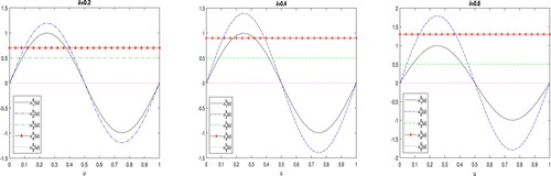The above means that there are five clusters for the coefficients: some are varying with $U_t$ and others are constant. The size of each cluster in this example is the same (i.e. four). Figure 1 plots the five cluster-specific coefficient functions for each value of δ. The larger the value of δ, the further the distance is between these functions, and hence, the easier it is to identify the clusters.

Figure 1. Plots of the cluster-specific coefficient functions. Left panel: $\delta =0.4$; right panel: $\delta =0.8$.

The sample size n is set to be 200, 400 or 600, and the number of replications is N = 500. We first use the kernel method to obtain preliminary nonparametric estimates of the functional coefficients ${\beta }_j^0(\cdot ),j=1,\dots ,p$, with the Epanechnikov kernel $K(z)=\frac{3}{4}(1-z^2{)}_{+}$ and the optimal bandwidth selected from the cross-validation method in Section 4.1. The homogeneity and semi-varying coefficient structure in model (21(21) $Y_t=\sum _{j=1}^p{\beta }_j^0(U_t)X_{tj}+\sigma {\epsilon }_t,t=1,\dots ,n,$(21) ) is ignored in this preliminary estimation. A combination of the kernel-based clustering method in Section 2.1 and the generalised information criterion in Section 2.2 is then used to estimate the homogeneity structure. In order to evaluate the clustering performance, we consider two commonly used measures: Normalised Mutual Information (NMI) and Purity, both of which can be used to examine how close the estimated set of clusters is to the true set of clusters. Letting ${\mathcal{C}}_1=\{{\mathcal{C}}_1^1,\dots ,{\mathcal{C}}_{K_1}^1\}$ and ${\mathcal{C}}_2=\{{\mathcal{C}}_1^2,\dots ,{\mathcal{C}}_{K_2}^2\}$ be two sets of disjoint clusters of $(1,2,\dots ,p)$, the NMI between ${\mathcal{C}}_1$ and ${\mathcal{C}}_2$ is defined as $\mathsf{\text{NMI}}({\mathcal{C}}_1,{\mathcal{C}}_2)=\frac{I({\mathcal{C}}_1,{\mathcal{C}}_2)}{[H({\mathcal{C}}_1)+H({\mathcal{C}}_2)]/2},$ where $H({\mathcal{C}}_1)$ and $H({\mathcal{C}}_2)$ are the entropies of ${\mathcal{C}}_1$ and ${\mathcal{C}}_2$, respectively, and $I({\mathcal{C}}_1,{\mathcal{C}}_2)$ is the mutual information between ${\mathcal{C}}_1$ and ${\mathcal{C}}_2$ defined as $I({\mathcal{C}}_1,{\mathcal{C}}_2)=\sum _{k=1}^{K_1}\sum _{j=1}^{K_2}\left(\frac{|{\mathcal{C}}_k^1\cap {\mathcal{C}}_j^2|}{p}\right){\log }_2\left(\frac{p|{\mathcal{C}}_k^1\cap {\mathcal{C}}_j^2|}{|{\mathcal{C}}_k^1||{\mathcal{C}}_j^2|}\right).$ The NMI measure takes a value between 0 and 1 with a larger value indicating that the two sets of clusters are closer. The Purity measure is defined by (22) $\mathsf{\text{Purity}}({\mathcal{C}}_1,{\mathcal{C}}_2)=\frac{1}{p}\sum _{k=1}^{K_1}\underset{1\le j\le K_2}{max}|{\mathcal{C}}_k^1\cap {\mathcal{C}}_j^2|.$(22) It is easy to find that the Purity measure also takes values between 0 and 1, and if ${\mathcal{C}}_1$ and ${\mathcal{C}}_2$ are equal, then $\mathsf{\text{Purity}}({\mathcal{C}}_1,{\mathcal{C}}_2)=1$. However, the purity measure does not trade off the quality of clustering against the number of clusters. For example, a purity value of 1 is achieved if one set contains singleton clusters. The NMI, by contrast, allows for this trade-off.

We finally identify the clusters with zero coefficients and non-zero constant coefficients using the penalised method introduced in Section 2.3. The tuning parameters in the penalty terms are chosen by the GIC detailed in Section 4.1. In order to measure the accuracy of estimates of the coefficients ${\beta }_j^0(\cdot )$, $1\le j\le p$, we compute the Mean Absolute Estimation Error (MAEE), which, for the preliminary (pre-clustering) kernel estimates, ${\tilde{\beta }}_j(\cdot )$, $1\le j\le p$, is defined as $\mathsf{\text{MAEE (PreC-Kernel)}}=\frac{1}{np}\sum _{t=1}^n\sum _{j=1}^p|{\tilde{\beta }}_j(U_t)-{\beta }_j^0(U_t)|,$ and for the post-clustering kernel estimates, $\mathsf{\text{MAEE (PostC-Kernel)}}=\frac{1}{np}\sum _{t=1}^n\sum _{j=1}^p|{\tilde{\beta }}_j^{\ast }(U_t)-{\beta }_j^0(U_t)|,$ where ${\tilde{\beta }}_j^{\ast }(\cdot )={\tilde{\alpha }}_k(\cdot )$ if $j\in {\tilde{\mathcal{C}}}_{k|\tilde{K}}$, $1\le k\le \tilde{K}$, and ${\tilde{\alpha }}_k(\cdot )={\tilde{\alpha }}_{k|\tilde{K}}(\cdot )$, $1\le k\le \tilde{K}$, are the post-clustering kernel estimates of cluster-specific functional coefficients defined in (6(6) $\begin{array}{rl}{\tilde{\mathit{\alpha }}}_K(u_0)& ={[{\tilde{\alpha }}_{1|k}(u_0),\dots ,{\tilde{\alpha }}_{K|K}(u_0)]}^{{}^{⊺}}\\ & ={[\sum _{t=1}^n{\tilde{\mathbf{X}}}_{t,K}{\tilde{\mathbf{X}}}_{t,K}^{{}^{⊺}}{K}_h(U_t,u_0)]}^{-1}\\ & [\sum _{t=1}^n{\tilde{\mathbf{X}}}_{t,K}{Y}_t{K}_h(U_t,u_0)],\end{array}$(6) ). Let ${\hat{\beta }}_j(\cdot )={\hat{\alpha }}_k(\cdot )$ if $j\in {\tilde{\mathcal{C}}}_{k|\tilde{K}}$, $1\le k\le \tilde{K}$, where ${\hat{\alpha }}_k(\cdot )$, $1\le k\le \tilde{K}$, are the penalised estimates of the cluster-specific functional coefficients obtained by minimising (9(9) ${\mathcal{Q}}_n(\mathit{A},\mathit{B})={\mathcal{L}}_n(\mathit{A},\mathit{B})+{\mathcal{P}}_{n1}(\mathit{A})+{\mathcal{P}}_{n2}(\mathit{B}),$(9) ). The MAEE of the penalised estimates is defined as $\mathsf{\text{MAEE (Penalised)}}=\frac{1}{np}\sum _{t=1}^n\sum _{j=1}^p|{\hat{\beta }}_j(U_t)-{\beta }_j^0(U_t)|.$ The main purpose for considering the MAEE of the post-clustering kernel and penalised estimates for ${\beta }_j^0(\cdot )$, $1\le j\le p$, rather than for ${\alpha }_k^0(\cdot )$, $1\le k\le K_0$, is to avoid having to order the estimated clusters and match each of them to one of the true clusters (as there is no natural way to do this).

Tables 1–3 give the simulation results for the case where the dimension of ${\mathbf{X}}_t$ is 20. Table 1 presents the frequency (over 500 replications) at which a number between 1 and 10 is selected as the number of clusters by the information criterion detailed in Section 2.2. Table 2 gives the average values and standard deviations (in parentheses) of the NMI and Purity measurements over 500 replications. Table 3 reports the average MAEEs and standard deviations (in parentheses) over 500 replications for the pre-clustering kernel estimation, post-clustering kernel estimation and the semiparametric penalised estimation. From Table 1, we can see that when $\delta =0.4$ and the covariates are uncorrelated, the number of clusters can be correctly estimated in about 80% of the replications even when n = 200, and when δ increases to 0.8, this percentage increases to almost 98%. As the sample size increases to 400, the information criterion selects the correct number of clusters in almost all replications. When the correlation coefficient between the covariates is 0.25, the number of clusters is correctly estimated in only 34% of replications when n = 200 and $\delta =0.4$ and in over 70% of replications when $\delta =0.8$. As the sample size increases to 400, this percentage rises to over 98%. However, when $\delta =0.2$, the distances between different coefficient functions become smaller and the number of clusters is often underestimated as 3 or 4, even when the covariates are uncorrelated. When the covariates are correlated, this underestimation becomes worse. In all of the specifications, the estimated number of clusters rarely goes below 3 or above 7. Table 2 shows that when there is no correlation among the covariates and the different coefficient functions are moderately distanced (i.e. $\delta =0.4$ or 0.8), the NMI and Purity values are close to 1 even when the sample size is as small as 200. The increase of the covariates correlation coefficients to 0.25 or the decrease of δ to 0.2 causes the clustering to become less accurate. Finally, the results in Table 3 show that, after identifying the homogeneity and semi-varying coefficient structure, the average MAEE values of the semiparametric penalised estimation are smaller than those of the post-clustering kernel estimation, which in turn are much smaller than those of the pre-clustering kernel estimation. In addition, all three estimation methods improve (with decreasing average MAEE values) as the sample size increases, and their performance becomes slightly worse when the correlation between the covariates increases to 0.25.

Table 1. Results on estimation of cluster number for Example 5.1 with p = 20.

δ	ϱ	n	$\mathsf{\text{K}}=1$	$\mathsf{\text{K}}=2$	$\mathsf{\text{K}}=3$	$\mathsf{\text{K}}=4$	$\mathsf{\text{K}}=5$	$\mathsf{\text{K}}=6$	$\mathsf{\text{K}}=7$	$\mathsf{\text{K}}=8$	$\mathsf{\text{K}}=9$	$\mathsf{\text{K}}=10$
0.2	0	200	0	0	222	185	90	2	1	0	0	0
		400	0	0	2	113	381	4	0	0	0	0
		600	0	0	0	12	488	0	0	0	0	0
0.2	0.25	200	0	1	428	56	8	7	0	0	0	0
		400	0	0	195	223	82	0	0	0	0	0
		600	0	0	22	185	292	1	0	0	0	0
0.4	0	200	0	0	3	54	400	39	4	0	0	0
		400	0	0	0	0	500	0	0	0	0	0
		600	0	0	0	0	500	0	0	0	0	0
0.4	0.25	200	0	0	146	157	170	25	2	0	0	0
		400	0	0	0	3	494	3	0	0	0	0
		600	0	0	0	0	500	0	0	0	0	0
0.8	0	200	0	0	0	1	489	9	1	0	0	0
		400	0	0	0	0	500	0	0	0	0	0
		600	0	0	0	0	500	0	0	0	0	0
0.8	0.25	200	0	0	15	62	365	45	12	1	0	0
		400	0	0	0	0	500	0	0	0	0	0
		600	0	0	0	0	500	0	0	0	0	0

Table 2. Average NMI and Purity for Example 5.1 with p = 20.

		$\varrho =0$		$\varrho =0.25$
δ	n	NMI	Purity	NMI	Purity
0.2	200	0.8340 (0.0605)	0.9729 (0.0432)	0.7778 (0.0462)	0.9771 (0.0497)
	400	0.9590 (0.0495)	0.9865 (0.0265)	0.8641 (0.0676)	0.9916 (0.0226)
	600	0.9925 (0.0240)	0.9964 (0.0137)	0.9467 (0.0588)	0.9938 (0.0185)
0.4	200	0.9593 (0.0566)	0.9743 (0.0472)	0.8459 (0.0880)	0.9503 (0.0567)
	400	1.0000 (0.0000)	1.0000 (0.0000)	0.9971 (0.0148)	0.9981 (0.0106)
	600	1.0000 (0.0000)	1.0000 (0.0000)	1.0000 (0.0000)	1.0000 (0.0000)
0.8	200	0.9952 (0.0230)	0.9958 (0.0211)	0.9368 (0.0774)	0.9596 (0.0583)
	400	1.0000 (0.0000)	1.0000 (0.0000)	1.0000 (0.0000)	1.0000 (0.0000)
	600	1.0000 (0.0000)	1.0000 (0.0000)	1.0000 (0.0000)	1.0000 (0.0000)

Table 3. Average MAEE for Example 5.1 with p = 20.

δ	ϱ	n	PreC-Kernel	PostC-Kernel	Penalised
0.2	0	200	0.1533 (0.0137)	0.0996 (0.0154)	0.0670 (0.0174)
		400	0.0927 (0.0056)	0.0517 (0.0087)	0.0301 (0.0088)
		600	0.0711 (0.0036)	0.0375 (0.0044)	0.0214 (0.0057)
0.2	0.25	200	0.2376 (0.0245)	0.1173 (0.0245)	0.0816 (0.0233)
		400	0.1332 (0.0077)	0.0725 (0.0114)	0.0471 (0.0173)
		600	0.1009 (0.0052)	0.0520 (0.0092)	0.0268 (0.0116)
0.4	0	200	0.1661 (0.0140)	0.0777 (0.0187)	0.0539 (0.0201)
		400	0.0967 (0.0056)	0.0447 (0.0035)	0.0260 (0.0058)
		600	0.0753 (0.0040)	0.0365 (0.0029)	0.0225 (0.0056)
0.4	0.25	200	0.2605 (0.0442)	0.1357 (0.0333)	0.1028 (0.0424)
		400	0.1441 (0.0097)	0.0560 (0.0060)	0.0253(0.0064)
		600	0.1090 (0.0055)	0.0445 (0.0034)	0.0200 (0.0042)
0.8	0	200	0.1918 (0.0161)	0.0778 (0.0132)	0.0460 (0.0132)
		400	0.1083 (0.0062)	0.0488 (0.0041)	0.0253 (0.0048)
		600	0.0832 (0.0043)	0.0393 (0.0029)	0.0223 (0.0037)
0.8	0.25	200	0.3020 (0.0522)	0.1336 (0.0439)	0.0845 (0.0541)
		400	0.1637 (0.0105)	0.0611 (0.0050)	0.0267 (0.0055)
		600	0.1206 (0.0054)	0.0492 (0.0037)	0.0233 (0.0048)

Tables 4–6 give the results for p = 60. Comparing these results with those for p = 20, we can see that as the dimension of the covariates increases, the estimation becomes poorer. However, the overall pattern as δ, or ϱ, or n changes is similar: as δ increases, the estimation becomes more accurate due to the clusters becoming further distanced from each other; as ϱ increases, the results become poorer; and as n increases, the results improve.

Table 4. Results on estimation of cluster number for Example 5.1 with p = 60.

δ	ϱ	n	$\mathsf{\text{K}}=1$	$\mathsf{\text{K}}=2$	$\mathsf{\text{K}}=3$	$\mathsf{\text{K}}=4$	$\mathsf{\text{K}}=5$	$\mathsf{\text{K}}=6$	$\mathsf{\text{K}}=7$	$\mathsf{\text{K}}=8$	$\mathsf{\text{K}}=9$	$\mathsf{\text{K}}=10$
0.2	0	200	25	45	109	115	91	51	31	21	11	1
		400	0	0	287	120	53	24	6	7	2	1
		600	0	0	10	72	347	60	8	2	0	1
0.2	0.25	200	24	190	151	81	34	15	3	2	0	0
		400	8	133	171	74	56	32	17	8	1	0
		600	0	1	439	40	18	2	0	0	0	0
0.4	0	200	22	37	96	87	99	85	37	21	8	8
		400	0	0	4	95	241	76	44	22	14	4
		600	0	0	0	0	488	9	3	0	0	0
0.4	0.25	200	29	148	150	105	41	13	12	2	0	0
		400	4	73	187	106	66	39	18	5	1	1
		600	0	0	225	136	98	29	9	2	1	0
0.8	0	200	11	32	72	112	107	80	36	24	16	10
		400	0	0	0	6	306	83	46	31	17	11
		600	0	0	0	0	500	0	0	0	0	0
0.8	0.25	200	22	74	192	114	64	24	8	2	0	0
		400	0	18	184	116	88	58	20	10	5	1
		600	0	0	25	87	238	107	32	5	6	0

Table 5. Average NMI and Purity for Example 5.1 with p = 60.

		$\varrho =0$		$\varrho =0.25$
δ	n	NMI	Purity	NMI	Purity
0.2	200	0.3115 (0.1723)	0.6422 (0.1820)	0.3134 (0.1234)	0.7607 (0.1363)
	400	0.7660 (0.0509)	0.9370 (0.0932)	0.3913 (0.1415)	0.7507 (0.1413)
	600	0.8888 (0.0541)	0.9336 (0.0525)	0.7484 (0.0485)	0.9668 (0.0488)
0.4	200	0.3029 (0.1496)	0.6088 (0.1717)	0.3190 (0.1285)	0.7498 (0.1349)
	400	0.8296 (0.0932)	0.8758 (0.1057)	0.4128 (0.1281)	0.7288 (0.1265)
	600	0.9934 (0.0182)	0.9949 (0.0191)	0.7582 (0.0605)	0.9197 (0.0657)
0.8	200	0.3232 (0.1248)	0.5980 (0.1531)	0.3577 (0.1276)	0.7345 (0.1208)
	400	0.9034 (0.0943)	0.9082 (0.1061)	0.4658 (0.1107)	0.7188 (0.1196)
	600	0.9999 (0.0016)	1.0000 (0.0007)	0.8508 (0.0808)	0.9085 (0.0708)

Table 6. Average MAEE for Example 5.1 with p = 60.

δ	ϱ	n	PreC-Kernel	PostC-Kernel	Penalised
0.2	0	200	0.3354 (0.0256)	0.3273 (0.0966)	0.3109 (0.0947)
		400	0.1968 (0.0115)	0.1177 (0.0229)	0.0911 (0.0233)
		600	0.1345 (0.0066)	0.0592 (0.0114)	0.0343 (0.0111)
0.2	0.25	200	0.6161 (0.0756)	0.2965 (0.0532)	0.2779 (0.0546)
		400	0.4874 (0.0365)	0.2828 (0.0644)	0.2444 (0.0667)
		600	0.3382 (0.0185)	0.1084 (0.0201)	0.0822 (0.0202)
0.4	0	200	0.3705 (0.0272)	0.3926 (0.0859)	0.3746 (0.0833)
		400	0.2152 (0.0134)	0.1255 (0.0383)	0.0899 (0.0401)
		600	0.1459 (0.0073)	0.0549 (0.0091)	0.0268 (0.0066)
0.4	0.25	200	0.6796 (0.0851)	0.3513 (0.0588)	0.3299 (0.0588)
		400	0.5322 (0.0369)	0.3259 (0.0613)	0.2837(0.0623)
		600	0.3686 (0.0199)	0.1563 (0.0283)	0.1238 (0.0377)
0.8	0	200	0.4365 (0.0375)	0.4897 (0.0836)	0.4687 (0.0814)
		400	0.2546 (0.0149)	0.1390 (0.0442)	0.0960 (0.0469)
		600	0.1713 (0.0084)	0.0627 (0.0084)	0.02998 (0.0059)
0.8	0.25	200	0.8062 (0.0959)	0.4451 (0.0683)	0.4207 (0.0710)
		400	0.6213 (0.0425)	0.3968 (0.0705)	0.3448 (0.0698)
		600	0.4292 (0.0220)	0.1632 (0.0459)	0.1099 (0.0551)

Example 5.2

We consider model (21(21) $Y_t=\sum _{j=1}^p{\beta }_j^0(U_t)X_{tj}+\sigma {\epsilon }_t,t=1,\dots ,n,$(21) ) with p = 20 but with the following homogeneity structure instead: $\begin{array}{rl}& {\beta }_1^0(\cdot )={\alpha }_1^0(\cdot ),{\beta }_2^0(\cdot )={\beta }_3^0(\cdot )={\alpha }_2^0(\cdot ),{\beta }_4^0(\cdot )=\cdots ={\beta }_7^0(\cdot )\equiv {\alpha }_3^0,\\ & {\beta }_8^0(\cdot )=\cdots ={\beta }_{13}^0(\cdot )\equiv {\alpha }_4^0,{\beta }_{14}^0(\cdot )=\cdots ={\beta }_{20}^0(\cdot )\equiv {\alpha }_5^0.\end{array}$ The data generating processes for the random covariates ${\mathbf{X}}_t$, the index variable $U_t$ and the error term ${\epsilon }_t$ are the same as those in Example 5.1. The definitions of ${\alpha }_i^0(\cdot )$ and ${\alpha }_i^0$ are also the same as those in the previous example. However, the sizes of the clusters are now unequal, which are 1, 2, 4, 6, 7, respectively. To save space, we don't provide results for p = 60 for this example.

Tables 7 and 8 report the results for the estimation of the homogeneity structure and Table 9 reports the average MAEEs and standard deviations (in parentheses) for the pre-clustering kernel estimation, the post-clustering kernel estimation and the penalised estimation over 500 replications. Comparing the results in Table 7 with those in Table 1, we find that when $\delta =0.2$, the number of clusters are more likely to be underestimated in Example 5.2 where cluster sizes are unequal. However, as δ increases, the results for the two examples become more and more comparable. The NMI and purity values in Table 8 are similar to those in Table 2, while the MAEE values in Table 9 are smaller than those in Table 3. The latter is mainly due to the fact that more coefficient functions (i.e. 17 out of 20) are constant in Example 5.2.

Table 7. Results on estimation of cluster number for Example 5.2 with p = 20.

δ	ϱ	n	$\mathsf{\text{K}}=1$	$\mathsf{\text{K}}=2$	$\mathsf{\text{K}}=3$	$\mathsf{\text{K}}=4$	$\mathsf{\text{K}}=5$	$\mathsf{\text{K}}=6$	$\mathsf{\text{K}}=7$	$\mathsf{\text{K}}=8$	$\mathsf{\text{K}}=9$	$\mathsf{\text{K}}=10$
0.2	0	200	0	0	76	374	40	9	1	0	0	0
		400	0	0	0	419	81	0	0	0	0	0
		600	0	0	0	363	137	0	0	0	0	0
0.2	0.25	200	0	0	187	281	27	4	1	0	0	0
		400	0	0	8	460	31	0	1	0	0	0
		600	0	0	0	471	29	0	0	0	0	0
0.4	0	200	0	0	0	193	274	30	2	1	0	0
		400	0	0	0	4	495	1	0	0	0	0
		600	0	0	0	0	500	0	0	0	0	0
0.4	0.25	200	0	0	0	306	177	16	1	0	0	0
		400	0	0	0	43	457	0	0	0	0	0
		600	0	0	0	3	497	0	0	0	0	0
0.8	0	200	0	0	0	2	485	11	2	0	0	0
		400	0	0	0	0	499	1	0	0	0	0
		600	0	0	0	0	500	0	0	0	0	0
0.8	0.25	200	0	0	0	16	455	29	0	0	0	0
		400	0	0	0	0	500	0	0	0	0	0
		600	0	0	0	0	500	0	0	0	0	0

Table 8. Average NMI and Purity for Example 5.2 with p = 20.

		$\varrho =0$		$\varrho =0.25$
δ	n	NMI	Purity	NMI	Purity
0.2	200	0.8946 (0.0667)	0.9646 (0.0501)	0.8626 (0.0630)	0.9656 (0.0524)
	400	0.9643 (0.0277)	0.9956 (0.0185)	0.9499 (0.0410)	0.9905 (0.0248)
	600	0.9746 (0.0163)	0.9998 (0.0032)	0.9654 (0.0158)	0.9989 (0.0073)
0.4	200	0.9785 (0.0308)	0.9901 (0.0365)	0.9630 (0.0420)	0.9869 (0.0379)
	400	0.9997 (0.0033)	0.9999 (0.0022)	0.9970 (0.0097)	1.0000 (0.0000)
	600	1.0000 (0.0000)	1.0000 (0.0000)	0.9998 (0.0027)	1.0000 (0.0000)
0.8	200	0.9979 (0.0120)	0.9973 (0.0178)	0.9900 (0.0302)	0.9918 (0.0280)
	400	0.9999 (0.0031)	0.9998 (0.0045)	1.0000 (0.0000)	1.0000 (0.0000)
	600	1.0000 (0.0000)	1.0000 (0.0000)	1.0000 (0.0000)	1.0000 (0.0000)

Table 9. Average MAEE for Example 5.2 with p = 20.

δ	ϱ	n	PreC-Kernel	PostC-Kernel	Penalised
0.2	0	200	0.1092 (0.0092)	0.0634 (0.0142)	0.0415 (0.0168)
		400	0.0714 (0.0049)	0.0369 (0.0050)	0.0213 (0.0061)
		600	0.0571 (0.0035)	0.0303 (0.0032)	0.0169 (0.0042)
0.2	0.25	200	0.1347 (0.0126)	0.0723 (0.0146)	0.0503 (0.0190)
		400	0.0862 (0.0058)	0.0399 (0.0076)	0.0211 (0.0087)
		600	0.0687 (0.0043)	0.0320 (0.0036)	0.0161 (0.0034)
0.4	0	200	0.1179 (0.0100)	0.0534 (0.0102)	0.0410 (0.0100)
		400	0.0755 (0.0049)	0.0358 (0.0042)	0.0167 (0.0040)
		600	0.0597 (0.0033)	0.0287 (0.0030)	0.0134 (0.0031)
0.4	0.25	200	0.1457 (0.0137)	0.0660 (0.0152)	0.0353 (0.0144)
		400	0.0919 (0.0059)	0.0383 (0.0051)	0.0173 (0.0054)
		600	0.0724 (0.0040)	0.0309 (0.0033)	0.0131 (0.0031)
0.8	0	200	0.1343 (0.0113)	0.0622 (0.0096)	0.0304 (0.0080)
		400	0.0843 (0.0050)	0.0394 (0.0042)	0.0188 (0.0042)
		600	0.0664 (0.0036)	0.0315 (0.0033)	0.0157 (0.0037)
0.8	0.25	200	0.1686 (0.0153)	0.0701 (0.0160)	0.0346 (0.0157)
		400	0.1030 (0.0066)	0.0414 (0.0046)	0.0203 (0.0093)
		600	0.0803 (0.0044)	0.0332 (0.0033)	0.0151 (0.0065)

6. Empirical applications

In this section, we apply the developed model and methodology to two real data sets: the Boston house price data and the plasma beta-carotene level data. These two data sets have been extensively analysed in existing studies where functional-coefficient models are usually recommended. However, it is not clear whether certain homogeneity structure among the functional coefficients exists. This motivates us to further examine the modelling structure for these two data sets via the kernel-based clustering method and penalised approach introduced in Section 2.

Example 6.1

We first apply the developed model and methodology to the well-known Boston house price data. This data set has been previously analysed in many studies (cf. Fan and Huang 2005; Cai and Xu 2008; Wang and Xia 2009; Leng 2010). To investigate what factors influencing the house prices, we choose MEDV (the median value of owner-occupied homes in US$1000) as the response variable and the following 13 variables as the explanatory variables: INT (the intercept), CHAS (Charles River dummy variable; $=1$ if tract bounds river, 0 otherwise), RAD (index of accessibility to radial highways), CRIM (crime rate per capita by town), ZN (proportion of residential land zoned for lots over 25,000 sq. ft.), INDUS (proportion of non-retail business acres per town), NOX (nitric oxides concentration in parts per 10 million), RM (average number of rooms per dwelling), AGE (proportion of owner-occupied units built prior to 1940), DIS (weighted distances to five Boston employment centres), TAX (full-value property-tax rate per US$ 10,000), PTRATIO (pupil–teacher ratio by town), and B (1000(Bk−0.63)${}^2,$ where Bk is the proportion of blacks by town). The variable LSTAT (percentage of lower status population) is chosen as the index variable in the varying-coefficient model, which enables us to investigate the interaction of LSTAT with the explanatory variables. The sample size is n = 506. The response variable and all explanatory variables (except the intercept, INT) undergo the Z-score transformation before being fitted: i.e. for any variable, $x_t$, to be transformed, its Z-score is (23) $z_t=\frac{x_t-\overline{x}}{s(x)},t=1,\dots ,506,$(23) where $\overline{x}$ and $s(x)$ are the sample mean and sample standard deviation of $x_t$. Furthermore, as shown in the left panel of Figure 2, the index variable, LSTAT, exhibits strong skewness. Hence, we first take the square-root transformation of this variable to alleviate skewness and then the min–max normalisation: (24) $U_t^{\star }=\frac{U_t-min(U)}{max(U)-min(U)},$(24) where $min(U)$ and $max(U)$ denote the minimum and maximum of the observations of U, respectively. 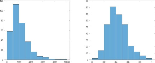After the min–max normalisation, the support of $U_t^{\star }$ becomes $[0,1]$, consistent with the assumption made on the index variable in the asymptotic theory. A histogram of this transformed variable is shown in the right panel of Figure 2.

Figure 2. Histograms for the original and transformed index variable in Example 6.1. Left panel: original data for LSTAT; right panel: LSTAT after the square-root and min-max transformations.

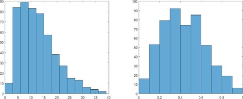
Figure 3 plots the pre-clustering kernel estimated functional coefficients with the optimal bandwidth selected via the leave-one-out cross-validation method. The kernel-based clustering method and the generalised information criterion identify six clusters. The membership of these clusters and the characteristics of their functional coefficients are summarised in Table 10. DIS and TAX are found, by the penalised method, to have constant and similar negative effects on the response, while the variables CHAS, ZN, and B are found to be insignificant. All the other explanatory variables have varying effects on the response as the value of LSTAT changes. Plots of the post-clustering kernel estimates of the functional coefficients and their penalised local linear estimates are shown in Figures 4 and 5, where for each $k=1,\dots ,6$, ${\alpha }_k(\cdot )$ denotes the functional coefficient corresponding to the kth cluster listed in Table 10. The optimal tuning parameters in the penalised method are chosen, by the GIC, as ${\lambda }_1=10$ and ${\lambda }_2=2.3$.

Figure 3. Pre-clustering estimates of the functional coefficients in Example 6.1.

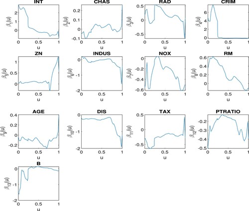
Figure 4. Post-clustering estimates of the functional coefficients in Example 6.1 with ${\alpha }_k(\cdot )$, for each $k=1,2,\dots ,6$, being the estimated functional coefficient corresponding to the kth cluster listed in Table 10.

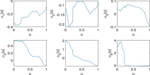
Figure 5. Penalised estimates of the functional coefficients in Example 6.1 with ${\alpha }_k(\cdot )$, for each $k=1,2,\dots ,6$, being the estimated functional coefficient corresponding to the kth cluster listed in Table 10.

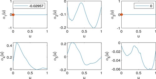
Table 10. The estimated homogeneity structure in Example 6.1.

Clusters	Variables	Coefficient functions
Cluster 1	DIS, TAX	Constant, value is −0.0296
Cluster 2	INDUS, NOX, AGE, PTRATIO	Non-constant, values are negative
Cluster 3	CHAS, ZN, B	Constant, value is 0
Cluster 4	RAD, RM	Non-constant, values are mostly positive
Cluster 5	INT	Non-constant
Cluster 6	CRIM	Non-constant, values are negative

We next compare the out-of-sample predictive performance between the pre-clustering (preliminary) kernel method, the post-clustering kernel method and the proposed penalised method. We randomly split the full sample into a training set of size 400 and a testing set of size 106 and repeat 200 times to reduce randomness in the results obtained. When calculating out-of-sample predictions for the post-clustering and penalised methods, we use the homogeneity structure (i.e. the clusters and their membership) estimated from the full sample but estimate the values of the functional coefficients (evaluated at the LSTAT values belonging to the testing set) or the constant coefficients from the training sets. The predictive performance is measured by Mean Absolute Prediction Error (MAPE), which is defined by (25) $\mathsf{\text{MAPE}}=\frac{1}{n_{\star }}\sum _{t=1}^{n_{\star }}|Y_t^{\star }-{\hat{Y}}_t^{\star }|,$(25) where $n_{\star }$ is the size of the testing set (106 in this example), $Y_t^{\star }$ is a true value of the response variable in the testing sample, and ${\hat{Y}}_t^{\star }$ is the predicted value of $Y_t^{\star }$ using the model estimated from the training sample. Table 11 reports the average MAPE values over 200 replications of random sample splitting. We consider bandwidth values in the range $[0.06,0.18]$ (with equal increment 0.02), which covers the optimal bandwidth of 0.168 for the preliminary kernel estimation and post-clustering kernel estimation. From Table 11, we can see that predicted values calculated from the model estimated by the penalised method have the smallest MAPEs over the range of bandwidth considered. Predictions made from the model estimated by the post-clustering kernel method have slightly larger MAPE values, while predictions from the pre-clustering kernel method have the largest MAPE values. This comparison result shows that the simplified functional-coefficient models from the developed kernel-based clustering and penalised methods provide a more accurate out-of-sample prediction.

Table 11. Average MAPE over 200 times of random sample splitting in Example 6.1.

Method	h = 0.06	h = 0.08	h = 0.10	h = 0.12	h = 0.14	h = 0.16	h = 0.18
PreC-Kernel	0.4957	0.4117	0.3622	0.3254	0.3029	0.2957	0.2944
PostC-Kernel	0.3436	0.3319	0.3091	0.2995	0.2946	0.2919	0.2919
Penalised	0.3273	0.3092	0.2987	0.2913	0.2858	0.2834	0.2844

Example 6.2

In this example, we use the proposed methods to analyse the plasma beta-carotene level data, which have been previously studied by Nierenberg, Stukel, Baron, Dain, and Greenberg (1989), Wang and Li (2009) and Kai et al. (2011). The data were collected from 315 patients and are downloadable from the StatLib database http://lib.stat.cmu.edu/datasets/Plasma_Retinol. The primary interest is to investigate the relationship between personal characteristics and dietary factors, and plasma concentrations of beta-carotene. The response variable is chosen as BETAPLASMA (plasma beta-carotene level, ng/ml) and the candidate explanatory variables include INT (the intercept), AGE (years), QUETELET (Quetelet index, weight/height${}^2$), CALORIES (number of calories consumed per day), FAT (grams of fat consumed per day), FIBRE (grams of fibre consumed per day), ALCOHOL (number of alcoholic drinks consumed per week), CHOLESTEROL (cholesterol consumed per day). The data set also contains categorical variables: SEX (1 = male, 2 = female), SMOKSTAT (smoking status, 1 = never, 2 = former, 3 = current smoker), VITUSE (vitamin use, 1 = yes, fairly often, 2 = yes, not often, 3 = no). We convert these into dummy variables: FEMALE ( = 1 if SEX = 2, 0 otherwise), NONSMOKER ( = 1 if SMOKSTAT = 1, 0 otherwise), FORMERSMOKER (= 1 if SMOKSTAT = 2, 0 otherwise), FREQVITUSE ( = 1 if VITUSE = 1, 0 otherwise), OCCAVITUSE ( = 1 if VITUSE = 2, 0 otherwise), and also include them as explanatory variables. As in Kai et al. (2011), the index variable is chosen as BETADIET (dietary beta-carotene consumed, mcg per day). We again transform the response and explanatory variables (except the intercept, INT) by the Z-score method defined in (23(23) $z_t=\frac{x_t-\overline{x}}{s(x)},t=1,\dots ,506,$(23) ). As can be seen from the left panel of Figure 6, the index variable BETADIET also exhibits high skewness, so we first transform it by the square-root operator and then the min–max operator in (24(24) $U_t^{\star }=\frac{U_t-min(U)}{max(U)-min(U)},$(24) ). Histograms for the original data for BETADIET as well as the transformed data are given in Figure 6.

Figure 6. Histograms for the original and transformed index variable in Example 6.2. Left panel: original data for BETADIET, right panel: BETADIET after the square-root and min-max transformations.

We again consider using a functional-coefficient model. In the preliminary kernel estimation, the Epanechnikov kernel $K(z)=\frac{3}{4}(1-z^2{)}_{+}$ is used and the optimal bandwidth is determined via the cross-validation method in Section 4.1. We combine the kernel-based clustering method and penalised local linear estimation (with the tuning parameters ${\lambda }_1=6.5$ and ${\lambda }_2=3$ chosen by the GIC method) to explore the homogeneity structure among the functional coefficients. Three distinct clusters are identified. The membership of each cluster and the characteristic of the corresponding coefficient function are summarised in Table 12. The pre-clustering estimates of all functional coefficients and the post-clustering and penalised estimates of the cluster-specific functional coefficients are plotted in Figures 7–9.

Figure 7. Pre-clustering estimates of the functional coefficients in Example 6.2.

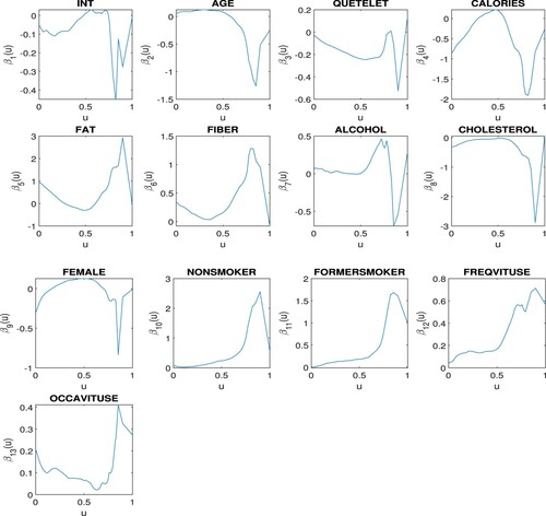
Figure 8. Post-clustering estimates of the functional coefficients in Example 6.2 with ${\alpha }_k(\cdot )$, for each k = 1, 2, 3, being the estimated functional coefficient corresponding to the kth cluster listed in Table 12.

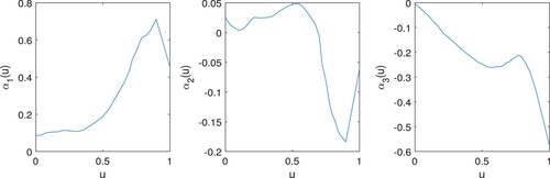
Figure 9. Penalised estimates of the functional coefficients in Example 6.2 with ${\alpha }_k(\cdot )$, for each k = 1, 2, 3, being the estimated functional coefficient corresponding to the kth cluster listed in Table 12.

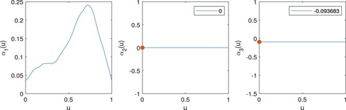
Table 12. The estimated homogeneity structure in Example 6.2.

Clusters	Variables	Coefficient functions
Cluster 1	FIBRE, NONSMOKER,	Non-constant,
	FORMERSMOKER, FREQVITUSE	values are positive
Cluster 2	INT, AGE, CALORIES, ALCOHOL,	Constant,
	CHOLESTEROL, FEMALE, OCCAVITUSE	value is 0
Cluster 3	QUETELET, FAT	Constant, value is −0.0937

The kernel clustering and shrinkage estimation results show that FIBRE, NONSMOKER, FORMERSMOKER, FREQVITUSE form a cluster and their effects on the response variable, the beta-carotene level, are positive, which implies that higher fibre intake, no smoking and frequent vitamin use are helpful for increasing beta-carotene levels. The variables INT (intercept), AGE, CALORIES, ALCOHOL, CHOLESTEROL, FEMALE, and OCCAVITUSE are found to be insignificant, while QUETELET and FAT are found to have negative effects on beta-carotene levels.

As in Example 6.1, we further compare the out-of-sample predictive performance between the preliminary kernel, post-clustering kernel and penalised methods. We randomly divide the full sample (315 observations) into a training set of size 250 and a testing set of size 65, and repeat the random sample splitting 200 times and compute the average MAPE values. The predictions are calculated in the same way as in Example 6.1. The range of bandwidth values considered is between 0.20 and 0.32 with an increment of 0.02. The results are reported in Table 13. From the table, we find that the penalised and post-clustering kernel methods provide more accurate out-of-sample prediction in terms of MAPE defined in (25(25) $\mathsf{\text{MAPE}}=\frac{1}{n_{\star }}\sum _{t=1}^{n_{\star }}|Y_t^{\star }-{\hat{Y}}_t^{\star }|,$(25) ) than the preliminary kernel method, with the penalised method slightly outperforming the post-clustering kernel method when the bandwidth is smaller.

Table 13. Average MAPE over 200 times of random sample splitting in Example 6.2.

Method	h = 0.20	h = 0.22	h = 0.24	h = 0.26	h = 0.28	h = 0.30	h = 0.32
PreC-Kernel	0.6800	0.6761	0.6322	0.6209	0.6115	0.6114	0.6045
PostC-Kernel	0.5895	0.5826	0.5790	0.5754	0.5743	0.5730	0.5712
Penalised	0.5788	0.5768	0.5752	0.5751	0.5750	0.5746	0.5741

7. Conclusion

In this paper, we have developed the kernel-based hierarchical clustering method and a generalised version of information criterion to uncover the latent homogeneity structure in the functional-coefficient models. Furthermore, the penalised local linear estimation approach is used to separate out the zero-constant cluster, the non-zero constant-coefficient clusters and the functional-coefficient clusters. The asymptotic theory in Section 3 shows that the estimation for the true number of clusters and the true set of clusters is consistent in the large-sample case. In the simulation study, we find that the proposed estimation methodology outperforms the direct nonparametric kernel estimation which ignores the latent structure in the model. In the empirical application to the Boston house price data and plasma beta-carotene level data, we show that the nonparametric functional-coefficient model can be substantially simplified with reduced numbers of unknown parametric and nonparametric components. As a result, the out-sample mean absolute prediction errors using the developed approach are significantly smaller than those using the naive kernel method which ignores the latent homogeneity structure among the functional coefficients.

Acknowledgments

The authors thank the Editor-in-Chief, an Associate Editor and two reviewers for their valuable comments, which improve the former version of the paper.

Disclosure statement

No potential conflict of interest was reported by the author(s).

Additional information

Funding

Chen's research was partially supported by Grant 65617357 from the Economic and Social Research Council of the United Kingdom.

References

- Bondell, H.D., and Reich, B.J. (2008), ‘Simultaneous Regression Shrinkage, Variable Selection and Supervised Clustering of Predictors with OSCAR’, Biometrics, 64(1), 115–123.
- Cai, Z., Fan, J., and Yao, Q. (2000), ‘Functional-Coefficient Regression Models for Nonlinear Time Series’, Journal of the American Statistical Association, 95(451), 941–956.
- Cai, Z., and Xu, X. (2008), ‘Nonparametric Quantile Estimations for Dynamic Smooth Coefficient Models’, Journal of the American Statistical Association, 103(484), 1595–1608.
- Chen, J., Li, D., and Xia, Y. (2019), ‘Estimation of a Rank-Reduced Functional-Coefficient Panel Data Model in Presence of Serial Correlation’, Journal of Multivariate Analysis, 173, 456–479.
- Cheng, M., Zhang, W., and Chen, L. (2009), ‘Statistical Estimation in Generalized Multiparameter Likelihood Models’, Journal of the American Statistical Association, 104(487), 1179–1191.
- Everitt, B.S., Landau, S., Leese, M., and Stahl, D. (2011), Cluster Analysis (5th ed.), Wiley Series in Probability and Statistics. Wiley.
- Fan, J., and Gijbels, I. (1996), Local Polynomial Modelling and Its Applications, London: Chapman and Hall.
- Fan, J., and Huang, T. (2005), ‘Profile Likelihood Inferences on Semiparametric Varying-Coefficient Partially Linear Models’, Bernoulli, 11(6), 1031–1057.
- Fan, J., and Li, R. (2001), ‘Variable Selection Via Nonconcave Penalized Likelihood and Its Oracle Properties’, Journal of the American Statistical Association, 96(456), 1348–1360.
- Fan, J., Ma, Y., and Dai, W. (2014), ‘Nonparametric Independence Screening in Sparse Ultra-High Dimensional Varying Coefficient Models’, Journal of the American Statistical Association, 109(507), 1270–1284.
- Fan, Y., and Tang, C.Y. (2013), ‘Tuning Parameter Selection in High Dimensional Penalized Likelihood’, Journal of the Royal Statistical Society, Series B (Statistical Methodology), 75(3), 531–552.
- Fan, J., and Zhang, W. (1999), ‘Statistical Estimation in Varying Coefficient Models’, The Annals of Statistics, 27(5), 1491–1518.
- Fan, J., and Zhang, W. (2008), ‘Statistical Methods with Varying Coefficient Models’, Statistics and Its Interface, 1(1), 179–195.
- Green, P., and Silverman, B. (1994), Nonparametric Regression and Generalized Linear Models: A Roughness Penalty Approach, London: Chapman and Hall/CRC.
- Jiang, Q., Wang, H., Xia, Y., and Jiang, G. (2013), ‘On a Principal Varying Coefficient Model’, Journal of the American Statistical Association, 108(501), 228–236.
- Kai, B., Li, R., and Zou, H. (2011), ‘New Efficient Estimation and Variable Selection Methods for Semiparametric Varying-Coefficient Partially Linear Models’, The Annals of Statistics, 39(1), 305–332.
- Ke, Z., Fan, J., and Wu, Y. (2015), ‘Homogeneity Pursuit’, Journal of the American Statistical Association, 110(509), 175–194.
- Ke, Y., Li, J., and Zhang, W. (2016), ‘Structure Identification in Panel Data Analysis’, The Annals of Statistics, 44(3), 1193–1233.
- Lee, E.R., and Mammen, E. (2016), ‘Local Linear Smoothing for Sparse High Dimensional Varying Coefficient Models’, Electronic Journal of Statistics, 10(1), 855–894.
- Leng, C. (2010), ‘Variable Selection and Coefficient Estimation Via Regularized Rank Regression’, Statistica Sinica, 20, 167–181.
- Li, D., Ke, Y., and Zhang, W. (2015), ‘Model Selection and Structure Specification in Ultra-High Dimensional Generalised Semi-Varying Coefficient Models’, The Annals of Statistics, 43(6), 2676–2705.
- Liu, J., Li, R., and Wu, R. (2014), ‘Feature Selection for Varying Coefficient Models with Ultrahigh Dimensional Covariates’, Journal of the American Statistical Association, 109(505), 266–274.
- Nierenberg, D., Stukel, T., Baron, J., Dain, B., and Greenberg, E. (1989), ‘Determinants of Plasma Levels of Beta-Carotene and Retinol’, American Journal of Epidemiology, 130(3), 511–521.
- Park, B.U., Mammen, E., Lee, Y.K., and Lee, E.R. (2015), ‘Varying Coefficient Regression Models: A Review and New Developments’, International Statistical Review, 83(1), 36–64.
- Rencher, A.C., and Christensen, W.F. (2012), Methods of Multivariate Analysis (3rd ed.), Wiley Series in Probability and Statistics. Wiley.
- Schwarz, G. (1978), ‘Estimating the Dimension of a Model’, The Annals of Statistics, 6(2), 461–464.
- Shen, X., and Huang, H.C. (2010), ‘Group Pursuit Through a Regularization Solution Surface’, Journal of the American Statistical Association, 105(490), 727–739.
- Su, L., Shi, Z., and Phillips, P.C.B. (2016), ‘Identifying Latent Structures in Panel Data’, Econometrica, 84(6), 2215–2264.
- Su, L., Wang, X., and Jin, S. (2019), ‘Sieve Estimation of Time-Varying Panel Data Models with Latent Structures’, Journal of Business and Economic Statistics, 37(2), 334–349.
- Tibshirani, R., Saunders, M., Rosset, S., Zhu, J., and Knight, K. (2005), ‘Sparsity and Smoothness Via the Fused Lasso’, Journal of the Royal Statistical Society, Series B (Statistical Methodology), 67(1), 91–108.
- Vogt, M., and Linton, O. (2017), ‘Classification of Nonparametric Regression Functions in Longitudinal Data Models’, Journal of the Royal Statistical Society, Series B (Statistical Methodology), 79(1), 5–27.
- Wand, M.P., and Jones, M.C. (1995), Kernel Smoothing, London: Chapman and Hall.
- Wang, L., and Li, R. (2009), ‘Weighted Wilcoxon-Type Smoothly Clipped Absolute Deviation Method’, Biometrics, 65(2), 564–571.
- Wang, H., and Xia, Y. (2009), ‘Shrinkage Estimation of the Varying-Coefficient Model’, Journal of the American Statistical Association, 104(486), 747–757.
- Xia, Y., Zhang, W., and Tong, H. (2004), ‘Efficient Estimation for Semivarying-Coefficient Models’, Biometrika, 91(3), 661–681.