A novel framework for joint sparse clustering and alignment of functional data

Abstract

A novel framework for sparse functional clustering that also embeds an alignment step is here proposed. Sparse functional clustering entails estimating the parts of the curves' domains where their grouping structure shows the most. Misalignment is a well-known issue in functional data analysis, that can heavily affect functional clustering results if not properly handled. Therefore, we develop a sparse functional clustering procedure that accounts for the possible curve misalignment: the coherence of the functional measure used in the clustering step to the class where the warping functions are chosen is ensured, and the well-posedness of the sparse clustering problem is proved. A possible implementing algorithm is also proposed, that jointly performs all these tasks: clustering, alignment, and domain selection. The method is tested on simulated data in various realistic situations, and its application to the Berkeley Growth Study data and to the AneuRisk65 dataset is discussed.

KEYWORDS:

• Functional data
• clustering
• sparse methods
• misalignment

AMS:

• 62H30
• 62M99

1. Introduction

Finding sparse solutions to clustering problems has emerged as a hot topic in recent years, both in the statistics and in the machine learning community (see Friedman and Meulman 2004; Witten and Tibshirani 2010; Elhamifar and Vidal 2013, among the many possible references). However, only very recently the problem started to receive attention also in the functional data community, surprisingly enough given the natural link between the two frameworks: functional data analysis (FDA) aims at developing statistical methods for infinite-dimensional data, and sparsity is more likely when data are high-dimensional. There are two main research lines where sparsity has been treated in the FDA literature: (i) as each functional datum is in reality observed on a finite grid, sparsity may occur through a local heterogeneity in the frequency of the discretisation, or in other words the data might be sparsely observed (James, Hastie, and Sugar 2000; Yao, Müller, and Wang 2005; Müller and Yang 2010; Di, Crainiceanu, and Jank 2014; Yao, Wu, and Zou 2016; Stefanucci, Sangalli, and Brutti 2018; Kraus 2019); (ii) more naturally linked to the functional form of the data, sparsity can be defined as local heterogeneity in the concentration of information into the functional space: this aspect has been studied in the regression setting, mainly under linear assumptions (James, Wang, and Zhu 2009; McKeague and Sen 2010; Kneip and Sarda 2011; Aneiros and Vieu 2014; Novo, Aneiros, and Vieu 2019; Bernardi, Canale, and Stefanucci 2023). There has also been some work on sparse functional PCA (Allen 2013; Huang, Shen, and Buja 2009; Di, Crainiceanu, Caffo, and Punjabi 2009; Bauer, Scheipl, Küchenhoff, and Gabriel 2021), and on domain selection in inferential approaches such as functional ANOVA (Pini and Vantini 2016, 2017; Pini, Vantini, Colosimo, and Grasso 2018). However, very few proposals deal with unsupervised learning: when it comes to methods specifically targeted to clustering, some recent approaches (Fraiman, Gimenez, and Svarc 2016; Berrendero, Cuevas, and Pateiro-López 2016a; Berrendero, Cuevas, and Torrecilla 2016b; Floriello and Vitelli 2017; Centofanti, Lepore, and Palumbo 2023) propose to cluster the curves while jointly detecting the most relevant portions of their domain to the clustering purposes. The latent assumption is redundancy of information: curves cluster only on a reduced part of the domain, while most of the observed functional signal might be totally irrelevant to the scopes of the analysis. In this latter framework, a very interesting recent sparse functional clustering proposal is Centofanti et al. (2023), where the model-based SaS-Funclust method is introduced to cluster a set of curves while also selecting cluster-specific portions of the domain where the curves differ the most. However, neither this latter approach nor the less recent ones account for possible misalingment issues in the set of curves.

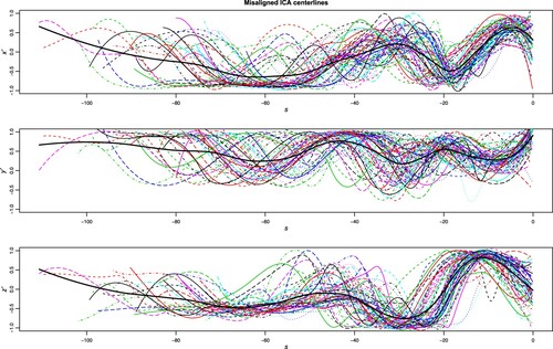
Nonetheless, misalignment represents a frequent issue when dealing with curve clustering: curves might show a phase variability, describing some abscissa variation ancillary to the scopes of the analysis (e.g. biological clock, measurement start, length of the task,…), while the scope of a clustering method is, instead, to capture the amplitude variability. An evident example of this problem is shown in Figure 1, where the curves from the AneuRisk65¹ dataset are displayed: the data consist in the three spatial coordinates (in mm) of 65 Internal Carotid Artery (ICA) centrelines, measured on a fine grid of points along a curvilinear abscissa (in mm), decreasing from the terminal bifurcation of the ICA towards the heart. Estimates of these three-dimensional curves are obtained by means of three-dimensional free-knot regression splines, as described in Sangalli, Secchi, Vantini, and Veneziani (2009b). The first derivatives $x^{\mathrm{\prime }}$, $y^{\mathrm{\prime }}$ and $z^{\mathrm{\prime }}$ (preferred to the ICA original coordinates, which depend on the location of the scanned volume) of the estimated curves are displayed in the figure: the apparent phase variability is strongly dependent on the dimensions and proportions of patients' skulls, and this nuisance variability is meaningless when the study of the heterogeneity of the cerebral morphology is concerned.

Figure 1. Data from the AneuRisk65 dataset. From top to bottom, first derivative of the three spatial coordinates ($x^{\mathrm{\prime }}$, $y^{\mathrm{\prime }}$ and $z^{\mathrm{\prime }}$, respectively) of the ICA centrelines of 65 subjects suspected to be affected by cerebral aneurysm.

As is evident from inspection of Figure 1, misalignment can represent a very substantial proportion of the variability present in the functional dataset, and therefore it might heavily affect and confound the clustering results if not properly handled (Marron, Ramsay, Sangalli, and Srivastava 2015): many authors have studied this problem in recent years (see the nice review by Jacques and Preda (2014)), and claim that jointly decoupling the two sources of variation, thus aligning and clustering the curves jointly, is often convenient (Chiou and Li 2007; Sangalli, Secchi, Vantini, and Vitelli 2010a, 2010b; Zhang and Telesca 2014; Zeng, Qing Shi, and Kim 2019; Fu 2019). When aiming at sparse clustering, and when the curves are also misaligned, a very common approach is to first align the curves and then use a sparse functional clustering method to estimate the groups and select the domain (as we have previously proposed for analysing the Berkeley Growth study data in Floriello and Vitelli 2017). Given the known benefits of joint clustering and alignment (see, e.g. Figure 8 in Sangalli et al. (2010b), and Figure 2 in Mattar, Hanson, and Learned-Miller (2012)), the starting point for this paper is thus to adapt functional sparse clustering to align the data as well. The only available alternative to such purpose is the method very recently proposed in Cremona and Chiaromonte (2023) for the analysis of omics signals, that identifies local amplitude features (the so called ‘motifs’) while accounting for phase variability. However, the latter method is targeted to the idea of discovering the functional motifs (i.e. typical local shapes that might recur within each curve, or across several curves in the sample), while our framework follows the ‘domain selection’ strategy.

In this paper we propose a functional clustering approach that jointly aligns the curves, and that also performs domain selection, meaning that it estimates the portions of the domain where the grouping structure mostly shows. The problem is correctly framed, from a mathematical viewpoint, as a variational problem having the grouping structure, the warping functions, and the domain selector as a solution. Some properties are required to the functional space (and to the associated metric in particular), and to the class where the warping functions are chosen, to ensure the well-posedness of such variational problem. An iterative implementing algorithm, rooted both on the K-means clustering and alignment algorithm introduced in Sangalli et al. (2010b), and on the sparse functional clustering method described in Floriello and Vitelli (2017), is also proposed. The paper is structured as follows: Section 2 gives all the methodological details on the sparse clustering and alignment proposal, while the associated implementing algorithm is described in Section 3. The results of several simulation studies are reported in Section 4, and the application of the proposed methodology to the Berkeley Growth Study data (Tuddenham 1954) and to the AneuRisk 65 dataset (Sangalli, Secchi, Vantini, and Veneziani 2009a) are described in Sections 5 and 6, respectively. Finally, some conclusions and discussion of further developments are given in Section 7.

2. Joint sparse clustering and alignment: a unified framework

In this section we provide the mathematical framework for embedding both the alignment step and the sparsity constraint into the variational problem defining functional clustering in full generality. The clustering and alignment variational problem is first defined in Section 2.1, then the sparsity constraint is described in Section 2.2, and finally the unified variational problem for solving the sparse clustering and alignment problem is proposed in Section 2.3. Some theoretical considerations on consistency and well-posedness in a more general mathematical setting are also discussed in Section 2.4.

2.1. Joint clustering and alignment: decoupling phase and amplitude variability

Let $(D,\mathcal{F},\mu )$ be a measure space, with $D\subset \mathbb{R}$ compact, $\mathcal{F}$ a functional space suited to the application at hand (assume $L^2\left(D\right)$ for the time being), and μ the Lebesgue measure. Let $f_1,\dots ,f_n\in \mathcal{F}$ be a functional dataset, and W the class of warping functions indicating the allowed transformations of the abscissa to align the curves.

A very popular approach in the FDA literature is to study the amplitude and phase variation in a functional dataset via equivalence classes (see Srivastava, Wu, Kurtek, Klassen, and Marron 2011 and Srivastava and Klassen 2016 for a nice introduction): in such approach, clustering can be defined via a proper and mathematically consistent optimisation problem, where alignment is performed by selecting, for each curve in the dataset, an optimal aligning function within a class W. To ensure the well-posedness of the resulting optimisation problem, some properties are required to $\mathcal{F}$ and W (Vantini 2012):

1. $\mathcal{F}$ is a metric space equipped with the metric $d(\cdot ,\cdot ):\mathcal{F}\times \mathcal{F}\to {\mathbb{R}}_0^{+}$ that measures the distance between two curves;

2. W is a sub-group, with respect to composition ○, of the group of continuous automorphisms;

3. $\mathrm{\forall f}\in \mathcal{F},\mathrm{\forall h}\in W$ we have that $f\circ h\in \mathcal{F};$

4. W-invariance property of $d(\cdot ,\cdot )$: for any $f_1,f_2\in \mathcal{F}$ and any $h\in W$ (1) $d(f_1,f_2)=d(f_1\circ h,f_2\circ h),$(1) meaning that it is not possible to create fictitious variations in the distance between two curves $f_1$ and $f_2$ by warping both $f_1$ and $f_2$ with the same warping function h.

While properties (i)–(iii) are quite natural requirements, the W-invariance property (iv) of the metric d as expressed in (1(1) $d(f_1,f_2)=d(f_1\circ h,f_2\circ h),$(1) ) is particularly crucial, since it ensures the well-posedness of the joint clustering (based on the definition of d) and alignment (based on the definition of W) problem. Moreover, it is the W-invariance property that ensures the possibility to compare equivalence classes of functions, and not just individual functions: specifically, the equivalence class of a function $f\in \mathcal{F}$ includes all the versions of the function after its warping via an element of $h\in W$, i.e. $f\circ h.$ Therefore, the properties (i)–(iv) above ensure a coherent framework for decoupling phase and amplitude variability: phase variation is incorporated within equivalence classes, while amplitude variation appears across equivalence classes.

After formulating the problem of decoupling phase and amplitude variability in the functional dataset $f_1,\dots ,f_n\in \mathcal{F}$, it is possible to properly define clustering and alignment as a variational problem: indeed, the most popular clustering methods (such as K-means) are named distance-based, as they entail finding the optimal cluster partition $\{C_1,\dots ,C_K\}$ by solving an optimisation problem based on a measure of the between-cluster distances, depending on the chosen metric d. Given a fixed number K of groups, the clustering and alignment variational problem can be then given as: find the set of optimal warping functions $\{{\tilde{h}}_1,\dots ,{\tilde{h}}_n\}\in W$ and the optimal cluster partition $\{{\tilde{C}}_1,\dots ,{\tilde{C}}_K\}$ maximising (2) $\underset{\{h_1,\dots ,h_n\}\in W,\{C_1,\dots ,C_K\}}{max}{\int }_{D}g\left(f_1\right(h_1\left(x\right)),\dots ,f_n(h_n\left(x\right));\{C_1,\dots ,C_K\left\}\right)\mathrm{d}x,$(2) where we assume $f_i\in L^2\left(D_i\right)$, $D_i$ being the warped domain of each function (compact), and $D=\bigcup _{i=1}^n{D}_i$ being the union of the warped domains of the functions in the dataset. We use dx instead of $\mathrm{d\mu }\left(x\right)$ for ease of notation. The function $g(\cdot )$ defines the point-wise between-cluster sum-of-squares of the functions in the dataset, which depends on d. A quite natural choice for d in this functional space is the normalised $L^2$ norm (3) $d(f_1,f_2)=\frac{1}{\sqrt{\mu (D_1\cap D_2)}}{\left({\int }_{D_1\cap D_2}\right(f_1\left(x\right)-f_2\left(x\right){)}^2\mathrm{d}x)}^{1/2},$(3) since this choice ensures that properties (i)–(iv) above hold when the group of strictly increasing affine transformations is used as the class for warping functions (4) $W=\{h:h(x)=\mathrm{ax}+b\mathrm{with}a\in {\mathbb{R}}^{+},b\in \mathbb{R}\}.$(4) Note that the choice of W in (4(4) $W=\{h:h(x)=\mathrm{ax}+b\mathrm{with}a\in {\mathbb{R}}^{+},b\in \mathbb{R}\}.$(4) ) is a relatively simple one, which however has proved to be effective in practice (Sangalli et al. 2009a, 2010a), as a linear warping is locally a good approximation of any non-linear pattern that phase variability would realistically assume. Moreover, this choice does not require a warping function to be a strictly increasing function with fixed extremes, e.g. such that $h\left(0\right)=0$ and $h\left(1\right)=1$, as is very common in the literature on curve registration (Kneip and Ramsay 2008): this is a mathematically convenient assumption that is however not necessarily realistic in practice. And finally, very few alternative choices of the couple $(d,W)$ verify the properties (i)–(iv), which we deem to be necessary for a coherent mathematical formulation of the clustering and alignment problem; one alternative would be to use the Fisher-Rao metric (Srivastava et al. 2011), which is unfortunately quite difficult to interpret. See Section 7 for some additional comments on the choice of W.

Given the choice in (3(3) $d(f_1,f_2)=\frac{1}{\sqrt{\mu (D_1\cap D_2)}}{\left({\int }_{D_1\cap D_2}\right(f_1\left(x\right)-f_2\left(x\right){)}^2\mathrm{d}x)}^{1/2},$(3) ), the point-wise between-cluster sum-of-squares in (2(2) $\underset{\{h_1,\dots ,h_n\}\in W,\{C_1,\dots ,C_K\}}{max}{\int }_{D}g\left(f_1\right(h_1\left(x\right)),\dots ,f_n(h_n\left(x\right));\{C_1,\dots ,C_K\left\}\right)\mathrm{d}x,$(2) ) takes the form (5) $\begin{array}{rl}& g\left(f_1\right(h_1\left(x\right)),\dots ,f_n(h_n\left(x\right));\{C_1,\dots ,C_K\left\}\right)=\\ & =\frac{1}{n}\sum _{i,j=1}^n\{{\left(f_i\right(h_i\left(x\right))-f_j(h_j\left(x\right)\left)\right)}^2\cdot \frac{1_{\left\{h_i^{-1}\right(D_i)\cap h_j^{-1}(D_j\left)\right\}}\left(x\right)}{\sqrt{\mu \left(h_i^{-1}\right(D_i)\cap h_j^{-1}(D_j\left)\right)}}\}\\ & -\sum _{k=1}^K\frac{1}{n_k}\sum _{i,j\in C_k}\{{\left(f_i\right(h_i\left(x\right))-f_j(h_j\left(x\right)\left)\right)}^2\cdot \frac{1_{\left\{h_i^{-1}\right(D_i)\cap h_j^{-1}(D_j\left)\right\}}\left(x\right)}{\sqrt{\mu \left(h_i^{-1}\right(D_i)\cap h_j^{-1}(D_j\left)\right)}}\},\end{array}$(5) where $n_k=|C_k|$ for all $k=1,\dots ,K.$

Sangalli et al. (2010b) proposed a strategy for tackling the variational problem (2(2) $\underset{\{h_1,\dots ,h_n\}\in W,\{C_1,\dots ,C_K\}}{max}{\int }_{D}g\left(f_1\right(h_1\left(x\right)),\dots ,f_n(h_n\left(x\right));\{C_1,\dots ,C_K\left\}\right)\mathrm{d}x,$(2) ) that is based on an iterative algorithm inspired by the functional K-means. Even if the algorithm set-up was showed in a different setting than that defined by the choices in (3(3) $d(f_1,f_2)=\frac{1}{\sqrt{\mu (D_1\cap D_2)}}{\left({\int }_{D_1\cap D_2}\right(f_1\left(x\right)-f_2\left(x\right){)}^2\mathrm{d}x)}^{1/2},$(3) ) and (4(4) $W=\{h:h(x)=\mathrm{ax}+b\mathrm{with}a\in {\mathbb{R}}^{+},b\in \mathbb{R}\}.$(4) ), the proposal is completely general, so that the same choices have been successfully used in subsequent papers (Abramowicz et al. 2017 among others). The so called K-Means Alignment (KMA) is an iterative algorithm alternating between the following two steps:

1. holding the current cluster partition $\{C_1,\dots ,C_K\}$ fixed, solve the alignment problem alone by maximising criterion (2(2) $\underset{\{h_1,\dots ,h_n\}\in W,\{C_1,\dots ,C_K\}}{max}{\int }_{D}g\left(f_1\right(h_1\left(x\right)),\dots ,f_n(h_n\left(x\right));\{C_1,\dots ,C_K\left\}\right)\mathrm{d}x,$(2) ) to find the current set of optimal warping functions $\{{\tilde{h}}_1,\dots ,{\tilde{h}}_n\}$;

2. holding the current set of warping functions $\{h_1,\dots ,h_n\}$ fixed, find the current optimal cluster partition $\{{\tilde{C}}_1,\dots ,{\tilde{C}}_K\}$ via a functional K-means step applied to the aligned functions.

The algorithm stops when convergence is reached, i.e. when no changes are observed in $\{{\tilde{C}}_1,\dots ,{\tilde{C}}_K\}$ at two subsequent iterations. While Step 2. simply involves functional clustering, Step 1. can be more tricky, as is based on an optimisation problem. However, since the optimal warping functions ${\tilde{h}}_i$ for $i=1,\dots ,n$ are conditionally independent given the cluster templates, the alignment of each curve can be carried out in parallel, thus greatly simplifying the computational implementation. Indeed Step 2. of the KMA algorithm involves not only finding the best partition $\{{\tilde{C}}_1,\dots ,{\tilde{C}}_K\}$, but also then calculating the cluster template associated to each cluster.

Remark

Note that the variational problem defined by (2(2) $\underset{\{h_1,\dots ,h_n\}\in W,\{C_1,\dots ,C_K\}}{max}{\int }_{D}g\left(f_1\right(h_1\left(x\right)),\dots ,f_n(h_n\left(x\right));\{C_1,\dots ,C_K\left\}\right)\mathrm{d}x,$(2) ) and (5(5) $\begin{array}{rl}& g\left(f_1\right(h_1\left(x\right)),\dots ,f_n(h_n\left(x\right));\{C_1,\dots ,C_K\left\}\right)=\\ & =\frac{1}{n}\sum _{i,j=1}^n\{{\left(f_i\right(h_i\left(x\right))-f_j(h_j\left(x\right)\left)\right)}^2\cdot \frac{1_{\left\{h_i^{-1}\right(D_i)\cap h_j^{-1}(D_j\left)\right\}}\left(x\right)}{\sqrt{\mu \left(h_i^{-1}\right(D_i)\cap h_j^{-1}(D_j\left)\right)}}\}\\ & -\sum _{k=1}^K\frac{1}{n_k}\sum _{i,j\in C_k}\{{\left(f_i\right(h_i\left(x\right))-f_j(h_j\left(x\right)\left)\right)}^2\cdot \frac{1_{\left\{h_i^{-1}\right(D_i)\cap h_j^{-1}(D_j\left)\right\}}\left(x\right)}{\sqrt{\mu \left(h_i^{-1}\right(D_i)\cap h_j^{-1}(D_j\left)\right)}}\},\end{array}$(5) ) is completely general, and can be adapted to the choices of $\mathcal{F},$ W and d most suited to the problem at hand, as detailed in Section 2.4.

2.2. The sparsity constraint

The strategy proposed in (2(2) $\underset{\{h_1,\dots ,h_n\}\in W,\{C_1,\dots ,C_K\}}{max}{\int }_{D}g\left(f_1\right(h_1\left(x\right)),\dots ,f_n(h_n\left(x\right));\{C_1,\dots ,C_K\left\}\right)\mathrm{d}x,$(2) ) is a mathematically coherent approach for decoupling phase and amplitude variability, and it has proved to work in a variety of situations. However, the curves might cluster on a reduced part of the domain, even when needing to be aligned. Indeed, the curves misalignment might have a much greater confounding impact on the estimation of the amplitude variation when the latter is very localised in some portions of the domain. Given all these motivations, we would like to embed into the variational problem defined by (2(2) $\underset{\{h_1,\dots ,h_n\}\in W,\{C_1,\dots ,C_K\}}{max}{\int }_{D}g\left(f_1\right(h_1\left(x\right)),\dots ,f_n(h_n\left(x\right));\{C_1,\dots ,C_K\left\}\right)\mathrm{d}x,$(2) ) a domain selection step, for clustering and aligning the curves while jointly detecting the most relevant portions of their domain to the clustering purposes.

Following the approach first described in Floriello and Vitelli (2017), we will introduce a weighting function $w:D\to \mathbb{R}$ having the scope of giving weight to those parts of the domain where the clustering shows the most. Two elements are key to this purpose: (a) the variational problem has to be written such that the optimal $w(\cdot )$ adapts to the point-wise between-cluster sum-of-squares function, as a measure of the point-wise level of clusterisation, and (b) a constraint on $w(\cdot )$ must be included to ensure the sparsity of the solution, with a sparsity parameter for tuning the desired sparsity level. Having those two elements in mind, the variational problem defining sparse functional clustering is written as (Floriello and Vitelli 2017): (6) $\begin{array}{rl}\underset{w\in L^2\left(D\right);\{C_1,\dots C_K\}}{max}& {\int }_{D}w\left(x\right)g\left(f_1\right(x),\dots ,f_n(x);C_1,\dots ,C_K)\mathrm{d}x,\\ \mathrm{subject}\mathrm{to}& \Vert w\left(x\right){\Vert }_{L^2\left(D\right)}\le 1,w\left(x\right)\ge 0\mu \text{-a.e. and}\mu \left(\{x\in D:w(x)=0\}\right)\ge m.\end{array}$(6) The first two constraints on the weighting function in problem (6(6) $\begin{array}{rl}\underset{w\in L^2\left(D\right);\{C_1,\dots C_K\}}{max}& {\int }_{D}w\left(x\right)g\left(f_1\right(x),\dots ,f_n(x);C_1,\dots ,C_K)\mathrm{d}x,\\ \mathrm{subject}\mathrm{to}& \Vert w\left(x\right){\Vert }_{L^2\left(D\right)}\le 1,w\left(x\right)\ge 0\mu \text{-a.e. and}\mu \left(\{x\in D:w(x)=0\}\right)\ge m.\end{array}$(6) ) ensure the well-posedness of the optimisation problem, while the latter is the sparsity constraint: $w(\cdot )$ must be zero on a set of measure at least m. This constraint has the practical implication that, in order to reach the global maximum, those portions of the domain where the point-wise between-cluster sum-of-squares function $g(\cdot )$ is minimal have to be given null weight; vice versa, if curves belonging to different clusters differ greatly in a Borel set $B\subset D$, then $w(\cdot )$ should be strictly positive on that subset, with each value $w\left(x\right)$ reflecting the importance of $x\in D$ for partitioning the data.

When fixing the partition $\{C_1,\dots C_K\},$ Theorem 2 in Floriello and Vitelli (2017) provides the explicit form of the unique optimal $w(\cdot )$ for problem (6(6) $\begin{array}{rl}\underset{w\in L^2\left(D\right);\{C_1,\dots C_K\}}{max}& {\int }_{D}w\left(x\right)g\left(f_1\right(x),\dots ,f_n(x);C_1,\dots ,C_K)\mathrm{d}x,\\ \mathrm{subject}\mathrm{to}& \Vert w\left(x\right){\Vert }_{L^2\left(D\right)}\le 1,w\left(x\right)\ge 0\mu \text{-a.e. and}\mu \left(\{x\in D:w(x)=0\}\right)\ge m.\end{array}$(6) ). However, that result is specific to the choice of the functional space ($L^2$) and the distance (the natural metric in that space). Hence, aim of the remaining part of the section is to study the variational problem (6(6) $\begin{array}{rl}\underset{w\in L^2\left(D\right);\{C_1,\dots C_K\}}{max}& {\int }_{D}w\left(x\right)g\left(f_1\right(x),\dots ,f_n(x);C_1,\dots ,C_K)\mathrm{d}x,\\ \mathrm{subject}\mathrm{to}& \Vert w\left(x\right){\Vert }_{L^2\left(D\right)}\le 1,w\left(x\right)\ge 0\mu \text{-a.e. and}\mu \left(\{x\in D:w(x)=0\}\right)\ge m.\end{array}$(6) ) when combined with alignment (Section 2.3), and then to prove its generality with respect to the choice of the metric and functional space (Section 2.4).

Remark

Floriello and Vitelli (2017) have already investigated the possibility of changing the sparsity constraint to a more classical $L^1$ penalisation, for achieving the same weighting effect in a soft-thresholding fashion. However, they concluded that this could lead to sub-optimal solutions when compared to the hard-thresholding constraint proposed here, without removing the need for parameter tuning (instead of the sparsity parameter m, we would need a new parameter giving the constraint on the $L^1$ norm of w). Therefore, we here consider only hard-thresholding to the purposes of combining sparse clustering to an alignment procedure, and leave the possibility of using soft-thresholding to future speculation.

2.3. The variational problem for joint sparse clustering and alignment

We here combine the two variational problems given in (2(2) $\underset{\{h_1,\dots ,h_n\}\in W,\{C_1,\dots ,C_K\}}{max}{\int }_{D}g\left(f_1\right(h_1\left(x\right)),\dots ,f_n(h_n\left(x\right));\{C_1,\dots ,C_K\left\}\right)\mathrm{d}x,$(2) ) and (6(6) $\begin{array}{rl}\underset{w\in L^2\left(D\right);\{C_1,\dots C_K\}}{max}& {\int }_{D}w\left(x\right)g\left(f_1\right(x),\dots ,f_n(x);C_1,\dots ,C_K)\mathrm{d}x,\\ \mathrm{subject}\mathrm{to}& \Vert w\left(x\right){\Vert }_{L^2\left(D\right)}\le 1,w\left(x\right)\ge 0\mu \text{-a.e. and}\mu \left(\{x\in D:w(x)=0\}\right)\ge m.\end{array}$(6) ) to provide a unified solution for handling both misalignment and sparse clustering. We define joint sparse clustering and alignment as the solution to a variational constrained optimisation problem of the form (7) $\begin{array}{rl}\underset{w\in L^2\left(D\right),\{h_1,\dots ,h_n\}\in W,\{C_1,\dots ,C_K\}}{max}& {\int }_{D}w\left(x\right)g\left(f_1\right(h_1\left(x\right)),\dots ,f_n(h_n\left(x\right));\{C_1,\dots ,C_K\left\}\right)\mathrm{d}x,\\ \mathrm{subject}\mathrm{to}\Vert w\left(x\right){\Vert }_{L^2\left(D\right)}\le 1,& w\left(x\right)\ge 0\mu -\mathrm{a}.\mathrm{e}.,\mu \left(\{x\in D:w(x)=0\}\right)\ge m.\end{array}$(7) where the point-wise between-cluster sum-of-squares $g(\cdot )$ in (7(7) $\begin{array}{rl}\underset{w\in L^2\left(D\right),\{h_1,\dots ,h_n\}\in W,\{C_1,\dots ,C_K\}}{max}& {\int }_{D}w\left(x\right)g\left(f_1\right(h_1\left(x\right)),\dots ,f_n(h_n\left(x\right));\{C_1,\dots ,C_K\left\}\right)\mathrm{d}x,\\ \mathrm{subject}\mathrm{to}\Vert w\left(x\right){\Vert }_{L^2\left(D\right)}\le 1,& w\left(x\right)\ge 0\mu -\mathrm{a}.\mathrm{e}.,\mu \left(\{x\in D:w(x)=0\}\right)\ge m.\end{array}$(7) ) takes the form in (5(5) $\begin{array}{rl}& g\left(f_1\right(h_1\left(x\right)),\dots ,f_n(h_n\left(x\right));\{C_1,\dots ,C_K\left\}\right)=\\ & =\frac{1}{n}\sum _{i,j=1}^n\{{\left(f_i\right(h_i\left(x\right))-f_j(h_j\left(x\right)\left)\right)}^2\cdot \frac{1_{\left\{h_i^{-1}\right(D_i)\cap h_j^{-1}(D_j\left)\right\}}\left(x\right)}{\sqrt{\mu \left(h_i^{-1}\right(D_i)\cap h_j^{-1}(D_j\left)\right)}}\}\\ & -\sum _{k=1}^K\frac{1}{n_k}\sum _{i,j\in C_k}\{{\left(f_i\right(h_i\left(x\right))-f_j(h_j\left(x\right)\left)\right)}^2\cdot \frac{1_{\left\{h_i^{-1}\right(D_i)\cap h_j^{-1}(D_j\left)\right\}}\left(x\right)}{\sqrt{\mu \left(h_i^{-1}\right(D_i)\cap h_j^{-1}(D_j\left)\right)}}\},\end{array}$(5) ). Problem (7(7) $\begin{array}{rl}\underset{w\in L^2\left(D\right),\{h_1,\dots ,h_n\}\in W,\{C_1,\dots ,C_K\}}{max}& {\int }_{D}w\left(x\right)g\left(f_1\right(h_1\left(x\right)),\dots ,f_n(h_n\left(x\right));\{C_1,\dots ,C_K\left\}\right)\mathrm{d}x,\\ \mathrm{subject}\mathrm{to}\Vert w\left(x\right){\Vert }_{L^2\left(D\right)}\le 1,& w\left(x\right)\ge 0\mu -\mathrm{a}.\mathrm{e}.,\mu \left(\{x\in D:w(x)=0\}\right)\ge m.\end{array}$(7) ) can be tackled via an iterative algorithm that alternates the following steps:

1. holding the current $w\in L^2\left(D\right)$ and set of warping functions $\{h_1,\dots ,h_n\}$ fixed, find the optimal cluster partition $\{{\tilde{C}}_1,\dots ,{\tilde{C}}_K\}$ via a functional clustering step applied to the aligned functions, using the functional metric d weighted via w;

2. holding the current $w\in L^2\left(D\right)$ and cluster partition $\{C_1,\dots ,C_K\}$ fixed, solve the alignment problem alone by maximising the criterion (7(7) $\begin{array}{rl}\underset{w\in L^2\left(D\right),\{h_1,\dots ,h_n\}\in W,\{C_1,\dots ,C_K\}}{max}& {\int }_{D}w\left(x\right)g\left(f_1\right(h_1\left(x\right)),\dots ,f_n(h_n\left(x\right));\{C_1,\dots ,C_K\left\}\right)\mathrm{d}x,\\ \mathrm{subject}\mathrm{to}\Vert w\left(x\right){\Vert }_{L^2\left(D\right)}\le 1,& w\left(x\right)\ge 0\mu -\mathrm{a}.\mathrm{e}.,\mu \left(\{x\in D:w(x)=0\}\right)\ge m.\end{array}$(7) ) to find the set of optimal warping functions $\{{\tilde{h}}_1,\dots ,{\tilde{h}}_n\}$;

3. holding the current set of warping functions $\{h_1,\dots ,h_n\}$ and cluster partition $\{C_1,\dots ,C_K\}$ fixed, find the optimal weighting function $\tilde{w}\left(x\right)\in L^2\left(D\right).$

This iterative approach allows to solve the maximisation problem in (7(7) $\begin{array}{rl}\underset{w\in L^2\left(D\right),\{h_1,\dots ,h_n\}\in W,\{C_1,\dots ,C_K\}}{max}& {\int }_{D}w\left(x\right)g\left(f_1\right(h_1\left(x\right)),\dots ,f_n(h_n\left(x\right));\{C_1,\dots ,C_K\left\}\right)\mathrm{d}x,\\ \mathrm{subject}\mathrm{to}\Vert w\left(x\right){\Vert }_{L^2\left(D\right)}\le 1,& w\left(x\right)\ge 0\mu -\mathrm{a}.\mathrm{e}.,\mu \left(\{x\in D:w(x)=0\}\right)\ge m.\end{array}$(7) ) by optimising with respect to one set of unknowns at time, and is proved to increase the objective function at every step. More details on the implementation are given in Section 3.1.

When thinking to the well-posedness of the variational problem (7(7) $\begin{array}{rl}\underset{w\in L^2\left(D\right),\{h_1,\dots ,h_n\}\in W,\{C_1,\dots ,C_K\}}{max}& {\int }_{D}w\left(x\right)g\left(f_1\right(h_1\left(x\right)),\dots ,f_n(h_n\left(x\right));\{C_1,\dots ,C_K\left\}\right)\mathrm{d}x,\\ \mathrm{subject}\mathrm{to}\Vert w\left(x\right){\Vert }_{L^2\left(D\right)}\le 1,& w\left(x\right)\ge 0\mu -\mathrm{a}.\mathrm{e}.,\mu \left(\{x\in D:w(x)=0\}\right)\ge m.\end{array}$(7) ), only Step 2 of the three steps above needs closer inspection. Step 1 is trivial, given that the number of possible partitions is finite, and thus the problem is obviously well-posed and has a unique solution. Step 3 refers to solving a variational problem with the same characteristics as sparse functional clustering alone, and can thus be solved using Theorem 2 in Floriello and Vitelli (2017), provided that the correct expression of the point-wise between-cluster sum-of-squares is used. Let us thus focus on Step 2.

We need to tackle the following variational problem (8) $\underset{\{h_1,\dots ,h_n\}\in W}{max}{\int }_{D}w\left(x\right)\left\{\frac{1}{n}\sum _{i,j=1}^n{G}_{\mathrm{ij}}\right(x)-\sum _{k=1}^K\frac{1}{n_k}\sum _{i,j\in C_k}{G}_{\mathrm{ij}}(x\left)\right\}\mathrm{d}x,$(8) where, from (5(5) $\begin{array}{rl}& g\left(f_1\right(h_1\left(x\right)),\dots ,f_n(h_n\left(x\right));\{C_1,\dots ,C_K\left\}\right)=\\ & =\frac{1}{n}\sum _{i,j=1}^n\{{\left(f_i\right(h_i\left(x\right))-f_j(h_j\left(x\right)\left)\right)}^2\cdot \frac{1_{\left\{h_i^{-1}\right(D_i)\cap h_j^{-1}(D_j\left)\right\}}\left(x\right)}{\sqrt{\mu \left(h_i^{-1}\right(D_i)\cap h_j^{-1}(D_j\left)\right)}}\}\\ & -\sum _{k=1}^K\frac{1}{n_k}\sum _{i,j\in C_k}\{{\left(f_i\right(h_i\left(x\right))-f_j(h_j\left(x\right)\left)\right)}^2\cdot \frac{1_{\left\{h_i^{-1}\right(D_i)\cap h_j^{-1}(D_j\left)\right\}}\left(x\right)}{\sqrt{\mu \left(h_i^{-1}\right(D_i)\cap h_j^{-1}(D_j\left)\right)}}\},\end{array}$(5) ) $G_{\mathrm{ij}}\left(x\right)={\left(f_i\right(h_i\left(x\right))-f_j(h_j\left(x\right)\left)\right)}^2\cdot \frac{1_{\left\{h_i^{-1}\right(D_i)\cap h_j^{-1}(D_j\left)\right\}}\left(x\right)}{\sqrt{\mu \left(h_i^{-1}\right(D_i)\cap h_j^{-1}(D_j\left)\right)}}.$Now, given that all sums are finite, we can obviously rearrange problem (8(8) $\underset{\{h_1,\dots ,h_n\}\in W}{max}{\int }_{D}w\left(x\right)\left\{\frac{1}{n}\sum _{i,j=1}^n{G}_{\mathrm{ij}}\right(x)-\sum _{k=1}^K\frac{1}{n_k}\sum _{i,j\in C_k}{G}_{\mathrm{ij}}(x\left)\right\}\mathrm{d}x,$(8) ) as follows $\underset{\{h_1,\dots ,h_n\}\in W}{max}\left\{\frac{1}{n}\sum _{i,j=1}^n{\int }_{D}w\right(x\left)G_{\mathrm{ij}}\right(x)\mathrm{d}x-\sum _{k=1}^K\frac{1}{n_k}\sum _{i,j\in C_k}{\int }_{D}w(x\left)G_{\mathrm{ij}}\right(x\left)\mathrm{d}x\right\},$which is exactly equal to the maximisation of the between-cluster sum-of-squares, when using the following weighted distance among functions (9) $d_w(f_1,f_2)=\frac{1}{\sqrt{\mu (D_1\cap D_2)}}{\left({\int }_{D_1\cap D_2}w\right(x\left)\right(f_1\left(x\right)-f_2\left(x\right){)}^2\mathrm{d}x)}^{1/2},$(9) instead of the unweighted norm in (3(3) $d(f_1,f_2)=\frac{1}{\sqrt{\mu (D_1\cap D_2)}}{\left({\int }_{D_1\cap D_2}\right(f_1\left(x\right)-f_2\left(x\right){)}^2\mathrm{d}x)}^{1/2},$(3) ). The weighted distance defined in (9(9) $d_w(f_1,f_2)=\frac{1}{\sqrt{\mu (D_1\cap D_2)}}{\left({\int }_{D_1\cap D_2}w\right(x\left)\right(f_1\left(x\right)-f_2\left(x\right){)}^2\mathrm{d}x)}^{1/2},$(9) ) enjoys good mathematical properties, among which W-invariance:

Proposition 1

The metric $d_w(\cdot ,\cdot )$ in (9(9) $d_w(f_1,f_2)=\frac{1}{\sqrt{\mu (D_1\cap D_2)}}{\left({\int }_{D_1\cap D_2}w\right(x\left)\right(f_1\left(x\right)-f_2\left(x\right){)}^2\mathrm{d}x)}^{1/2},$(9) ) is W-invariant when choosing W as in (4(4) $W=\{h:h(x)=\mathrm{ax}+b\mathrm{with}a\in {\mathbb{R}}^{+},b\in \mathbb{R}\}.$(4) ).

The proof of Proposition 1 is reported in the Appendix.

In conclusion, when choosing the functional space $\mathcal{F}=L^2\left(D\right),$ the functional norm in (3(3) $d(f_1,f_2)=\frac{1}{\sqrt{\mu (D_1\cap D_2)}}{\left({\int }_{D_1\cap D_2}\right(f_1\left(x\right)-f_2\left(x\right){)}^2\mathrm{d}x)}^{1/2},$(3) ), and the class of warping functions W as in (4(4) $W=\{h:h(x)=\mathrm{ax}+b\mathrm{with}a\in {\mathbb{R}}^{+},b\in \mathbb{R}\}.$(4) ), problem (8(8) $\underset{\{h_1,\dots ,h_n\}\in W}{max}{\int }_{D}w\left(x\right)\left\{\frac{1}{n}\sum _{i,j=1}^n{G}_{\mathrm{ij}}\right(x)-\sum _{k=1}^K\frac{1}{n_k}\sum _{i,j\in C_k}{G}_{\mathrm{ij}}(x\left)\right\}\mathrm{d}x,$(8) ) in Step 2 of the sparse clustering and alignment algorithm is well-posed, and it correctly decouples phase from amplitude variability. Hence, the variational problem of joint sparse clustering and alignment in (7(7) $\begin{array}{rl}\underset{w\in L^2\left(D\right),\{h_1,\dots ,h_n\}\in W,\{C_1,\dots ,C_K\}}{max}& {\int }_{D}w\left(x\right)g\left(f_1\right(h_1\left(x\right)),\dots ,f_n(h_n\left(x\right));\{C_1,\dots ,C_K\left\}\right)\mathrm{d}x,\\ \mathrm{subject}\mathrm{to}\Vert w\left(x\right){\Vert }_{L^2\left(D\right)}\le 1,& w\left(x\right)\ge 0\mu -\mathrm{a}.\mathrm{e}.,\mu \left(\{x\in D:w(x)=0\}\right)\ge m.\end{array}$(7) ) is well-posed.

2.4. Changing the functional space $\mathcal{F}$

We have assumed so far the very standard choice of $L^2\left(D\right)$ for the functional space $\mathcal{F}$ the curves in the dataset belong to. Even though this might be a sufficiently good choice in many applications, it is not necessarily always the best, and thus some flexibility with respect to the choice of $\mathcal{F}$ might be beneficial. For instance, the KMA algorithm for clustering and alignment as described in Section 2.1 was first introduced in Sangalli et al. (2010b) for curves having a continuous first derivative, thus with no lack of generality (and given the natural assumption of compact domains of the curves) we can correctly frame that procedure by choosing $\mathcal{F}$ to be $H^1\left(D\right).$ Is it then possible to frame the sparse clustering and alignment setting described above in this space?

In general, it is always possible to compare the respective ‘closeness’ of a set of curves by means of a similarity index instead of a distance. When assuming to observe curves $f\in H^1$, one possible choice of the functional similarity index is the following (10) $\rho (f_1,f_2)=\frac{〈〈f_1,f_2〉{〉}_{H^1}}{|f_1{|}_{H^1}|f_2{|}_{H^1}}$(10) where for any $f_1,f_2\in H^1,$ we denote with $〈〈\cdot ,\cdot 〉{〉}_{H^1}$ the semi-internal product in $H^1$, i.e. $〈〈f,g〉{〉}_{H^1}=〈f^{\mathrm{\prime }},g^{\mathrm{\prime }}{〉}_{L^2}=\int f^{\mathrm{\prime }}{g}^{\mathrm{\prime }}$and with $|\cdot {|}_{H^1}$ the associated semi-norm $|f{|}_{H^1}=\sqrt{〈〈f,f〉{〉}_{H^1}}=||f^{\mathrm{\prime }}|{|}_{L^2}=\sqrt{\int (f^{\mathrm{\prime }}{)}^2}.$The KMA clustering and alignment method originally introduced in Sangalli et al. (2010b) made use of the similarity index in (10(10) $\rho (f_1,f_2)=\frac{〈〈f_1,f_2〉{〉}_{H^1}}{|f_1{|}_{H^1}|f_2{|}_{H^1}}$(10) ), since this index is able to nicely capture a ‘shape resemblance’ among the curves no matter their scale, and this property turned out to be useful for the case study at hand, the analysis of the same AneuRisk65 data as described in Section 6. Moreover, when used jointly with the class W of warping functions as defined in (4(4) $W=\{h:h(x)=\mathrm{ax}+b\mathrm{with}a\in {\mathbb{R}}^{+},b\in \mathbb{R}\}.$(4) ), this index verified all mathematical properties (i)–(iv) introduced in Section 2.1. Therefore, the original KMA method performed clustering and alignment via a K-means approach maximising the within-cluster total similarity index as defined by (10(10) $\rho (f_1,f_2)=\frac{〈〈f_1,f_2〉{〉}_{H^1}}{|f_1{|}_{H^1}|f_2{|}_{H^1}}$(10) ), and choosing the aligning functions in the class W as defined in (4(4) $W=\{h:h(x)=\mathrm{ax}+b\mathrm{with}a\in {\mathbb{R}}^{+},b\in \mathbb{R}\}.$(4) ).

Being able to measure the similarity among curves via the index introduced in (10(10) $\rho (f_1,f_2)=\frac{〈〈f_1,f_2〉{〉}_{H^1}}{|f_1{|}_{H^1}|f_2{|}_{H^1}}$(10) ) would be beneficial also for the sparse functional clustering and alignment, to increase the method generality and applicability to a broader range of case studies. Fortunately, the variational problem for sparse clustering and alignment can still be defined as in (7(7) $\begin{array}{rl}\underset{w\in L^2\left(D\right),\{h_1,\dots ,h_n\}\in W,\{C_1,\dots ,C_K\}}{max}& {\int }_{D}w\left(x\right)g\left(f_1\right(h_1\left(x\right)),\dots ,f_n(h_n\left(x\right));\{C_1,\dots ,C_K\left\}\right)\mathrm{d}x,\\ \mathrm{subject}\mathrm{to}\Vert w\left(x\right){\Vert }_{L^2\left(D\right)}\le 1,& w\left(x\right)\ge 0\mu -\mathrm{a}.\mathrm{e}.,\mu \left(\{x\in D:w(x)=0\}\right)\ge m.\end{array}$(7) ) when choosing the couple $(\rho ,W)$ for the similarity index and the class of allowed warping functions, provided we write the $g(\cdot )$ function accordingly to the chosen similarity. Specifically, we can derive (11) $\begin{array}{rl}& g\left(f_1\right(h_1\left(x\right)),\dots ,f_n(h_n\left(x\right));\{C_1,\dots ,C_K\left\}\right)=\\ & =\sum _{k=1}^K\frac{1}{n_k}\sum _{i,j\in C_k}\{\frac{f_i^{\mathrm{\prime }}\left(h_i\right(x\left)\right)}{|f_i{|}_{H^1}}\cdot \frac{f_j^{\mathrm{\prime }}\left(h_j\right(x\left)\right)}{|f_j{|}_{H^1}}\cdot 1_{\left\{h_i^{-1}\right(D_i)\cap h_j^{-1}(D_j\left)\right\}}(x\left)\right\}+\\ & -\frac{1}{n}\sum _{i,j=1,i\ne j}^n\{\frac{f_i^{\mathrm{\prime }}\left(h_i\right(x\left)\right)}{|f_i{|}_{H^1}}\cdot \frac{f_j^{\mathrm{\prime }}\left(h_j\right(x\left)\right)}{|f_j{|}_{H^1}}\cdot 1_{\left\{h_i^{-1}\right(D_i)\cap h_j^{-1}(D_j\left)\right\}}(x\left)\right\}.\end{array}$(11) The algorithm for tackling the variational problem (7(7) $\begin{array}{rl}\underset{w\in L^2\left(D\right),\{h_1,\dots ,h_n\}\in W,\{C_1,\dots ,C_K\}}{max}& {\int }_{D}w\left(x\right)g\left(f_1\right(h_1\left(x\right)),\dots ,f_n(h_n\left(x\right));\{C_1,\dots ,C_K\left\}\right)\mathrm{d}x,\\ \mathrm{subject}\mathrm{to}\Vert w\left(x\right){\Vert }_{L^2\left(D\right)}\le 1,& w\left(x\right)\ge 0\mu -\mathrm{a}.\mathrm{e}.,\mu \left(\{x\in D:w(x)=0\}\right)\ge m.\end{array}$(7) ) when the $g(\cdot )$ function is based on the within-cluster similarity index as layed out in (11(11) $\begin{array}{rl}& g\left(f_1\right(h_1\left(x\right)),\dots ,f_n(h_n\left(x\right));\{C_1,\dots ,C_K\left\}\right)=\\ & =\sum _{k=1}^K\frac{1}{n_k}\sum _{i,j\in C_k}\{\frac{f_i^{\mathrm{\prime }}\left(h_i\right(x\left)\right)}{|f_i{|}_{H^1}}\cdot \frac{f_j^{\mathrm{\prime }}\left(h_j\right(x\left)\right)}{|f_j{|}_{H^1}}\cdot 1_{\left\{h_i^{-1}\right(D_i)\cap h_j^{-1}(D_j\left)\right\}}(x\left)\right\}+\\ & -\frac{1}{n}\sum _{i,j=1,i\ne j}^n\{\frac{f_i^{\mathrm{\prime }}\left(h_i\right(x\left)\right)}{|f_i{|}_{H^1}}\cdot \frac{f_j^{\mathrm{\prime }}\left(h_j\right(x\left)\right)}{|f_j{|}_{H^1}}\cdot 1_{\left\{h_i^{-1}\right(D_i)\cap h_j^{-1}(D_j\left)\right\}}(x\left)\right\}.\end{array}$(11) ) is unchanged, and the same convergence properties as in the rest of the paper hold (increase of the objective function at every step).

An application of sparse clustering and alignment when using the similarity index introduced in (10(10) $\rho (f_1,f_2)=\frac{〈〈f_1,f_2〉{〉}_{H^1}}{|f_1{|}_{H^1}|f_2{|}_{H^1}}$(10) ) instead of the distance in $L^2$ is shown in Section 6, where the ICA centrelines from the 65 subjects in the AneuRisk65 dataset are analysed (data are shown in Figure 1). For these data, the use of an $L^2$ type of distance in the variational problem defining sparse clustering and alignment would not make sense, since the functional measure needs to be invariant with respect to curves' dilations or shifts in the 3-D space that are a nuisance due to the subjects' different skull dimensions (Sangalli et al. 2009a). Hence, the possibility of using (10(10) $\rho (f_1,f_2)=\frac{〈〈f_1,f_2〉{〉}_{H^1}}{|f_1{|}_{H^1}|f_2{|}_{H^1}}$(10) ), which is insensitive to such nuisance, in defining sparse clustering and alignment (7(7) $\begin{array}{rl}\underset{w\in L^2\left(D\right),\{h_1,\dots ,h_n\}\in W,\{C_1,\dots ,C_K\}}{max}& {\int }_{D}w\left(x\right)g\left(f_1\right(h_1\left(x\right)),\dots ,f_n(h_n\left(x\right));\{C_1,\dots ,C_K\left\}\right)\mathrm{d}x,\\ \mathrm{subject}\mathrm{to}\Vert w\left(x\right){\Vert }_{L^2\left(D\right)}\le 1,& w\left(x\right)\ge 0\mu -\mathrm{a}.\mathrm{e}.,\mu \left(\{x\in D:w(x)=0\}\right)\ge m.\end{array}$(7) ) is crucial for the analysis of the AneuRisk65 dataset.

3. Computational aspects

We here provide the precise implementing solution for sparse functional clustering and alignment. Specifically, in Section 3.1 each step of the sparse clustering and alignment algorithm is described in details, while computational aspects concerning the tuning of parameters are discussed and clarified in Section 3.2.

3.1. The sparseKMA algorithm

The computational approach for solving the sparse functional clustering and alignment variational problem (7(7) $\begin{array}{rl}\underset{w\in L^2\left(D\right),\{h_1,\dots ,h_n\}\in W,\{C_1,\dots ,C_K\}}{max}& {\int }_{D}w\left(x\right)g\left(f_1\right(h_1\left(x\right)),\dots ,f_n(h_n\left(x\right));\{C_1,\dots ,C_K\left\}\right)\mathrm{d}x,\\ \mathrm{subject}\mathrm{to}\Vert w\left(x\right){\Vert }_{L^2\left(D\right)}\le 1,& w\left(x\right)\ge 0\mu -\mathrm{a}.\mathrm{e}.,\mu \left(\{x\in D:w(x)=0\}\right)\ge m.\end{array}$(7) ), already sketched in Section 2.3, and inspired to functional K-means, is named Sparse K-Means Alignment (sparseKMA) algorithm. The algorithm takes as inputs the reconstructed functional form of the data $f_1,\dots ,f_n\in \mathcal{F}$, obtained via a proper smoothing approach (Ramsay and Silverman 2005); it also requires the following input parameters:

• the number K of clusters;

• the sparsity parameter m (from now on, and for computational easiness, defined as the proportion of the domain D on which the weighting function $w\in L^2\left(D\right)$ is null);

• the maximal percentage of allowed warping perc (i.e. the maximal proportion of allowed increase/decrease in shift or dilation in the estimated warping functions at each algorithm iteration);

• the tolerance criterion for exiting the algorithm tol (i.e. the threshold on the decrease of the within-cluster average distance from the template);

• the algorithm maximal number of iterations $\max \mathrm{\_iter}$.

The sparseKMA algorithm returns the optimal partition of the functional sample in K clusters $\{{\tilde{C}}_1,\dots ,{\tilde{C}}_K\}$ with the associated K cluster templates $\{{\phi }_1,\dots ,{\phi }_K\}$, the n curve-specific warping functions $\{{\tilde{h}}_1,\dots ,{\tilde{h}}_n\},$ and the weighting function $\tilde{w}\in L^2\left(D\right)$. A pseudo-code description of the sparseKMA algorithm is given in Algorithm 1.

The algorithm initialises the cluster partition $\{C_1^0,\dots ,C_K^0\}$ at random, it sets the initial set of warping functions $\{h_1^0,\dots ,h_n^0\}$ all equal to the identity, i.e. $h_i^0\left(x\right)=x\mathrm{\forall x}\in D$ and $\mathrm{\forall i}=1,\dots ,n$, and initialises the weighting function $w^0\left(x\right)=1\mathrm{\forall x}\in D.$ It also sets the initial value of the within-cluster average distance from the template to 1, so that it is possible to evaluate the stopping criterion at the first iteration of the loop. Then, at each iteration $l\ge 1$ of the algorithm, three steps corresponding to Steps 1–3 as described in Section 2.3 are performed:

Step 1:	Clustering and template estimation. The cluster partition at the current iteration $\{C_1^l,\dots ,C_K^l\}$ is estimated as the one solving (12) ${\mathrm{argmax}}_{\{C_1,\dots ,C_K\}}\frac{1}{n}\sum _{i=1,i\ne j}^n{d}_w(f_i\circ h_i^{l-1},f_j\circ h_j^{l-1})-\sum _{k=1}^K\frac{1}{n_k}\sum _{i,j\in C_k}{d}_w(f_i\circ h_i^{l-1},f_j\circ h_j^{l-1}),$(12) with $d_w(\cdot ,\cdot )$ as in (9(9) $d_w(f_1,f_2)=\frac{1}{\sqrt{\mu (D_1\cap D_2)}}{\left({\int }_{D_1\cap D_2}w\right(x\left)\right(f_1\left(x\right)-f_2\left(x\right){)}^2\mathrm{d}x)}^{1/2},$(9) ) if $\mathcal{F}$ is $L^2\left(D\right),$ and $d_w(\cdot ,\cdot ):=1-{\rho }_w(\cdot ,\cdot )$ if $\mathcal{F}$ is $H^1\left(D\right)$; both versions of the weighted distance make use of the weighting function at the previous iteration $w^{l-1}$. Note that this optimisation step can be practically carried out via a standard functional clustering approach, like functional k-means (but sparseKMA is completely general in these regards, so any other functional clustering approach is amenable here). A set of templates, $\{{\phi }_1^l,\dots ,{\phi }_K^l\},$ associated to each cluster at the current iteration is also estimated as a by-product of the functional clustering above.
Step 2:	Alignment and normalisation. The set of warping functions at the current iteration $\{h_1^l,\dots ,h_n^l\}$ can be estimated in parallel for each curve $f_i,i=1,\dots ,n.$ Holding $\{C_1^l,\dots ,C_K^l\}$, $\{{\phi }_1^l,\dots ,{\phi }_K^l\}$ and $w^{l-1}$ fixed, for $i=1,\dots ,n$ the unnormalised warping function $h_i^l\in W$ is such that (13) $h_i^l={\mathrm{argmin}}_{h\in W}{d}_w({\phi }_{{\lambda }_i^l},f_i\circ h),$(13) where the cluster assignment ${\lambda }_i^l\in \{1,\dots ,K\}$ is such that ${\lambda }_i^l=k⟺i\in C_k^l$. When all unnormalised warping functions $\{h_1^l,\dots ,h_n^l\}$ have been estimated, the cluster-specific normalisation is computed as (14) ${\overline{h}}_k^l=\frac{1}{n_k^l}\sum _{i\in C_k^l}{h}_i^l,$(14) where $n_k^l=|C_k^l|,$ for $k=1,\dots ,K$. Note that, with a slight abuse of notation, with the average of affine transformations reported in (14(14) ${\overline{h}}_k^l=\frac{1}{n_k^l}\sum _{i\in C_k^l}{h}_i^l,$(14) ) we actually indicate the average of the corresponding shift and dilation parameters. Then, the warping functions at the current iteration $\{h_1^l,\dots ,h_n^l\}$ are normalised such that all the $n_k^l$ warping functions associated to curves in $C_k^l$ for $k=1,\dots ,K$ are warped along the warping function $({\overline{h}}_k^l{)}^{-1}$. This ensures that the average within-cluster warping at each iteration is exactly equal to the identity. See Section 3.2 for more discussions on the normalisation step.
Step 3:	Weighting function estimation. Holding $\{C_1^l,\dots ,C_K^l\}$, $\{{\phi }_1^l,\dots ,{\phi }_K^l\}$ and $\{h_1^l,\dots ,h_n^l\}$ fixed, update the weighting function $w^l(\cdot )\in L^2\left(D\right)$ by Theorem 2 in Floriello and Vitelli (2017), i.e. (15) $w^l\left(x\right)=\frac{g^l\left(x\right)}{||g^l\left(x\right)|{|}_{L^2\left(D\right)}}{\mathbb{I}}_{B_m^l}\left(x\right)$(15) where ${\mathbb{I}}_{B_m^l}\left(x\right)$ is the indicator function of the set $B_m^l=\{x\in D:g^l(x)>k_m\},$ and $k_m$ is chosen such that $|B_m^l|=(1-m)\times |D|$. The function $g^l(\cdot )\in L^{\mathrm{\infty }}\left(D\right)$ denotes a proper measure of the point-wise between-cluster distance / within-cluster similarity in the chosen functional space $\mathcal{F}$ at the current iteration. Specifically, we use (5(5) $\begin{array}{rl}& g\left(f_1\right(h_1\left(x\right)),\dots ,f_n(h_n\left(x\right));\{C_1,\dots ,C_K\left\}\right)=\\ & =\frac{1}{n}\sum _{i,j=1}^n\{{\left(f_i\right(h_i\left(x\right))-f_j(h_j\left(x\right)\left)\right)}^2\cdot \frac{1_{\left\{h_i^{-1}\right(D_i)\cap h_j^{-1}(D_j\left)\right\}}\left(x\right)}{\sqrt{\mu \left(h_i^{-1}\right(D_i)\cap h_j^{-1}(D_j\left)\right)}}\}\\ & -\sum _{k=1}^K\frac{1}{n_k}\sum _{i,j\in C_k}\{{\left(f_i\right(h_i\left(x\right))-f_j(h_j\left(x\right)\left)\right)}^2\cdot \frac{1_{\left\{h_i^{-1}\right(D_i)\cap h_j^{-1}(D_j\left)\right\}}\left(x\right)}{\sqrt{\mu \left(h_i^{-1}\right(D_i)\cap h_j^{-1}(D_j\left)\right)}}\},\end{array}$(5) ) when $\mathcal{F}$ is $L^2\left(D\right)$, and we use (11(11) $\begin{array}{rl}& g\left(f_1\right(h_1\left(x\right)),\dots ,f_n(h_n\left(x\right));\{C_1,\dots ,C_K\left\}\right)=\\ & =\sum _{k=1}^K\frac{1}{n_k}\sum _{i,j\in C_k}\{\frac{f_i^{\mathrm{\prime }}\left(h_i\right(x\left)\right)}{|f_i{|}_{H^1}}\cdot \frac{f_j^{\mathrm{\prime }}\left(h_j\right(x\left)\right)}{|f_j{|}_{H^1}}\cdot 1_{\left\{h_i^{-1}\right(D_i)\cap h_j^{-1}(D_j\left)\right\}}(x\left)\right\}+\\ & -\frac{1}{n}\sum _{i,j=1,i\ne j}^n\{\frac{f_i^{\mathrm{\prime }}\left(h_i\right(x\left)\right)}{|f_i{|}_{H^1}}\cdot \frac{f_j^{\mathrm{\prime }}\left(h_j\right(x\left)\right)}{|f_j{|}_{H^1}}\cdot 1_{\left\{h_i^{-1}\right(D_i)\cap h_j^{-1}(D_j\left)\right\}}(x\left)\right\}.\end{array}$(11) ) when $\mathcal{F}$ is $H^1\left(D\right)$. $g^l(\cdot )$ is then computed by using the current cluster partition $C_1^l,\dots ,C_K^l$, when the data have been aligned with the current warping functions $h_1^l,\dots ,h_n^l$.

Stopping criterion. The sparseKMA algorithm is iterative, and at each iteration it alternates the three steps above. The criterion used to stop the algorithm is twofold, as two conditions have to be simultaneously verified:

1. no variations in the estimated cluster partition at two subsequent iterations, i.e. $\{C_1^l,\dots ,C_K^l\}=\{C_1^{l-1},\dots ,C_K^{l-1}\}$;

2. the current decrease in the (normalised) within-cluster average distance from the template is smaller than a prespecified threshold tol, i.e. $|\mathrm{wc}{d}^l-\mathrm{wc}{d}^{l-1}|/\mathrm{wc}{d}^{l-1}<\mathrm{tol}$, where (16) $\mathrm{wc}{d}^l=\sum _{k=1}^K\sum _{i\in C_k^l}{d}_w(f_i\circ h_i^l,{\phi }_k^l),$(16) with $d_w(\cdot ,\cdot )$ as previously set in (13(13) $h_i^l={\mathrm{argmin}}_{h\in W}{d}_w({\phi }_{{\lambda }_i^l},f_i\circ h),$(13) ), and with the weighted distance making use of the weighting function at the current iteration $w^l$.

The two stopping rules above are enforced, unless the number of iterations exceeds $\max \mathrm{\_iter}$, in which case the algorithm is stopped (and a warning is returned).

3.2. Technical details on the implementation of sparseKMA and on its tuning parameters

The technical details connected to the various choices in the implementation of the sparseKMA algorithm will be here thoroughly motivated.

Let us first focus on Step 1, i.e. the Clustering and template estimation step. We suggested in Section 3.1 to carry out this step by performing a functional K-means clustering, as this functional clustering algorithm is the most mathematically coherent to tackle the optimisation problem as reported in (12(12) ${\mathrm{argmax}}_{\{C_1,\dots ,C_K\}}\frac{1}{n}\sum _{i=1,i\ne j}^n{d}_w(f_i\circ h_i^{l-1},f_j\circ h_j^{l-1})-\sum _{k=1}^K\frac{1}{n_k}\sum _{i,j\in C_k}{d}_w(f_i\circ h_i^{l-1},f_j\circ h_j^{l-1}),$(12) ). However, the functional K-means is an heuristic search strategy with no formal guarantees of converging to the global optimum of (12(12) ${\mathrm{argmax}}_{\{C_1,\dots ,C_K\}}\frac{1}{n}\sum _{i=1,i\ne j}^n{d}_w(f_i\circ h_i^{l-1},f_j\circ h_j^{l-1})-\sum _{k=1}^K\frac{1}{n_k}\sum _{i,j\in C_k}{d}_w(f_i\circ h_i^{l-1},f_j\circ h_j^{l-1}),$(12) ), and therefore it is advisable to run this step several times with different random algorithm initialisations to get a more stable cluster partition. Moreover, due to a lack of formal motivation to use the functional K-means specifically, any other functional clustering approach would be appropriate here, provided the functional metric used to compare the curves is the one needed for coherence of the sparse functional clustering and alignment. In particular, we plan to add an alternative K-medoid based implementation to the current version of sparseKMA.

Concerning Step 2 in sparseKMA, i.e. the Alignment and normalisation step, the most important aspect to clarify concerns the optimisation in (13(13) $h_i^l={\mathrm{argmin}}_{h\in W}{d}_w({\phi }_{{\lambda }_i^l},f_i\circ h),$(13) ): this optimisation step is in practice not carried out over the entire space W, but only on a local neighbourhood of the warping function estimated at the previous iteration $h_i^{l-1}$, for $i=1,\dots ,n.$ This restriction of the optimisation to a local neighbourhood is enforced to prevent the algorithm from targeting fictitious solutions, with the most extreme situation resulting in aligned curves with non-intersecting domains. The implementation of this restriction consists in fixing a maximal and minimal shift and dilation allowed within each alignment step, as controlled by the algorithm parameter perc: the chosen value of perc allows for perturbations in the interval $\pm \mathrm{perc}$ of the initial values of the same shift and dilation parameters. A similar motivation for performing a local search at each iteration was also given in Sangalli et al. (2010b) when discussing the implementation of KMA, even if the local search was there enforced slightly differently, and no exploration of the effect of this restriction was carried out in that paper. We have instead explored the effect of this parameter on the performance of sparseKMA in various simulated data scenarios (see Section 4.3). Based on the results of such exploration, we came to the conclusion that tuning perc to a value around 0.03-0.04 would work in most settings, both in case of moderate and extreme initial misalignment of the curves. It is worth mentioning that we expect sparseKMA to be robust to the enforcement of this restriction to a local search at each step, as in theory any possible affine transformation in W can be reached by the algorithm by a suitable number of iterations, and the choice of perc only affects the speed of convergence. Another issue to clarify in Step 2 of sparseKMA concerns the reason why this step includes the within-cluster normalisation of the warping functions: Sangalli et al. (2010b) suggested to perform this normalisation so that the average warping undergone by the curves within each cluster at each iteration of the algorithm would be the identity transformation $h\left(x\right)=x$. The reason for normalising in this way is to avoid the risk that the clusters ‘drift apart’ from one another, or that the entire set of curves drifts together in some direction in the domain. Normalising the warping functions to the identity allows to select, among equivalent candidate solutions to problem (13(13) $h_i^l={\mathrm{argmin}}_{h\in W}{d}_w({\phi }_{{\lambda }_i^l},f_i\circ h),$(13) ), the only one not changing the average warping of each cluster.

And finally, concerning Step 3, i.e. the Weighting function estimation step: the most important decision here is the tuning of the sparsity parameter m, controlling the percentage of the domain on which w is exactly null. Floriello and Vitelli (2017) introduced a functional adaptation of the permutation-based approach based on a GAP statistic as originally proposed by Witten and Tibshirani (2010) for high-dimensional data. However, this permutation-based approach is based on repeated domain partitioning, which is not feasible when alignment is jointly carried out, as the domain itself of each curve changes at each iteration as a function of the estimated warping. Moreover, the additional alignment step performed by sparseKMA further complicates the tuning of m, as the optimisation problem (13(13) $h_i^l={\mathrm{argmin}}_{h\in W}{d}_w({\phi }_{{\lambda }_i^l},f_i\circ h),$(13) ) depends on $d_w(\cdot ,\cdot ),$ and since this metric is a function of w, it is null on a portion of the domain of measure m. This suggests a quite complicated tuning problem, which we decided to explore in the context of simulations, together with the previously mentioned problem of tuning perc (see Section 4.3). The results of these simulation studies showed that a value of m in the interval $[0.3,0.5]$ would perform nicely in most situations, with the larger values obviously suited to situations when clusters overlap quite substantially. Further research directions include a closer study of the tuning of this parameter, possibly in the light of cross-validation.

The last technical detail on the algorithm concerns the tuning of K. The choice of the number of clusters is a well-known problem in the clustering literature, and several solutions have been previously proposed. We follow the approach proposed in both Floriello and Vitelli (2017) and Sangalli et al. (2010b), consisting in fixing K a priori, and then inspecting the value at convergence of the within-cluster sum-of-distances as given in (16(16) $\mathrm{wc}{d}^l=\sum _{k=1}^K\sum _{i\in C_k^l}{d}_w(f_i\circ h_i^l,{\phi }_k^l),$(16) ), as well as the individual values of $d_w(f_i\circ {\tilde{h}}_i,{\phi }_{{\lambda }_i})$ for $i=1,\dots ,n$ (e.g. via a boxplot), as a function of K. Then, the most suitable number of groups can be selected a posteriori as the one corresponding to an elbow in such plot. Other tuning strategies are of course possible, including for example the prediction strength measure (Tibshirani and Walther 2005), or the more classical silhouette tuning (Kaufman and Rousseeuw 1990): both are easily adaptable to any situation, so it would be possible to use them in a functional data setting. However, we have experienced the within-cluster distance criterion to work best in our setting, as it explicitly accounts for both sparsity and alignment in the functional measure.

4. Simulations

The approach to sparse clustering and alignment of functional data as described in Section 2.3 is here tested on synthetic data in various situations, by using the implementing algorithm sparseKMA as described in Section 3.1. The purpose of the first two simulation studies is essentially testing that sparseKMA works: first we test whether the method is sufficiently accurate in an ‘easy’ situation (Section 4.1), and then we test it in a more complex setting when we also need to tune K, and we compare to the performance of KMA (Section 4.2). We then present the results of a simulation study (Section 4.3) aimed at providing indications on how to tune the two parameters of sparseKMA, m and perc, respectively controlling the level of sparsity and local alignment imposed by the algorithm. And finally, in Section 4.4, we test the robustness of sparseKMA to situations where misalignment is not present, or the data are not sparsely clustered. In all simulations we use the version of the procedure with $\mathcal{F}=L^2\left(D\right)$.

4.1. Simulation 1: does sparse clustering and alignment work?

Aim of this simulation study is to test whether sparseKMA works in a relatively ‘easy’ setting. The data generation mechanism is as follows:

–	number of classes K = 2, both for data generation and for clustering;
–	100 observations per class, thus n = 200 data in each scenario;
–	cluster true mean functions: $f_1^1\left(x\right)=q\cdot x^9\cdot 1_{[-1,1]}\left(x\right)$ and $f_2^1\left(x\right)=q\cdot x^9\cdot 1_{[-1,0]}\left(x\right)+q\cdot x^2\cdot 1_{[0,1]}\left(x\right),$ with q = 1 (see the top-right panel in Figure 2);
–	data $y_i\left(x\right)$ $(i=1,\dots ,n)$ are generated from the two mean functions $f_1^1\left(x\right)$ and $f_2^1\left(x\right)$ with a random parameter $q_i\sim N(1,{0.15}^2)$ (see the top-left panel in Figure 2);
–	finally, misaligned data are generated from $y_i\left(x\right)$ by warping the abscissa x via a curve specific affine warping $h_i\left(x\right)=a_i\cdot x+b_i,$ with $a_i\sim U(.9,1.1)$ and $b_i\sim U(-.1,.1)$.

Figure 2. One run of sparseKMA on the data of Simulation 1. Top-left, simulated data before misalignment was applied; top-centre: simulated curves after misalignment; top-right: true templates used in the simulation; bottom-left, aligned curves after applying sparseKMA; bottom-centre, estimated weighting function; bottom-right, estimated cluster templates. In all top panels, curves are coloured according to true labels, while in all bottom panels according to cluster assignments estimated via sparseKMA.

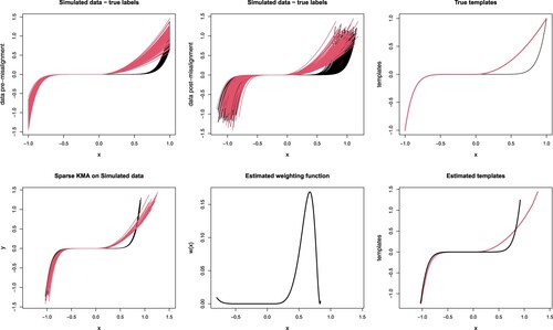
The generated data are shown in Figure 2, top-centre panel, each curve being coloured according to the true cluster label. It can be noticed that the curves in the 2 clusters are completely overlapped in the negative part of the abscissa, while the difference is evident in the positive part, and it becomes more and more evident towards the domain border. We thus expect to be able to capture this difference via $w\left(x\right)$, and we will verify whether the shape of the weighting function also reflects the between-cluster difference.

We fix the parameters of the sparseKMA procedure as follows: number of clusters K = 2 (K is set to the correct number of clusters because we will check the tuning of this parameter in the next section); tolerance for the stopping criterion tol = 0.001; sparsity parameter m = 0.4, and proportion of allowed warping $\mathrm{perc}=0.03,$ which are both fixed according to the general indications (see the discussion in Section 4.3).

The results of one run of sparseKMA are shown in Figure 2. The bottom-left panel shows the aligned curves coloured according to the estimated cluster labels in that run, and the result seems very good, since only 2 curves have been wrongly assigned. The curves are also very well aligned to their corresponding template, showing less residual variability than in their original pre-misalignment version, as shown in the panel above. The bottom-centre panel shows the final estimated $\tilde{w}\left(x\right)$, which correctly points out the relevant portion of the domain (evidently shown in the original data above), and the bottom-right panel shows the cluster templates, which are quite well estimated (if compared to the true templates in the panel above). The average misclassification rate over 20 runs of the procedure with 10 random starts was $0.2\mathrm{\%}$. One run of the procedure took on average ${35}^{\mathrm{\prime \prime }}$, and it was converging after 3 to 6 iterations, showing a quite good computational efficiency and stability of the optimisation. Initialisation of the algorithm was completely random.

4.2. Simulation 2: comparison with clustering and alignment, tuning of K

The purposes in this second simulation study are several. We first of all would like to test whether sparseKMA works in a more complex setting, where the portion of the domain differentiating among clusters is very limited. Moreover, we also aim at comparing the results to joint clustering and alignment (KMA) performed before sparse clustering (the strategy followed for analysing the growth curves in the Berkeley Growth Study in Floriello and Vitelli (2017), for instance), i.e. comparing to estimating phase variability first. Finally, we would like to check whether the proposed tuning strategy for selecting the number of groups effectively selects the correct K (for both sparseKMA and KMA). The data generation strategy for this second simulation is the following:

–	K = 2 for data generation, and n = 200 as before;
–	cluster true mean functions: $f_1^2\left(x\right)=q\cdot \sin \left(x\right)\cdot 1_{[0,2\pi ]}\left(x\right)$ and $f_2^2\left(x\right)=q\cdot [\sin (x)\cdot 1_{A^c}(x)+(\sqrt{3}-\sin \left(x\right))\cdot 1_A(x\left)\right],$ with $A=[\pi /3,2\pi /3]$ (see the left panel in Figure 3);
–	again, data $y_i\left(x\right)$ $(i=1,\dots ,n)$ are generated from the two mean functions $f_1^2\left(x\right)$ and $f_2^2\left(x\right)$ with a random parameter $q_i\sim N(1,{0.1}^2)$ (see the centre panel in Figure 3);
–	misaligned data are generated by warping the abscissa x via a curve specific affine warping $h_i\left(x\right)=a_i\cdot x+b_i,$ where $a_i$ and $b_i$ are generated in the same way as in Simulation 1, Section 4.1 (the resulting misaligned data are shown in the right panel in Figure 3).

Figure 3. One set of data generated for Simulation 2. Left panel, the true cluster templates; centre panel, synthetic curves coloured according to true labels, before misalignment; right panel, synthetic curves coloured according to true labels, after misalignment.

The parameters of the sparseKMA procedure are set as follows: tol = 0.001, perc = 0.03 (in line with the general indications of Section 4.3) and m = 0.03 (we choose the lowest reasonable value of m to ensure a fair comparison to KMA). The number K of groups is varied from 2 to 4, and tuned by looking at the boxplot of the within-cluster distances of the curves to the associated template, with the value at convergence of criterion (16(16) $\mathrm{wc}{d}^l=\sum _{k=1}^K\sum _{i\in C_k^l}{d}_w(f_i\circ h_i^l,{\phi }_k^l),$(16) ) overlapped in red. When setting the parameters of KMA, we used the same value of tol, but increased perc to 0.05, as the local search implemented in KMA benefits from a slightly larger threshold. KMA was run for $K=1,2,3,4,$ as KMA (differently from sparseKMA) can be run also for K = 1.

The results obtained via sparseKMA (for one run), in terms of the within-cluster distances, are shown in Figure 4, left panel: we see that sparseKMA correctly suggests 2 clusters, since the within-cluster distances do not evidently decrease when increasing the number of groups to more than 2 (p-value of the Mann-Whitney test for significant difference in the within-cluster distances when increasing from 2 to 3 groups was large in all runs). Figure 4 also shows (right panel) the same within-cluster distances after one run of KMA on the same data. These boxplots would suggest 4 clusters (at least) for KMA (p-value 0 for Mann-Whitney in all runs), thus confirming that a very localised amplitude grouping cannot be distinguished from the phase variability, so that KMA fails to select $K=2,$ and estimates an overly complex grouping structure.

Figure 4. Boxplots of the within-cluster distances to the cluster template for one run of Simulation 2, when varying the number of groups. Left panel, sparseKMA; right panel, KMA.

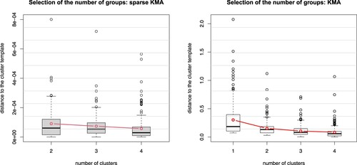
Figure 4 has lead us to conclude that there is an evident difference in performance of sparseKMA when compared to KMA, since the latter procedure seems to fail at selecting the correct number of groups. We will now inspect whether, when fixing $K=2,$ sparseKMA also shows an improved performance in terms of detecting the true groups. First of all, the average misclassification rate over 20 runs of sparseKMA was 1.274% when setting K = 2, while it was nearly 35% for KMA. Moreover, if we look at the final result of one of the runs, as shown in Figure 5, it is evident that the non-sparse KMA procedure fails at clustering the data because the difference among groups is too much localised in the domain: the data clustered and aligned by sparseKMA (left panel) reflect the true grouping structure, while KMA aligns well but fails at clustering (centre panel). This is also reflected in the templates estimated via the two procedures, much closer to the truth for sparseKMA (Figure 5, top-right) than for KMA (Figure 5, bottom-right).

Figure 5. Results of one of the runs of Simulation 2, when K = 2. Left panel, aligned data via sparseKMA, coloured according to the estimated cluster labels; centre panel, aligned data via KMA, coloured according to the estimated cluster labels; the 2 right panels show the templates estimated via sparseKMA (top) and KMA (bottom).

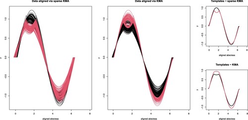
In the light of the results of Simulation 2, we can conclude that joint sparse clustering and alignment improves quite substantially the clustering results, particularly when the amplitude difference among clusters is localised in the domain. Clustering and alignment alone fails to correctly estimate the templates in the relevant portion of the domain, and thus misclassifies quite heavily the data. Moreover, as is evident from comparison of the left and centre panels in Figure 5, when using a join sparse clustering and alignment procedure it is possible to attain the same alignment of the data as that resulting from non-sparse clustering and alignment. And finally, clustering and alignment alone also overestimates the number of groups, which might be the result of not decoupling correctly phase and amplitude variability in this complex scenario. All in all, we thus conclude that jointly performing sparse clustering and alignment improves the final result of the analysis.

4.3. Simulation 3: tuning the parameters of sparseKMA

Aim of the third simulation study is to explore the effect of the two most important tuning parameters of sparseKMA: the sparsity parameter, m, and the parameter controlling the local search in the alignment procedure, perc (shortly named ‘alignment parameter’ hereafter). Specifically, we will test the algorithm performance when varying the true sparsity and misalignment level, and we will try to provide general indications for tuning the sparsity and the alignment parameters in practical situations.

The data generation mechanism is as follows:

–	number of classes K = 2, both for data generation and for clustering;
–	100 observations per class, thus n = 200 data in each scenario;
–	cluster true mean functions $f_1^3\left(x\right)=q\ast \sin \left(2\mathrm{\pi x}\right)\cdot 1_{[0,1]}\left(x\right)$ and $f_2^3\left(x\right)=q\ast \sin \left(2\mathrm{\pi x}\right)\cdot 1_{[0,m_{\mathrm{true}}]}\left(x\right)+q\ast \sin \left(2\pi m_{\mathrm{true}}\right)\cdot 1_{(m_{\mathrm{true}},1]}\left(x\right)$ for q = 3, and for varying values of $m_{\mathrm{true}}\in \{0.3,0.45,0.6\},$ respectively corresponding to a low/moderate/extreme overlapping of the resulting two clusters;
–	data $y_i\left(x\right)$ $(i=1,\dots ,n)$ are generated from the two mean functions $f_1^3\left(x\right)$ and $f_2^3\left(x\right)$ with a random parameter $q_i\sim N(3,{0.4}^2)$;
–	finally, misaligned data are generated from $y_i\left(x\right)$ by warping the abscissa x via a curve specific affine warping $h_i\left(x\right)=a_i\cdot x+b_i,$ with $a_i\sim N(1,{\sigma }^2)$ and $b_i\sim N(0,{\sigma }^2)$, and for varying values of $\sigma \in \{0.06,0.08,0.1\},$ respectively corresponding to a low/moderate/extreme misalignment in the generated data.

Two parameters of the sparseKMA procedure are fixed and set as follows: tol = 0.001 and $K=2.$ When testing the tuning of m, the data generated with all three values of $m_{\mathrm{true}}$ and with $\sigma =0.08$ are used; several reasonable values of the sparsity parameter m are then tested: 0.2, 0.3, 0.4, 0.5, 0.6 and 0.7, while the alignment parameter perc is set to 0.035. When testing the tuning of perc, the data generated with all three values of σ and with $m_{\mathrm{true}}=0.6$ are used; the tested values of the alignment parameter perc are relatively small: $0.01,0.02,0.025,0.03,0.035,0.04,$ and 0.05, in order to balance the speed of convergence with the need for exploring the space. The sparsity parameter m is set for this latter set of simulations to 0.5, for being agnostic. Finally, for each generated dataset corresponding to a combination of true parameter values $m_{\mathrm{true}}$ and σ, sparseKMA is run 50 times for each tested value of the tuning parameters, with an average computing time of ${37}^{\mathrm{\prime \prime }}$ per run (comparable to what has been reported in Simulation 1, Section 4.1). Results are reported in terms of a measure of goodness of the clustering, the Classification Error Rate (CER) index (1 – Rand index), which equals 0 if the partitions agree perfectly, and 1 in case of complete disagreement (Rand 1971). For the simulation settings concerning the tuning of perc, the goodness of the final alignment is also inspected, as measured via the average within-cluster distance of aligned data from the assigned estimated cluster template.

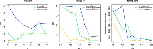
The results of this set of simulations are shown in Figure 6: from the average CER values shown in the left panel, obtained when tuning m, we see that sparseKMA performs generally well for low or moderate overlap between the groups, and that in such situations smaller values of m should be preferred; on the other hand, when the groups overlap substantially, the resulting clustering is generally worse unless m is set to 0.5 or more. Therefore, one can safely tune this parameter in the interval $[0.3,0.5],$ adjusting it to the specific data situation. Concerning the tuning of perc, Figure 6 shows that sparseKMA starts to perform well as soon as perc is large enough, both in terms of the CER index (centre panel) and of the average distance from the cluster template (right panel). We can notice that perc = 0.04 is already enough for attaining both good clustering and good alignment even when the level of misalignment is quite substantial. Moreover, even when the data are not so misaligned, the performance is robust to setting perc to larger values than the optimal (with the optimal value being around 0.02 both for good clustering and for good alignment). This leads us to conclude that setting perc to 0.03-0.04 would be a good choice in most settings.

Figure 6. Results of Simulation 3: average CER values (left and centre panels) and average distance to the cluster template (right panel) obtained over 50 runs of sparseKMA. Left panel: results obtained when testing several values of the sparsity parameter m, and when the true overlapping in the generated clusters is either low ($m_{\mathrm{true}}=0.3$), moderate ($m_{\mathrm{true}}=0.45$), or extreme ($m_{\mathrm{true}}=0.6$). Centre and right panels: results obtained when testing several values of the alignment parameter perc, and when the true misalignment level in the generated data is either low ($\sigma =0.06$), moderate ($\sigma =0.08$), or extreme ($\sigma =0.1$).

4.4. Simulation 4: robustness of sparseKMA to non-sparse clustering or no-misalignment

Aim of this final simulation study is to explore the robustness in the performance of sparseKMA to scenarios where this algorithm is not perfectly tuned to the data generating mechanism, either because the data grouping structure is not sparse with respect to the curves' domains, or because the curves are not misaligned.

In order to test the robustness to lack of misalignment, we used the same data generating process as in Simulation 3 (Section 4.3, with extreme cluster overlap), but we did not generate any misalignment in the curves' abscissa. We then run sparseKMA with the following parameter setting: $\mathrm{tol}=0.001,$ $K=2,$ and perc = 0.03 (as suggested in the parameter tuning study in Simulation 3, Section 4.3). In this setting, even when fixing a slightly too low value of the sparsity parameter $m=0.35,$ still the average CER over 50 runs of the algorithm is 0.12, with average misclassification rate of 0.065. When m = 0.6 as in the data generation, even if alignment is not needed the performance is extremely good, with CER = 0.095 and misclassification rate 0.05.

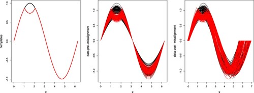
When instead aiming at testing the robustness to a non-sparse clustering of the curves, and in the presence of misalignment, we tested sparseKMA on the simulated scenario D from Sangalli et al. (2010b), as available in the package fdacluster (Sangalli, Secchi, Vantini, and Vitelli 2022) in R (R Core Team 2021). The original misaligned curves are shown in the left panel of Figure 7, coloured according to true labels; to further complicate the analysis, as is evident from the figure, a clustering is also present in the phase, thus creating a confusion on the correct amplitude grouping.

Figure 7. One run of sparseKMA on the data of Simulation 4. Left panel: original misaligned data from Scenario D in Sangalli et al. (2010b), coloured according to true labels; note that a clustering is also present in the phase. Right panel: curves aligned via sparseKMA with K = 2, coloured according to the estimated labels.

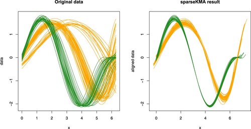
The results of the analysis via sparseKMA (same settings as above, apart from m = 0.1), as shown in the right panel of Figure 7 for one of the runs, indicate that the procedure is able to correctly cluster the curves even when the clustering is not sparse (the average CER obtained over 50 runs of sparseKMA is 0.003, with 94% of the runs resulting in CER=0). Not only, the curves are aligned to their corresponding cluster template with the same level of final alignment (left panel in Figure 7) as shown in the original simulations with KMA (see Figure 8 in Sangalli et al. (2010b), centre-left panel), which confirms that a joint sparse clustering and alignment procedure can attain the same level of alignment as a non-sparse one, even when the true clustering of the curves is not sparse.

5. Case study: the Berkeley growth study dataset

As illustrative example, we consider the Berkeley Growth Study, a very famous benchmark dataset for functional data analysis also provided in the fda package (Ramsay, Graves, and Hooker 2021) in R (R Core Team 2021). The analysis of the growth curves in the Berkeley dataset here reported should be considered as a follow-up to the analysis shown in Floriello and Vitelli (2017): in that paper, a sparse clustering procedure was used to detect a 2-groups classification on the set of growth velocities, after they had been aligned via KMA with K = 1. The very interesting result of that analysis was that sparse clustering was able to further cluster the data into 2 groups, essentially based on the presence/absence of the mid-spurt in the associated growth velocity curve (see Figure 7 in Floriello and Vitelli (2017)). This finding, together with the results obtained via KMA with K = 1 and reported in Sangalli et al. (2010a), showing a clear gender stratification in the estimated warping functions, would support the following conclusion: the Berkeley Growth Study curves show a gender grouping in the phase variability, a main amplitude feature (the main growth spurt, around 12 years of aligned age) common to all children, and a very localised amplitude clustering according to the presence/absence of the mid-spurt (between 2 and 5 years of aligned age). Aim of the present section is to confirm and validate these interesting findings via a unified procedure able to decouple the localised clustering in the amplitude from the phase variability, and possibly to gain more insight on this thoroughly-studied dataset.

The data in the Berkeley Growth Study consist in the heights (in cm) of 93 children, measured quarterly from 1 to 2 years, annually from 2 to 8 years and biannually from 8 to 18 years. The growth curves and derivatives are estimated, starting from such measurements, by means of monotonic cubic regression splines (Ramsay and Silverman 2005), and the growth velocities are further used in the analysis (see the top-left panel in Figure 8). Indeed, when looking at the growth velocities, the growth features shown by most children appear more evident (mainly the pubertal growth spurt around 12 years), but growth velocities also clearly show that each child follows her own biological clock. Using a sparse functional clustering procedure able to also account for such phase variability would then surely be beneficial.

The sparseKMA procedure is set as follows: we use the $L^2$ setting for coherence to Floriello and Vitelli (2017), and K = 2 to be able to compare the current findings with the ones reported in the previous paper. The sparsity parameter m is set to 0.5, to be able to capture the known localised amplitude features (mid-spurt). We set perc = 0.04 coherently to the conclusions of Simulation 3, Section 4.3, and tolerance for the iterative procedure to tol = 0.005, to ensure good convergence. Figure 8 shows, in the top panels, the original misaligned growth velocities (top-left) and the same growth velocities after running sparseKMA with the settings above (top-centre), when coloured according to the estimated cluster labels: the resulting clustering structure is essentially based on the presence or absence of the mid-spurt (3–5 years in aligned age), while the onset of the main growth velocity spurt (10–12 years in aligned age) seems mostly aligned across children. This feature distinguishing the clusters can be seen even more evidently in the estimated weighting function (bottom-left panel of Figure 8), that clearly points out as relevant part of the domain the mid-spurt onset, and with a much smaller peak the main growth velocity spurt. When inspecting the estimated cluster templates (bottom-centre panel of Figure 8), the mid-spurt in growth velocity is evidently present in the black cluster template, which shows two growth peaks, and absent in the red cluster template, which is nearly flat before the onset of the main pubertal spurt.

Even if we do not aim at performing any supervised classification of boys and girls, we recognise that gender plays a key role in shaping the kids' growth patterns, mainly in timing their biological clocks. Therefore, we would like to recognise this pattern in the estimated phase variability. The two right-most panels in Figure 8 explore the relationship between gender stratification and phase/amplitude variability in this dataset: in the top-right panel of Figure 8, the same growth velocities after alignment via sparseKMA as shown in the top-centre panel have been coloured in blue for boys (39 curves) and pink for girls (54 curves). No pattern is visible, and it looks like both boys and girls might show (or not show) a mid-spurt. Therefore, no gender stratification can be detected in the amplitude clusters. More interestingly, in the bottom-right panel of Figure 8 the estimated affine warping functions are coloured according to gender consistently to the panel above: this plot evidently shows that the gender stratification is present in the phase. Indeed, most girls show larger slope and intercepts as compared to boys, coherently to the well-known biological knowledge stating that girls grow stochastically earlier and slower than boys. All these findings are completely coherent to what had previously been reported on the same dataset (Sangalli et al. 2010a, 2010b), with the added insight given by the localised amplitude grouping structure. To further confirm such conclusion, we can analyse the estimated grouping structure, and compare it to the one detected in Floriello and Vitelli (2017): the clusters detected via sparseKMA nearly completely coincide to those found in Floriello and Vitelli (2017), with only 7 curves out of 93 that are assigned differently. This result is quite striking, since it validates the localised amplitude features detected in Floriello and Vitelli (2017), but it combines those findings with a coherent decoupling of phase and amplitude variability.

6. Analysis of the ICA centrelines of the AneuRisk65 dataset

We illustrate here another possible application of interest for the sparse clustering and alignment method, i.e. the analysis of the AneuRisk65 dataset. The AneuRisk project (see https://statistics.mox.polimi.it/aneurisk/) was a large scientific endeavour aimed at studying how the cerebral vessel morphology could impact the pathogenesis of cerebral aneurysms. The AneuRisk65 dataset is based on a set of three-dimensional angiographic images taken from 65 subjects, hospitalised at Niguarda Hospital in Milan (Italy) from September 2002 to October 2005, who were suspected of being affected by cerebral aneurysm. From the angiographies of the 65 subjects, among other information, estimates of the ICA centrelines were obtained via three-dimensional free-knot regression splines (Sangalli et al. 2009b). The first derivatives $x^{\mathrm{\prime }}$, $y^{\mathrm{\prime }}$ and $z^{\mathrm{\prime }}$ of the estimated curves, already displayed and commented in Figure 1, show an evident phase variability related to the very different dimensions and proportions of the subjects' skulls. However, this variability is ancillar to the scope of the analysis, which is the investigation of a possible grouping structure in the curves' shapes, related to differences in the cerebral morphology across subjects. Therefore, joint clustering and alignment of these curves was already presented in several papers (Sangalli et al. 2010a, 2010b), and two different amplitude clusters were detected and associated to the aneurysm position along the ICA. One of the evident results of those analyses, moreover, was that the shape differences were mostly localised in a specific part of the domain, closer to the brain: hence, we aim here at verifying that the same decoupling of phase and amplitude variability can be detected via sparse clustering and alignment, when also managing to automatically select the part of the domain most relevant to the clustering scope.

For this application, we need to adapt the sparseKMA in several ways: first of all, we specify the sparse clustering and alignment variational problem (7(7) $\begin{array}{rl}\underset{w\in L^2\left(D\right),\{h_1,\dots ,h_n\}\in W,\{C_1,\dots ,C_K\}}{max}& {\int }_{D}w\left(x\right)g\left(f_1\right(h_1\left(x\right)),\dots ,f_n(h_n\left(x\right));\{C_1,\dots ,C_K\left\}\right)\mathrm{d}x,\\ \mathrm{subject}\mathrm{to}\Vert w\left(x\right){\Vert }_{L^2\left(D\right)}\le 1,& w\left(x\right)\ge 0\mu -\mathrm{a}.\mathrm{e}.,\mu \left(\{x\in D:w(x)=0\}\right)\ge m.\end{array}$(7) ) with the functional measure defined in (10(10) $\rho (f_1,f_2)=\frac{〈〈f_1,f_2〉{〉}_{H^1}}{|f_1{|}_{H^1}|f_2{|}_{H^1}}$(10) ), which is more suited for capturing the vessel morphology. This means that, as discussed in Section 2.4, the formulation of the variational problem will be based on the maximisation of the within-cluster similarity (11(11) $\begin{array}{rl}& g\left(f_1\right(h_1\left(x\right)),\dots ,f_n(h_n\left(x\right));\{C_1,\dots ,C_K\left\}\right)=\\ & =\sum _{k=1}^K\frac{1}{n_k}\sum _{i,j\in C_k}\{\frac{f_i^{\mathrm{\prime }}\left(h_i\right(x\left)\right)}{|f_i{|}_{H^1}}\cdot \frac{f_j^{\mathrm{\prime }}\left(h_j\right(x\left)\right)}{|f_j{|}_{H^1}}\cdot 1_{\left\{h_i^{-1}\right(D_i)\cap h_j^{-1}(D_j\left)\right\}}(x\left)\right\}+\\ & -\frac{1}{n}\sum _{i,j=1,i\ne j}^n\{\frac{f_i^{\mathrm{\prime }}\left(h_i\right(x\left)\right)}{|f_i{|}_{H^1}}\cdot \frac{f_j^{\mathrm{\prime }}\left(h_j\right(x\left)\right)}{|f_j{|}_{H^1}}\cdot 1_{\left\{h_i^{-1}\right(D_i)\cap h_j^{-1}(D_j\left)\right\}}(x\left)\right\}.\end{array}$(11) ), and not on the maximisation of the between-cluster distance (5(5) $\begin{array}{rl}& g\left(f_1\right(h_1\left(x\right)),\dots ,f_n(h_n\left(x\right));\{C_1,\dots ,C_K\left\}\right)=\\ & =\frac{1}{n}\sum _{i,j=1}^n\{{\left(f_i\right(h_i\left(x\right))-f_j(h_j\left(x\right)\left)\right)}^2\cdot \frac{1_{\left\{h_i^{-1}\right(D_i)\cap h_j^{-1}(D_j\left)\right\}}\left(x\right)}{\sqrt{\mu \left(h_i^{-1}\right(D_i)\cap h_j^{-1}(D_j\left)\right)}}\}\\ & -\sum _{k=1}^K\frac{1}{n_k}\sum _{i,j\in C_k}\{{\left(f_i\right(h_i\left(x\right))-f_j(h_j\left(x\right)\left)\right)}^2\cdot \frac{1_{\left\{h_i^{-1}\right(D_i)\cap h_j^{-1}(D_j\left)\right\}}\left(x\right)}{\sqrt{\mu \left(h_i^{-1}\right(D_i)\cap h_j^{-1}(D_j\left)\right)}}\},\end{array}$(5) ). Secondly, the curves are in this case multidimensional, since the statistical unit of the AneuRisk65 dataset is a function $f:\mathbb{R}\to {\mathbb{R}}^3$. Hence, the natural generalisation of the method to multidimensional curves will be used, i.e. the functional similarity in (10(10) $\rho (f_1,f_2)=\frac{〈〈f_1,f_2〉{〉}_{H^1}}{|f_1{|}_{H^1}|f_2{|}_{H^1}}$(10) ) will be defined as an average of the similarity along the three dimensions. Finally, as it is evident from a look at the curves in Figure 1, the curves' domains are very different: from the common starting point at the terminal bifurcation of the ICA, some curves are observed for quite long portions of the ICA towards the heart, while others are pretty short, and this uniquely depends on the scan position during the examination (i.e. this has nothing to do with the morphology). Therefore, we need a robust implementation for the estimation of the cluster-specific templates, because on the leftmost portion of the domain very few curves are observed. For this reason, we estimate the template over the domain identified by the union of the domains of the curves assigned to the cluster with the same estimation procedure as defined in Sangalli et al. (2010b), i.e. we use Loess, an adaptive fitting that keeps the variance as constant as possible along the abscissa (Hastie and Tibshirani 1990).

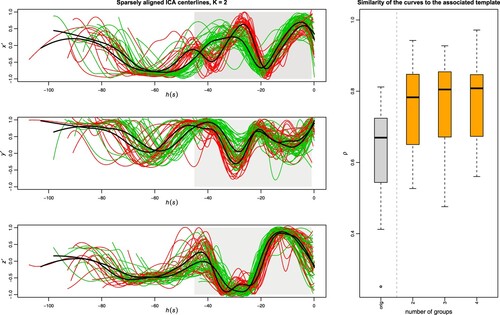
The sparseKMA procedure is set as follows: we vary K from 2 to 4 (more than 4 groups seems unreasonable given the sample size), and select the groups according to the elbow criterion as discussed in Section 3.2. The sparsity parameter m is set to 0.6, a much larger value than what used in previous applications of sparseKMA, and this is motivated by the particular characteristics of the ICA centrelines: due to the variation in the scan positioning, the size of the union of the curves' domains $|D|$ is much larger than that of the domains $D_i$ of many of the curves; therefore, and since m refers to the portion of D where w is null, a large value of m is advisable. The percentage of allowed warping is set to perc = 0.1 (since misalignment is quite extreme in this application), and the tolerance for the iterative procedure is tol = 0.01, slightly larger than in previous applications as the curves' variability is substantially and evidently larger. Figure 9 shows, in the right panel, the boxplot of the initial similarity of the misaligned curves to the overall template (as shown in Figure 1) in grey, and the final similarity of the aligned curves to the associated template after sparseKMA with K = 2, 3, 4 in orange: it is evident that, after an initial strong improvement, increasing the groups to more than 2 does not correspond in any increase of the within-cluster similarity. In the left panels of the same figure the aligned ICA centrelines after running sparseKMA with K = 2 are shown (from top to bottom, $x^{\mathrm{\prime }}$, $y^{\mathrm{\prime }}$ and $z^{\mathrm{\prime }}$), coloured according to the estimated cluster labels, and with grey background in the portion of the aligned domain where the final estimated $w(\cdot )$ is non-zero. The resulting cluster morphology and the 2 cluster templates show an astonishing coherence to the results shown in Sangalli et al. (2010b) (Figure 12, bottom-right panels): the template shapes are essentially the same, and the remaining within-cluster variability seems comparable. Not only, the grouping structure detected by KMA in Sangalli et al. (2010b) is indeed the same as detected here, with only 4 ICA centrelines being differently assigned, all corresponding to a non-aneurysm subject (which means that the reason for the different assignment might indeed be that these ICAs are ‘different’ in morphology in the rightmost part of the domain specifically). Finally, the portion of the domain selected from $w(\cdot )$ is essentially the same portion of the centrelines which was manually outlined in Sangalli et al. (2010b) (Figure 13) as the relevant one. For all these reasons, analysing the AnueRisk65 dataset via sparseKMA validates the previous findings, thus undoubtedly confirming the advantages of a jointly sparse procedure, which can enhance the interpretability of the final result without compromising the capability of decoupling phase and amplitude variability.

Figure 8. Results of sparseKMA on the Berkeley Growth Study data. Top-left, original growth velocities; top-centre, clustered and aligned growth velocities via sparseKMA with 2 clusters, coloured according to the estimated cluster labels; top-right, same as top-centre but coloured darker for boys and lighter for girls; bottom-left, estimated weighting function; bottom-centre, estimated templates, with labels colouring (as above); bottom-right, estimated warping functions, with gender colouring (as above).

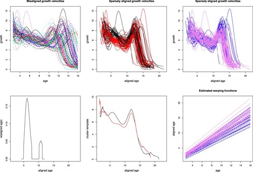
Figure 9. Results of sparseKMA on the AneuRisk65 dataset. Left panels, sparsely clustered and aligned first derivatives of the three-dimensional ICA centrelines (from top to bottom, $x^{\mathrm{\prime }}$, $y^{\mathrm{\prime }}$ and $z^{\mathrm{\prime }}$) via sparseKMA with 2 clusters, coloured according to the estimated cluster labels; the darker background area in the plot indicates the region of the domain where the weighting function is different from zero. Right panel, value of the functional measure of similarity between each ICA centreline and the associated template, for the original data (shown in Figure 1, first boxplot on the left), and for the sparsely aligned data with different Ks (three rightmost boxplots).

7. Conclusions and discussion of further developments

In this paper, a novel method for jointly performing sparse clustering and alignment of functional data was introduced and described in details, and its relevant mathematical properties were thoroughly discussed. Sparse clustering and alignment was then tested on simulated data, and its performance compared with a competitive approach. Finally, results obtained with this method on two case studies, the well-known growth curves from the Berkeley Growth Study and the AneuRisk65 dataset, were discussed in the light of previous findings. Sparse clustering and alignment is a completely novel methodological approach that fills a gap in the FDA literature on joint clustering and alignment. Results seem very promising, and the method showed to work pretty well even in the presence of a quite complex data structure. When compared to previous findings in the real case studies, novel interesting insights on the data were enlightened by the use of joint sparse clustering and alignment.

Nonetheless, the method is still in its infancy. First and foremost, a strategy for automatically tuning the sparsity parameter m would be beneficial, even if some general indications for its tuning have been provided in the context of Simulations (see Sections 4.3 and 4.4). A possible approach to automatic tuning would be the formal adaptation of the GAP statistics permutation-based strategy proposed in Floriello and Vitelli (2017) to work in case misalignment is present, which is surely a direction worth exploring in future research. Another approach, more targeted to the misalignment level observed in the data, could be computing some sufficient statistics describing phase and amplitude variation, and then relying on these for fixing m. This suggests a possible link between the optimal m for a given dataset, and the level of phase / amplitude variation in the data, which might be a very relevant direction for future research.

Secondly, even if the simulation studies described in Section 4 helped to gain understanding on the respective roles of the sparsity and alignment parameters, it looks like there could exist a trade-off between level of sparsity and goodness of alignment. Undoubtedly, a better understanding of the relationship between m and W would spread some light on this open aspect, as well. It is worth remarking here that changing the choice of W to a more complicated class than the one of strictly increasing affine transformations would also make the understanding of its relationship to m even more complex, not to mention the difficulties in keeping the mathematical formulation of the method rigorous.

Finally, another point that surely needs further inspection is the possible definition of sparse clustering and alignment in a homogeneous population of one cluster. Currently the method does not handle the limiting case when K = 1, because the weighting function w is not properly defined in this case. One easy fix, quite coherent from a purely theoretical standpoint, would be stating that sparse clustering and alignment degenerates into pure alignment when $K=1,$ as is the case for clustering and alignment with K = 1. However, one might then speculate whether the clustering might be present in the phase as well, and maybe in a sparse fashion. Therefore, it could be interesting to think of a generalisation of sparse clustering and alignment capable of estimating the grouping structure both in the amplitude and in the phase variability, with the possibility to use a specific sparsity constraint for each of the two clusterings.

Other future research directions include, but are not limited to: investigating the global convergence of the algorithm, and / or finding ways to tackle the variational problem (7(7) $\begin{array}{rl}\underset{w\in L^2\left(D\right),\{h_1,\dots ,h_n\}\in W,\{C_1,\dots ,C_K\}}{max}& {\int }_{D}w\left(x\right)g\left(f_1\right(h_1\left(x\right)),\dots ,f_n(h_n\left(x\right));\{C_1,\dots ,C_K\left\}\right)\mathrm{d}x,\\ \mathrm{subject}\mathrm{to}\Vert w\left(x\right){\Vert }_{L^2\left(D\right)}\le 1,& w\left(x\right)\ge 0\mu -\mathrm{a}.\mathrm{e}.,\mu \left(\{x\in D:w(x)=0\}\right)\ge m.\end{array}$(7) ) globally; developing a probabilistic approach to sparse clustering and alignment, for example by taking into account the point-wise curves density; and finally performing model-based clustering. All of these would lead to a nice paper in themselves, and are thus left to future speculation.

Implementation

The R package SparseFunClust implementing the method is on CRAN (Vitelli 2023). A repository on sparse clustering methods for functional data is continuously updated at https://github.com/valeriavitelli/SparseFunClust.

Disclosure statement

No potential conflict of interest was reported by the author(s).

Notes

1 The AneuRisk project is a scientific endeavour aimed at investigating the role of vessel morphology, blood fluid dynamics and biomechanical properties of the vascular wall, on the pathogenesis of cerebral aneurysms. The project has gathered together researchers of different scientific fields, ranging from neurosurgery and neuroradiology to statistics, numerical analysis and bio-engineering (see https://statistics.mox.polimi.it/aneurisk/ for details).

Appendix 1.

Proof of Proposition 1

Proof.

For proving that the metric $d_w(\cdot ,\cdot )$ in (9(9) $d_w(f_1,f_2)=\frac{1}{\sqrt{\mu (D_1\cap D_2)}}{\left({\int }_{D_1\cap D_2}w\right(x\left)\right(f_1\left(x\right)-f_2\left(x\right){)}^2\mathrm{d}x)}^{1/2},$(9) ) is W-invariant, we need to verify property (1(1) $d(f_1,f_2)=d(f_1\circ h,f_2\circ h),$(1) ). Take $f_1,f_2\in \mathcal{F}$ and $h\left(x\right)=\mathrm{ax}+b\in W$. Then $\begin{array}{rl}{d}_w(f_1\circ h,f_2\circ h)& =\frac{{\left({\int }_{h^{-1}(D_1\cap D_2)}w\right(h\left(x\right)\left)\right(f_1\left(h\right(x\left)\right)-f_2\left(h\right(x\left)\right){)}^2\mathrm{d}x)}^{1/2}}{\sqrt{\mu \left(h^{-1}\right(D_1\cap D_2\left)\right)}}\\ & =\frac{{\left({\int }_{D_1\cap D_2}w\right(y\left)\right(f_1\left(y\right)-f_2\left(y\right){)}^2\frac{\mathrm{d}y}{a})}^{1/2}}{\sqrt{{\int }_{h^{-1}(D_1\cap D_2)}\mathrm{d}x}}\\ & =\frac{{\left({\int }_{D_1\cap D_2}w\right(y\left)\right(f_1\left(y\right)-f_2\left(y\right){)}^2\mathrm{d}y)}^{1/2}\cdot \frac{1}{\sqrt{a}}}{\sqrt{{\int }_{D_1\cap D_2}\mathrm{d}y}\cdot \frac{1}{\sqrt{a}}}=d_w(f_1,f_2)\end{array}$where in the second line we used a change of variable defined by $y:=h\left(x\right),$ and the fact that in general $\mu \left(D\right)={\int }_D\mathrm{d}x.$

References

- Abramowicz, K., Arnqvist, P., Secchi, P., Luna, S.S.D., Vantini, S., and Vitelli, V. (2017), ‘Clustering Misaligned Dependent Curves Applied to Varved Lake Sediment for Climate Reconstruction’, Stochastic Environmental Research and Risk Assessment, 31, 71–85.
- Allen, G.I. (2013), ‘Sparse and Functional Principal Components Analysis’, arXiv preprint arXiv:1309.2895.
- Aneiros, G., and Vieu, P. (2014), ‘Variable Selection in Infinite-dimensional Problems’, Statistics & Probability Letters, 94, 12–20.
- Bauer, A., Scheipl, F., Küchenhoff, H., and Gabriel, A.A. (2021), ‘Registration for Incomplete Non-Gaussian Functional Data’, arXiv preprint arXiv:2108.05634.
- Bernardi, M., Canale, A., and Stefanucci, M. (2023), ‘Locally Sparse Function on Function Regression’, Journal of Computational and Graphical Statistics. https://doi.org/10.1080/10618600.2022.2130926.
- Berrendero, J.R., Cuevas, A., and Pateiro-López, B. (2016), ‘Shape Classification Based on Interpoint Distance Distributions’, Journal of Multivariate Analysis, 146, 237–247.
- Berrendero, J.R., Cuevas, A., and Torrecilla, J.L. (2016), ‘Variable Selection in Functional Data Classification: A Maxima-hunting Proposal’, Statistica Sinica, 26, 619–638.
- Centofanti, F., Lepore, A., and Palumbo, B. (2023), ‘Sparse and Smooth Functional Data Clustering’, Statistical Papers. https://doi.org/10.1007/s00362-023-01408-1.
- Chiou, J.M., and Li, P.L. (2007), ‘Functional Clustering and Identifying Substructures of Longitudinal Data’, Journal of the Royal Statistical Society: Series B (Statistical Methodology), 69, 679–699.
- Cremona, M.A., and Chiaromonte, F. (2023), ‘Probabilistic K-means with Local Alignment for Clustering and Motif Discovery in Functional Data’, Journal of Computational and Graphical Statistics. https://doi.org/10.1080/10618600.2022.2156522.
- Di, C.Z., Crainiceanu, C.M., Caffo, B.S., and Punjabi, N.M. (2009), ‘Multilevel Functional Principal Component Analysis’, The Annals of Applied Statistics, 3, 458.
- Di, C., Crainiceanu, C.M., and Jank, W.S. (2014), ‘Multilevel Sparse Functional Principal Component Analysis’, Stat, 3, 126–143.
- Elhamifar, E., and Vidal, R. (2013), ‘Sparse Subspace Clustering: Algorithm, Theory, and Applications’, IEEE Transactions on Pattern Analysis and Machine Intelligence, 35, 2765–2781.
- Floriello, D., and Vitelli, V. (2017), ‘Sparse Clustering of Functional Data’, Journal of Multivariate Analysis, 154, 1–18.
- Fraiman, R., Gimenez, Y., and Svarc, M. (2016), ‘Feature Selection for Functional Data’, Journal of Multivariate Analysis, 146, 191–208.
- Friedman, J.H., and Meulman, J.J. (2004), ‘Clustering Objects On a Subset of Attributes’, Journal of the Royal Statistical Society, Ser. B, 66, 815–849.
- Fu, S. (2019), ‘Clustering and Modelling of Phase Variation for Functional Data’, Ph.D. dissertation, University of British Columbia.
- Hastie, T., and Tibshirani, R. (1990), ‘Generalized Additive Models’, Monographs on Statistics and Applied Probability, 43, 335.
- Huang, J.Z., Shen, H., and Buja, A. (2009), ‘The Analysis of Two-way Functional Data Using Two-way Regularized Singular Value Decompositions’, Journal of the American Statistical Association, 104, 1609–1620.
- Jacques, J., and Preda, C. (2014), ‘Functional Data Clustering: a Survey’, Advances in Data Analysis and Classification, 8, 231–255.
- James, G.M., Hastie, T.J., and Sugar, C.A. (2000), ‘Principal Component Models for Sparse Functional Data’, Biometrika, 87, 587–602.
- James, G.M., Wang, J., and Zhu, J. (2009), ‘Functional Linear Regression that's Interpretable’, The Annals of Statistics, 37, 2083–2108.
- Kaufman, L., and Rousseeuw, P. (1990). Finding Groups in Data: An Introduction to Cluster Analysis, Hoboken, NJ: Wiley Series in Probability and Statistics.
- Kneip, A., and Ramsay, J.O. (2008), ‘Combining Registration and Fitting for Functional Models’, Journal of the American Statistical Association, 103, 1155–1165.
- Kneip, A., and Sarda, P. (2011), ‘Factor Models and Variable Selection in High-dimensional Regression Analysis’, The Annals of Statistics, 39, 2410–2447.
- Kraus, D. (2019), ‘Inferential Procedures for Partially Observed Functional Data’, Journal of Multivariate Analysis, 173, 583–603.
- Marron, J.S., Ramsay, J.O., Sangalli, L.M., and Srivastava, A. (2015), ‘Functional Data Analysis of Amplitude and Phase Variation’, Statistical Science, 30, 468–484.
- Mattar, M.A., Hanson, A.R., and Learned-Miller, E.G. (2012), ‘Unsupervised Joint Alignment and Clustering Using Bayesian Nonparametrics’, in UAI'12: Proceedings of the Twenty-Eighth Conference on Uncertainty in Artificial Intelligence, Arlington, VA: AUAI Press, pp. 584–593.
- McKeague, I.W., and Sen, B. (2010), ‘Fractals with Point Impact in Functional Linear Regression’, Annals of Statistics, 38, 2559.
- Müller, H.G., and Yang, W. (2010), ‘Dynamic Relations for Sparsely Sampled Gaussian Processes’, Test, 19, 1–29.
- Novo, S., Aneiros, G., and Vieu, P. (2019), ‘Fast Algorithm for Impact Point Selection in Semiparametric Functional Models’, in Multidisciplinary Digital Publishing Institute Proceedings (Vol. 21, 1st ed.), A Coruña, Spain: MDPI.
- Pini, A., and Vantini, S. (2016), ‘The Interval Testing Procedure: a General Framework for Inference in Functional Data Analysis’, Biometrics, 72, 835–845.
- Pini, A., and Vantini, S. (2017), ‘Interval-wise Testing for Functional Data’, Journal of Nonparametric Statistics, 29, 407–424.
- Pini, A., Vantini, S., Colosimo, B.M., and Grasso, M. (2018), ‘Domain-selective Functional Analysis of Variance for Supervised Statistical Profile Monitoring of Signal Data’, Journal of the Royal Statistical Society: Series C (Applied Statistics), 67, 55–81.
- Ramsay, J.O., Graves, S., and Hooker, G. (2021), Fda: Functional Data Analysis, R package version 5.5.1, https://CRAN.R-project.org/package=fda.
- Ramsay, J.O., and Silverman, B.W. (2005), Functional Data Analysis, New York, NY: Springer.
- Rand, W. (1971), ‘Objective Criteria for the Evaluation of Clustering Methods’, Journal of the American Statistical Association, 66, 846–850.
- R Core Team (2021), R: A Language and Environment for Statistical Computing, R Foundation for Statistical Computing, Vienna, Austria, https://www.R-project.org/.
- Sangalli, L.M., Secchi, P., Vantini, S., and Veneziani, A. (2009a), ‘A Case Study in Exploratory Functional Data Analysis: Geometrical Features of the Internal Carotid Artery’, Journal of the American Statistical Association, 104, 37–48.
- Sangalli, L.M., Secchi, P., Vantini, S., and Veneziani, A. (2009b), ‘Efficient Estimation of Three-dimensional Curves and Their Derivatives by Free-knot Regression Splines, Applied to the Analysis of Inner Carotid Artery Centrelines’, Journal of the Royal Statistical Society: Series C (Applied Statistics), 58, 285–306.
- Sangalli, L.M., Secchi, P., Vantini, S., and Vitelli, V. (2010a), ‘Functional Clustering and Alignment Methods with Applications’, Communications in Applied and Industrial Mathematics, 1, 205–224.
- Sangalli, L.M., Secchi, P., Vantini, S., and Vitelli, V. (2010b), ‘K-Mean Alignment for Curve Clustering’, Computational Statistics and Data Analysis, 54, 1219–1233.
- Sangalli, L., Secchi, P., Vantini, S., and Vitelli, V. (2022), fdacluster: Joint Clustering and Alignment of Functional Data, https://CRAN.R-project.org/package=fdacluster. R package version 0.1.1.
- Srivastava, A., and Klassen, E.P. (2016), Functional and Shape Data Analysis, New York, NY: Springer.
- Srivastava, A., Wu, W., Kurtek, S., Klassen, E., and Marron, J.S. (2011), ‘Registration of Functional Data using Fisher-Rao Metric’, arXiv preprint arXiv:1103.3817.
- Stefanucci, M., Sangalli, L.M., and Brutti, P. (2018), ‘PCA-based Discrimination of Partially Observed Functional Data, with An Application to AneuRisk65 Data Set’, Statistica Neerlandica, 72, 246–264.
- Tibshirani, R., and Walther, G. (2005), ‘Cluster Validation by Prediction Strength’, Journal of Computational and Graphical Statistics, 14, 511–528.
- Tuddenham, R.D. (1954), ‘Physical Growth of California Boys and Girls From Birth to Eighteen Years’, University of California Publications in Child Development, 1, 183–364.
- Vantini, S. (2012), ‘On the Definition of Phase and Amplitude Variability in Functional Data Analysis’, Test, 21, 676–696.
- Vitelli, V. (2023), SparseFunClust: Sparse Functional Clustering. https://cran.rproject.org/web/packages/SparseFunClust. R package version 1.0.0.
- Witten, D.M., and Tibshirani, R. (2010), ‘A Framework for Feature Selection in Clustering’, Journal of the American Statistical Association, 105, 713–726.
- Yao, F., Müller, H.G., and Wang, J.L. (2005), ‘Functional Data Analysis for Sparse Longitudinal Data’, Journal of the American Statistical Association, 100, 577–590.
- Yao, F., Wu, Y., and Zou, J. (2016), ‘Probability-enhanced Effective Dimension Reduction for Classifying Sparse Functional Data’, Test, 25, 1–22.
- Zeng, P., Qing Shi, J., and Kim, W.S. (2019), ‘Simultaneous Registration and Clustering for Multidimensional Functional Data’, Journal of Computational and Graphical Statistics, 28, 943–953.
- Zhang, Y., and Telesca, D. (2014), ‘Joint Clustering and Registration of Functional Data’, arXiv preprint arXiv:1403.7134.