Decomposition and reproducing property of local polynomial equivalent kernels in varying coefficient models

ABSTRACT

We consider local polynomial estimation for varying coefficient models and derive corresponding equivalent kernels that provide insights into the role of smoothing on the data and fill a gap in the literature. We show that the asymptotic equivalent kernels have an explicit decomposition with three parts: the inverse of the conditional moment matrix of covariates given the smoothing variable, the covariate vector, and the equivalent kernels of univariable local polynomials. We discuss finite-sample reproducing property which leads to zero bias in linear models with interactions between covariates and polynomials of the smoothing variable. By expressing the model in a centered form, equivalent kernels of estimating the intercept function are asymptotically identical to those of univariable local polynomials and estimators of slope functions are local analogues of slope estimators in linear models with weights assigned by equivalent kernels. Two examples are given to illustrate the weighting schemes and reproducing property.

KEYWORDS:

• Kronecker product
• linear model
• nonlinear interaction

MATHEMATICS SUBJECT CLASSIFICATION CODE:

• Primary 62G05
• secondary 62G08
• 62G20

1. Introduction

Motivated by situations of analysing complex data, several flexible regression models have been developed during the last three decades. Among these are the varying coefficient models (Hastie and Tibshirani 1993). They differ from classical linear models in that the regression coefficients are no longer constants but rather functions of a smoothing variable. The model has a form: (1) $Y=\sum _{g=1}^d{a}_g\left(U\right)X_g+ϵ=(1,\mathbf{x}{)}^T\mathbf{a}(U)+ϵ,$(1) where $\mathbf{x}=(X_2,\dots ,X_d{)}^T$ are continuous covariates, $X_1\equiv 1$, U is a continuous smoothing variable, $\mathbf{a}\left(U\right)=\left(a_1\right(U),\dots ,a_d(U){)}^T$ is the functional coefficient vector, and ε is the error term with $E(ϵ|U,\mathbf{x})=0$ and $\mathrm{Var}(ϵ|U,\mathbf{x})={\sigma }^2\left(U\right)$. When d = 1, model (1(1) $Y=\sum _{g=1}^d{a}_g\left(U\right)X_g+ϵ=(1,\mathbf{x}{)}^T\mathbf{a}(U)+ϵ,$(1) ) is reduced to a univariable nonparametric model. If the varying coefficients are constants, i.e. $a_g\left(U\right)=a_g,g=1,\dots ,d$, then (1(1) $Y=\sum _{g=1}^d{a}_g\left(U\right)X_g+ϵ=(1,\mathbf{x}{)}^T\mathbf{a}(U)+ϵ,$(1) ) is the multiple linear regression model. The model retains general nonparametric characteristics and allows nonlinear interactions between the smoothing variable U and covariates $\mathbf{x}$. Methods of estimating $\mathbf{a}(\cdot )$ include the local polynomial approach (Fan and Zhang 1999), smoothing splines (Hastie and Tibshirani 1993; Chiang, Rice, and Wu 2001), and penalised splines (Ruppert, Wand, and Carroll 2003). An overview on methodology of varying coefficient models is given in Fan and Zhang (2008) and Park, Mammen, Lee, and Lee (2015).

This paper focuses on the local polynomial approach. When d = 1, with local polynomial fitting of pth order, it is well known that the estimators are linear smoothers (linear in $Y_i$'s) and the associated equivalent kernels are available (Fan and Gijbels 1996). The equivalent kernels give insights into the role of kernel smoothing on the data and the corresponding estimator of $a_1(\cdot )$ has a remarkable ‘reproducing’ property (Tsybakov 2009, p:36), reproducing polynomials of degree $\le p$. However, to our knowledge, there are no results on equivalent kernels for local polynomial estimators in varying coefficient models (1(1) $Y=\sum _{g=1}^d{a}_g\left(U\right)X_g+ϵ=(1,\mathbf{x}{)}^T\mathbf{a}(U)+ϵ,$(1) ) in the literature. In this paper, we fill the gap by deriving asymptotically equivalent kernels for estimating $a_g(\cdot ),g=1,\dots ,d$ and their derivatives, providing explicit forms of the connections between equivalent kernels of general d and those of d = 1, and studying extension of the reproducing property. The contribution of our paper includes the following: (i) under some conditions, the asymptotic equivalent kernels corresponding to estimating $a_g^{\left(\nu \right)}(\cdot ),g=1,\dots ,d,\nu =0,\dots ,p$ in (1(1) $Y=\sum _{g=1}^d{a}_g\left(U\right)X_g+ϵ=(1,\mathbf{x}{)}^T\mathbf{a}(U)+ϵ,$(1) ) have explicit decomposition forms that connect to those of d = 1 (Theorem 3.2); (ii) the finite-sample equivalent kernels corresponding to estimating $a_g^{\left(\nu \right)}\left(u\right),g=1,\dots ,d,\nu =0,\dots ,p$ reproduce the νth derivative of polynomials of degree $\le p$ in u (Proposition 3.1); (iii) with centered covariates, estimators of $a_k(\cdot ),k=2,\dots ,d$ are local analogues of the slope estimators in linear models (Corollary 3.2).

We start the discussion with local linear fitting p = 1 and d = 2 in Theorem 3.1, followed by extending the results to a general d in (1(1) $Y=\sum _{g=1}^d{a}_g\left(U\right)X_g+ϵ=(1,\mathbf{x}{)}^T\mathbf{a}(U)+ϵ,$(1) ) with pth order local polynomial fitting in Theorem 3.2. Equations (16(16) $\begin{array}{rl}{K}_{g,\nu }^{\ast }(\frac{U_i-u_0}{h};X_{i2})& ={\zeta }_{g,\nu +1}^T{\left[{\mathrm{\Omega }}_2\right(u_0)\otimes {\mathcal{S}}_1]}^{-1}(\left[\begin{array}{c}1\\ X_{i2}\end{array}\right]\otimes \left[\begin{array}{c}1\\ \frac{U_i-u_0}{h}\end{array}\right])K\left(\frac{U_i-u_0}{h}\right)\\ & =e_{2,g}^T\left[{\mathrm{\Omega }}_2\right(u_0){]}^{-1}\left[\begin{array}{c}1\\ X_{i2}\end{array}\right]K_{\nu }^{\ast }\left(\frac{U_i-u_0}{h}\right)\\ & =\left({\tau }^{(g,1)}\right(u_0)+X_{i2}{\tau }^{(g,2)}(u_0\left)\right)(s^{(\nu +1,1)}+s^{(\nu +1,2)}((U_i-u_0)/h\left)\right)\\ & \times K\left(\frac{U_i-u_0}{h}\right)\end{array}$(16) ) and (26(26) $\begin{array}{rl}& K_{g,\nu }^{\ast }(\frac{U_i-u_0}{h};{\mathbf{x}}_{\left(i\right)}^T)={\zeta }_{g,\nu +1}^T\left({\mathrm{\Omega }}_d\right(u_0)\otimes {\mathcal{S}}_p{)}^{-1}({\tilde{\mathbf{x}}}_{\left(i\right)}\otimes {\mathcal{H}}_p^{-1}{\mathbf{u}}_{i0})K\left(\frac{U_i-u_0}{h}\right)\\ & =e_{d,g}^T\left[{\mathrm{\Omega }}_d\right(u_0){]}^{-1}{\tilde{\mathbf{x}}}_{\left(i\right)}^T{K}_{\nu }^{\ast }\left(\frac{U_i-u_0}{h}\right)\\ & =\left({\tau }^{(g,1)}\right(u_0)+\sum _{j=2}^d{X}_{\mathrm{ij}}{\tau }^{(g,j)}(u_0\left)\right)\left(\sum _{l=0}^p{\left(\frac{U_i-u_0}{h}\right)}^l{s}^{(\nu +1,l+1)}\right)K\left(\frac{U_i-u_0}{h}\right)\end{array}$(26) ) in Theorems 3.1 and 3.2 respectively show that there are direct connections between asymptotic equivalent kernels of (1(1) $Y=\sum _{g=1}^d{a}_g\left(U\right)X_g+ϵ=(1,\mathbf{x}{)}^T\mathbf{a}(U)+ϵ,$(1) ) and those of univariable local polynomial regression ((1(1) $Y=\sum _{g=1}^d{a}_g\left(U\right)X_g+ϵ=(1,\mathbf{x}{)}^T\mathbf{a}(U)+ϵ,$(1) ) with d = 1). It may be seen from the second equation in (26(26) $\begin{array}{rl}& K_{g,\nu }^{\ast }(\frac{U_i-u_0}{h};{\mathbf{x}}_{\left(i\right)}^T)={\zeta }_{g,\nu +1}^T\left({\mathrm{\Omega }}_d\right(u_0)\otimes {\mathcal{S}}_p{)}^{-1}({\tilde{\mathbf{x}}}_{\left(i\right)}\otimes {\mathcal{H}}_p^{-1}{\mathbf{u}}_{i0})K\left(\frac{U_i-u_0}{h}\right)\\ & =e_{d,g}^T\left[{\mathrm{\Omega }}_d\right(u_0){]}^{-1}{\tilde{\mathbf{x}}}_{\left(i\right)}^T{K}_{\nu }^{\ast }\left(\frac{U_i-u_0}{h}\right)\\ & =\left({\tau }^{(g,1)}\right(u_0)+\sum _{j=2}^d{X}_{\mathrm{ij}}{\tau }^{(g,j)}(u_0\left)\right)\left(\sum _{l=0}^p{\left(\frac{U_i-u_0}{h}\right)}^l{s}^{(\nu +1,l+1)}\right)K\left(\frac{U_i-u_0}{h}\right)\end{array}$(26) ) that the asymptotic equivalent kernels are decomposed into three main parts, the inverse of the conditional moment matrix of $(1,{\mathbf{x}}^{\mathrm{\top }}{)}^{\mathrm{\top }}$ given $U=u_0$, the covariate vector, and the equivalent kernels of univariable local polynomials. The finite-sample reproducing property is given in Proposition 3.1, which leads to zero bias when the true regression mean is the multiple linear model with interactions between $\mathbf{x}$ and up to order-p polynomials of U. In Section 3.3, we present two Corollaries of Theorems 3.1 and 3.2 when $\mathbf{x}$ is centered. It turns out that the centered form leads to simpler and more interpretable results: equivalent kernels of estimating $a_1^{\left(\nu \right)}(\cdot$) in (1(1) $Y=\sum _{g=1}^d{a}_g\left(U\right)X_g+ϵ=(1,\mathbf{x}{)}^T\mathbf{a}(U)+ϵ,$(1) ) with a general d is asymptotically identical to those of d = 1; estimators of $a_2^{\left(\nu \right)}(\cdot ),\dots ,a_d^{\left(\nu \right)}(\cdot )$ may be asymptotically expressed in a form analogous to the slope estimators in linear models with weights assigned by equivalent kernels. This interpretation appears to be new in the literature. We conjecture that these equivalent kernel results may be useful to develop methodology when the responses are random objects, i.e. Fréchet regression. Petersen and Müller (2019) propose to utilise the Euclidean local linear weights to fit Fréchet local linear regression. Thus Fréchet varying coefficient models will be an interesting topic for futureresearch.

The article is organised as follows. In Section 2, we summarise the local polynomial approach for estimating (1(1) $Y=\sum _{g=1}^d{a}_g\left(U\right)X_g+ϵ=(1,\mathbf{x}{)}^T\mathbf{a}(U)+ϵ,$(1) ) (Fan and Zhang 1999) and equivalent kernels of local polynomial regression (Fan and Gijbels 1996) with reproducing property in Proposition 2.1 (Tsybakov 2009). We present the main results in Section 3 and give two examples in Section 4 to illustrate, respectively, the weighting schemes of equivalent kernels when d = 2 and p = 1, and the reproducing property of equivalent kernels when d = 2 and p = 2. Proofs of Proposition 3.1 and Theorem 3.2 are provided in the Appendix.

2. Background

Consider a random sample $\left\{\right(Y_i,U_i,X_{i2},\dots ,X_{\mathrm{id}}),i=1,\dots ,n\}$ from model (1(1) $Y=\sum _{g=1}^d{a}_g\left(U\right)X_g+ϵ=(1,\mathbf{x}{)}^T\mathbf{a}(U)+ϵ,$(1) ) and define $X_{i1}=1,i=1,\dots ,n$. In this article, we adopt the local polynomial approach (Fan and Gijbels 1996) for estimating the coefficient functions $a_g(\cdot ),g=1,\dots ,d$ in (1(1) $Y=\sum _{g=1}^d{a}_g\left(U\right)X_g+ϵ=(1,\mathbf{x}{)}^T\mathbf{a}(U)+ϵ,$(1) ). For $U_i$ in a neighbourhood of a grid point $u_0$, $a_g\left(U_i\right)$ is approximated locally by a polynomial of order p, $\sum _{j=0}^p\left(a_g^{\left(j\right)}\right(u_0)/j!)(U_i-u_0{)}^j$ based on a Taylor expansion. Then estimation is carried out by weighted least squares (Fan and Zhang 1999): (2) $\underset{\text{β}}{min}\sum _{i=1}^n{(Y_i-\sum _{g=1}^d\left[\sum _{j=0}^p{\text{β}}_{g,j}\right(U_i-u_0{)}^j]X_{\mathrm{ig}})}^2{K}_h(U_i-u_0),$(2) where $\text{β}=({\text{β}}_{1,0},\dots ,{\text{β}}_{1,p},\dots ,{\text{β}}_{d,0},\dots ,{\text{β}}_{d,p}{)}^T$, $K(\cdot )$ is a symmetric probability density function, h is the bandwidth determining the size of local neighbourhood, and $K_h(\cdot )=K(\cdot /h)/h$. Throughout the paper, the dependence of β on $u_0$ and h is suppressed if no ambiguity results. Under some conditions, (2(2) $\underset{\text{β}}{min}\sum _{i=1}^n{(Y_i-\sum _{g=1}^d\left[\sum _{j=0}^p{\text{β}}_{g,j}\right(U_i-u_0{)}^j]X_{\mathrm{ig}})}^2{K}_h(U_i-u_0),$(2) ) has a unique solution, denoted by $\widehat{\text{β}}=({\widehat{\text{β}}}_{1,0},\dots ,{\widehat{\text{β}}}_{1,p},\dots ,{\widehat{\text{β}}}_{d,0},\dots ,{\widehat{\text{β}}}_{d,p}{)}^T$. It is clear that ${\widehat{\text{β}}}_{g,0}\left(u_0\right)$ estimates $a_g\left(u_0\right)$ of interest and $j!{\widehat{\text{β}}}_{g,j}\left(u_0\right)$ estimates the jth derivative $a_g^{\left(j\right)}\left(u_0\right)$. The expression (2(2) $\underset{\text{β}}{min}\sum _{i=1}^n{(Y_i-\sum _{g=1}^d\left[\sum _{j=0}^p{\text{β}}_{g,j}\right(U_i-u_0{)}^j]X_{\mathrm{ig}})}^2{K}_h(U_i-u_0),$(2) ) and its solution can be expressed in matrix notation. Let ${\mathbf{X}}_{u_0}=\left[\begin{array}{ccccccc}1& \cdots & (U_1-u_0{)}^p& \cdots & X_{1d}& \cdots & X_{1d}(U_1-u_0{)}^p\\ ⋮& & ⋮& \ddots & ⋮& \ddots & ⋮\\ 1& \cdots & (U_n-u_0{)}^p& \cdots & X_{\mathrm{nd}}& \cdots & X_{\mathrm{nd}}(U_n-u_0{)}^p\end{array}\right],$${\mathbf{W}}_{u_0}$ be an $n\times n$ diagonal matrix of weights $K_h(U_i-u_0)$, $i=1,\dots ,n$, and $\mathbf{y}=(Y_1,\dots ,Y_n{)}^T$. Then (2(2) $\underset{\text{β}}{min}\sum _{i=1}^n{(Y_i-\sum _{g=1}^d\left[\sum _{j=0}^p{\text{β}}_{g,j}\right(U_i-u_0{)}^j]X_{\mathrm{ig}})}^2{K}_h(U_i-u_0),$(2) ) can be expressed as $\underset{\text{β}}{min}(\mathbf{y}-{\mathbf{X}}_{u_0}\text{β}{)}^{\mathrm{\top }}{\mathbf{W}}_{u_0}(\mathbf{y}-{\mathbf{X}}_{u_0}\text{β})$ which yields (3) $\widehat{\text{β}}\left(u_0\right)=({\mathbf{X}}_{u_0}^T{\mathbf{W}}_{u_0}{\mathbf{X}}_{u_0}{)}^{-1}{\mathbf{X}}_{u_0}^T{\mathbf{W}}_{u_0}\mathbf{y}.$(3) The estimator of $\mathbf{a}\left(u_0\right)$ is (4) $\hat{\mathbf{a}}\left(u_0\right)=\left({\widehat{\text{β}}}_{1,0}\right(u_0),\dots ,{\widehat{\text{β}}}_{d,0}(u_0){)}^T=(I_d\otimes e_{p+1,1}^T\left)\widehat{\text{β}}\right(u_0),$(4) where ⊗ denotes the Kronecker product, $e_{p+1,k}$ is a column vector of length $(p+1)$ with 1 at the kth position and 0 elsewhere, and $I_d$ is the d-dimensional identity matrix. Let ${\zeta }_{g,\nu +1}$ be a column vector of length $d\times (p+1)$ with 1 at the $\left[\right(g-1)\times (p+1)+(\nu +1\left)\right]$th position and 0 elsewhere, $g=1,\dots ,d$, $\nu =0,\dots ,p$. Then ${\widehat{\text{β}}}_{g,\nu }\left(u_0\right)={\zeta }_{g,\nu +1}^T\widehat{\text{β}}\left(u_0\right)$. In other words, if ${\zeta }_{g,\nu +1}$ is partitioned into d groups of length $(p+1)$, then ${\zeta }_{g,\nu +1}$ indicates the $(\nu +1)$th position in the gth group, and ${\zeta }_{g,\nu +1}=e_{d,g}\otimes e_{p+1,\nu +1}$. In the special case of d = 1, ${\zeta }_{1,\nu +1}=e_{p+1,\nu +1}$.

The behaviour of $\widehat{\text{β}}\left(u_0\right)$ differs whether $u_0$ is an interior or boundary point. In this paper, we consider the case of interior points only. An informative tool to understand $\widehat{\text{β}}\left(u_0\right)$ is the equivalent kernel. For d = 1 in model (1(1) $Y=\sum _{g=1}^d{a}_g\left(U\right)X_g+ϵ=(1,\mathbf{x}{)}^T\mathbf{a}(U)+ϵ,$(1) ), the weight function $W_{\nu }(\cdot )$ for ${\widehat{\text{β}}}_{1,\nu }\left(u_0\right)$, i.e. ${\widehat{\text{β}}}_{1,\nu }\left(u_0\right)=\sum _{i=1}^n{W}_{\nu }\left(\right(U_i-u_0\left)/h\right)Y_i,\nu =0,\dots ,p$, is given as follows (Fan and Gijbels 1996, p:63): (5) $W_{\nu }\left(t\right)=e_{p+1,\nu +1}^T{S}_n^{-1}\{1,\mathrm{th},\dots ,(\mathrm{th}{)}^p{\}}^{T}K\left(t\right)/h,$(5) where $S_n={\mathbf{X}}_{u_0}^T{\mathbf{W}}_{u_0}{\mathbf{X}}_{u_0}$. For an interior point $u_0$, $W_{\nu }(\cdot )$ satisfies the following discrete moment conditions (Fan and Gijbels 1996, p:63 and p:103): (6) $\sum _{i=1}^n(U_i-u_0{)}^q{W}_{\nu }\left(\frac{U_i-u_0}{h}\right)={\delta }_{\nu ,q},0\le \nu ,q\le p,$(6) where ${\delta }_{\nu ,q}$ is an indicator function of $\{\nu =q\}$. For $\nu =0$, the expression (6(6) $\sum _{i=1}^n(U_i-u_0{)}^q{W}_{\nu }\left(\frac{U_i-u_0}{h}\right)={\delta }_{\nu ,q},0\le \nu ,q\le p,$(6) ) is referred to as the ‘reproducing’ property by Tsybakov (2009, p:36, Proposition 1.12) because ${\widehat{\text{β}}}_{1,0}(\cdot )$ reproduces polynomials of degree $\le p$. Here, we extend Tsybakov's statement to a general $\nu =0,\dots ,p,$ in the following Proposition, which shows that the local polynomial kernel approach has derivative reproducing property.

Proposition 2.1

Let $P(\cdot )$ be a polynomial of degree $\le p.$ Then (6(6) $\sum _{i=1}^n(U_i-u_0{)}^q{W}_{\nu }\left(\frac{U_i-u_0}{h}\right)={\delta }_{\nu ,q},0\le \nu ,q\le p,$(6) ) implies the reproducing property for $\nu =0,\dots ,p$: (7) $\nu !\sum _{i=1}^{n}P\left(U_i\right)W_{\nu }\left(\frac{U_i-u_0}{h}\right)=\frac{{\mathrm{d}}^{\nu }}{\mathrm{d}{u}^{\nu }}P\left(u\right){|}_{u=u_0}.$(7)

The proof of Proposition 2.1 is given in Tsybakov (2009, pp:36-37), is straightforward based on (6(6) $\sum _{i=1}^n(U_i-u_0{)}^q{W}_{\nu }\left(\frac{U_i-u_0}{h}\right)={\delta }_{\nu ,q},0\le \nu ,q\le p,$(6) ), and hence is omitted. For $\nu =1,\dots ,p,$ the reproducing property (7(7) $\nu !\sum _{i=1}^{n}P\left(U_i\right)W_{\nu }\left(\frac{U_i-u_0}{h}\right)=\frac{{\mathrm{d}}^{\nu }}{\mathrm{d}{u}^{\nu }}P\left(u\right){|}_{u=u_0}.$(7) ) means that the weight function $\nu !W_{\nu }(\cdot )$ corresponding to $\nu !{\widehat{\text{β}}}_{1,\nu }(\cdot )$ reproduces the νth derivative of polynomial $P(\cdot )$ with degree $\le p$. This includes shrinking polynomials of degree $<\nu$ to 0.

Let ${\mathcal{S}}_p=({\mu }_{i+j}{)}_{0\le i,j\le p}$ with ${\mu }_{i+j}$ being the $(i+j)$th moment of $K(\cdot )$. In an asymptotic form (Fan and Gijbels 1996, p:64), ${\widehat{\text{β}}}_{1,\nu }\left(u_0\right)=\left(1/\right(n{h}^{\nu +1}{f}_U\left(u_0\right))\times$ $\sum _{i=1}^n{K}_{\nu }^{\ast }\left(\right(U_i-u_0\left)/h\right)Y_i(1+o_p(1\left)\right),\nu =0,\dots ,p$, where $f_U(\cdot )$ is the density function of U and (8) $K_{\nu }^{\ast }\left(t\right)=e_{p+1,\nu +1}^T{\mathcal{S}}_p^{-1}(1,t,\dots ,t^p{)}^{T}K(t)=\left(\sum _{j=0}^p{t}^j{s}^{(\nu +1,j+1)}\right)K(t)$(8) with $s^{(i,j)}$ being the $(i,j)$th element of ${\mathcal{S}}_p^{-1}$. The $K_{\nu }^{\ast }(\cdot )$ is the asymptotic equivalent kernel for ${\widehat{\text{β}}}_{1,\nu }$, satisfying the following property (Fan and Gijbels 1996, p:64): (9) $\int t^q{K}_{\nu }^{\ast }\left(t\right)\mathrm{d}t={\delta }_{\nu ,q},0\le \nu ,q\le p,$(9) which is an asymptotic version of (6(6) $\sum _{i=1}^n(U_i-u_0{)}^q{W}_{\nu }\left(\frac{U_i-u_0}{h}\right)={\delta }_{\nu ,q},0\le \nu ,q\le p,$(6) ); that is, $K_{\nu }^{\ast }(\cdot )$ is a kernel of order $(\nu ,p+1)$ (see Gasser, Müller, and Mammitzsch 1985 for definition). It has been shown in Fan and Gijbels (1996) that local polynomials with $p-\nu =1$ outperform those with $p-\nu =0$ asymptotically.

In the next section, we derive the equivalent kernels of ${\widehat{\text{β}}}_{g,\nu }\left(u_0\right)$, $g=1,\dots ,d$, $\nu =0,\dots ,p$, for the varying coefficient model (1(1) $Y=\sum _{g=1}^d{a}_g\left(U\right)X_g+ϵ=(1,\mathbf{x}{)}^T\mathbf{a}(U)+ϵ,$(1) ), and investigate their reproducing property and connection to $K_{\nu }^{\ast }(\cdot )$ in (8(8) $K_{\nu }^{\ast }\left(t\right)=e_{p+1,\nu +1}^T{\mathcal{S}}_p^{-1}(1,t,\dots ,t^p{)}^{T}K(t)=\left(\sum _{j=0}^p{t}^j{s}^{(\nu +1,j+1)}\right)K(t)$(8) ).

3. Results

3.1. Local linear case with d = 2

For clarity of presentation, we start with a simple case when d = 2 and p = 1, i.e. (10) $Y=a_1\left(U\right)+a_2\left(U\right)X_2+ϵ.$(10) For a given interior point $u_0$, with p = 1, $S_n$ defined around (5(5) $W_{\nu }\left(t\right)=e_{p+1,\nu +1}^T{S}_n^{-1}\{1,\mathrm{th},\dots ,(\mathrm{th}{)}^p{\}}^{T}K\left(t\right)/h,$(5) ) is $S_n=\left[\begin{array}{cc}{\mathrm{△}}_{11}& {\mathrm{△}}_{12}\\ {\mathrm{△}}_{21}& {\mathrm{△}}_{22}\end{array}\right],\text{where}{\mathrm{△}}_{\mathrm{jk}}=\left[\begin{array}{cc}{S}_{\mathrm{jk}}^0& S_{\mathrm{jk}}^1\\ S_{\mathrm{jk}}^1& S_{\mathrm{jk}}^2\end{array}\right]$with $S_{\mathrm{jk}}^l=\sum _{i=1}^n{X}_{\mathrm{ij}}{X}_{\mathrm{ik}}(U_i-u_0{)}^l{K}_h(U_i-u_0)$. Under the model (10(10) $Y=a_1\left(U\right)+a_2\left(U\right)X_2+ϵ.$(10) ), based on (3(3) $\widehat{\text{β}}\left(u_0\right)=({\mathbf{X}}_{u_0}^T{\mathbf{W}}_{u_0}{\mathbf{X}}_{u_0}{)}^{-1}{\mathbf{X}}_{u_0}^T{\mathbf{W}}_{u_0}\mathbf{y}.$(3) ), ${\widehat{\text{β}}}_{g,\nu }\left(u_0\right)$, g = 1, 2 and $\nu =0,1$, is a linear smoother: (11) ${\widehat{\text{β}}}_{g,\nu }\left(u_0\right)=\sum _{i=1}^n{W}_{\nu }^g(\frac{U_i-u_0}{h};X_{i2})Y_i,$(11) where (12) $W_{\nu }^g(\frac{U_i-u_0}{h};X_{i2})={\zeta }_{g,\nu +1}^T{S}_n^{-1}(\left[\begin{array}{c}1\\ X_{i2}\end{array}\right]\otimes \left[\begin{array}{c}1\\ U_i-u_0\end{array}\right])K_h(U_i-u_0).$(12) It is straightforward to show that $W_{\nu }^g(\cdot ;\cdot )$ satisfies the following discrete moment conditions: for $\nu ,q=0,1$, g = 1, 2, (13) $\begin{array}{rl}& \sum _{i=1}^n(U_i-u_0{)}^q{W}_{\nu }^g(\frac{U_i-u_0}{h};X_{i2})={\delta }_{g,1}{\delta }_{\nu ,q};\\ & \sum _{i=1}^n{X}_{i2}(U_i-u_0{)}^q{W}_{\nu }^g(\frac{U_i-u_0}{h};X_{i2})={\delta }_{g,2}{\delta }_{\nu ,q}.\end{array}$(13) Equation (13(13) $\begin{array}{rl}& \sum _{i=1}^n(U_i-u_0{)}^q{W}_{\nu }^g(\frac{U_i-u_0}{h};X_{i2})={\delta }_{g,1}{\delta }_{\nu ,q};\\ & \sum _{i=1}^n{X}_{i2}(U_i-u_0{)}^q{W}_{\nu }^g(\frac{U_i-u_0}{h};X_{i2})={\delta }_{g,2}{\delta }_{\nu ,q}.\end{array}$(13) ) provides 4 moment conditions respectively for each combination of $(g,\nu )$. For g = 1, $W_{\nu }^1(\cdot ;\cdot )$, $\nu =0,1$, satisfies the same reproducing property as in Proposition 2.1 by the first equation in (13(13) $\begin{array}{rl}& \sum _{i=1}^n(U_i-u_0{)}^q{W}_{\nu }^g(\frac{U_i-u_0}{h};X_{i2})={\delta }_{g,1}{\delta }_{\nu ,q};\\ & \sum _{i=1}^n{X}_{i2}(U_i-u_0{)}^q{W}_{\nu }^g(\frac{U_i-u_0}{h};X_{i2})={\delta }_{g,2}{\delta }_{\nu ,q}.\end{array}$(13) ). In addition, by the second equation in (13(13) $\begin{array}{rl}& \sum _{i=1}^n(U_i-u_0{)}^q{W}_{\nu }^g(\frac{U_i-u_0}{h};X_{i2})={\delta }_{g,1}{\delta }_{\nu ,q};\\ & \sum _{i=1}^n{X}_{i2}(U_i-u_0{)}^q{W}_{\nu }^g(\frac{U_i-u_0}{h};X_{i2})={\delta }_{g,2}{\delta }_{\nu ,q}.\end{array}$(13) ), $W_{\nu }^1(\cdot ;\cdot )$ shrinks the covariate $X_{i2}$'s and interaction term $X_{i2}{U}_i$'s to 0. In other words, the equivalent kernels corresponding to estimating $a_1^{\left(\nu \right)}(\cdot )$ of d = 2 satisfy more properties than (6(6) $\sum _{i=1}^n(U_i-u_0{)}^q{W}_{\nu }\left(\frac{U_i-u_0}{h}\right)={\delta }_{\nu ,q},0\le \nu ,q\le p,$(6) ) of d = 1 case. For g = 2, we list the properties of $W_{\nu }^2(\cdot ;\cdot )$ in the following, while the general statement is given in Proposition 3.1 in Section 3.2.

For simplicity, denote $u_{i0}=(U_i-u_0)/h$. When g = 2, (13(13) $\begin{array}{rl}& \sum _{i=1}^n(U_i-u_0{)}^q{W}_{\nu }^g(\frac{U_i-u_0}{h};X_{i2})={\delta }_{g,1}{\delta }_{\nu ,q};\\ & \sum _{i=1}^n{X}_{i2}(U_i-u_0{)}^q{W}_{\nu }^g(\frac{U_i-u_0}{h};X_{i2})={\delta }_{g,2}{\delta }_{\nu ,q}.\end{array}$(13) ) gives the following results:

1. When $\nu =q=0$, $\sum _{i=1}^n{W}_0^2(u_{i0};X_{i2})=0$, i.e. shrinking constants to 0, and $\sum _{i=1}^n{X}_{i2}{W}_0^2(u_{i0};X_{i2})=1$, i.e. reproducing the first derivative with respect to $x_2$ $(\frac{\mathrm{\partial }}{\mathrm{\partial }{x}_2}{x}_2=1)$.

2. When $\nu =0,q=1$, $\sum _{i=1}^n(U_i-u_0)W_0^2(u_{i0};X_{i2})=0$ or $\sum _{i=1}^n{U}_i{W}_0^2(u_{i0};X_{i2})=0$, i.e. shrinking linear terms of $U_i$'s to 0; $\sum _{i=1}^n{X}_{i2}(U_i-u_0)W_0^2(u_{i0};X_{i2})=0$ or $\sum _{i=1}^n{X}_{i2}{U}_i{W}_0^2\left(\right(u_{i0};X_{i2})=u_0$, reproducing the first partial derivative with respect to $x_2$ $\left(\frac{\mathrm{\partial }}{\mathrm{\partial }{x}_2}\right(u{x}_2){|}_{u_0}=u_0)$.

3. When $\nu =1,q=0$, $\sum _{i=1}^n{W}_1^2(u_{i0};X_{i2})=0$ and $\sum _{i=1}^n{X}_{i2}{W}_1^2(u_{i0};X_{i2})=0$, shrinking constants and linear terms of $X_{i2}$'s to 0.

4. When $\nu =q=1$, $\sum _{i=1}^n(U_i-u_0)W_1^2(u_{i0};X_{i2})=0$ or $\sum _{i=1}^n{U}_i{W}_1^2(u_{i0};X_{i2})=0$, shrinking linear terms of $U_i$'s to 0; $\sum _{i=1}^n{X}_{i2}(U_i-u_0)W_1^2(u_{i0};X_{i2})=1$ or $\sum _{i=1}^n{X}_{i2}{U}_i{W}_1^2(u_{i0};X_{i2})=1$, reproducing the first partial derivative with respect to both $x_2$ and u $\left(\frac{{\mathrm{\partial }}^2}{\mathrm{\partial }u\mathrm{\partial }{x}_2}\right(u{x}_2){|}_{u_0}=1)$.

5. From 1–4 above, the finite-sample bias when estimating $E(Y|U,X_2)=b_0+b_{1}U+b_2{X}_2+b_{3}U{X}_2$ is zero.

Next we study the asymptotic forms for $W_{\nu }^g(\cdot ;\cdot )$, $\nu =0,1$ and g = 1, 2, to understand the local asymptotic behaviour of ${\widehat{\text{β}}}_{g,\nu }(\cdot )$. Let $\tilde{\mathbf{x}}=(1,X_2,\dots ,X_d{)}^{\mathrm{\top }}$, $f(x_2,\dots ,x_d|u)$ be the conditional density function of $\mathbf{x}$ given U = u, and ${\mathrm{\Omega }}_d\left(u\right)$ be the conditional expectation of $\tilde{\mathbf{x}}{\tilde{\mathbf{x}}}^T$ given U = u with its $(j,k)$th element $r_{\mathrm{jk}}\left(u\right)=E(X_j{X}_k|U=u)$, $j,k=1,\dots ,d$. Mimicking the derivations of (8(8) $K_{\nu }^{\ast }\left(t\right)=e_{p+1,\nu +1}^T{\mathcal{S}}_p^{-1}(1,t,\dots ,t^p{)}^{T}K(t)=\left(\sum _{j=0}^p{t}^j{s}^{(\nu +1,j+1)}\right)K(t)$(8) ) in Fan and Gijbels (1996) and using the asymptotic forms of $S_{\mathrm{jk}}^l$ in Zhang and Lee (2000, equation (5.2)), we obtain (14) $S_n^{-1}=\frac{1}{n{f}_U\left(u_0\right)}\left(\right[{\mathrm{\Omega }}_2\left(u_0\right){]}^{-1}\otimes {\mathcal{H}}_1^{-1}{\mathcal{S}}_1^{-1}{\mathcal{H}}_1^{-1})(1+O_p\left(\frac{\log n}{\sqrt{nh}}\right)),$(14) where ${\mathcal{H}}_p=\text{diag}(1,h,\dots ,h^p)$. It can be seen from (14(14) $S_n^{-1}=\frac{1}{n{f}_U\left(u_0\right)}\left(\right[{\mathrm{\Omega }}_2\left(u_0\right){]}^{-1}\otimes {\mathcal{H}}_1^{-1}{\mathcal{S}}_1^{-1}{\mathcal{H}}_1^{-1})(1+O_p\left(\frac{\log n}{\sqrt{nh}}\right)),$(14) ) that when $r_{12}\left(u_0\right)=r_{21}\left(u_0\right)=E(X_2|U=u_0)=0$, ${\mathrm{\Omega }}_2\left(u_0\right)$ is a diagonal matrix. The following theorem gives the explicit forms for the asymptotic equivalent kernel of ${\widehat{\text{β}}}_{g,\nu }\left(u_0\right)$ for g = 1, 2 and $\nu =0,1$, and provides their moment properties.

Theorem 3.1

Consider a random sample $\left\{\right(Y_i,U_i,X_{i2}),i=1,\dots ,n\}$ from model (10(10) $Y=a_1\left(U\right)+a_2\left(U\right)X_2+ϵ.$(10) ) (d = 2 in (1(1) $Y=\sum _{g=1}^d{a}_g\left(U\right)X_g+ϵ=(1,\mathbf{x}{)}^T\mathbf{a}(U)+ϵ,$(1) )) with local linear p = 1 estimators. For an interior point $u_0$, assume that $f\left(x_2|u_0\right)$ is bounded away from 0 and ∞ and has a compact support. Conditioned on $\{U_i,X_{i2}{\}}_{i=1}^n$ and under Conditions A in the Appendix, ${\widehat{\text{β}}}_{g,\nu }\left(u_0\right)$, g = 1, 2, $\nu =0,1$, has the following asymptotic form: (15) ${\widehat{\text{β}}}_{g,\nu }\left(u_0\right)=\frac{1}{n{h}^{\nu +1}{f}_U\left(u_0\right)}\sum _{i=1}^n{K}_{g,\nu }^{\ast }(\frac{U_i-u_0}{h};X_{i2})Y_i(1+o_p(1\left)\right),$(15) where the equivalent kernel (16) $\begin{array}{rl}{K}_{g,\nu }^{\ast }(\frac{U_i-u_0}{h};X_{i2})& ={\zeta }_{g,\nu +1}^T{\left[{\mathrm{\Omega }}_2\right(u_0)\otimes {\mathcal{S}}_1]}^{-1}(\left[\begin{array}{c}1\\ X_{i2}\end{array}\right]\otimes \left[\begin{array}{c}1\\ \frac{U_i-u_0}{h}\end{array}\right])K\left(\frac{U_i-u_0}{h}\right)\\ & =e_{2,g}^T\left[{\mathrm{\Omega }}_2\right(u_0){]}^{-1}\left[\begin{array}{c}1\\ X_{i2}\end{array}\right]K_{\nu }^{\ast }\left(\frac{U_i-u_0}{h}\right)\\ & =\left({\tau }^{(g,1)}\right(u_0)+X_{i2}{\tau }^{(g,2)}(u_0\left)\right)(s^{(\nu +1,1)}+s^{(\nu +1,2)}((U_i-u_0)/h\left)\right)\\ & \times K\left(\frac{U_i-u_0}{h}\right)\end{array}$(16) with ${\tau }^{(j,l)}\left(u_0\right)$ and $s^{(j,l)}$ the $(j,l)$th element of $\left[{\mathrm{\Omega }}_2\right(u_0){]}^{-1}$ and ${\mathcal{S}}_1^{-1}$ respectively. Then for $\nu ,q=0,1$, (17) $\begin{array}{rl}\int t^q(\int K_{g,\nu }^{\ast }(t;x_2\left)f\right(x_2|u_0\left)d{x}_2\right)\mathrm{d}t& ={\delta }_{g,1}{\delta }_{\nu ,q},\\ \int t^q(\int x_2{K}_{g,\nu }^{\ast }(t;x_2\left)f\right(x_2|u_0\left)d{x}_2\right)\mathrm{d}t& ={\delta }_{g,2}{\delta }_{\nu ,q},\end{array}$(17) which are the asymptotic counterparts of (13(13) $\begin{array}{rl}& \sum _{i=1}^n(U_i-u_0{)}^q{W}_{\nu }^g(\frac{U_i-u_0}{h};X_{i2})={\delta }_{g,1}{\delta }_{\nu ,q};\\ & \sum _{i=1}^n{X}_{i2}(U_i-u_0{)}^q{W}_{\nu }^g(\frac{U_i-u_0}{h};X_{i2})={\delta }_{g,2}{\delta }_{\nu ,q}.\end{array}$(13) ).

The results of Theorem 3.1 is a special case (d = 2, p = 1) of Theorem 3.2 and hence the proof of Theorem 3.1 follows that of Theorem 3.2. Expression (16(16) $\begin{array}{rl}{K}_{g,\nu }^{\ast }(\frac{U_i-u_0}{h};X_{i2})& ={\zeta }_{g,\nu +1}^T{\left[{\mathrm{\Omega }}_2\right(u_0)\otimes {\mathcal{S}}_1]}^{-1}(\left[\begin{array}{c}1\\ X_{i2}\end{array}\right]\otimes \left[\begin{array}{c}1\\ \frac{U_i-u_0}{h}\end{array}\right])K\left(\frac{U_i-u_0}{h}\right)\\ & =e_{2,g}^T\left[{\mathrm{\Omega }}_2\right(u_0){]}^{-1}\left[\begin{array}{c}1\\ X_{i2}\end{array}\right]K_{\nu }^{\ast }\left(\frac{U_i-u_0}{h}\right)\\ & =\left({\tau }^{(g,1)}\right(u_0)+X_{i2}{\tau }^{(g,2)}(u_0\left)\right)(s^{(\nu +1,1)}+s^{(\nu +1,2)}((U_i-u_0)/h\left)\right)\\ & \times K\left(\frac{U_i-u_0}{h}\right)\end{array}$(16) ) gives different decomposition forms of $K_{g,\nu }^{\ast }(\cdot ;\cdot )$ and interpretations of Theorem 3.1 are discussed as follows.

• From the first equation in (16(16) $\begin{array}{rl}{K}_{g,\nu }^{\ast }(\frac{U_i-u_0}{h};X_{i2})& ={\zeta }_{g,\nu +1}^T{\left[{\mathrm{\Omega }}_2\right(u_0)\otimes {\mathcal{S}}_1]}^{-1}(\left[\begin{array}{c}1\\ X_{i2}\end{array}\right]\otimes \left[\begin{array}{c}1\\ \frac{U_i-u_0}{h}\end{array}\right])K\left(\frac{U_i-u_0}{h}\right)\\ & =e_{2,g}^T\left[{\mathrm{\Omega }}_2\right(u_0){]}^{-1}\left[\begin{array}{c}1\\ X_{i2}\end{array}\right]K_{\nu }^{\ast }\left(\frac{U_i-u_0}{h}\right)\\ & =\left({\tau }^{(g,1)}\right(u_0)+X_{i2}{\tau }^{(g,2)}(u_0\left)\right)(s^{(\nu +1,1)}+s^{(\nu +1,2)}((U_i-u_0)/h\left)\right)\\ & \times K\left(\frac{U_i-u_0}{h}\right)\end{array}$(16) ), $K_{g,\nu }^{\ast }(\cdot ;\cdot )$ consists of three main parts: (i) inverse of the Kronecker product of conditional moments ${\mathrm{\Omega }}_2\left(u_0\right)$ and kernel moments ${\mathcal{S}}_1$, (ii) Kronecker product of covariate $(1,X_{i2}{)}^{\mathrm{\top }}$ and local linear term $(1,(U_i-u_0)/h{)}^{\mathrm{\top }}$, and (iii) kernel function $K(\cdot )$.

• For the second equation in (16(16) $\begin{array}{rl}{K}_{g,\nu }^{\ast }(\frac{U_i-u_0}{h};X_{i2})& ={\zeta }_{g,\nu +1}^T{\left[{\mathrm{\Omega }}_2\right(u_0)\otimes {\mathcal{S}}_1]}^{-1}(\left[\begin{array}{c}1\\ X_{i2}\end{array}\right]\otimes \left[\begin{array}{c}1\\ \frac{U_i-u_0}{h}\end{array}\right])K\left(\frac{U_i-u_0}{h}\right)\\ & =e_{2,g}^T\left[{\mathrm{\Omega }}_2\right(u_0){]}^{-1}\left[\begin{array}{c}1\\ X_{i2}\end{array}\right]K_{\nu }^{\ast }\left(\frac{U_i-u_0}{h}\right)\\ & =\left({\tau }^{(g,1)}\right(u_0)+X_{i2}{\tau }^{(g,2)}(u_0\left)\right)(s^{(\nu +1,1)}+s^{(\nu +1,2)}((U_i-u_0)/h\left)\right)\\ & \times K\left(\frac{U_i-u_0}{h}\right)\end{array}$(16) ), $K_{g,\nu }^{\ast }(\cdot ;\cdot )$ can be rewritten as a matrix product of (i) gth row of $\left[{\mathrm{\Omega }}_2\right(u_0){]}^{-1}$, (ii) covariate $(1,X_{i2}{)}^{\mathrm{\top }}$, and (iii) the equivalent kernel $K_{\nu }^{\ast }(\cdot )$ (8(8) $K_{\nu }^{\ast }\left(t\right)=e_{p+1,\nu +1}^T{\mathcal{S}}_p^{-1}(1,t,\dots ,t^p{)}^{T}K(t)=\left(\sum _{j=0}^p{t}^j{s}^{(\nu +1,j+1)}\right)K(t)$(8) ) of local linear regression. This expression shows the connection of $K_{g,\nu }^{\ast }(\cdot ;x_2)$ to $K_{\nu }^{\ast }(\cdot )$ in (8(8) $K_{\nu }^{\ast }\left(t\right)=e_{p+1,\nu +1}^T{\mathcal{S}}_p^{-1}(1,t,\dots ,t^p{)}^{T}K(t)=\left(\sum _{j=0}^p{t}^j{s}^{(\nu +1,j+1)}\right)K(t)$(8) ).

• It is clear that the $\nu !K_{1,\nu }^{\ast }(\cdot ;\cdot )$ for estimating $a_1^{\left(\nu \right)}(\cdot )$ under model (10(10) $Y=a_1\left(U\right)+a_2\left(U\right)X_2+ϵ.$(10) ) of d = 2 is different from (8(8) $K_{\nu }^{\ast }\left(t\right)=e_{p+1,\nu +1}^T{\mathcal{S}}_p^{-1}(1,t,\dots ,t^p{)}^{T}K(t)=\left(\sum _{j=0}^p{t}^j{s}^{(\nu +1,j+1)}\right)K(t)$(8) ) of d = 1. More explicitly, from (16(16) $\begin{array}{rl}{K}_{g,\nu }^{\ast }(\frac{U_i-u_0}{h};X_{i2})& ={\zeta }_{g,\nu +1}^T{\left[{\mathrm{\Omega }}_2\right(u_0)\otimes {\mathcal{S}}_1]}^{-1}(\left[\begin{array}{c}1\\ X_{i2}\end{array}\right]\otimes \left[\begin{array}{c}1\\ \frac{U_i-u_0}{h}\end{array}\right])K\left(\frac{U_i-u_0}{h}\right)\\ & =e_{2,g}^T\left[{\mathrm{\Omega }}_2\right(u_0){]}^{-1}\left[\begin{array}{c}1\\ X_{i2}\end{array}\right]K_{\nu }^{\ast }\left(\frac{U_i-u_0}{h}\right)\\ & =\left({\tau }^{(g,1)}\right(u_0)+X_{i2}{\tau }^{(g,2)}(u_0\left)\right)(s^{(\nu +1,1)}+s^{(\nu +1,2)}((U_i-u_0)/h\left)\right)\\ & \times K\left(\frac{U_i-u_0}{h}\right)\end{array}$(16) ), (18) $\begin{array}{rl}\widehat{\text{β}}\left(u_0\right)& =\sum _{i=1}^n\frac{[det({\mathrm{\Omega }}_2\left(u_0\right)){]}^{-1}}{n{f}_U\left(u_0\right)}\left[\begin{array}{c}{r}_{22}\left(u_0\right)-r_{12}\left(u_0\right)X_{i2}\\ h^{-1}{\mu }_2^{-1}\left(\right(U_i-u_0\left)/h\right)\left(r_{22}\right(u_0)-r_{12}(u_0\left)X_{i2}\right)\\ X_{i2}-r_{21}\left(u_0\right)\\ h^{-1}{\mu }_2^{-1}\left(\right(U_i-u_0\left)/h\right)(X_{i2}-r_{21}(u_0\left)\right)\end{array}\right]\\ & \times K_h(U_i-u_0)Y_i(1+o_p(1\left)\right).\end{array}$(18) Based on (18(18) $\begin{array}{rl}\widehat{\text{β}}\left(u_0\right)& =\sum _{i=1}^n\frac{[det({\mathrm{\Omega }}_2\left(u_0\right)){]}^{-1}}{n{f}_U\left(u_0\right)}\left[\begin{array}{c}{r}_{22}\left(u_0\right)-r_{12}\left(u_0\right)X_{i2}\\ h^{-1}{\mu }_2^{-1}\left(\right(U_i-u_0\left)/h\right)\left(r_{22}\right(u_0)-r_{12}(u_0\left)X_{i2}\right)\\ X_{i2}-r_{21}\left(u_0\right)\\ h^{-1}{\mu }_2^{-1}\left(\right(U_i-u_0\left)/h\right)(X_{i2}-r_{21}(u_0\left)\right)\end{array}\right]\\ & \times K_h(U_i-u_0)Y_i(1+o_p(1\left)\right).\end{array}$(18) ), even when $X_2$ and U are independent ($r_{12}=E\left(X_2\right)$ and $r_{22}=E\left(X_2^2\right)$ are free of $u_0$), $K_{1,\nu }^{\ast }(\cdot ;\cdot )$ still involves $X_{i2}$'s. Thus a sufficient condition for the equivalent kernels $K_{1,\nu }^{\ast }(\cdot ;\cdot )$ to be identical to those in (8(8) $K_{\nu }^{\ast }\left(t\right)=e_{p+1,\nu +1}^T{\mathcal{S}}_p^{-1}(1,t,\dots ,t^p{)}^{T}K(t)=\left(\sum _{j=0}^p{t}^j{s}^{(\nu +1,j+1)}\right)K(t)$(8) ) of d = 1 is $r_{12}(\cdot )\equiv 0$. That is, given U, $X_2$ has a conditional mean of 0.

• For g = 1, 2, the equivalent kernels for estimating the first derivative $a_g^{\mathrm{\prime }}(\cdot )$ is connected to those for estimating $a_g(\cdot )$: $K_{g,1}^{\ast }(t;\cdot )={\mu }_2^{-1}t{K}_{g,0}^{\ast }(t;\cdot )$. This is analogous to $K_1^{\ast }\left(t\right)={\mu }_2^{-1}t{K}_0^{\ast }\left(t\right)$ when p = 1 in (8(8) $K_{\nu }^{\ast }\left(t\right)=e_{p+1,\nu +1}^T{\mathcal{S}}_p^{-1}(1,t,\dots ,t^p{)}^{T}K(t)=\left(\sum _{j=0}^p{t}^j{s}^{(\nu +1,j+1)}\right)K(t)$(8) ).

•  (17(17) $\begin{array}{rl}\int t^q(\int K_{g,\nu }^{\ast }(t;x_2\left)f\right(x_2|u_0\left)d{x}_2\right)\mathrm{d}t& ={\delta }_{g,1}{\delta }_{\nu ,q},\\ \int t^q(\int x_2{K}_{g,\nu }^{\ast }(t;x_2\left)f\right(x_2|u_0\left)d{x}_2\right)\mathrm{d}t& ={\delta }_{g,2}{\delta }_{\nu ,q},\end{array}$(17) ) involves the conditional density $f\left(x_2|u\right)$ and shows the moment property of $K_{g,\nu }^{\ast }(t;x_2)$ with respect to the conditional density when estimating $a_1^{\left(\nu \right)}(\cdot )$ and $a_2^{\left(\nu \right)}(\cdot )$ in (10(10) $Y=a_1\left(U\right)+a_2\left(U\right)X_2+ϵ.$(10) ).

Next we discuss the decomposition and reproducing property of equivalent kernels for model (1(1) $Y=\sum _{g=1}^d{a}_g\left(U\right)X_g+ϵ=(1,\mathbf{x}{)}^T\mathbf{a}(U)+ϵ,$(1) ) with general d and p.

3.2. The case with general d and p

Results in Theorem 3.1 and the reproducing property (13(13) $\begin{array}{rl}& \sum _{i=1}^n(U_i-u_0{)}^q{W}_{\nu }^g(\frac{U_i-u_0}{h};X_{i2})={\delta }_{g,1}{\delta }_{\nu ,q};\\ & \sum _{i=1}^n{X}_{i2}(U_i-u_0{)}^q{W}_{\nu }^g(\frac{U_i-u_0}{h};X_{i2})={\delta }_{g,2}{\delta }_{\nu ,q}.\end{array}$(13) ) are extended to general d and p in this subsection. For ease of notation, let ${\mathbf{u}}_{i0}=(1,U_i-u_0,\dots ,(U_i-u_0{)}^p{)}^{\mathrm{\top }}$, (19) $\mathbf{X}=\left[\begin{array}{cccc}1& X_{12}& \cdots & X_{1d}\\ ⋮& ⋮& \ddots & ⋮\\ 1& X_{n2}& \cdots & X_{\mathrm{nd}}\end{array}\right]=\left[\begin{array}{c}{\tilde{\mathbf{x}}}_{\left(1\right)}^T\\ ⋮\\ {\tilde{\mathbf{x}}}_{\left(n\right)}^T\end{array}\right]=\left[\begin{array}{cc}1& {\mathbf{x}}_{\left(1\right)}^T\\ ⋮& ⋮\\ 1& {\mathbf{x}}_{\left(n\right)}^T\end{array}\right],$(19) where ${\tilde{\mathbf{x}}}_{\left(i\right)}^{\mathrm{\top }}$ is the ith row vector of $\mathbf{X}$ and ${\mathbf{x}}_{\left(i\right)}=(X_{i2},\dots ,X_{\mathrm{id}}{)}^T$ without the intercept. For $0\le \nu \le p$ and $1\le g\le d$, ${\widehat{\text{β}}}_{g,\nu }\left(u_0\right)$ is written as (20) ${\widehat{\text{β}}}_{g,\nu }\left(u_0\right)=\sum _{i=1}^n{W}_{\nu }^g(\frac{U_i-u_0}{h};{\mathbf{x}}_{\left(i\right)}^T)Y_i,$(20) where the weight function $W_{\nu }^g(\cdot ;{\mathbf{x}}_{\left(i\right)}^{\mathrm{\top }})$ is (21) $W_{\nu }^g(\frac{U_i-u_0}{h};{\mathbf{x}}_{\left(i\right)}^T)={\zeta }_{g,\nu +1}^T{S}_n^{-1}({\tilde{\mathbf{x}}}_{\left(i\right)}\otimes {\mathbf{u}}_{i0})K_h(U_i-u_0)$(21) with ${\zeta }_{g,\nu +1}$ defined in Section 2. Based on (21(21) $W_{\nu }^g(\frac{U_i-u_0}{h};{\mathbf{x}}_{\left(i\right)}^T)={\zeta }_{g,\nu +1}^T{S}_n^{-1}({\tilde{\mathbf{x}}}_{\left(i\right)}\otimes {\mathbf{u}}_{i0})K_h(U_i-u_0)$(21) ), we show in the Appendix that $W_{\nu }^g(\cdot ;{\mathbf{x}}_{\left(i\right)}^T)$ (21(21) $W_{\nu }^g(\frac{U_i-u_0}{h};{\mathbf{x}}_{\left(i\right)}^T)={\zeta }_{g,\nu +1}^T{S}_n^{-1}({\tilde{\mathbf{x}}}_{\left(i\right)}\otimes {\mathbf{u}}_{i0})K_h(U_i-u_0)$(21) ) enjoys the following property analogous to (13(13) $\begin{array}{rl}& \sum _{i=1}^n(U_i-u_0{)}^q{W}_{\nu }^g(\frac{U_i-u_0}{h};X_{i2})={\delta }_{g,1}{\delta }_{\nu ,q};\\ & \sum _{i=1}^n{X}_{i2}(U_i-u_0{)}^q{W}_{\nu }^g(\frac{U_i-u_0}{h};X_{i2})={\delta }_{g,2}{\delta }_{\nu ,q}.\end{array}$(13) ): for $0\le \nu ,q\le p$, $2\le k\le d$, and $1\le g\le d$, (22) $\begin{array}{rl}& \sum _{i=1}^n(U_i-u_0{)}^q{W}_{\nu }^g(\frac{U_i-u_0}{h};{\mathbf{x}}_{\left(i\right)}^T)={\delta }_{g,1}{\delta }_{\nu ,q},\\ & \sum _{i=1}^n{X}_{\mathrm{ik}}(U_i-u_0{)}^q{W}_{\nu }^g(\frac{U_i-u_0}{h};{\mathbf{x}}_{\left(i\right)}^T)={\delta }_{g,k}{\delta }_{\nu ,q}.\end{array}$(22) We state the reproducing property of $W_{\nu }^g(\cdot ;{\mathbf{x}}_{\left(i\right)}^T)$ formally in the following Proposition.

Proposition 3.1

Let $P(\cdot )$ be a polynomial of degree $\le p$ and $Q(\cdot ,x_k)=x_{k}P(\cdot )$, $k=2,\dots ,d$. Then (22(22) $\begin{array}{rl}& \sum _{i=1}^n(U_i-u_0{)}^q{W}_{\nu }^g(\frac{U_i-u_0}{h};{\mathbf{x}}_{\left(i\right)}^T)={\delta }_{g,1}{\delta }_{\nu ,q},\\ & \sum _{i=1}^n{X}_{\mathrm{ik}}(U_i-u_0{)}^q{W}_{\nu }^g(\frac{U_i-u_0}{h};{\mathbf{x}}_{\left(i\right)}^T)={\delta }_{g,k}{\delta }_{\nu ,q}.\end{array}$(22) ) implies the reproducing property, for $\nu =0,\dots ,p$: (23) $\nu !\sum _{i=1}^{n}P\left(U_i\right)W_{\nu }^g(\frac{U_i-u_0}{h};{\mathbf{x}}_{\left(i\right)}^T)={\delta }_{g,1}\left(\frac{d^{\nu }}{d{u}^{\nu }}P\right(u\left){|}_{u=u_0}\right);$(23) for $k=2,\dots ,d$, (24) $\nu !\sum _{i=1}^{n}Q(U_i;X_{\mathrm{ik}})W_{\nu }^g(\frac{U_i-u_0}{h};{\mathbf{x}}_{\left(i\right)}^T)={\delta }_{g,k}\frac{\mathrm{\partial }}{\mathrm{\partial }{x}_k}\left(\frac{{\mathrm{\partial }}^{\nu }}{\mathrm{\partial }{u}^{\nu }}Q\right(u,x_k\left){|}_{u=u_0}\right).$(24)

The outline of the proof of Proposition 3.1 is given in the Appendix. Proposition 3.1 shows that the equivalent kernel $\nu !W_{\nu }^1(\cdot ;\cdot )$ for estimating $a_1^{\left(\nu \right)}(\cdot )$ reproduces the νth derivative of polynomials of $U_i$'s with degree $\le p$, while shrinking $Q(U_i;X_{\mathrm{ik}})$'s to 0. Moreover, based on (24(24) $\nu !\sum _{i=1}^{n}Q(U_i;X_{\mathrm{ik}})W_{\nu }^g(\frac{U_i-u_0}{h};{\mathbf{x}}_{\left(i\right)}^T)={\delta }_{g,k}\frac{\mathrm{\partial }}{\mathrm{\partial }{x}_k}\left(\frac{{\mathrm{\partial }}^{\nu }}{\mathrm{\partial }{u}^{\nu }}Q\right(u,x_k\left){|}_{u=u_0}\right).$(24) ), the equivalent kernel $\nu !W_{\nu }^k(\cdot ;\cdot )$, $k=2,\dots ,d$, for estimating $a_k^{\left(\nu \right)}(\cdot )$ reproduces the νth derivative of $a_k(\cdot )$ when $a_k(\cdot )$ is a polynomial with degree $\le p$. These results imply that the finite-sample bias when estimating $E(Y|U,X_2,\dots ,X_d)=\sum _{j=0}^p{b}_{1j}{U}^j+\sum _{k=2}^d\sum _{j=0}^p{b}_{\mathrm{kj}}{U}^j{X}_k$ is zero, and that the polynomial reproducing property in Proposition 2.1 with d = 1 is valid for the interaction terms of covariates $X_k$'s and pth order polynomials of U under (1(1) $Y=\sum _{g=1}^d{a}_g\left(U\right)X_g+ϵ=(1,\mathbf{x}{)}^T\mathbf{a}(U)+ϵ,$(1) ) with a general d.

Theorem 3.2 below gives the decomposition and moment property of asymptotic equivalent kernels for general d and p, which is an extension of Theorem 3.1.

Theorem 3.2

Consider a random sample $\left\{\right(Y_i,U_i,{\mathbf{x}}_{\left(i\right)}^T),i=1,\dots ,n\}$ from model (1(1) $Y=\sum _{g=1}^d{a}_g\left(U\right)X_g+ϵ=(1,\mathbf{x}{)}^T\mathbf{a}(U)+ϵ,$(1) ) with local pth order polynomial estimators, $p\ge 0$. For an interior point $u_0$, assume that $f(x_2,\dots ,x_d|u_0)$ is bounded away from 0 and ∞ and has a compact support. Conditioned on $\{U_i,{\mathbf{x}}_{\left(i\right)}^T{\}}_{i=1}^n$ and under Conditions A in the Appendix, ${\widehat{\text{β}}}_{g,\nu }\left(u_0\right)$ has the following asymptotic form for $0\le \nu \le p$ and $1\le g\le d$: (25) ${\widehat{\text{β}}}_{g,\nu }\left(u_0\right)=\frac{1}{n{h}^{\nu +1}{f}_U\left(u_0\right)}\sum _{i=1}^n{K}_{g,\nu }^{\ast }(\frac{U_i-u_0}{h};{\mathbf{x}}_{\left(i\right)}^T)Y_i(1+o_p(1\left)\right),$(25) where the equivalent kernel (26) $\begin{array}{rl}& K_{g,\nu }^{\ast }(\frac{U_i-u_0}{h};{\mathbf{x}}_{\left(i\right)}^T)={\zeta }_{g,\nu +1}^T\left({\mathrm{\Omega }}_d\right(u_0)\otimes {\mathcal{S}}_p{)}^{-1}({\tilde{\mathbf{x}}}_{\left(i\right)}\otimes {\mathcal{H}}_p^{-1}{\mathbf{u}}_{i0})K\left(\frac{U_i-u_0}{h}\right)\\ & =e_{d,g}^T\left[{\mathrm{\Omega }}_d\right(u_0){]}^{-1}{\tilde{\mathbf{x}}}_{\left(i\right)}^T{K}_{\nu }^{\ast }\left(\frac{U_i-u_0}{h}\right)\\ & =\left({\tau }^{(g,1)}\right(u_0)+\sum _{j=2}^d{X}_{\mathrm{ij}}{\tau }^{(g,j)}(u_0\left)\right)\left(\sum _{l=0}^p{\left(\frac{U_i-u_0}{h}\right)}^l{s}^{(\nu +1,l+1)}\right)K\left(\frac{U_i-u_0}{h}\right)\end{array}$(26) with ${\tau }^{(j,l)}\left(u_0\right)$ and $s^{(j,l)}$ the $(j,l)$th element of $\left[{\mathrm{\Omega }}_d\right(u_0){]}^{-1}$ and ${\mathcal{S}}_p^{-1}$ respectively. The moment property of $K_{g,\nu }^{\ast }(t;x_2,\dots ,x_d)$ is given below: (27) $\begin{array}{r}\int t^q(\int \cdots \int K_{1,\nu }^{\ast }(t;x_2,\dots ,x_d\left)f\right(x_2,\dots ,x_d|u_0)\mathrm{d}{x}_2\cdots \mathrm{d}{x}_d)\mathrm{d}t={\delta }_{g,1}{\delta }_{\nu ,q},\\ \int t^q(\int \cdots \int x_k{K}_{g,\nu }^{\ast }(t;x_2,\dots ,x_d\left)f\right(x_2,\dots ,x_d|u_0)\mathrm{d}{x}_2\cdots \mathrm{d}{x}_d)\mathrm{d}t={\delta }_{g,k}{\delta }_{\nu ,q},\end{array}$(27) where $k=2,\dots ,d$, and $q=0,\dots ,p$. (27(27) $\begin{array}{r}\int t^q(\int \cdots \int K_{1,\nu }^{\ast }(t;x_2,\dots ,x_d\left)f\right(x_2,\dots ,x_d|u_0)\mathrm{d}{x}_2\cdots \mathrm{d}{x}_d)\mathrm{d}t={\delta }_{g,1}{\delta }_{\nu ,q},\\ \int t^q(\int \cdots \int x_k{K}_{g,\nu }^{\ast }(t;x_2,\dots ,x_d\left)f\right(x_2,\dots ,x_d|u_0)\mathrm{d}{x}_2\cdots \mathrm{d}{x}_d)\mathrm{d}t={\delta }_{g,k}{\delta }_{\nu ,q},\end{array}$(27) ) is the asymptotic counterpart of (22(22) $\begin{array}{rl}& \sum _{i=1}^n(U_i-u_0{)}^q{W}_{\nu }^g(\frac{U_i-u_0}{h};{\mathbf{x}}_{\left(i\right)}^T)={\delta }_{g,1}{\delta }_{\nu ,q},\\ & \sum _{i=1}^n{X}_{\mathrm{ik}}(U_i-u_0{)}^q{W}_{\nu }^g(\frac{U_i-u_0}{h};{\mathbf{x}}_{\left(i\right)}^T)={\delta }_{g,k}{\delta }_{\nu ,q}.\end{array}$(22) ) and contains $(p+1)d$ conditions for each combination of $(g,\nu )$.

The proof of Theorem 3.2 is given in the Appendix. From (26(26) $\begin{array}{rl}& K_{g,\nu }^{\ast }(\frac{U_i-u_0}{h};{\mathbf{x}}_{\left(i\right)}^T)={\zeta }_{g,\nu +1}^T\left({\mathrm{\Omega }}_d\right(u_0)\otimes {\mathcal{S}}_p{)}^{-1}({\tilde{\mathbf{x}}}_{\left(i\right)}\otimes {\mathcal{H}}_p^{-1}{\mathbf{u}}_{i0})K\left(\frac{U_i-u_0}{h}\right)\\ & =e_{d,g}^T\left[{\mathrm{\Omega }}_d\right(u_0){]}^{-1}{\tilde{\mathbf{x}}}_{\left(i\right)}^T{K}_{\nu }^{\ast }\left(\frac{U_i-u_0}{h}\right)\\ & =\left({\tau }^{(g,1)}\right(u_0)+\sum _{j=2}^d{X}_{\mathrm{ij}}{\tau }^{(g,j)}(u_0\left)\right)\left(\sum _{l=0}^p{\left(\frac{U_i-u_0}{h}\right)}^l{s}^{(\nu +1,l+1)}\right)K\left(\frac{U_i-u_0}{h}\right)\end{array}$(26) ), the equivalent kernel for ${\widehat{\text{β}}}_{g,\nu }\left(u_0\right)$ has decomposition forms analogous to the case for d = 2 and p = 1 in Theorem 3.1, while (26(26) $\begin{array}{rl}& K_{g,\nu }^{\ast }(\frac{U_i-u_0}{h};{\mathbf{x}}_{\left(i\right)}^T)={\zeta }_{g,\nu +1}^T\left({\mathrm{\Omega }}_d\right(u_0)\otimes {\mathcal{S}}_p{)}^{-1}({\tilde{\mathbf{x}}}_{\left(i\right)}\otimes {\mathcal{H}}_p^{-1}{\mathbf{u}}_{i0})K\left(\frac{U_i-u_0}{h}\right)\\ & =e_{d,g}^T\left[{\mathrm{\Omega }}_d\right(u_0){]}^{-1}{\tilde{\mathbf{x}}}_{\left(i\right)}^T{K}_{\nu }^{\ast }\left(\frac{U_i-u_0}{h}\right)\\ & =\left({\tau }^{(g,1)}\right(u_0)+\sum _{j=2}^d{X}_{\mathrm{ij}}{\tau }^{(g,j)}(u_0\left)\right)\left(\sum _{l=0}^p{\left(\frac{U_i-u_0}{h}\right)}^l{s}^{(\nu +1,l+1)}\right)K\left(\frac{U_i-u_0}{h}\right)\end{array}$(26) ) involves higher orders of local polynomials and more covariates. Some interpretations about (26(26) $\begin{array}{rl}& K_{g,\nu }^{\ast }(\frac{U_i-u_0}{h};{\mathbf{x}}_{\left(i\right)}^T)={\zeta }_{g,\nu +1}^T\left({\mathrm{\Omega }}_d\right(u_0)\otimes {\mathcal{S}}_p{)}^{-1}({\tilde{\mathbf{x}}}_{\left(i\right)}\otimes {\mathcal{H}}_p^{-1}{\mathbf{u}}_{i0})K\left(\frac{U_i-u_0}{h}\right)\\ & =e_{d,g}^T\left[{\mathrm{\Omega }}_d\right(u_0){]}^{-1}{\tilde{\mathbf{x}}}_{\left(i\right)}^T{K}_{\nu }^{\ast }\left(\frac{U_i-u_0}{h}\right)\\ & =\left({\tau }^{(g,1)}\right(u_0)+\sum _{j=2}^d{X}_{\mathrm{ij}}{\tau }^{(g,j)}(u_0\left)\right)\left(\sum _{l=0}^p{\left(\frac{U_i-u_0}{h}\right)}^l{s}^{(\nu +1,l+1)}\right)K\left(\frac{U_i-u_0}{h}\right)\end{array}$(26) ) is given below:

• The second equation in (26(26) $\begin{array}{rl}& K_{g,\nu }^{\ast }(\frac{U_i-u_0}{h};{\mathbf{x}}_{\left(i\right)}^T)={\zeta }_{g,\nu +1}^T\left({\mathrm{\Omega }}_d\right(u_0)\otimes {\mathcal{S}}_p{)}^{-1}({\tilde{\mathbf{x}}}_{\left(i\right)}\otimes {\mathcal{H}}_p^{-1}{\mathbf{u}}_{i0})K\left(\frac{U_i-u_0}{h}\right)\\ & =e_{d,g}^T\left[{\mathrm{\Omega }}_d\right(u_0){]}^{-1}{\tilde{\mathbf{x}}}_{\left(i\right)}^T{K}_{\nu }^{\ast }\left(\frac{U_i-u_0}{h}\right)\\ & =\left({\tau }^{(g,1)}\right(u_0)+\sum _{j=2}^d{X}_{\mathrm{ij}}{\tau }^{(g,j)}(u_0\left)\right)\left(\sum _{l=0}^p{\left(\frac{U_i-u_0}{h}\right)}^l{s}^{(\nu +1,l+1)}\right)K\left(\frac{U_i-u_0}{h}\right)\end{array}$(26) ) shows that $K_{g,\nu }^{\ast }(\cdot ;\cdot )$ consists of three parts: (i) $\left[{\mathrm{\Omega }}_d\right(u_0){]}^{-1}$, the inverse of the conditional moment matrix of $\tilde{\mathbf{x}}$ given $U=u_0$, (ii) the covariate vector ${\tilde{\mathbf{x}}}_{\left(i\right)}^{\mathrm{\top }}$, and the equivalent kernels $K_{\nu }^{\ast }(\cdot )$ (8(8) $K_{\nu }^{\ast }\left(t\right)=e_{p+1,\nu +1}^T{\mathcal{S}}_p^{-1}(1,t,\dots ,t^p{)}^{T}K(t)=\left(\sum _{j=0}^p{t}^j{s}^{(\nu +1,j+1)}\right)K(t)$(8) ) of univariable local polynomials.

• The second equation in (26(26) $\begin{array}{rl}& K_{g,\nu }^{\ast }(\frac{U_i-u_0}{h};{\mathbf{x}}_{\left(i\right)}^T)={\zeta }_{g,\nu +1}^T\left({\mathrm{\Omega }}_d\right(u_0)\otimes {\mathcal{S}}_p{)}^{-1}({\tilde{\mathbf{x}}}_{\left(i\right)}\otimes {\mathcal{H}}_p^{-1}{\mathbf{u}}_{i0})K\left(\frac{U_i-u_0}{h}\right)\\ & =e_{d,g}^T\left[{\mathrm{\Omega }}_d\right(u_0){]}^{-1}{\tilde{\mathbf{x}}}_{\left(i\right)}^T{K}_{\nu }^{\ast }\left(\frac{U_i-u_0}{h}\right)\\ & =\left({\tau }^{(g,1)}\right(u_0)+\sum _{j=2}^d{X}_{\mathrm{ij}}{\tau }^{(g,j)}(u_0\left)\right)\left(\sum _{l=0}^p{\left(\frac{U_i-u_0}{h}\right)}^l{s}^{(\nu +1,l+1)}\right)K\left(\frac{U_i-u_0}{h}\right)\end{array}$(26) ) not only gives an explicit connection between $K_{g,\nu }^{\ast }(\cdot ;\cdot )$ and $K_{\nu }^{\ast }(\cdot )$, but also the product $\left[{\mathrm{\Omega }}_d\right(u_0){]}^{-1}{\tilde{\mathbf{x}}}_{\left(i\right)}^T$ is analogous to the form of slopes ($\left({\mathbf{X}}^{\mathrm{\top }}\mathbf{X}{)}^{-1}{\tilde{\mathbf{x}}}_{\left(i\right)}^T\right)$ in classical linear models.

• Based on the first equation in (26(26) $\begin{array}{rl}& K_{g,\nu }^{\ast }(\frac{U_i-u_0}{h};{\mathbf{x}}_{\left(i\right)}^T)={\zeta }_{g,\nu +1}^T\left({\mathrm{\Omega }}_d\right(u_0)\otimes {\mathcal{S}}_p{)}^{-1}({\tilde{\mathbf{x}}}_{\left(i\right)}\otimes {\mathcal{H}}_p^{-1}{\mathbf{u}}_{i0})K\left(\frac{U_i-u_0}{h}\right)\\ & =e_{d,g}^T\left[{\mathrm{\Omega }}_d\right(u_0){]}^{-1}{\tilde{\mathbf{x}}}_{\left(i\right)}^T{K}_{\nu }^{\ast }\left(\frac{U_i-u_0}{h}\right)\\ & =\left({\tau }^{(g,1)}\right(u_0)+\sum _{j=2}^d{X}_{\mathrm{ij}}{\tau }^{(g,j)}(u_0\left)\right)\left(\sum _{l=0}^p{\left(\frac{U_i-u_0}{h}\right)}^l{s}^{(\nu +1,l+1)}\right)K\left(\frac{U_i-u_0}{h}\right)\end{array}$(26) ), one alternative form of $\widehat{\text{β}}\left(u_0\right)$ gives another connection to the case of d = 1: $\begin{array}{rl}\widehat{\text{β}}\left(u_0\right)& =\sum _{i=1}^n\frac{1}{n{f}_U\left(u_0\right)}(\left(\right[{\mathrm{\Omega }}_d\left(u_0\right){]}^{-1}{\tilde{\mathbf{x}}}_{\left(i\right)})\otimes \left[{\mathcal{H}}_p^{-1}{\mathcal{S}}_p^{-1}{\mathcal{H}}_p^{-1}{\mathbf{u}}_{i0}\right])K_h(U_i-u_0)Y_i\\ & \times (1+o_p(1\left)\right),\end{array}$which reduces to the case in Section 2 when d = 1.

3.3. Centering covariates

For classical linear models, centering covariates is useful in interpreting the effects of covariates and the slope estimators via least squares are the same with or without centering. In this subsection, we explore an analogous centered form for (1(1) $Y=\sum _{g=1}^d{a}_g\left(U\right)X_g+ϵ=(1,\mathbf{x}{)}^T\mathbf{a}(U)+ϵ,$(1) ) and we show that the resulting asymptotic equivalent kernels for estimating $a_1(\cdot )$ are identical to $K_{\nu }^{\ast }(\cdot )$ in (8(8) $K_{\nu }^{\ast }\left(t\right)=e_{p+1,\nu +1}^T{\mathcal{S}}_p^{-1}(1,t,\dots ,t^p{)}^{T}K(t)=\left(\sum _{j=0}^p{t}^j{s}^{(\nu +1,j+1)}\right)K(t)$(8) ) of d = 1 case. Moreover, the varying coefficient model may be interpreted as locally multiple linear model with interactions.

Let ${\overline{X}}_k$ be the sample mean of kth covariate $\{X_{\mathrm{ik}}{\}}_{i=1}^n$, $k=2,\dots ,d$. Then rewrite model (1(1) $Y=\sum _{g=1}^d{a}_g\left(U\right)X_g+ϵ=(1,\mathbf{x}{)}^T\mathbf{a}(U)+ϵ,$(1) ) in terms of centered covariates for the ith observation, $i=1,\dots ,n$, (28) $Y_i=\left(a_1\right(U_i)+{\overline{X}}_2{a}_2(U_i)+\dots +{\overline{X}}_d{a}_d(U_i\left)\right)+\sum _{k=2}^d{a}_k\left(U_i\right)(X_{\mathrm{ik}}-{\overline{X}}_k)+{ϵ}_i.$(28) It is straightforward to observe that the coefficient functions $a_k(\cdot ),k=2,\dots ,d$, are the same whether the covariates are centered or not, while the intercept function $a_1(\cdot )$ will be different. For ease of notation, define $X_{\mathrm{ik}}^c\equiv X_{\mathrm{ik}}-{\overline{X}}_k$, $k=2,\dots ,d$, (29) $\left[\begin{array}{ccc}{X}_{12}-{\overline{X}}_2& \cdots & X_{1d}-{\overline{X}}_d\\ ⋮& \ddots & ⋮\\ X_{n2}-{\overline{X}}_2& \cdots & X_{\mathrm{nd}}-{\overline{X}}_d\end{array}\right]\equiv \left[\begin{array}{ccc}{X}_{12}^c& \cdots & X_{1d}^c\\ ⋮& \ddots & ⋮\\ X_{n2}^c& \cdots & X_{\mathrm{nd}}^c\end{array}\right]\equiv \left[\begin{array}{c}({\mathbf{x}}_{\left(1\right)}^c{)}^{\mathrm{\top }}\\ ⋮\\ ({\mathbf{x}}_{\left(n\right)}^c{)}^{\mathrm{\top }}\end{array}\right],$(29) and $(d-1)\times (d-1)$ matrix $M_{\mathrm{xx}}\left(u\right)$ with $(j-1,k-1)$th element being $E\left(X_{\mathrm{ij}}^c{X}_{\mathrm{ik}}^c|u\right)\equiv r_{\mathrm{jk}}^c\left(u\right)$, $j,k=2,\dots ,d$. When the conditional density of $X_k$ given U = u is well defined, $E\left(X_{\mathrm{ik}}|u\right)$ is a function of u and $E\left(X_{\mathrm{ik}}^c|u\right)=0$. The following Corollary for d = 2 and p = 1 is a special case of Theorem 3.1 either when $X_{i2}$'s are centered or when $E(X_2|U=u)=r_{12}\left(u\right)=0$.

Corollary 3.1

Under the conditions in Theorem 3.1, results (a) and (b) below hold when $X_{i2}$'s are centered.

(a)	$K_{1,\nu }^{\ast }(\cdot )$, $\nu =0,1$, is identical to $K_{\nu }^{\ast }(\cdot )$ in (8(8) $K_{\nu }^{\ast }\left(t\right)=e_{p+1,\nu +1}^T{\mathcal{S}}_p^{-1}(1,t,\dots ,t^p{)}^{T}K(t)=\left(\sum _{j=0}^p{t}^j{s}^{(\nu +1,j+1)}\right)K(t)$(8) ) and does not involve $X_{i2}^c$'s;
(b)	the form of $K_{2,\nu }^{\ast }(\cdot ;\cdot )$, $\nu =0,1$, becomes simpler:

(30) $\begin{array}{rl}{K}_{2,0}^{\ast }(\frac{U_i-u_0}{h};X_{i2}^c)& =\left(\frac{X_{i2}^c}{r_{22}^c\left(u_0\right)}\right)K\left(\frac{U_i-u_0}{h}\right),\\ K_{2,1}^{\ast }(\frac{U_i-u_0}{h};X_{i2}^c)& =\left(\frac{X_{i2}^c}{r_{22}^c\left(u_0\right)}\right)K_1^{\ast }\left(\frac{U_i-u_0}{h}\right)\\ & =\left(\frac{X_{i2}^c}{r_{22}^c\left(u_0\right)}\right)\left(\frac{U_i-u_0}{h{\mu }_2}\right)K\left(\frac{U_i-u_0}{h}\right)\\ & =\left(\frac{U_i-u_0}{h{\mu }_2}\right)K_{2,0}^{\ast }(\frac{U_i-u_0}{h};X_{i2}^c).\end{array}$(30)

(c)

When $E\left(X_2|u_0\right)=0$, the results in (a) and (b) hold without centering of $X_{i2}$'s, and $X_{i2}^c$ in (30(30) $\begin{array}{rl}{K}_{2,0}^{\ast }(\frac{U_i-u_0}{h};X_{i2}^c)& =\left(\frac{X_{i2}^c}{r_{22}^c\left(u_0\right)}\right)K\left(\frac{U_i-u_0}{h}\right),\\ K_{2,1}^{\ast }(\frac{U_i-u_0}{h};X_{i2}^c)& =\left(\frac{X_{i2}^c}{r_{22}^c\left(u_0\right)}\right)K_1^{\ast }\left(\frac{U_i-u_0}{h}\right)\\ & =\left(\frac{X_{i2}^c}{r_{22}^c\left(u_0\right)}\right)\left(\frac{U_i-u_0}{h{\mu }_2}\right)K\left(\frac{U_i-u_0}{h}\right)\\ & =\left(\frac{U_i-u_0}{h{\mu }_2}\right)K_{2,0}^{\ast }(\frac{U_i-u_0}{h};X_{i2}^c).\end{array}$(30) ) can be replaced by $X_{i2}$.

Corollary 3.1 shows that with $X_{i2}^c$'s, the equivalent kernels $K_{2,\nu }^{\ast }(\cdot ;\cdot )$, $\nu =0,1$ corresponding to ${\widehat{\text{β}}}_{2,0}\left(u_0\right)$ and ${\widehat{\text{β}}}_{2,1}\left(u_0\right)$ respectively involve a factor $X_{i2}^c/r_{22}^c\left(u_0\right)$. In addition, when $X_2$ and U are independent, $r_{22}^c$ is a constant free of $u_0$, and further adopting standardised $X_{i2}$ in (28(28) $Y_i=\left(a_1\right(U_i)+{\overline{X}}_2{a}_2(U_i)+\dots +{\overline{X}}_d{a}_d(U_i\left)\right)+\sum _{k=2}^d{a}_k\left(U_i\right)(X_{\mathrm{ik}}-{\overline{X}}_k)+{ϵ}_i.$(28) ) by $X_{i2}^{\mathrm{std}}=X_{i2}^c/\sqrt{r_{22}^c}$, $i=1,\dots ,n$, leads to $K_{2,\nu }^{\ast }\left(\right(U_i-u_0)/h;X_{i2}^{\mathrm{std}})=X_{i2}^{\mathrm{std}}{K}_{1,\nu }^{\ast }\left(\right(U_i-u_0\left)/h\right)$, $\nu =0,1$.

Let us further explore Corollary 3.1 by centering $Y_i$'s as well, denoted by $Y_i^c$. With centered observations $\left\{\right(Y_i^c,U_i,X_{i2}^c),i=1\dots ,n\}$, and based on (30(30) $\begin{array}{rl}{K}_{2,0}^{\ast }(\frac{U_i-u_0}{h};X_{i2}^c)& =\left(\frac{X_{i2}^c}{r_{22}^c\left(u_0\right)}\right)K\left(\frac{U_i-u_0}{h}\right),\\ K_{2,1}^{\ast }(\frac{U_i-u_0}{h};X_{i2}^c)& =\left(\frac{X_{i2}^c}{r_{22}^c\left(u_0\right)}\right)K_1^{\ast }\left(\frac{U_i-u_0}{h}\right)\\ & =\left(\frac{X_{i2}^c}{r_{22}^c\left(u_0\right)}\right)\left(\frac{U_i-u_0}{h{\mu }_2}\right)K\left(\frac{U_i-u_0}{h}\right)\\ & =\left(\frac{U_i-u_0}{h{\mu }_2}\right)K_{2,0}^{\ast }(\frac{U_i-u_0}{h};X_{i2}^c).\end{array}$(30) ), (31) ${\widehat{\text{β}}}_{2,0}\left(u_0\right)=\left[\frac{n^{-1}\sum _{i=1}^n{X}_{i2}^c{Y}_i^c{K}_h(U_i-u_0)}{r_{22}^c\left(u_0\right)f_U\left(u_0\right)}\right](1+o_p(1\left)\right).$(31) The denominator in (31(31) ${\widehat{\text{β}}}_{2,0}\left(u_0\right)=\left[\frac{n^{-1}\sum _{i=1}^n{X}_{i2}^c{Y}_i^c{K}_h(U_i-u_0)}{r_{22}^c\left(u_0\right)f_U\left(u_0\right)}\right](1+o_p(1\left)\right).$(31) ) can be viewed as a local variance of $X_2$ at $u_0$, while the numerator in (31(31) ${\widehat{\text{β}}}_{2,0}\left(u_0\right)=\left[\frac{n^{-1}\sum _{i=1}^n{X}_{i2}^c{Y}_i^c{K}_h(U_i-u_0)}{r_{22}^c\left(u_0\right)f_U\left(u_0\right)}\right](1+o_p(1\left)\right).$(31) ) can be interpreted as the locally weighted sample covariance between $X_{i2}$'s and $Y_i$'s with weights assigned by $K_h(U_i-u_0)$ around $u_0$, denoted by ${\widehat{\text{Cov}}}_{u_0}(X_2,Y{)}_K$. Hence ${\widehat{\text{β}}}_{2,0}\left(u_0\right)$ may be interpreted as ${\widehat{\text{Cov}}}_{u_0}(X_2,Y{)}_K/[\widehat{\text{Var}}(X_2|U=u_0)f_U\left(u_0\right)]$. This enhances the interpretations of ${\widehat{\text{β}}}_{2,0}\left(u_0\right)$ for estimating $a_2\left(u_0\right)$ and presents a local analogue of the slope in simple linear regression. From (30(30) $\begin{array}{rl}{K}_{2,0}^{\ast }(\frac{U_i-u_0}{h};X_{i2}^c)& =\left(\frac{X_{i2}^c}{r_{22}^c\left(u_0\right)}\right)K\left(\frac{U_i-u_0}{h}\right),\\ K_{2,1}^{\ast }(\frac{U_i-u_0}{h};X_{i2}^c)& =\left(\frac{X_{i2}^c}{r_{22}^c\left(u_0\right)}\right)K_1^{\ast }\left(\frac{U_i-u_0}{h}\right)\\ & =\left(\frac{X_{i2}^c}{r_{22}^c\left(u_0\right)}\right)\left(\frac{U_i-u_0}{h{\mu }_2}\right)K\left(\frac{U_i-u_0}{h}\right)\\ & =\left(\frac{U_i-u_0}{h{\mu }_2}\right)K_{2,0}^{\ast }(\frac{U_i-u_0}{h};X_{i2}^c).\end{array}$(30) ), ${\widehat{\text{β}}}_{2,1}\left(u_0\right)$ for estimating $a_2^{\mathrm{\prime }}(\cdot )$ has an analogous interpretation as ${\widehat{\text{Cov}}}_{u_0}(X_2,Y{)}_{K_1^{\ast }}/[\widehat{\text{Var}}(X_2|U=u_0)f_U\left(u_0\right)]$ with weights assigned by $K_1^{\ast }(\cdot )$. When d = 2 and p = 1, it is obvious that (28(28) $Y_i=\left(a_1\right(U_i)+{\overline{X}}_2{a}_2(U_i)+\dots +{\overline{X}}_d{a}_d(U_i\left)\right)+\sum _{k=2}^d{a}_k\left(U_i\right)(X_{\mathrm{ik}}-{\overline{X}}_k)+{ϵ}_i.$(28) ) could be interpreted as locally multiple linear model with interactions, since $E\left(Y_i^c|u_0\right)\approx {\widehat{\text{β}}}_{1,0}\left(u_0\right)+{\widehat{\text{β}}}_{1,1}\left(u_0\right)(U_i-u_0)+{\widehat{\text{β}}}_{2,0}\left(u_0\right)X_{i2}^c+{\widehat{\text{β}}}_{2,1}\left(u_0\right)X_{i2}^c(U_i-u_0)$.

We now present a Corollary of Theorem 3.2 that extends the results in Corollary 3.1 to the case with general d and p.

Corollary 3.2

Under the conditions in Theorem 3.2, with centered covariates $\{X_{\mathrm{ik}}^c,i=1,\dots ,n,k=2,\dots ,d\}$,

(a)	the asymptotic equivalent kernel $K_{1,\nu }^{\ast }(\cdot )$ corresponding to estimating $a_1^{\left(\nu \right)}(\cdot )$ is identical to $K_{\nu }^{\ast }(\cdot )$ in (8(8) $K_{\nu }^{\ast }\left(t\right)=e_{p+1,\nu +1}^T{\mathcal{S}}_p^{-1}(1,t,\dots ,t^p{)}^{T}K(t)=\left(\sum _{j=0}^p{t}^j{s}^{(\nu +1,j+1)}\right)K(t)$(8) ), $\nu =0,\dots ,p$;
(b)	the asymptotic equivalent kernel $K_{g,\nu }^{\ast }(\cdot ;\cdot )$, $g=2,\dots ,d$, $\nu =0,\dots ,p$, possesses a simpler form, (32) $K_{g,\nu }^{\ast }(\frac{U_i-u_0}{h};({\mathbf{x}}_{\left(i\right)}^c{)}^{\mathrm{\top }})=e_{d,g}^T\left[M_{\mathrm{xx}}\right(u_0\left){]}^{-1}\right({\mathbf{x}}_{\left(i\right)}^c{)}^{\mathrm{\top }}{K}_{\nu }^{\ast }\left(\frac{U_i-u_0}{h}\right).$(32)
(c)	Suppose that $Y_i$'s are centered as $Y_i^c$'s. Then for $\nu =0,\dots ,p,$ (33) $\begin{array}{r}\left({\widehat{\text{β}}}_{2,\nu }\right(u_0),\dots ,{\widehat{\text{β}}}_{d,\nu }(u_0){)}^{\mathrm{\top }}=n^{-1}{h}^{-\nu }[f_U\left(u_0\right)M_{\mathrm{xx}}\left(u_0\right){]}^{-1}{\widehat{\text{Cov}}}_{u_0}(\mathbf{x},Y{)}_{K_{\nu }^{\ast }}(1+o_p\left(1\right)).\end{array}$(33)

Corollary 3.2(a) shows that with centered covariates, the asymptotic equivalent kernels corresponding to estimating $a_1^{\left(\nu \right)}(\cdot )$ of $d\ge 2$, $K_{1,\nu }^{\ast }(\cdot )$, $\nu =0,\dots ,p$, are identical to $K_{\nu }^{\ast }(\cdot )$ in (8(8) $K_{\nu }^{\ast }\left(t\right)=e_{p+1,\nu +1}^T{\mathcal{S}}_p^{-1}(1,t,\dots ,t^p{)}^{T}K(t)=\left(\sum _{j=0}^p{t}^j{s}^{(\nu +1,j+1)}\right)K(t)$(8) ) of d = 1. The expression (33(33) $\begin{array}{r}\left({\widehat{\text{β}}}_{2,\nu }\right(u_0),\dots ,{\widehat{\text{β}}}_{d,\nu }(u_0){)}^{\mathrm{\top }}=n^{-1}{h}^{-\nu }[f_U\left(u_0\right)M_{\mathrm{xx}}\left(u_0\right){]}^{-1}{\widehat{\text{Cov}}}_{u_0}(\mathbf{x},Y{)}_{K_{\nu }^{\ast }}(1+o_p\left(1\right)).\end{array}$(33) ) in the case of $\nu =0$, $\left({\widehat{\text{β}}}_{2,0}\right(u_0),\dots ,{\widehat{\text{β}}}_{d,0}(u_0){)}^{\mathrm{\top }}$ presents a local analogue of the slope estimators in multiple linear regression, since $M_{\mathrm{xx}}\left(u_0\right)$ is approximately the conditional variance matrix of $\mathbf{x}$ given $U=u_0$. The derivative terms $\left({\widehat{\text{β}}}_{2,\nu }\right(u_0),\dots ,{\widehat{\text{β}}}_{d,\nu }(u_0){)}^{\mathrm{\top }}$, $\nu =1,\dots ,p$, could be interpreted as $\left[M_{\mathrm{xx}}\right(u_0\left){]}^{-1}{\widehat{\text{Cov}}}_{u_0}\right(\mathbf{x},Y{)}_{K_{\nu }^{\ast }}$ asymptotically through equivalent kernels $K_{\nu }^{\ast }(\cdot )$ of d = 1. We conjecture that these interpretations may be useful to develop methodology for Fréchet regression (Petersen and Müller 2019) when responses are random objects in a metric space. Petersen and Müller propose to adopt Euclidean local linear weights to fit Fréchet local linear regression, and in a similar approach, the equivalent kernels in Theorem 3.2 and Corollary 3.2 may be utilised to develop Fréchet varying coefficient models.

4. Examples

In Example 4.1, we demonstrate the weighting schemes of equivalent kernels (13(13) $\begin{array}{rl}& \sum _{i=1}^n(U_i-u_0{)}^q{W}_{\nu }^g(\frac{U_i-u_0}{h};X_{i2})={\delta }_{g,1}{\delta }_{\nu ,q};\\ & \sum _{i=1}^n{X}_{i2}(U_i-u_0{)}^q{W}_{\nu }^g(\frac{U_i-u_0}{h};X_{i2})={\delta }_{g,2}{\delta }_{\nu ,q}.\end{array}$(13) ) and Corollary 3.1 when d = 2 and p = 1. Example 4.2 is for illustrating the reproducing property in Proposition 3.1 when d = 2 and p = 2. For illustration, the Epanechnikov kernel is used with a pre-specified bandwidth h = 0.1. The issues of bandwidth selection and the choice of local polynomial orders are beyond the scope of this work and the reader may explore the related discussion in Fan and Zhang (2008) and Park et al. (2015).

Example 4.1

$(X_2$ $|$ $U=u)\sim \text{Uniform}(-(1+u)/2,(1+u)/2)$,where U is Uniform$(0,1)$. For this example, $r_{12}\left(u\right)=E(X_2|U=u)=0$, $r_{22}\left(u\right)=(1+u{)}^2/12$, and $X_2$ and U are not independent. Since equivalent kernels (8(8) $K_{\nu }^{\ast }\left(t\right)=e_{p+1,\nu +1}^T{\mathcal{S}}_p^{-1}(1,t,\dots ,t^p{)}^{T}K(t)=\left(\sum _{j=0}^p{t}^j{s}^{(\nu +1,j+1)}\right)K(t)$(8) ) for estimating $a_1^{\left(\nu \right)}(\cdot )$ are known in the literature, we illustrate equivalent kernels for estimating $a_2^{\left(\nu \right)}(\cdot )$, $\nu =0,1$. A random sample $\left\{\right(U_i,X_{i2}),i=1,\dots ,n\}$ with size n = 100 was drawn and at a fixed $u_0=0.5$, its neighbourhood (0.4, 0.6) contains 18 data points, $i=39,\dots ,56$.

• For ${\widehat{\text{β}}}_{2,0}$ estimating $a_2(\cdot )$, Figure 1(a) shows the finite-sample weights (solid line) of $\left\{X_{i2}{W}_0^2\right((U_i-0.5)/h;X_{i2}),i=39,\dots ,56\}$ whose sum equals to 1 ((13(13) $\begin{array}{rl}& \sum _{i=1}^n(U_i-u_0{)}^q{W}_{\nu }^g(\frac{U_i-u_0}{h};X_{i2})={\delta }_{g,1}{\delta }_{\nu ,q};\\ & \sum _{i=1}^n{X}_{i2}(U_i-u_0{)}^q{W}_{\nu }^g(\frac{U_i-u_0}{h};X_{i2})={\delta }_{g,2}{\delta }_{\nu ,q}.\end{array}$(13) ) with g = 2, $\nu =0$, and q = 0), reproducing the first derivative with respect to $x_2$. The asymptotic weights $\left\{X_{i2}{K}_{2,0}^{\ast }\right((U_i-0.5)/h;X_{i2}\left)/\right(\mathrm{nh}),i=39,\dots ,56\}$ with $K_{2,0}^{\ast }(\cdot )$ in (30(30) $\begin{array}{rl}{K}_{2,0}^{\ast }(\frac{U_i-u_0}{h};X_{i2}^c)& =\left(\frac{X_{i2}^c}{r_{22}^c\left(u_0\right)}\right)K\left(\frac{U_i-u_0}{h}\right),\\ K_{2,1}^{\ast }(\frac{U_i-u_0}{h};X_{i2}^c)& =\left(\frac{X_{i2}^c}{r_{22}^c\left(u_0\right)}\right)K_1^{\ast }\left(\frac{U_i-u_0}{h}\right)\\ & =\left(\frac{X_{i2}^c}{r_{22}^c\left(u_0\right)}\right)\left(\frac{U_i-u_0}{h{\mu }_2}\right)K\left(\frac{U_i-u_0}{h}\right)\\ & =\left(\frac{U_i-u_0}{h{\mu }_2}\right)K_{2,0}^{\ast }(\frac{U_i-u_0}{h};X_{i2}^c).\end{array}$(30) ) are normalised to have a sum of 1 and shown as dash line in Figure 1(a).

• Figure 1(b) shows $\left\{X_{i2}\right(U_i-0.5\left)W_0^2\right((U_i-0.5)/h;X_{i2}),i=39,\dots ,56\}$ (solid line) whose sum equals to 0 ((13(13) $\begin{array}{rl}& \sum _{i=1}^n(U_i-u_0{)}^q{W}_{\nu }^g(\frac{U_i-u_0}{h};X_{i2})={\delta }_{g,1}{\delta }_{\nu ,q};\\ & \sum _{i=1}^n{X}_{i2}(U_i-u_0{)}^q{W}_{\nu }^g(\frac{U_i-u_0}{h};X_{i2})={\delta }_{g,2}{\delta }_{\nu ,q}.\end{array}$(13) ) with g = 2, $\nu =0$, and q = 1), so that $\sum _{i=39}^{56}{X}_{i2}{U}_i{W}_0^2\left(\right(U_i-0.5)/h;X_{i2})=u_0=0.5$, reproducing the first derivative of $u{x}_2$ with respect to $x_2$ at $u_0=0.5$. Their asymptotic normalised $X_{i2}(U_i-0.5)K_{2,0}^{\ast }\left(\right(U_i-0.5)/h;X_{i2})/\left(\mathrm{nh}\right)$'s are shown in dash line.

• For ${\widehat{\text{β}}}_{2,1}$ estimating $a_2^{\mathrm{\prime }}(\cdot )$, Figure 1(c) show the finite-sample weights (solid lines) of $\left\{X_{i2}{W}_1^2\right((U_i-0.5)/h;X_{i2}),i=39,\dots ,56\}$ whose sum is 0, i.e. shrinking linear terms of $X_{i2}$ to 0. Their normalised asymptotic weights $X_{i2}{K}_{2,1}^{\ast }\left(\right(U_i-0.5)/h;X_{i2})/\left(n{h}^2\right)$'s are shown in dash line, with $K_{2,1}^{\ast }(\cdot )$ in (30(30) $\begin{array}{rl}{K}_{2,0}^{\ast }(\frac{U_i-u_0}{h};X_{i2}^c)& =\left(\frac{X_{i2}^c}{r_{22}^c\left(u_0\right)}\right)K\left(\frac{U_i-u_0}{h}\right),\\ K_{2,1}^{\ast }(\frac{U_i-u_0}{h};X_{i2}^c)& =\left(\frac{X_{i2}^c}{r_{22}^c\left(u_0\right)}\right)K_1^{\ast }\left(\frac{U_i-u_0}{h}\right)\\ & =\left(\frac{X_{i2}^c}{r_{22}^c\left(u_0\right)}\right)\left(\frac{U_i-u_0}{h{\mu }_2}\right)K\left(\frac{U_i-u_0}{h}\right)\\ & =\left(\frac{U_i-u_0}{h{\mu }_2}\right)K_{2,0}^{\ast }(\frac{U_i-u_0}{h};X_{i2}^c).\end{array}$(30) ).

• Figure 1(d) shows $\left\{X_{i2}\right(U_i-0.5\left)W_1^2\right((U_i-0.5)/h;X_{i2}),i=39,\dots ,56\}$ whose sum is 1, i.e. $\sum _{i=39}^{56}{X}_{i2}{U}_i{W}_1^2\left(\right(U_i-0.5)/h;X_{i2})=1,$ reproducing the first partial derivative with respect to both $x_2$ and u, as well as their normalised asymptotic weights $X_{i2}(U_i-0.5)K_{2,1}^{\ast }\left(\right(U_i-0.5)/h;X_{i2})/\left(n{h}^2\right)$ (dash line).

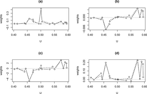
• In contrast to the univariable local linear regression where the weights are typically concentrated around the target point of estimation, the weights in Figure 1(a,c) are influenced by the covariate $X_{i2}$'s and the conditional variance function $r_{22}^c(\cdot )$ (Corollary 3.1), and may not be concentrated around the target point.

Figure 1. Example 4.1 of Section 4, comparison between the exact weight function (13(13) $\begin{array}{rl}& \sum _{i=1}^n(U_i-u_0{)}^q{W}_{\nu }^g(\frac{U_i-u_0}{h};X_{i2})={\delta }_{g,1}{\delta }_{\nu ,q};\\ & \sum _{i=1}^n{X}_{i2}(U_i-u_0{)}^q{W}_{\nu }^g(\frac{U_i-u_0}{h};X_{i2})={\delta }_{g,2}{\delta }_{\nu ,q}.\end{array}$(13) ) (solid lines) and its normalised asymptotic form (30(30) $\begin{array}{rl}{K}_{2,0}^{\ast }(\frac{U_i-u_0}{h};X_{i2}^c)& =\left(\frac{X_{i2}^c}{r_{22}^c\left(u_0\right)}\right)K\left(\frac{U_i-u_0}{h}\right),\\ K_{2,1}^{\ast }(\frac{U_i-u_0}{h};X_{i2}^c)& =\left(\frac{X_{i2}^c}{r_{22}^c\left(u_0\right)}\right)K_1^{\ast }\left(\frac{U_i-u_0}{h}\right)\\ & =\left(\frac{X_{i2}^c}{r_{22}^c\left(u_0\right)}\right)\left(\frac{U_i-u_0}{h{\mu }_2}\right)K\left(\frac{U_i-u_0}{h}\right)\\ & =\left(\frac{U_i-u_0}{h{\mu }_2}\right)K_{2,0}^{\ast }(\frac{U_i-u_0}{h};X_{i2}^c).\end{array}$(30) ) (dash lines) of ${\widehat{\text{β}}}_{2,0}$ with (a) q = 0 and (b) q = 1; of ${\widehat{\text{β}}}_{2,1}$ with (c) q = 0 and (d) q = 1.

Example 4.2

We set $X_{i2}$'s and $U_i$'s the same as those in Example 4.1, and further set $P\left(U_i\right)=U_i^2-1.5U$ to illustrate the reproducing property in Proposition 3.1 when d = 2 and p = 2. Again, let $u_0=0.5$ and h = 0.1, Figure 2(a) plots the points $(U_i,P(U_i\left)\right)$ as +'s, $i=39,\dots ,56$, and the weights $W_0^1\left(\right(U_i-u_0)/h;X_{i2})$ of g = 1 and $\nu =0$ reproducing $P\left(0.5\right)=-0.5$ (a solid black-square point) are plotted as circles with lines connecting them. There are a few negative weights since the weights are not necessarily nonnegative when p = 2 and d = 2. Figures 2(b,c) are similar to Figure 2(a) except for $\nu =1$ and 2 respectively; i.e. the + points $(U_i,P^{\left(\nu \right)}(U_i\left)\right)$'s and the weights $W_{\nu }^1\left(\right(U_i-u_0)/h;X_{i2})$ reproducing $P^{\left(\nu \right)}\left(0.5\right)$ ($P^{\mathrm{\prime }}\left(0.5\right)=-0.5$ and $P^{\mathrm{\prime \prime }}\left(0.5\right)=0$, solid black-square points) are shown. The variation of weights increases as ν increases, as shown by the scale of the y-axis.

Figure 2. Example 4.2 of Section 4. (a)–(c) for g = 1 and $\nu =$0, 1, 2, respectively: the +'s points are $(U_i,P^{\left(\nu \right)}(U_i\left)\right)$, $i=39,\dots ,56$, and the weights $W_{\nu }^1\left(\right(U_i-u_0)/h;X_{i2})$ reproducing $P^{\left(\nu \right)}\left(0.5\right)$ (a solid black-square point) are plotted as circles with lines. (d)-(f) for g = 2 and $\nu =$0, 1, 2, respectively: The + points $(U_i,\frac{{\mathrm{\partial }}^{\nu }}{\mathrm{\partial }{u}^{\nu }}Q(U_i,X_{i2}\left)\right)$'s and the weights $W_{\nu }^2\left(\right(U_i-u_0)/h;X_{i2})$ that reproduces $\frac{\mathrm{\partial }}{\mathrm{\partial }{x}_2}\left(\frac{{\mathrm{\partial }}^{\nu }}{\mathrm{\partial }{u}^{\nu }}Q\right(u,x_2\left){|}_{u=0.5}\right)$ (a solid black-square point) are shown.

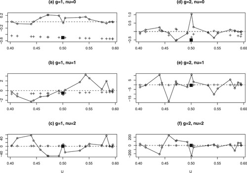
Analogous illustration is given in Figures 2(d–f) for g = 2 and $Q(U_i,X_{i2})=X_{i2}P\left(U_i\right)$. The + points $(U_i,\frac{{\mathrm{\partial }}^{\nu }}{\mathrm{\partial }{u}^{\nu }}Q(U_i,X_{i2}\left)\right)$'s and the weights $W_{\nu }^2\left(\right(U_i-u_0)/h;X_{i2})$ that reproduces $\frac{\mathrm{\partial }}{\mathrm{\partial }{x}_2}\left(\frac{{\mathrm{\partial }}^{\nu }}{\mathrm{\partial }{u}^{\nu }}Q\right(u,x_2\left){|}_{u=0.5}\right)=P^{\left(\nu \right)}\left(0.5\right)$ (a solid black-square point) are shown. Again, the variation of weights increases as ν increases, as shown by the scale of the y-axis. The difference of weights between g = 1 and 2 are visually obvious when comparing Figure 2(a–c,d–f).

Acknowledgments

We thank the Editor, an Associate Editor, and two referees for constructive suggestions and insightful comments.

Disclosure statement

No potential conflict of interest was reported by the author(s).

Additional information

Funding

C-Y Wu and L-H Huang were partially supported by the Ministry of Science and Technology, Taiwan, under Grants 107-2118-M-007-002-MY2, 105-2118-M-007-006-MY2 and 103-2118-M-007-001-MY2.

Appendix

Conditions A

The following assumptions are taken from Zhang and Lee (2000).

(A1)	$E{X}_j^{2s}<\mathrm{\infty }$ for some $s>2,j=2,\dots ,d$.
(A2)	Let $a_g^{\left(l\right)}$ denote the lth derivative of $a_g(\cdot )$; $a_g^{(p+1)}(\cdot )$ is continuous in a neighbourhood of $u_0$ for $g=1,\dots ,d$. Further, assume $a_g^{(p+1)}\left(u_0\right)\ne 0$, for $g=1,\dots ,d$.
(A3)	The functions $r_{\mathrm{jk}}(\cdot )$, $j,k=1,\dots ,d$ and ${\sigma }^2(\cdot )$ have bounded second derivatives in a neighbourhood of $u_0$.
(A4)	The marginal density $f_U\left(u\right)$ of U has a continuous second derivative in some neighbourhood of $u_0$ and $f_U\left(u_0\right)\ne 0$.
(A5)	The kernel function $K(\cdot )$ is a symmetric density function with compact support.

Proof

Proof of (22(22) $\begin{array}{rl}& \sum _{i=1}^n(U_i-u_0{)}^q{W}_{\nu }^g(\frac{U_i-u_0}{h};{\mathbf{x}}_{\left(i\right)}^T)={\delta }_{g,1}{\delta }_{\nu ,q},\\ & \sum _{i=1}^n{X}_{\mathrm{ik}}(U_i-u_0{)}^q{W}_{\nu }^g(\frac{U_i-u_0}{h};{\mathbf{x}}_{\left(i\right)}^T)={\delta }_{g,k}{\delta }_{\nu ,q}.\end{array}$(22) ) and Proposition 3.1

From (21(21) $W_{\nu }^g(\frac{U_i-u_0}{h};{\mathbf{x}}_{\left(i\right)}^T)={\zeta }_{g,\nu +1}^T{S}_n^{-1}({\tilde{\mathbf{x}}}_{\left(i\right)}\otimes {\mathbf{u}}_{i0})K_h(U_i-u_0)$(21) ), the LHS of the first equation in (22(22) $\begin{array}{rl}& \sum _{i=1}^n(U_i-u_0{)}^q{W}_{\nu }^g(\frac{U_i-u_0}{h};{\mathbf{x}}_{\left(i\right)}^T)={\delta }_{g,1}{\delta }_{\nu ,q},\\ & \sum _{i=1}^n{X}_{\mathrm{ik}}(U_i-u_0{)}^q{W}_{\nu }^g(\frac{U_i-u_0}{h};{\mathbf{x}}_{\left(i\right)}^T)={\delta }_{g,k}{\delta }_{\nu ,q}.\end{array}$(22) ) is $\begin{array}{rl}& \sum _{i=1}^n(U_i-u_0{)}^q{W}_{\nu }^g(\frac{U_i-u_0}{h};{\mathbf{x}}_{\left(i\right)}^T)={\zeta }_{g,\nu +1}^T{S}_n^{-1}\sum _{i=1}^n(U_i-u_0{)}^q({\tilde{\mathbf{x}}}_{\left(i\right)}\otimes {\mathbf{u}}_{i0})K_h(U_i-u_0)\\ & ={\zeta }_{g,\nu +1}^T{S}_n^{-1}{S}_n{\zeta }_{1,q+1}={\delta }_{g,1}{\delta }_{\nu ,q}.\end{array}$Analogously, the LHS of the second equation in (22(22) $\begin{array}{rl}& \sum _{i=1}^n(U_i-u_0{)}^q{W}_{\nu }^g(\frac{U_i-u_0}{h};{\mathbf{x}}_{\left(i\right)}^T)={\delta }_{g,1}{\delta }_{\nu ,q},\\ & \sum _{i=1}^n{X}_{\mathrm{ik}}(U_i-u_0{)}^q{W}_{\nu }^g(\frac{U_i-u_0}{h};{\mathbf{x}}_{\left(i\right)}^T)={\delta }_{g,k}{\delta }_{\nu ,q}.\end{array}$(22) ) is $\begin{array}{rl}& \sum _{i=1}^n{X}_{\mathrm{ik}}(U_i-u_0{)}^q{W}_{\nu }^g(\frac{U_i-u_0}{h};{\mathbf{x}}_{\left(i\right)}^T)={\zeta }_{g,\nu +1}^T{S}_n^{-1}\sum _{i=1}^n{X}_{\mathrm{ik}}(U_i-u_0{)}^q({\tilde{\mathbf{x}}}_{\left(i\right)}\otimes {\mathbf{u}}_{i0})K_h(U_i-u_0)\\ & ={\zeta }_{g,\nu +1}^T{S}_n^{-1}{S}_n{\zeta }_{k,q+1}={\delta }_{g,k}{\delta }_{\nu ,q}.\end{array}$Hence (22(22) $\begin{array}{rl}& \sum _{i=1}^n(U_i-u_0{)}^q{W}_{\nu }^g(\frac{U_i-u_0}{h};{\mathbf{x}}_{\left(i\right)}^T)={\delta }_{g,1}{\delta }_{\nu ,q},\\ & \sum _{i=1}^n{X}_{\mathrm{ik}}(U_i-u_0{)}^q{W}_{\nu }^g(\frac{U_i-u_0}{h};{\mathbf{x}}_{\left(i\right)}^T)={\delta }_{g,k}{\delta }_{\nu ,q}.\end{array}$(22) ) is obtained. Then we show the results of Proposition 3.1. For (23(23) $\nu !\sum _{i=1}^{n}P\left(U_i\right)W_{\nu }^g(\frac{U_i-u_0}{h};{\mathbf{x}}_{\left(i\right)}^T)={\delta }_{g,1}\left(\frac{d^{\nu }}{d{u}^{\nu }}P\right(u\left){|}_{u=u_0}\right);$(23) ), since $P(\cdot )$ is a polynomial of degree $\le p$, $P\left(U_i\right)=P\left(u_0\right)+P^{\mathrm{\prime }}\left(u_0\right)(U_i-u_0)+\cdots +\frac{P^{\left(p\right)}\left(u_0\right)}{p!}(U_i-u_0{)}^p.$Plugging this polynomial into the LHS of (23(23) $\nu !\sum _{i=1}^{n}P\left(U_i\right)W_{\nu }^g(\frac{U_i-u_0}{h};{\mathbf{x}}_{\left(i\right)}^T)={\delta }_{g,1}\left(\frac{d^{\nu }}{d{u}^{\nu }}P\right(u\left){|}_{u=u_0}\right);$(23) ), the RHS of (23(23) $\nu !\sum _{i=1}^{n}P\left(U_i\right)W_{\nu }^g(\frac{U_i-u_0}{h};{\mathbf{x}}_{\left(i\right)}^T)={\delta }_{g,1}\left(\frac{d^{\nu }}{d{u}^{\nu }}P\right(u\left){|}_{u=u_0}\right);$(23) ) is obtained based on the first equation in (22(22) $\begin{array}{rl}& \sum _{i=1}^n(U_i-u_0{)}^q{W}_{\nu }^g(\frac{U_i-u_0}{h};{\mathbf{x}}_{\left(i\right)}^T)={\delta }_{g,1}{\delta }_{\nu ,q},\\ & \sum _{i=1}^n{X}_{\mathrm{ik}}(U_i-u_0{)}^q{W}_{\nu }^g(\frac{U_i-u_0}{h};{\mathbf{x}}_{\left(i\right)}^T)={\delta }_{g,k}{\delta }_{\nu ,q}.\end{array}$(22) ). Since $Q(\cdot ,x_k)=x_{k}P(\cdot )$, analogous arguments can be derived for (24(24) $\nu !\sum _{i=1}^{n}Q(U_i;X_{\mathrm{ik}})W_{\nu }^g(\frac{U_i-u_0}{h};{\mathbf{x}}_{\left(i\right)}^T)={\delta }_{g,k}\frac{\mathrm{\partial }}{\mathrm{\partial }{x}_k}\left(\frac{{\mathrm{\partial }}^{\nu }}{\mathrm{\partial }{u}^{\nu }}Q\right(u,x_k\left){|}_{u=u_0}\right).$(24) ).

Proof

Proof of Theorem 3.2

From (14(14) $S_n^{-1}=\frac{1}{n{f}_U\left(u_0\right)}\left(\right[{\mathrm{\Omega }}_2\left(u_0\right){]}^{-1}\otimes {\mathcal{H}}_1^{-1}{\mathcal{S}}_1^{-1}{\mathcal{H}}_1^{-1})(1+O_p\left(\frac{\log n}{\sqrt{nh}}\right)),$(14) ), the matrix $S_n^{-1}$ for general d and p has an asymptotic form Zhang and Lee (2000, equation (5.2)) $S_n^{-1}=\frac{1}{n{f}_U\left(u_0\right)}\left(\right[{\mathrm{\Omega }}_d\left(u_0\right){]}^{-1}\otimes {\mathcal{H}}_p^{-1}{\mathcal{S}}_p^{-1}{\mathcal{H}}_p^{-1})(1+O_p\left(\frac{\log n}{\sqrt{nh}}\right)).$Then based on (3(3) $\widehat{\text{β}}\left(u_0\right)=({\mathbf{X}}_{u_0}^T{\mathbf{W}}_{u_0}{\mathbf{X}}_{u_0}{)}^{-1}{\mathbf{X}}_{u_0}^T{\mathbf{W}}_{u_0}\mathbf{y}.$(3) ), $\widehat{\text{β}}\left(u_0\right)=\sum _{i=1}^n\frac{1}{\mathrm{nh}{f}_U\left(u_0\right)}\left(\right[{\mathrm{\Omega }}_d\left(u_0\right){]}^{-1}\otimes {\mathcal{H}}_p^{-1}{\mathcal{S}}_p^{-1}{\mathcal{H}}_p^{-1})({\tilde{\mathbf{x}}}_{\left(i\right)}\otimes {\mathbf{u}}_i)K\left(\frac{U_i-u_0}{h}\right)Y_i\times (1+o_p(1\left)\right).$By properties of Kronecker product, the equivalent kernel corresponding to ${\widehat{\text{β}}}_{g,\nu }\left(u_0\right)={\zeta }_{g,\nu +1}^T\widehat{\text{β}}\left(u_0\right)$ (${\zeta }_{g,\nu +1}$ is derived as follows: $\begin{array}{rl}{\widehat{\text{β}}}_{g,\nu }\left(u_0\right)& =\sum _{i=1}^n\frac{1}{n{h}^{1+\nu }{f}_U\left(u_0\right)}\left(e_{d,g}^T\right[{\mathrm{\Omega }}_d\left(u_0\right){]}^{-1}{\tilde{\mathbf{x}}}_{\left(i\right)})\otimes \left(e_{p+1,\nu +1}^T{\mathcal{S}}_p^{-1}{\mathcal{H}}_p^{-1}{\mathbf{u}}_{i}K\left(\frac{U_i-u_0}{h}\right)\right)Y_i\\ & \times (1+o_p(1\left)\right)\\ & =\sum _{i=1}^n\frac{1}{n{h}^{1+\nu }{f}_U\left(u_0\right)}\left(e_{d,g}^T\right[{\mathrm{\Omega }}_d\left(u_0\right){]}^{-1}{\tilde{\mathbf{x}}}_{\left(i\right)}{K}_{\nu }^{\ast }\left(\frac{U_i-u_0}{h}\right))Y_i(1+o_p(1\left)\right).\end{array}$To show the moment property (27(27) $\begin{array}{r}\int t^q(\int \cdots \int K_{1,\nu }^{\ast }(t;x_2,\dots ,x_d\left)f\right(x_2,\dots ,x_d|u_0)\mathrm{d}{x}_2\cdots \mathrm{d}{x}_d)\mathrm{d}t={\delta }_{g,1}{\delta }_{\nu ,q},\\ \int t^q(\int \cdots \int x_k{K}_{g,\nu }^{\ast }(t;x_2,\dots ,x_d\left)f\right(x_2,\dots ,x_d|u_0)\mathrm{d}{x}_2\cdots \mathrm{d}{x}_d)\mathrm{d}t={\delta }_{g,k}{\delta }_{\nu ,q},\end{array}$(27) ), again by properties of Kronecker product, for $k=1,\dots ,d$, $\begin{array}{rl}& \int (\int \cdots \int {\zeta }_{g,\nu +1}^T({\mathrm{\Omega }}_d\left(u_0\right)\otimes {\mathcal{S}}_p{)}^{-1}(\left[\begin{array}{c}{x}_k\\ ⋮\\ x_d{x}_k\end{array}\right]\otimes \left[\begin{array}{c}{t}^q\\ ⋮\\ t^{p+q}\end{array}\right])K\left(t\right)f(x_2,\dots ,x_d|u_0)d{x}_2\cdots d{x}_d)\mathrm{dt}\\ & =\int {\zeta }_{g,\nu +1}^T\left({\mathrm{\Omega }}_d\right(u_0)\otimes {\mathcal{S}}_p{)}^{-1}(\left[\begin{array}{c}{r}_{1k}\left(u_0\right)\\ ⋮\\ r_{\mathrm{dk}}\left(u_0\right)\end{array}\right]\otimes \left[\begin{array}{c}{t}^q\\ ⋮\\ t^{p+q}\end{array}\right])K(t)\mathrm{d}t\\ & ={\zeta }_{g,\nu +1}^T\left({\mathrm{\Omega }}_d\right(u_0)\otimes {\mathcal{S}}_p{)}^{-1}[\left({\mathrm{\Omega }}_d\right(u_0\left)e_{d,k}\right)\otimes \left({\mathcal{S}}_p{e}_{p+1,q+1}\right)]\\ & ={\zeta }_{g,\nu +1}^T\left({\mathrm{\Omega }}_d\right(u_0)\otimes {\mathcal{S}}_p{)}^{-1}({\mathrm{\Omega }}_d\left(u_0\right)\otimes {\mathcal{S}}_p){\zeta }_{k,q+1}={\delta }_{g,k}{\delta }_{\nu ,q}.\end{array}$

References

- Chiang, C.-T., Rice, J.A., and Wu, C.O. (2001), ‘Smoothing Spline Estimation for Varying Coefficient Models with Repeatedly Measured Dependent Variables’, Journal of the American Statistical Association, 96, 605–619.
- Fan, J., and Gijbels, I. (1996), Local Polynomial Modelling and Its Applications, London: Chapman & Hall.
- Fan, J., and Zhang, W. (1999), ‘Statistical Estimation in Varying Coefficient Models’, Annals of Statistics, 27, 1491–1518.
- Fan, J., and Zhang, W. (2008), ‘Statistical Methods with Varying Coefficient Models’, Statistics and its Interface, 1, 179–195.
- Gasser, T., Müller, H.-G., and Mammitzsch, V. (1985), ‘Kernels for Nonparametric Curve Estimation’, Journal of the Royal Statistical Society: Series B Statistical Methodology, 47, 238–252.
- Hastie, T.J., and Tibshirani, R.J. (1993), ‘Varying-Coefficient Models’, Journal of the Royal Statistical Society: Series B Statistical Methodology, 55, 757–796.
- Park, B.U., Mammen, E., Lee, Y.K., and Lee, E.R. (2015), ‘Varying Coefficient Regression Models: a Review and New Developments’, International Statistical Review, 83, 36–64.
- Petersen, A., and Müller, H.-G. (2019), ‘Fréchet Regression for Random Objects with Euclidean Predictors’, Annals of Statistics, 47, 691–719.
- Ruppert, D., Wand, M.P., and Carroll, R.J. (2003), Semiparametric Regression, London: Cambridge University Press.
- Tsybakov, A.B. (2009), Introduction to Nonparametric Estimation, New York: Springer-Verlag.
- Zhang, W., and Lee, S.Y. (2000), ‘Variable Bandwidth Selection in Varying-Coefficient Models’, Journal of Multivariate Analysis, 74, 116–134.