Robust oracle estimation and uncertainty quantification for possibly sparse quantiles

Abstract

A general many quantiles + noise model is studied in the robust formulation (allowing non-normal, non-independent observations), where the identifiability requirement for the noise is formulated in terms of quantiles rather than the traditional zero expectation assumption. We propose a penalisation method based on the quantile loss function with appropriately chosen penalty function making inference on possibly sparse high-dimensional quantile vector. We apply a local approach to address the optimality by comparing procedures to the oracle sparsity structure. We establish that the proposed procedure mimics the oracle in the problems of estimation and uncertainty quantification (under the so-called EBR condition). Adaptive minimax results over sparsity scale follow from our local results.

KEYWORDS:

• Estimation
• oracle rate
• oracle sparsity structure
• quantile loss
• uncertainty quantification

1. Introduction

Since the emergence of statistical science, the classical ‘signal+noise’ paradigm for observed data is the main testbed in theoretical statistics for a vast number of methods and techniques for various inference problems and in various optimality frameworks. Many other practically important situations can be reduced to or approximated by the ‘signal+noise’ setting, capturing the statistical essence of the original (typically, more complex) model and preserving its main features in a pure form. There is a huge literature on ‘signal+noise’ setting with big variety of combinations of the main ingredients in the study. We mention the following ingredients: assumptions on the observation model (moment conditions, independence, normality, etc.); applied methodology (LSE, penalisation, shrinkage, thresholding, (empirical) Bayesian approach, projection, FDR method); studied inference problem (estimation, detection, model selection, testing, posterior contraction, uncertainty quantification, structure recovery); structural assumptions (smoothness, sparsity, clustering, shape constraints, such as monotonicity, unimodality and convexity, loss functions (expectations of powers of ${\ell }_2$-norm, ${\ell }_q$-norm; Hamming loss, etc.); optimality framework and pursued criteria (minimax rate, oracle rate, control of FDR, FNR, expectation of the loss function, exponential bounds for the large deviations of the loss functions, etc.). A small sample of relevant literature includes (Donoho, Johnstone, Hoch, and Stern 1992; Donoho and Johnstone 1994; Benjamini and Hochberg 1995; Birgé and Massart 2001; Johnstone and Silverman 2004; Baraud 2004; Abramovich, Benjamini, Donoho, and Johnstone 2006; Efron 2008; Babenko and Belitser 2010; Belloni, Chernozhukov, and Wang 2011; Castillo and van der Vaart 2012; Martin and Walker 2014; Johnstone 2017; Belitser 2017; Bellec 2018; Butucea, Ndaoud, Stepanova, and Tsybakov 2018; Belitser and Nurushev 2020).

Suppose we observe $X=(X_1,\dots ,X_n)\sim {\mathbb{P}}_{\theta }^n$, where $\theta =({\theta }_1,\dots ,{\theta }_n)\in {\mathbb{R}}^n$ is the parameter of interest. We shall suppress n from the notation to simply write ${\mathbb{P}}_{\theta }$ for ${\mathbb{P}}_{\theta }^n$. A natural example is given by $X_i\stackrel{\mathrm{ind}}{\sim }\mathrm{N}({\theta }_i,1)$, $i=1,\dots ,n$, but this specific distributional assumption on the data generating process will not be imposed. The main modelling assumption in this note is that, for some fixed level $\tau \in (0,1)$, $\mathbb{P}(X_i-{\theta }_i\le 0)=\tau ,i=1,\dots ,n.$In other words, we deal with the setting many quantiles + noise, as ${\theta }_i$'s are the τ-quantiles of the observed $X_i$'s and the goal is to make an inference on the high-dimensional parameter θ. One can study and make inference on several quantiles simultaneously across different levels $\tau \in (0,1)$. While the mean is a commonly used measure of centrality, it is heavily influenced by outliers or extreme values in the dataset. In contrast, quantiles are robust to outliers and provide information about the spread of the data as well as the location of the central values, cf., Zou and Yuan (2008), Jiang, Wang, and Bondell (2013) and Jiang, Bondell, and Wang (2014). The setting ‘many quantiles + noise’ with sparse quantile vectors arises in statistical and machine learning applications where the goal is to estimate a large number of quantiles for a high-dimensional dataset. The number of quantiles to be estimated can be very large, while the data may be sparse, meaning that only a small fraction of the entries in the data are non-zero. In such applications, quantiles may be a more sensible object of study, especially when the distribution is skewed or contains outliers. In this setting, the interest of study focuses on the effect of the parameter values on the tails of a distribution of observations, in addition to, or instead of, the centre. For example, in finance, quantiles such as the value at risk (the value at risk in finance has the meaning of quantile) or expected shortfall are commonly used to estimate the potential losses of a portfolio of investments, rather than relying solely on the mean return. Estimating a large number of quantiles is important for risk management and portfolio optimisation, as it provides a more complete picture of the potential losses or gains of a portfolio. In genomics, estimating many quantiles can help identify genes or markers that are associated with disease. In image processing, estimating quantiles can help identify regions of interest or anomalies in images. Quantiles as objects of interest occur in diverse areas, including economics, biology, meteorology; cf. Santosa and Symes (1986), Abrevaya (2002), Koenker (2005), Belloni and Chernozhukov (2011), Hulmán et al. (2015), Gabriela Ciuperca (2018) and Belloni, Chernozhukov, and Kato (2019).

Besides quantile formulation, the next distinctive feature of our study is the robust formulation in the sense that we do not assume any particular form of the distribution of the observed data. Only a mild condition (Condition C1) is imposed. The observations do not need to be normal and, in fact no specific distribution is assumed, the distribution of the ‘noise’ terms $X_i-{\theta }_i$, $i=1,\dots ,n$, may depend on θ and do not even have to be independent. This makes the applicability scope of our results rather broad.

The third aspect of our study is the local approach. It is in general impossible to make sensible inference on a high-dimensional parameter without any additional structure, either in terms of assumptions on parameter, or on the observation model, or both. In this paper, we are concerned with sparsity structure, various version of which have been predominantly studied in the literature recently. Sparsity structure means that a relative majority of the parameter entries are all equal to some fixed value (typically zero). In the local approach, we address optimality by comparing procedures to the oracle sparsity structure (think of an ‘oracle observer’ that knows the best sparsity pattern of the actual θ). When applying the local approach, the idea is not to rely on sparsity as such, but rather extract all the sparsity structure present in the data, and utilise it in the aimed inference problems. The claim that a procedure performs optimally in the local sense means that it attains the oracle quality, i.e. mimics the best sparsity structure pertinent to the true parameter, whichever it is. The local result imply minimax optimality over all scales (including the traditional sparsity class ${\ell }_0[s]$) that satisfy a certain condition.

The final feature of our study concerns the problem of uncertainty quantification. In recent years, focus in nonparametric statistics has shifted from point estimation to uncertainty quantification, a more challenging problem, much less results on this topic are available in the literature; cf. Szabó, van der Vaart, and van Zanten (2015), Belitser (2017), van der Pas, Szabó, and van der Vaart (2017) and Belitser and Nurushev (2020). Certain negative results (cf. Li 1989; Baraud 2004; Belitser and Nurushev 2019 and the references therein) show that in general a confidence set cannot simultaneously have coverage and the optimal size uniformly over all parameter values. This makes the construction of the so-called ‘honest’ confidence sets impossible, and a strategy recently pursued in the literature is to discard a set of ‘deceptive parameters’ to ensure coverage at the remaining parameter values, while maintaining the optimal size uniformly over the whole set. In an increasing order of generality, removing deceptive parameters is expressed by imposing the conditions of self-similarity, polished tail and excessive bias restriction (EBR), see Szabó et al. (2015), Belitser (2017), van der Pas et al. (2017) and Belitser and Nurushev (2020). All the above papers deal with ${\ell }_2$-loss framework for Gaussian observations in ‘many means + noise’ setting (a more general case is considered in Belitser and Nurushev 2020).

In this paper, we work with a new setting ‘many quantiles + general noise’, and use the quantile loss rather than the traditional ${\ell }_2$-loss. The quantile loss function has certain properties of usual loss functions, but it is not symmetric, the peculiarity essentially characterising the notion of quantile. We propose and exploit a new version of EBR condition expressed in terms of quantile loss. To the best of our knowledge, there are no results on uncertainty quantification neither for the quantile loss function, nor for the ${\ell }_1$-loss, also neither in local, nor global (minimax) formulation in this general robust setting. In this respect, our study presents the first step in this direction.

We finally summarise the main contributions of this paper.

• For our new (robust) setting ‘many quantiles + general noise’ we propose a penalisation procedure for selecting the sparsity pattern, based on the quantile loss (as counterpart of the ${\ell }_2$-loss) and the corresponding penalty term.

• The estimated sparsity pattern is next used for the construction of an estimator of θ and a confidence set for θ, again in terms of the quantile loss function.

• Two theorems establish the local (oracle) optimality of the estimator and confidence set (under the EBR condition), respectively.

• We provide an elegant and relatively short proofs of the main results; compare with the relatively laborious proofs of related results in Szabó et al. (2015), Belitser (2017), van der Pas et al. (2017) and Belitser and Nurushev (2020).

• The obtained results are robust and local in the sense explained above.

• The obtained local results imply adaptive minimax optimality for scales of classes that satisfy certain relation (in particular, for the traditional sparsity scale).

Organisation of the rest of the paper is as follows. In Section 2, we give a robust formulation of the observation model in the ‘many quantiles + general noise’ setting, and introduce some notations and preliminaries. In Section 3, we present the main results of the paper and discuss their consequences for the optimality in the minimax sense for the traditional sparsity scale. Section 4 contains a small simulation study. The proofs of the theorems are provided in Section 5.

2. Robust model formulation and preliminaries

We can formally rewrite the model stated in the introduction in the familiar ‘signal+noise’ form: (1) $X_i={\theta }_i+{\xi }_i,{\mathbb{P}}_{\theta }({\xi }_i\le 0)=\tau ,i\in [n]=\{1,\dots ,n\}.$(1) where ${\xi }_i=X_i-{\theta }_i$ can be thought of as ‘noise’. Note that all the quantities depend of course on τ. Precisely, for $\tau \in (0,1)$, in the model (1(1) $X_i={\theta }_i+{\xi }_i,{\mathbb{P}}_{\theta }({\xi }_i\le 0)=\tau ,i\in [n]=\{1,\dots ,n\}.$(1) ) we have $\theta =\theta (\tau )$, $\xi =\xi (\tau )$ with ${\mathbb{P}}_{\theta }({\xi }_i(\tau )\le 0)=\tau$, $i=1,\dots ,n$. Not to overload the notation, we suppress the dependence on τ in the sequel. As we mentioned in the Introduction, we study robust setting in the sense that we do not assume any particular distribution of $\xi =({\xi }_1,\dots ,{\xi }_n)$. In fact, the ${\xi }_i$'s do not have to be identically distributed, their distribution may depend on θ and they do not even have to be independent.

Introduce the following asymmetric absolute deviation function: $\rho (x)={\rho }_{\tau }(x)={\rho }_{\tau ,m}(x)=\sum _{i=1}^m{x}_i(\tau -1\{x_i\le 0\}),x\in {\mathbb{R}}^m,m\in \mathbb{N},$which we will also call quantile loss function, $1\{E\}$ denotes the indicator of event E.

Slightly abusing notation, we use the same notation $\rho (x)$ for any $m\in \mathbb{N}$, for example, most of the time it will be either m = n or m = 1, depending on the dimensionality of the argument of the function. This will always be clear from the context. Often, we will suppress the dependence of ρ on a fixed $\tau \in (0,1)$, unless emphasising this dependence where it is relevant.

Remark 2.1

The origin of the quantile loss function ${\rho }_{\tau }(x)$, $x\in \mathbb{R}$, is well explained in the book (Koenker 2005). The function ${\rho }_{\tau }(x)$ characterises the τ-quantile of a random variable Z in the sense that the τ-quantile ${\theta }_{\tau }$ of Z is known to minimise the criterion function $\mathbb{E}{\rho }_{\tau }(Z-\vartheta )$ with respect to ϑ, i.e. $\arg \underset{\vartheta \in \mathbb{R}}{min}\mathbb{E}{\rho }_{\tau }(Z-\vartheta )={\theta }_{\tau }$. Basically, this function plays the same role for characterising the quantiles as the quadratic function in characterising the expectation of a random variable.

The quantile loss function ρ can be related to the ${\ell }_1$-criterion $|x|=\sum _{i=1}^m|x_i|$, $x=(x_1,\dots ,x_m)\in {\mathbb{R}}^m$: for any $\tau \in (0,1)$, (2) $(1-c_{\tau })|x|\le {\rho }_{\tau }(x)\le c_{\tau }|x|,\mathrm{with}{c}_{\tau }=max\{\tau ,1-\tau \}.$(2) In particular, it follows that ${\rho }_{1/2}(x)=|x|/2$. Another useful property of the quantile loss function ρ to be used later on is that, for any $x\in {\mathbb{R}}^m$, (3) ${\rho }_{\tau }(-x)\le C_{\tau }{\rho }_{\tau }(x),\mathrm{with}{C}_{\tau }=max\{\frac{1-\tau }{\tau },\frac{\tau }{1-\tau }\}=\frac{c_{\tau }}{1-c_{\tau }}.$(3)

Remark 2.2

The above quantile loss function evaluated at the difference $\rho (x-y)$, $x,y\in {\mathbb{R}}^m$, possesses all the properties of a metric $d(x,y)$ except for the symmetry. In particular, $\rho (0)=0$ (zero at zero); if $x\ne y$, $\rho (x-y)>0$ (positivity); and finally the triangle inequality holds (4) $\rho (x+y)\le \rho (x)+\rho (y),x,y\in {\mathbb{R}}^m.$(4)

Since we have as many parameters as observations, it is typically impossible to make inference on θ even in a weak sense unless the data possesses some structure. Here, we work with the structural assumption that θ is (possibly) a sparse vector. Specifically, we assume that $\theta \in L_I$, where  $I\subseteq [n]=\{1,\dots ,n\}$ and $L_I=\{x\in {\mathbb{R}}^n:x_i=0,i\in I^c\}$, where $I^c=[n]\setminus I$. The structure studied here is the unknown ‘true’ sparsity pattern $I_0=I_0(\theta )\subseteq [n]$, that is, $\theta \in L_{I_0}$ and $I_0$ is the ‘minimal’ sparsity structure in the sense that $I_0=\arg \underset{I\subseteq [n]:L_I\ni \theta }{min}\sum _{i\in I}i$.

Introduce some further notation: let $\mathcal{I}$ denote the family of all subsets of $[n]$; for $x\in {\mathbb{R}}^n$, denote its ${\ell }_1$-norm by $|x|=\sum _{i=1}^n|x_i|$; $|S|$ denote the cardinality of a set S. Further let us introduce the so-called ‘quantile projection’ ${\mathrm{P}}_I$ onto $L_I$ (called just projection in what follows), with respect to the quantile loss function $\rho (x-y)$. For $x\in {\mathbb{R}}^n$, define ${\mathrm{P}}_{I}x$ as follows: $\underset{y\in L_I}{inf}\rho (x-y)=\rho (x-{\mathrm{P}}_{I}x).$In view of the properties of the quantile loss function ρ given by Remark 2.2, the projection ${\mathrm{P}}_I$ is readily found as the following linear operator: ${\mathrm{P}}_{I}x=(x_{i}1\{i\in I\},i=1,\dots ,n)\in {\mathbb{R}}^n.$We will use later a certain monotonicity property of the quantile projection operator. (5) $\mathrm{If}{I}_1\subseteq I_2,\mathrm{then}\rho ({\mathrm{P}}_{I_1}x)\le \rho ({\mathrm{P}}_{I_2}x),x\in {\mathbb{R}}^n.$(5) For $s\ge 0$ and $I\in \mathcal{I}$, denote (with the convention $0\log (a/0)=0$ for a>0) $\lambda (s)=s\log (en/s),p(I)={(|I|\lambda (|I|))}^{1/2}=|I|{[\log (en/|I|)]}^{1/2}.$We have that $\lambda (s)\ge s$ for $s\in [0,n]$, and besides, since $\lambda (s)$ is increasing in $s\in (0,n]$, $\lambda (s)\ge 1+\log (n)$ for all $s\in [n]$. The function $p(I)$ has a meaning of complexity of structure I.

The following relation will be used later: for any $\nu >1$, (6) $\sum _{I\in \mathcal{I}}{e}^{-\nu \lambda (|I|)}=1+\sum _{s\in [n]}\sum _{I:|I|=s}{e}^{-\nu \lambda (s)}\le 1+\sum _{s\in [n]}{e}^{-(\nu -1)s}\le C_{\nu },$(6) with $C_{\nu }=1+(e^{\nu -1}-1{)}^{-1}<\mathrm{\infty }$.

The following conditions on $\xi =X-\theta$ is assumed throughout.

Condition C1. For some $H_0,M_0>0$ and some positive function $\psi (u)$ monotonically increasing to infinity as $u\to \mathrm{\infty }$, and all $I\in \mathcal{I}$, $I\ne \varnothing$, all $M\ge 0$, (7) $\underset{\theta \in {\mathbb{R}}^n}{sup}{\mathbb{P}}_{\theta }(\rho ({\mathrm{P}}_I\xi )>Mp(I))\le H_0{e}^{-(\psi (M)-M_0)\lambda (|I|)}.$(7) Notice that Condition C1 is trivially fulfilled for $I=\varnothing$ with zero right-hand side. Let $\mathcal{P}=\mathcal{P}(H_0,M_0,\psi )$ stand for the family of distributions ${\mathbb{P}}_{\theta }$ satisfying Condition C1.

As $\lambda (s)\ge 1+\log (n)$ for all $s\in [n]$, the right-hand side of (7(7) $\underset{\theta \in {\mathbb{R}}^n}{sup}{\mathbb{P}}_{\theta }(\rho ({\mathrm{P}}_I\xi )>Mp(I))\le H_0{e}^{-(\psi (M)-M_0)\lambda (|I|)}.$(7) ) is further bounded by $H_0{e}^{-(\psi (M)-M_0)\lambda (1)}\le H_0{n}^{-(\psi (M)-M_0)}$, which we will use in the proof.

Remark 2.3

Condition C1 is mild, for instance, it holds for independent sub-gaussian ${\xi }_i$'s. Recall one of the equivalent definitions of sub-gaussianity (see Vershynin 2018): a random variable W is called σ- sub-gaussian for $\sigma >0$ if for some $c_0>0$ $\mathbb{E}{e}^{c_0{W}^2/{\sigma }^2}\le 2$. In our case, $\sigma =1$. For example, for ${\xi }_i\stackrel{\mathrm{ind}}{\sim }\mathrm{N}(0,1)$, $c_0=3/8$ (see Section 4). Recall that $\Vert x{\Vert }^2=\sum _{i=1}^n{x}_i^2$ denotes the usual squared ${\ell }_2$-norm of $x\in {\mathbb{R}}^n$. Now, since ${\mathrm{P}}_I\xi$ has at most $|I|$ non-zero entries, by (2(2) $(1-c_{\tau })|x|\le {\rho }_{\tau }(x)\le c_{\tau }|x|,\mathrm{with}{c}_{\tau }=max\{\tau ,1-\tau \}.$(2) ) and the Cauchy–Schwartz inequality we have $\rho ({\mathrm{P}}_I\xi )\le c_{\tau }|{\mathrm{P}}_I\xi |\le c_{\tau }|I{|}^{1/2}\Vert {\mathrm{P}}_I\xi \Vert$ (this also follows from the following inequality between two different ${\ell }_q$-norms: for $x\in {\mathbb{R}}^n$ and $0<q_1<q_2\le \mathrm{\infty }$, $\Vert x{\Vert }_{q_2}\le \Vert x{\Vert }_{q_1}\le n^{1/q_1-1/q_2}\Vert x{\Vert }_{q_2}$). Recall also that $\lambda (s)\ge s$, $s\in [0,n]$. Using these and the Markov inequality, we obtain that, for $H_0=1$, $\psi (M)=c_0{c}_{\tau }^{-2}{M}^2$ and $M_0=\log 2$, $\begin{array}{rl}\mathbb{P}(\rho ({\mathrm{P}}_I\xi )\ge Mp(I))& \le \mathbb{P}(c_{\tau }|I{|}^{1/2}\Vert {\mathrm{P}}_I\xi {\Vert }_2\ge Mp(I))\\ & =\mathbb{P}(\Vert {\mathrm{P}}_I\xi {\Vert }_2\ge \frac{M}{c_{\tau }}[\lambda (|I|){]}^{1/2})\\ & \le \mathbb{P}(c_0\Vert {\mathrm{P}}_I\xi {\Vert }_2^2\ge c_0{c}_{\tau }^{-2}{M}^2\lambda (|I|))\\ & \le e^{|I|\log 2-c_0{c}_{\tau }^{-2}{M}^2\lambda (|I|)}\le e^{-(\psi (M)-M_0)\lambda (|I|)}.\end{array}$One can extend the results to the case of the so-called sub-exponential errors, with adjusted complexity function $p(I)$; see Remark 3.3.

Remark 2.4

Condition C1 is clearly satisfied for bounded, arbitrarily dependent, ${\xi }_i$'s. This condition allows some interesting cases of dependent ${\xi }_i$'s. By arguing in the same way as in Belitser and Nurushev (2020), we can establish that Condition C1 holds also for ${\xi }_k$'s which follow an autoregressive model AR(1) with sub-gaussian white noise ${ϵ}_k$'s (for appropriately chosen model parameters): ${\xi }_k=\alpha {\xi }_{k-1}+{ϵ}_k,k\in [n];{\xi }_0=0,|\alpha |<1.$In Belitser and Nurushev (2020), the normal white noise was used in the above model AR(1), but this can easily be extended to the sub-gaussian case by adjusting the constants involved.

Remark 2.5

We can extend our setting by including also a parameter $\sigma >0$ by considering $\sigma {\xi }_i$ instead of just ${\xi }_i$ (and $(X_i-\theta )/\sigma$ instead of $X_i-\theta$) in (1(1) $X_i={\theta }_i+{\xi }_i,{\mathbb{P}}_{\theta }({\xi }_i\le 0)=\tau ,i\in [n]=\{1,\dots ,n\}.$(1) ) and in Condition C1. In that case, the parameter $\sigma >0$ is assumed to be known and fixed throughout. Together with n, it reflects the information amount in the model in the sense that $\sigma \to 0$ means the flux of information.

We propose a penalised projection estimator. For $\kappa >0$, define $\hat{I}=\hat{I}(X,\kappa )$ to be a minimiser of the criterion $C(I)=C(I,\kappa )=C(I,\kappa ,X)$: (8) $\begin{array}{rl}C(I)& =\rho (X-{\mathrm{P}}_{I}X)+\kappa p(I)=\rho ({\mathrm{P}}_{I^c}X)+\kappa p(I),\\ \underset{I\in \mathcal{I}}{min}C(I)& =C(\hat{I}).\end{array}$(8)

Remark 2.6

Since the proposed procedure $\hat{I}$ for selecting sparsity pattern is based on the non-symmetric quantile loss function ρ, the deviations from below and from above are treated differently. But the computation of the estimator $\hat{I}$ of the sparsity pattern is not difficult. Indeed, it can be reduced to the search over n options: with $b_k=\rho (X_k)\ge 0$, $k\in [n]$, $\begin{array}{rl}\underset{I\in \mathcal{I}}{min}C(I)& =\underset{I\in \mathcal{I}}{min}\{\rho ({\mathrm{P}}_{I^c}X)+\kappa p(I)\}=\underset{I\in \mathcal{I}}{min}\{\sum _{k\in I^c}\rho (X_k)+\kappa p(I)\}\\ & =\underset{i\in [n]}{min}\{\underset{I\in \mathcal{I}:|I|=i}{min}\sum _{k\in I^c}\rho (X_k)+\kappa i{\log }^{1/2}(\frac{en}{i})\}\\ & =\underset{i\in [n]}{min}\{\sum _{k=1}^{n-i}{b}_{(k)}+\kappa (i{\log }^{1/2}(\frac{en}{i})\}=\underset{i\in [n]}{min}\{B_i+\kappa (i{\log }^{1/2}(\frac{en}{i})\},\end{array}$where $b_{(1)}\le \cdots \le b_{(n)}$ is the ordered sequence of $b_k$'s and $B_i=\sum _{k=1}^{n-i}{b}_{(k)}$.

Now, using the estimated sparsity structure $\hat{I}$, define the estimator (9) $\hat{\theta }=\hat{\theta }(X,\kappa )={\mathrm{P}}_{\hat{I}}X.$(9) From the triangle inequality (4(4) $\rho (x+y)\le \rho (x)+\rho (y),x,y\in {\mathbb{R}}^m.$(4) ), it follows that $\rho (x-y)\ge \rho (x)-\rho (y)$. Using this, (3(3) ${\rho }_{\tau }(-x)\le C_{\tau }{\rho }_{\tau }(x),\mathrm{with}{C}_{\tau }=max\{\frac{1-\tau }{\tau },\frac{\tau }{1-\tau }\}=\frac{c_{\tau }}{1-c_{\tau }}.$(3) ) and the definition (8(8) $\begin{array}{rl}C(I)& =\rho (X-{\mathrm{P}}_{I}X)+\kappa p(I)=\rho ({\mathrm{P}}_{I^c}X)+\kappa p(I),\\ \underset{I\in \mathcal{I}}{min}C(I)& =C(\hat{I}).\end{array}$(8) ), we derive that, for any $I^{\prime }\in \mathcal{I}$, (10) $\begin{array}{rl}\kappa (p(\hat{I})-p(I^{\prime }))& \le \rho ({\mathrm{P}}_{I^{\prime c}}X)-\rho ({\mathrm{P}}_{{\hat{I}}^c}X)=\rho ({\mathrm{P}}_{\hat{I}\mathrm{\setminus }{I}^{\prime }}X)-\rho ({\mathrm{P}}_{I^{\prime }\mathrm{\setminus }\hat{I}}X)\\ & \le \rho ({\mathrm{P}}_{\hat{I}\mathrm{\setminus }{I}^{\prime }}\theta )+\rho ({\mathrm{P}}_{\hat{I}\mathrm{\setminus }{I}^{\prime }}\xi )-\rho ({\mathrm{P}}_{I^{\prime }\mathrm{\setminus }\hat{I}}\theta )+\rho ({\mathrm{P}}_{I^{\prime }\mathrm{\setminus }\hat{I}}(-\xi ))\\ & \le \rho ({\mathrm{P}}_{I^{\prime c}}\theta )-\rho ({\mathrm{P}}_{{\hat{I}}^c}\theta )+\rho ({\mathrm{P}}_{\hat{I}}\xi )+C_{\tau }\rho ({\mathrm{P}}_{I^{\prime }}\xi ).\end{array}$(10) For $\varkappa >0$, $\theta \in {\mathbb{R}}^n$ and $I\in \mathcal{I}$, introduce the quantity $r(\theta ,I)=r_{\varkappa }(\theta ,I)=\rho (\theta -{\mathrm{P}}_I\theta )+\varkappa p(I)=\rho ({\mathrm{P}}_{I^c}\theta )+\varkappa p(I),$which we call the quantile rate of the sparsity structure I. The oracle sparsity structure $I_o=I_o(\theta )=I_o(\theta ,\varkappa )$ is the one minimising $r_{\varkappa }(\theta ,I)$: (11) $\underset{I\in \mathcal{I}}{min}{r}_{\varkappa }(\theta ,I)=r_{\varkappa }(\theta ,I_o)=r_{\varkappa }(\theta )=r(\theta ).$(11) where its minimal value $r(\theta )$ is called the oracle quantile rate, or just oracle rate.

3. Main results

In this section, we give the main results. All the constants in the below assertions depend on the fixed constants $M_0,H_0$ and function ψ appearing in Condition C1, the constant κ appearing in the oracle structure definition (8(8) $\begin{array}{rl}C(I)& =\rho (X-{\mathrm{P}}_{I}X)+\kappa p(I)=\rho ({\mathrm{P}}_{I^c}X)+\kappa p(I),\\ \underset{I\in \mathcal{I}}{min}C(I)& =C(\hat{I}).\end{array}$(8) ), and the quantile level τ.

The next result concerns the estimation problem.

Theorem 3.1

Estimation

Let Condition C1 be fulfilled. Then for any $\varkappa >0$ and sufficiently large κ, there exist positive $M_1,H_1,m_1$ such that (12) ${\mathbb{P}}_{\theta }(\rho (\theta -\hat{\theta })\ge M_{1}r(\theta ))\le H_1{e}^{-m_1\lambda (1)}\le H_1{n}^{-m_1},\theta \in {\mathbb{R}}^n,$(12) where $\hat{\theta }$ is defined by (9(9) $\hat{\theta }=\hat{\theta }(X,\kappa )={\mathrm{P}}_{\hat{I}}X.$(9) ).

Next we address the new problem of uncertainty quantification (UQ) for the parameter θ. A confidence set is defined in terms of quantile loss function ρ as follows: (13) $B(\tilde{\theta },\tilde{r})=\{\theta \in {\mathbb{R}}^n:\rho (\theta -\tilde{\theta })\le \tilde{r}\},$(13) where the ‘ centre’ $\tilde{\theta }=\tilde{\theta }(X):{\mathbb{R}}^n\mapsto {\mathbb{R}}^n$ and ‘radius’ $\tilde{r}=\tilde{r}(X):{\mathbb{R}}^n\mapsto {\mathbb{R}}_{+}=[0,+\mathrm{\infty }]$ are measurable functions of the data X. The goal is to construct such a confidence set $B(\tilde{\theta },C\tilde{r})$ that for any ${\alpha }_1,{\alpha }_2\in (0,1]$ and some function $R(\theta )$, $R:{\mathbb{R}}^n\to {\mathbb{R}}_{+}$, there exist C, c>0 such that (14) $\underset{\theta \in {\mathrm{\Theta }}_{\mathrm{cov}}}{sup}{\mathbb{P}}_{\theta }(\theta \notin B(\tilde{\theta },C\tilde{r}))\le {\alpha }_1,\underset{\theta \in {\mathrm{\Theta }}_{\mathrm{size}}}{sup}{\mathbb{P}}_{\theta }(\tilde{r}\ge cR(\theta ))\le {\alpha }_2,$(14) for some ${\mathrm{\Theta }}_{\mathrm{cov}},{\mathrm{\Theta }}_{\mathrm{size}}\subseteq {\mathbb{R}}^n$. The function $R(\theta )$, called radial rate, is a benchmark for the effective radius of the confidence set $B(\tilde{\theta },C\tilde{r})$. The first expression in (14(14) $\underset{\theta \in {\mathrm{\Theta }}_{\mathrm{cov}}}{sup}{\mathbb{P}}_{\theta }(\theta \notin B(\tilde{\theta },C\tilde{r}))\le {\alpha }_1,\underset{\theta \in {\mathrm{\Theta }}_{\mathrm{size}}}{sup}{\mathbb{P}}_{\theta }(\tilde{r}\ge cR(\theta ))\le {\alpha }_2,$(14) ) is called coverage relation and the second size relation. It is desirable to find the smallest $r(\theta )$, the biggest ${\mathrm{\Theta }}_{\mathrm{cov}}$ and ${\mathrm{\Theta }}_{\mathrm{size}}$ such that (14(14) $\underset{\theta \in {\mathrm{\Theta }}_{\mathrm{cov}}}{sup}{\mathbb{P}}_{\theta }(\theta \notin B(\tilde{\theta },C\tilde{r}))\le {\alpha }_1,\underset{\theta \in {\mathrm{\Theta }}_{\mathrm{size}}}{sup}{\mathbb{P}}_{\theta }(\tilde{r}\ge cR(\theta ))\le {\alpha }_2,$(14) ) holds and $R(\theta )\asymp r({\mathrm{\Theta }}_{\mathrm{size}})$, where $r({\mathrm{\Theta }}_{\mathrm{size}})$ is the optimal rate in estimation problem for θ. In our local approach, we pursue even more ambitious goal $R(\theta )\asymp r(\theta )$, where $r(\theta )$ is the oracle rate from the (local) estimation problem.

Typically, the so-called deceptiveness issue arises for the UQ problem in that the confidence set of the optimal size and high coverage can only be constructed for non-deceptive parameters (in particular, ${\mathrm{\Theta }}_{\mathrm{cov}}$ cannot be the whole set ${\mathbb{R}}^n$). That is, coverage with an optimal sized radius is only possible if certain deceptive set of parameters is excluded from consideration, which is expressed by imposing some condition on the parameter. For example, the EBR (excessive bias restriction) condition in case of ${\ell }_2$-norm is proposed in Belitser and Nurushev (2019), Belitser (2017) and Belitser and Ghosal (2020). Here we need an EBR-like condition (we keep the same term EBR), but now in terms of the quantile loss function ρ.

Condition EBR. We say that parameter $\theta \in {\mathbb{R}}^n$ satisfies the excessive bias restriction (EBR) condition with structural parameter $t\ge 0$ if $\theta \in {\mathrm{\Theta }}_{\mathrm{eb}}(t)={\mathrm{\Theta }}_{\mathrm{eb}}(t,\varkappa )$ where (15) ${\mathrm{\Theta }}_{\mathrm{eb}}(t)=\{\theta \in {\mathbb{R}}^n:\frac{\rho (\theta -{\mathrm{P}}_{I_o}\theta )}{p(I_o)}\le t\},$(15) the oracle structure $I_o=I_o(\theta )$ is defined by (11(11) $\underset{I\in \mathcal{I}}{min}{r}_{\varkappa }(\theta ,I)=r_{\varkappa }(\theta ,I_o)=r_{\varkappa }(\theta )=r(\theta ).$(11) ) (with the convention $0/0=0$).

The extent of the restriction $\theta \in {\mathrm{\Theta }}_{\mathrm{eb}}(t)$ varies over different choices of constant t, becoming more lenient as t increases, eventually covering the entire parameter space. In general, for any t, a sequence of θ's can be found such that $\theta \notin {\mathrm{\Theta }}_{\mathrm{eb}}(t)$, when n varies. On the other hand, the set ${\mathrm{\Theta }}_{\mathrm{eb}}(0)$ is not empty and consists of such θ's for which the oracle $I_o$ coincides with the true sparsity structure $I_0$. For a general discussion on EBR, we refer the reader to Belitser and Nurushev (2019). For sparsity structure in ${\ell }_1$-sense, the EBR condition is satisfied if the minimal absolute value of the non-zero coordinates of θ is larger than a certain lower bound, but this bound depends also on the number of the non-zero coordinates of θ. For example, for some sufficiently large C>0, ${\cup }_{I\in \mathcal{I}}\{\theta \in L_I:|{\theta }_i|\ge C{\log }^{1/2}\left(\frac{en}{|I|}\right),i\in I\}\subseteq {\mathrm{\Theta }}_{\mathrm{eb}}(0).$

Theorem 3.2

Confidence ball

Let the confidence set $B(\cdot ,\cdot )$ be defined by (13(13) $B(\tilde{\theta },\tilde{r})=\{\theta \in {\mathbb{R}}^n:\rho (\theta -\tilde{\theta })\le \tilde{r}\},$(13) ), $\hat{r}=p(\hat{I})$, $\hat{I}$ and $\hat{\theta }$ be given by (8(8) $\begin{array}{rl}C(I)& =\rho (X-{\mathrm{P}}_{I}X)+\kappa p(I)=\rho ({\mathrm{P}}_{I^c}X)+\kappa p(I),\\ \underset{I\in \mathcal{I}}{min}C(I)& =C(\hat{I}).\end{array}$(8) ) and (9(9) $\hat{\theta }=\hat{\theta }(X,\kappa )={\mathrm{P}}_{\hat{I}}X.$(9) ) respectively. Then for sufficiently large $\kappa ,\varkappa$ there exist constants $M_2=M_2(t),H_2,m_2,M_3,H_3,m_3>0$ such that for any $t\ge 0$, (16) $\begin{array}{rl}\underset{\theta \in {\mathrm{\Theta }}_{\mathrm{eb}}(t)}{sup}{\mathbb{P}}_{\theta }(\theta \notin B(\hat{\theta },M_2(t)\hat{r}))& \le H_2{n}^{-m_2},\end{array}$(16) (17) $\begin{array}{rl}\underset{\theta \in {\mathbb{R}}^n}{sup}{\mathbb{P}}_{\theta }(\hat{r}\ge M_{3}r(\theta ))& \le H_3{n}^{-m_3}.\end{array}$(17)

Constants $H_i$, $M_i$, $m_i$, i = 1, 2, 3, are all evaluated in the proofs of Theorems 3.1 and 3.2 in the form of several bounds, which depend on function ψ, constants $H_0,M_0$ from Condition C1, the quantile level τ and ϰ. There is no ‘optimal’ choice, in fact, many choices are possible, an improvement of one constant typically lead to worsening another one. It should also be noted that the constants (any choice satisfying the bounds in the proofs) are uniform over the whole family $\mathcal{P}$ of distributions satisfying Condition C1, and can therefore be significantly improved for specific error distributions.

So far, all results are formulated in terms of the oracle. For estimation and the construction of a confidence set, this local approach delivers the most general results, as the convergence rate of the proposed estimator is directly linked with the oracle sparsity rather than the true structure, which may not be sparse (but very close to a sparse structure). However, if the parameter has a true sparse structure, the method will attain the quality pertinent to that true sparsity as well.

To illustrate this, consider any $\theta \in {\mathbb{R}}^n$. The true structure $I_0(\theta )$ and the oracle structure $I_o(\theta )$ in general do not coincide, but they are related by (18) $r(\theta )=r(\theta ,I_o)\le r(\theta ,I_0)=\varkappa p(I_0)=\varkappa |I_0|{\log }^{1/2}(en/|I_0|).$(18) The first two relations hold by the definition of the oracle and the third because ${\mathrm{P}}_{I_0}\theta =\theta$ for the true structure. Since $r(\theta )=\rho (\theta -{\mathrm{P}}_{I_o}\theta )+\varkappa p(I_o)$, (18(18) $r(\theta )=r(\theta ,I_o)\le r(\theta ,I_0)=\varkappa p(I_0)=\varkappa |I_0|{\log }^{1/2}(en/|I_0|).$(18) ) implies that $p(I_o)\le p(I_0)$ and hence $|I_o|\le |I_0|$. Further, as $|I_0(\theta )|\le s$ for $\theta \in {\ell }_0[s]$, (18(18) $r(\theta )=r(\theta ,I_o)\le r(\theta ,I_0)=\varkappa p(I_0)=\varkappa |I_0|{\log }^{1/2}(en/|I_0|).$(18) ) also yields $\underset{\theta \in {\ell }_0[s]}{sup}r(\theta )\le \varkappa s{\log }^{1/2}(en/s).$Besides, all the constants in Theorems 3.1 and 3.2 are uniform over $\theta \in {\ell }_0[s]$ and ${\mathbb{P}}_{\theta }\in \mathcal{P}$. The next result follows from these facts and Theorems 3.1 and 3.2.

Corollary 3.1

Under the conditions of Theorems 3.1 and 3.2, with the same choice of the constants, $\begin{array}{rl}\underset{\theta \in {\ell }_0[s]}{sup}\underset{{\mathbb{P}}_{\theta }\in \mathcal{P}}{sup}{\mathbb{P}}_{\theta }(\rho (\theta -\hat{\theta })\ge M_1\varkappa s{\log }^{1/2}(en/s))& \le H_1{n}^{-m_1},\\ \underset{\theta \in {\ell }_0[s]}{sup}\underset{{\mathbb{P}}_{\theta }\in \mathcal{P}}{sup}{\mathbb{P}}_{\theta }(\hat{r}\ge M_3\varkappa s{\log }^{1/2}(en/s))& \le H_3{n}^{-m_3},\end{array}$and (16(16) $\begin{array}{rl}\underset{\theta \in {\mathrm{\Theta }}_{\mathrm{eb}}(t)}{sup}{\mathbb{P}}_{\theta }(\theta \notin B(\hat{\theta },M_2(t)\hat{r}))& \le H_2{n}^{-m_2},\end{array}$(16) ) holds.

We claim that the obtained convergence rate $s{\log }^{1/2}(en/s)$ in terms of quantile loss function is optimal over the class ${\ell }_0[s]$ in the minimax sense. More precisely, the results of Johnstone and Silverman (2004) (in Johnstone and Silverman 2004, relations (17) and (18) with p = 0 and q = 1) and (2(2) $(1-c_{\tau })|x|\le {\rho }_{\tau }(x)\le c_{\tau }|x|,\mathrm{with}{c}_{\tau }=max\{\tau ,1-\tau \}.$(2) ) imply that for the normal model ${\mathbb{P}}_{\theta }=\underset{i\in [n]}{⨂}\mathrm{N}({\theta }_i,1)$, there exist absolute $C_1$ such that $\underset{\tilde{\theta }}{inf}\underset{\theta \in {\ell }_0[s]}{sup}{\mathbb{E}}_{\theta }|\theta -\tilde{\theta }|\ge C_{1}s{\log }^{1/2}(en/s).$This lower bound is not quite what we need to match with our upper bound because it is formulated in terms of expectation and the ${\ell }_1$-loss. However, it is not difficult to establish the probability version of the lower bound: there exist absolute $C_1,C_2>0$ such that $\underset{\tilde{\theta }}{inf}\underset{\theta \in {\ell }_0[s]}{sup}{\mathbb{P}}_{\theta }(|\theta -\tilde{\theta }|\ge C_{1}s{\log }^{1/2}(en/s))\ge C_2.$The relation (2(2) $(1-c_{\tau })|x|\le {\rho }_{\tau }(x)\le c_{\tau }|x|,\mathrm{with}{c}_{\tau }=max\{\tau ,1-\tau \}.$(2) ) connects the ${\ell }_1$-loss with the quantile loss, so that the above relation implies that $\underset{\tilde{\theta }}{inf}\underset{\theta \in {\ell }_0[s]}{sup}{\mathbb{P}}_{\theta }(\rho (\theta -\tilde{\theta })\ge C_1{c}_{\tau }^{-1}s{\log }^{1/2}(en/s))\ge C_2.$In this form, the lower bound matches our upper bound given by Corollary 3.1, basically showing that our procedure attains the optimal rate $s{\log }^{1/2}(en/s)$ for the sparsity class ${\ell }_0[s]$. This also means that the size of the constructed confidence ball $B(\hat{\theta },M_2(t)\hat{r})$ is also optimal over the sparsity class ${\ell }_0[s]$ in the minimax sense. However, the unavoidable price for the optimality in the size relation is that the coverage relation holds uniformly over ${\mathrm{\Theta }}_{\mathrm{eb}}(t)$, not over ${\ell }_0[s]$.

Remark 3.1

Interestingly, although there are some ‘deceptive’ θ in ${\ell }_0[s]$ that are not covered by ${\mathrm{\Theta }}_{\mathrm{eb}}(t)$, there are also some θ's in ${\mathrm{\Theta }}_{\mathrm{eb}}(t)$ which do not belong to the sparsity class ${\ell }_0[s]$, but for which the coverage relation holds.

Remark 3.2

We derived the adaptive (sparsity s is also unknown) minimax results over the traditional sparsity scale $\{{\ell }_0[s],s\in [n]\}$ as consequence of our local oracle results. The scope of our local result is even broader, the minimax results can be derived over any scale of classes $\{{\mathrm{\Theta }}_s,s\in \mathcal{S}\}$ with the corresponding minimax rates $R({\mathrm{\Theta }}_s)$ as longs as, for some c>0, $\underset{\theta \in {\mathrm{\Theta }}_s}{sup}r(\theta )\le cR({\mathrm{\Theta }}_s),s\in \mathcal{S}.$

Indeed, if the above relation is fulfilled, we immediately obtain all the claims of Corollary 3.1 with ${\mathrm{\Theta }}_s$ instead of ${\ell }_0[s]$, as consequences of Theorems 3.1 and 3.2. For example, it seems possible to derive the minimax results also for the scale of the ${\ell }_s$-balls: ${\ell }_s[\eta ]=\{\theta \in {\mathbb{R}}^n:\frac{1}{n}\sum _{i=1}^n|{\theta }_i{|}^s\le {\eta }^s\}$, $s\in [0,2]$, with $\eta ={\eta }_n\to 0$ as $n\to \mathrm{\infty }$.

Remark 3.3

Interestingly, in relation to Remark 2.3, Condition C1 also holds for independent sub-exponential ${\xi }_i$'s, but with the adjusted function $p(I)=p_{exp}(I)=\lambda (|I|)$. Recall one of the equivalent definitions of sub-exponentiality (see Vershynin 2018): a random variable W is called σ-sub-exponential if $\mathbb{E}{e}^{c_0|W|}\le 2$ for some $c_0>0$. For example, for the Laplace distribution ${\xi }_i\stackrel{\mathrm{ind}}{\sim }{f}_{\lambda }(x)=\frac{\lambda }{2}{e}^{-\lambda |x|}$, $2\ge \mathbb{E}{e}^{c_0|{\xi }_1|}=\frac{\lambda }{\lambda -c_0}$, $c_0<\lambda$, we take $c_0=\frac{\lambda }{2}$. In particular, if $\lambda =1$, $c_0=\frac{1}{2}$.

Now, since ${\mathrm{P}}_I\xi$ has at most $|I|$ non-zero entries, by (2(2) $(1-c_{\tau })|x|\le {\rho }_{\tau }(x)\le c_{\tau }|x|,\mathrm{with}{c}_{\tau }=max\{\tau ,1-\tau \}.$(2) ) we have $\rho ({\mathrm{P}}_I\xi )\le c_{\tau }|{\mathrm{P}}_I\xi |=c_{\tau }\sum _{i\in I}|{\xi }_i|$. Recall also that $\lambda (s)\ge s$, $s\in [0,n]$. Using these and the Markov inequality, we obtain that $\begin{array}{rl}\mathbb{P}(\rho ({\mathrm{P}}_I\xi )\ge M{p}_{exp}(I))& \le \mathbb{P}(c_{\tau }\sum _{i\in I}|{\xi }_i|\ge M{p}_{exp}(I))\\ & =\mathbb{P}(c_0\sum _{i\in I}|{\xi }_i|\ge \frac{M{c}_0}{c_{\tau }}{p}_{exp}(I))\\ & \le e^{|I|\log 2-c_0{c}_r^{-1}M{p}_{exp}(I)}\le e^{-(\psi (M)-M_0)\lambda (|I|)},\end{array}$for $\psi (M)=c_0{c}_r^{-1}M$ and $M_0=\log 2$. Similarly to the setting discussed in Remark 2.4, it is possible to generalise the case of independent sub-exponential errors ${\xi }_i$'s to the case of errors driven by an AR(1) model with sub-exponential white noise.

Thus, for sub-exponential ${\xi }_i$'s, Theorems 3.1 and 3.2 hold with the oracle rate $r_{\exp }(\theta )=\underset{I\in \mathcal{I}}{min}(\rho ({\mathrm{P}}_{I^c}\theta )+\varkappa p_{\exp }(I))$ . Notice a slight deterioration of the oracle rate $r_{\exp }(\theta )$ as compared to the sub-gaussian case, as we now have the complexity $p_{\exp }(I)=|I|\log (en/|I|)$ instead of $p(I)=|I|[\log (en/|I|){]}^{1/2}$. This will also lead to the corresponding slightly deteriorated global rate $s\log (en/s)$ (instead of $s{\log }^{1/2}(en/s)$) in Corollary 3.1. Intuitively, a worse rate for the sub-exponential case is not surprising and should be considered as price for the ‘heavy tailedness’ of the erros ${\xi }_i$'s.

The question remains whether the resulting rate in this case $\lambda (s)=s\log (en/s)$ is minimax over the sparsity scale $\{{\ell }_0[s],s\in [n]\}$ for the ${\ell }_1$-norm and sub-exponential errors. We did not find relevant results in the literature on this, but we conjecture that the minimax rate over sparsity scale for the ${\ell }_q$-norm with errors with density $f_{\xi }(x)\asymp e^{-|x{|}^{\gamma }}$, $\gamma \in (0,2]$, is expected to be $s[\log (en/s){]}^{q/\gamma }$.

4. A simulation study

In this section, we present a small simulation study. The main goal is to demonstrate the deceptiveness phenomenon for the UQ problem, which concerns the coverage relation of Theorem 3.2. Theorem 3.1 and the size relation of Theorem 3.2 will also be demonstrated in passing. Recall that the coverage relation in Theorem 3.2 holds only for the so-called non-deceptive parameters which are described by the EBR condition: $\theta \in {\mathrm{\Theta }}_{\mathrm{eb}}(t)$. Below we provide an example illustrating the failure of the coverage relation for a deceptive parameter θ. Exactly, we construct a sequence of ‘deceptive’ ${\theta }_n\in {\mathbb{R}}^n$, $n\in \mathbb{N}$, such that, for any $M_2$, ${\mathbb{P}}_{{\theta }_n}({\theta }_n\notin B(\hat{\theta },M_2\hat{r}))\to 1$ as $n\to \mathrm{\infty }$.

Consider the simplest setting in the model (1(1) $X_i={\theta }_i+{\xi }_i,{\mathbb{P}}_{\theta }({\xi }_i\le 0)=\tau ,i\in [n]=\{1,\dots ,n\}.$(1) ): ${\xi }_i\stackrel{\mathrm{ind}}{\sim }\mathrm{N}(0,1)$, $i=1,\dots ,n$, and $\tau =1/2$. In this case, according to Remark 3, Condition C1 is satisfied with $H_0=1$, $\varphi (M)=c_0{c}_{0.5}^{-2}{M}^2$ and $M_0=\log 2$ where $c_{0.5}=\frac{1}{2}$ and such $c_0$ that $2\ge \mathbb{E}{e}^{c_0{W}^2}=(1-2c_0{)}^{-1/2}$ for $W\sim \mathrm{N}(0,1)$, leading to a choice $c_0=\frac{3}{8}$. Consider a parameter ${\theta }_n=(d_n,1,\dots ,1)\in {\mathbb{R}}^n$ with any $d_n>2\varkappa p(\{1\})=2\varkappa {\log }^{1/2}(en)$, so that the oracle sparsity structure $I_o=I_o({\theta }_n)=\{1\}$ for all $n\in \mathbb{N}$ and hence the ratio in the definition (15(15) ${\mathrm{\Theta }}_{\mathrm{eb}}(t)=\{\theta \in {\mathbb{R}}^n:\frac{\rho (\theta -{\mathrm{P}}_{I_o}\theta )}{p(I_o)}\le t\},$(15) ) of the EBR condition is $\frac{\rho ({\theta }_n-{\mathrm{P}}_{I_o}{\theta }_n)}{p(I_o)}=\frac{n-1}{2\log (en{)}^{1/2}}=t_n$, $n\in \mathbb{N}$. Since $t_n\to \mathrm{\infty }$ as $n\to \mathrm{\infty }$, this means that the sequence $\{{\theta }_n\}$ can be seen as ‘deceptive’ in that for any $t\ge 0$ there exists $n_0$ such that ${\theta }_n\notin {\mathrm{\Theta }}_{\mathrm{eb}}(t)$ for all $n\ge n_0$. In the below simulations, we took $\kappa =1.1$, $\varkappa =1.4$ and $d_n=10$ which ensures the condition $d_n>2\varkappa {\log }^{1/2}(en)$ for all considered n's.

Introduce the quantities ${\tilde{D}}_n=\frac{\rho ({\theta }_n-\hat{\theta })}{r({\theta }_n)}$, ${\hat{D}}_n=\frac{\rho ({\theta }_n-\hat{\theta })}{\hat{r}}$ and ${\overline{D}}_n=\frac{\hat{r}}{r({\theta }_n)}$. Now we perform the following simulations: for a chosen $n\in \mathbb{N}$ and the above-described ${\theta }_n\in {\mathbb{R}}^n$, generate B = 1000 data samples, then compute B values of ${\hat{\theta }}^{(k)}$, ${\hat{r}}^{(k)}$, and the corresponding ${\hat{D}}_n^{(k)}$, ${\tilde{D}}_n^{(k)}$ and ${\overline{D}}_n^{(k)}$, $k=1,\dots ,B$. Since $\{\rho ({\theta }_n-\hat{\theta })\ge M_{1}r({\theta }_n)\}=\{{\tilde{D}}_n\ge M_1\}$, $\{{\theta }_n\notin B(\hat{\theta },M_2\hat{r})\}=\{{\hat{D}}_n>M_2\}$ and $\{\hat{r}\ge M_{3}r({\theta }_n)\}=\{{\overline{D}}_n\ge M_3\}$, we can approximate the probabilities of the events from Theorems 3.1 and 3.2 as follows: $\begin{array}{rl}{\mathbb{P}}_{{\theta }_n}(\rho ({\theta }_n-\hat{\theta })\ge M_{1}r({\theta }_n))& \approx \frac{1}{B}{\sum }_{k=1}^{B}1\{{\tilde{D}}_n^{(k)}\ge M_1\},\\ {\mathbb{P}}_{{\theta }_n}({\theta }_n\notin B(\hat{\theta },M_2\hat{r}))& \approx \frac{1}{B}{\sum }_{k=1}^{B}1\{{\hat{D}}_n^{(k)}>M_2\},\\ {\mathbb{P}}_{{\theta }_n}(\hat{r}\ge M_{3}r({\theta }_n))& \approx \frac{1}{B}{\sum }_{k=1}^{B}1\{{\overline{D}}_n^{(k)}\ge M_3\}.\end{array}$In Figure 1, the boxplots of ${\tilde{D}}_n^{(k)}$'s, ${\hat{D}}_n^{(k)}$'s and ${\overline{D}}_n^{(k)}$'s are plotted for several increasing n = 50, 100, 200, 400, 800, 1600, 3200. We see that the boxplots of ${\tilde{D}}_n^{(k)}$ (the plot on the left) stabilises around 1, this is because of the special choice of ${\theta }_n$ for which $\rho ({\theta }_n-\hat{\theta })$ is asymptotically equivalent to the oracle rate $r({\theta }_n)$. Thus, the first probability in the above display will go to zero for any $M_1>1$, which shows that the claim of Theorem 3.1 holds also for this deceptive $\{{\theta }_n\}$ as it should because the result of Theorem 3.1 is uniform over $\theta \in {\mathbb{R}}^n$. The size relation of Theorem 3.2 holds as well (as it also should): the boxplots of ${\overline{D}}_n^{(k)}$'s (the plot on the right) even move to zero, showing that the third probability in the above display will converge to zero for any $M_3>0$.

Figure 1. Sub-gaussian case: boxplots of ${\tilde{D}}_n^{(k)}$'s, ${\hat{D}}_n^{(k)}$'s and ${\overline{D}}_n^{(k)}$'s for increasing n and deceptive $\{{\theta }_n\}$.

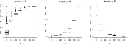
The most interesting plot is in the middle of Figure 1, it shows that the boxplots of ${\hat{D}}_n^{(k)}$'s move up as n increases, ensuring that the fraction of data points such that ${\hat{D}}_n^{(k)}>M_2$ goes to 1 as $n\to \mathrm{\infty }$ for any constant $M_2$. Hence, ${\mathbb{P}}_{{\theta }_n}(\theta \notin B(\hat{\theta },M_2\hat{r}))\to 1$ as $n\to \mathrm{\infty }$, for the chosen deceptive parameter sequence $\{{\theta }_n\}$, which demonstrates the deceptiveness phenomenon.

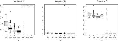
Finally, we perform simulations for the sub-exponential case discussed in Remark 3.3 and a non-deceptive parameter ${\theta }_n^{\prime }=(d_n,\dots ,d_n,0,\dots ,0)\in {\mathbb{R}}^n$. Precisely, we consider the Laplace errors ${\xi }_i\stackrel{\mathrm{ind}}{\sim }\mathrm{Laplac}(1,0)$, $i=1,\dots ,n$ (i.e. with density $\frac{1}{2}{e}^{-|x|}$), we set the first 20 entries of parameter ${\theta }_n^{\prime }$ equal to $d_n$ and the remaining coordinates to zero. This means also that we used complexity $p_{exp}(I)$ instead of $p(I)$. All the other parameters of this simulation experiment remain the same as before.

Figure 2 shows that the claims of Theorems 3.1 and 3.2 hold for non-deceptive $\{{\theta }_n^{\prime }\}$. We now see a downward trend in the boxplots of ${\hat{D}}_n^{(k)}$'s as n increases illustrating the good behaviour of the confidence set for non-deceptive $\{{\theta }_n^{\prime }\}$ also in the sub-exponential case.

Figure 2. Sub-exponential case: boxplots of ${\tilde{D}}_n^{(k)}$'s, ${\hat{D}}_n^{(k)}$'s, ${\overline{D}}_n^{(k)}$'s for increasing n and non-deceptive $\{{\theta }_n^{\prime }\}$.

5. Proofs

In this section, we present the proofs of the theorems.

Proof of Theorem 3.1.

First we introduce some notation. Define the events $E_1=\{\rho (\theta -\hat{\theta })\ge M_{1}r(\theta )\},E_2=\{r(\theta ,\hat{I})\le A_{1}r(\theta )\},E_3=\{\rho ({\mathrm{P}}_{\hat{I}}\xi )\le A_{2}p(\hat{I})\},$where the constants $M_1,A_1,A_2>0$ are to be chosen later. We evaluate the probability of interest ${\mathbb{P}}_{\theta }(E_1)={\mathbb{P}}_{\theta }(\rho (\theta -\hat{\theta })\ge M_{1}r(\theta ))$ as follows: (19) $\begin{array}{rl}{\mathbb{P}}_{\theta }(E_1)& ={\mathbb{P}}_{\theta }(E_1\cap E_2\cap E_3)+{\mathbb{P}}_{\theta }(E_1\cap E_3^c)+{\mathbb{P}}_{\theta }(E_1\cap E_2^c\cap E_3)\\ & =T_1+T_2+T_3.\end{array}$(19) We bound these three probabilities separately.

First we bound $T_1$. Using the properties (3(3) ${\rho }_{\tau }(-x)\le C_{\tau }{\rho }_{\tau }(x),\mathrm{with}{C}_{\tau }=max\{\frac{1-\tau }{\tau },\frac{\tau }{1-\tau }\}=\frac{c_{\tau }}{1-c_{\tau }}.$(3) ) and (4(4) $\rho (x+y)\le \rho (x)+\rho (y),x,y\in {\mathbb{R}}^m.$(4) ) of the quantile loss function ρ, we derive that the event $E_1\cap E_2\cap E_3$ implies that $\begin{array}{rl}{M}_{1}r(\theta )& \le \rho (\theta -\hat{\theta })=\rho (\theta -{\mathrm{P}}_{\hat{I}}X)\\ & \le \rho (\theta -{\mathrm{P}}_{\hat{I}}\theta )+\rho (-{\mathrm{P}}_{\hat{I}}\xi )\le \rho (\theta -{\mathrm{P}}_{\hat{I}}\theta )+A_2{C}_{\tau }p(\hat{I})\\ & \le max\{1,\frac{A_2{C}_{\tau }}{\varkappa }\}r(\theta ,\hat{I})\le max\{1,\frac{A_2{C}_{\tau }}{\varkappa }\}{A}_{1}r(\theta ).\end{array}$Hence, if $M_1>A_{1}max\{1,\frac{A_2{C}_{\tau }}{\varkappa }\}$, then (20) $T_1={\mathbb{P}}_{\theta }(E_1\cap E_2\cap E_3)\le {\mathbb{P}}_{\theta }(M_{1}r(\theta )\le max\{1,\frac{A_2{C}_{\tau }}{\varkappa }\}{A}_{1}r(\theta ))=0.$(20) To bound $T_2$, write $T_2={\mathbb{P}}_{\theta }(E_1\cap E_3^c)\le {\mathbb{P}}_{\theta }(E_3^c)\le {\sum }_{I\in \mathcal{I}}\mathbb{P}(\rho ({\mathrm{P}}_I\xi )>A_{2}p(I)).$If $A_2>0$ is such that $\psi (A_2)>M_0+1$, then using Condition C1 (7(7) $\underset{\theta \in {\mathbb{R}}^n}{sup}{\mathbb{P}}_{\theta }(\rho ({\mathrm{P}}_I\xi )>Mp(I))\le H_0{e}^{-(\psi (M)-M_0)\lambda (|I|)}.$(7) ), we obtain that $\mathbb{P}(\rho ({\mathrm{P}}_I\xi )>A_{2}p(I))\le H_0{e}^{-A_3\lambda (|I|)},I\in \mathcal{I},I\ne \varnothing ,$where we set $A_3=\psi (A_2)-M_0$. Recall that $\lambda (s)$ is increasing for $s\in (0,n]$. This, (6(6) $\sum _{I\in \mathcal{I}}{e}^{-\nu \lambda (|I|)}=1+\sum _{s\in [n]}\sum _{I:|I|=s}{e}^{-\nu \lambda (s)}\le 1+\sum _{s\in [n]}{e}^{-(\nu -1)s}\le C_{\nu },$(6) ) and the two previous displays entail that, since $A_3>1$ (so that $A_4=\frac{(A_3-1)}{2}>0$), (21) $\begin{array}{rl}{T}_2& \le {\mathbb{P}}_{\theta }(E_3^c)\le \sum _{I\in \mathcal{I}}\mathbb{P}(\rho ({\mathrm{P}}_I\xi )>A_{2}p(I))\le H_{\xi }\sum _{I\in \mathcal{I}:|I|\ge 1}{e}^{-A_3\lambda (|I|)}\\ & \le H_{\xi }{e}^{-A_4\lambda (1)}\sum _{I\in \mathcal{I}:|I|\ge 1}{e}^{-(1+A_4)\lambda (|I|)}\le H_1^{\prime }{e}^{-A_4\lambda (1)}.\end{array}$(21) Finally, we bound $T_3={\mathbb{P}}_{\theta }(E_1\cap E_2^c\cap E_3)$. Using (10(10) $\begin{array}{rl}\kappa (p(\hat{I})-p(I^{\prime }))& \le \rho ({\mathrm{P}}_{I^{\prime c}}X)-\rho ({\mathrm{P}}_{{\hat{I}}^c}X)=\rho ({\mathrm{P}}_{\hat{I}\mathrm{\setminus }{I}^{\prime }}X)-\rho ({\mathrm{P}}_{I^{\prime }\mathrm{\setminus }\hat{I}}X)\\ & \le \rho ({\mathrm{P}}_{\hat{I}\mathrm{\setminus }{I}^{\prime }}\theta )+\rho ({\mathrm{P}}_{\hat{I}\mathrm{\setminus }{I}^{\prime }}\xi )-\rho ({\mathrm{P}}_{I^{\prime }\mathrm{\setminus }\hat{I}}\theta )+\rho ({\mathrm{P}}_{I^{\prime }\mathrm{\setminus }\hat{I}}(-\xi ))\\ & \le \rho ({\mathrm{P}}_{I^{\prime c}}\theta )-\rho ({\mathrm{P}}_{{\hat{I}}^c}\theta )+\rho ({\mathrm{P}}_{\hat{I}}\xi )+C_{\tau }\rho ({\mathrm{P}}_{I^{\prime }}\xi ).\end{array}$(10) ) with $I^{\prime }=I_o$ and $\kappa >A_2$, we obtain that under $E_2^c\cap E_3$, $\begin{array}{rl}{C}_{\tau }\rho (P_{I_o}\xi )& \ge \rho ({\mathrm{P}}_{{\hat{I}}^c}\theta )+\kappa p(\hat{I})-\rho ({\mathrm{P}}_{I_o^c}\theta )-\kappa p(I_o)-\rho (P_{\hat{I}}\xi )\\ & \ge \rho ({\mathrm{P}}_{{\hat{I}}^c}\theta )+\kappa p(\hat{I})-\rho ({\mathrm{P}}_{I_o^c}\theta )-\kappa p(I_o)-A_{2}p(\hat{I})\\ & \ge min\{\frac{\kappa -A_2}{\varkappa },1\}r(\theta ,\hat{I})-max\{\frac{\kappa }{\varkappa },1\}r(\theta )\\ & \ge min\{\frac{\kappa -A_2}{\varkappa },1\}{A}_{1}r(\theta )-max\{\frac{\kappa }{\varkappa },1\}r(\theta )\\ & =A_{5}r(\theta )\ge A_5\varkappa p(I_o),\end{array}$as long as $A_5=min\{\frac{\kappa -A_2}{\varkappa },1\}{A}_1-max\{\frac{\kappa }{\varkappa },1\}>0$. We conclude that the event $E_2^c\cap E_3$ implies the event $\{\rho ({\mathrm{P}}_{I_o}\xi )\ge \frac{A_5\varkappa }{C_{\tau }}p(I_o)\}$, so that, by Condition C1 (7(7) $\underset{\theta \in {\mathbb{R}}^n}{sup}{\mathbb{P}}_{\theta }(\rho ({\mathrm{P}}_I\xi )>Mp(I))\le H_0{e}^{-(\psi (M)-M_0)\lambda (|I|)}.$(7) ), (22) $T_3\le {\mathbb{P}}_{\theta }(E_2^c\cap E_3)\le {\mathbb{P}}_{\theta }(\rho ({\mathrm{P}}_{I_o}\xi )\ge \frac{A_5\varkappa }{C_{\tau }}p(I_o))\le H_{\xi }{e}^{-A_6\lambda (1)},$(22) where $A_6=\psi (\frac{A_5\varkappa }{C_{\tau }})-M_0>0$ if $A_5>0$ is chosen so large that $\psi (\frac{A_5\varkappa }{C_{\tau }})>M_0$.

To summarise the choices of the constants, we need to take such $\kappa ,M_1>0$ (in the claim of the theorem) and such constants $A_1,A_2>0$ (in the proof of the theorem) that $M_1>A_{1}max\{1,\frac{A_2{C}_{\tau }}{\varkappa }\}$, $A_3=\psi (A_2)>M_0+1$, $A_5=min\{\frac{\kappa -A_2}{\varkappa },1\}{A}_1-max\{\frac{\kappa }{\varkappa },1\}>0$ (for example, we can fix $\kappa =A_2+1$) and $\psi (\frac{A_5\varkappa }{C_{\tau }})>M_0$, which is always possible since function $\psi (u)\to \mathrm{\infty }$ monotonically as $u\to \mathrm{\infty }$. Combining (19(19) $\begin{array}{rl}{\mathbb{P}}_{\theta }(E_1)& ={\mathbb{P}}_{\theta }(E_1\cap E_2\cap E_3)+{\mathbb{P}}_{\theta }(E_1\cap E_3^c)+{\mathbb{P}}_{\theta }(E_1\cap E_2^c\cap E_3)\\ & =T_1+T_2+T_3.\end{array}$(19) ) –(22(22) $T_3\le {\mathbb{P}}_{\theta }(E_2^c\cap E_3)\le {\mathbb{P}}_{\theta }(\rho ({\mathrm{P}}_{I_o}\xi )\ge \frac{A_5\varkappa }{C_{\tau }}p(I_o))\le H_{\xi }{e}^{-A_6\lambda (1)},$(22) ), we obtain the claim of the theorem with the chosen κ, $M_1$, $H_1=H_1^{\prime }+H_0$ and $m_1=min\{A_4,A_6\}$.

Proof of Theorem 3.2.

For some fixed $\delta \in (0,1)$ (for example, take $\delta =1/2$), introduce the event $E_4=\{p(\hat{I})\le \delta p(I_o)\}$, where $I_o=I_o(\theta )$ is defined by (11(11) $\underset{I\in \mathcal{I}}{min}{r}_{\varkappa }(\theta ,I)=r_{\varkappa }(\theta ,I_o)=r_{\varkappa }(\theta )=r(\theta ).$(11) ).

First we evaluate ${\mathbb{P}}_{\theta }(p(\hat{I})\le \delta p(I_o))={\mathbb{P}}_{\theta }(E_4)$. We have $\begin{array}{rl}p(\hat{I}\cup I_o)& =|\hat{I}\cup I_o|{\log }^{1/2}\left(\frac{en}{|\hat{I}\cup I_o|}\right)\\ & \le |\hat{I}|{\log }^{1/2}\left(\frac{en}{|\hat{I}\cup I_o|}\right)+|I_o|{\log }^{1/2}\left(\frac{en}{|\hat{I}\cup I_o|}\right)\\ & \le |\hat{I}|{\log }^{1/2}\left(\frac{en}{|\hat{I}|}\right)+|I_o|{\log }^{1/2}\left(\frac{en}{|I_o|}\right)\\ & =p(\hat{I})+p(I_o).\end{array}$By using the above relation, we obtain that, under the event $E_4$, $p(\hat{I}\cup I_o)\le p(\hat{I})+p(I_o)\le (1+\delta )p(I_o)$. Hence, we have that, under $E_4$, $\frac{1}{1+\delta }p(\hat{I}\cup I_o)\le p(I_o)\le p(\hat{I}\cup I_o).$The last relation, (5(5) $\mathrm{If}{I}_1\subseteq I_2,\mathrm{then}\rho ({\mathrm{P}}_{I_1}x)\le \rho ({\mathrm{P}}_{I_2}x),x\in {\mathbb{R}}^n.$(5) ) with $I_1=(\hat{I}\cup I_o{)}^c\subseteq I_o^c=I_2$ and the definition (11(11) $\underset{I\in \mathcal{I}}{min}{r}_{\varkappa }(\theta ,I)=r_{\varkappa }(\theta ,I_o)=r_{\varkappa }(\theta )=r(\theta ).$(11) ) of the oracle $I_o$ imply that, under $E_4$, $\begin{array}{rl}\rho ({\mathrm{P}}_{{\hat{I}}^c}\theta )-\rho ({\mathrm{P}}_{(\hat{I}\cup I_o{)}^c}\theta )& \ge \rho ({\mathrm{P}}_{{\hat{I}}^c}\theta )-\rho ({\mathrm{P}}_{I_o^c}\theta )\ge \varkappa (p(I_o)-p(\hat{I}))\\ & \ge \varkappa (1-\delta )p(I_o)\ge \varkappa \frac{1-\delta }{1+\delta }p(\hat{I}\cup I_o).\end{array}$Recall the event $E_3=\{\rho ({\mathrm{P}}_{\hat{I}}\xi )\le A_{2}p(\hat{I})\}$ from the proof of the previous theorem and let κ be sufficiently large to satisfy $\kappa >A_2$. Further, choose ϰ sufficiently large to satisfy $\varkappa \frac{1-\delta }{1+\delta }-\kappa >C_{\tau }{A}_7$ with such $A_7>0$ that $A_8=\psi (A_7)-M_0>0$. Then, under $E_3\cap E_4$, from (10(10) $\begin{array}{rl}\kappa (p(\hat{I})-p(I^{\prime }))& \le \rho ({\mathrm{P}}_{I^{\prime c}}X)-\rho ({\mathrm{P}}_{{\hat{I}}^c}X)=\rho ({\mathrm{P}}_{\hat{I}\mathrm{\setminus }{I}^{\prime }}X)-\rho ({\mathrm{P}}_{I^{\prime }\mathrm{\setminus }\hat{I}}X)\\ & \le \rho ({\mathrm{P}}_{\hat{I}\mathrm{\setminus }{I}^{\prime }}\theta )+\rho ({\mathrm{P}}_{\hat{I}\mathrm{\setminus }{I}^{\prime }}\xi )-\rho ({\mathrm{P}}_{I^{\prime }\mathrm{\setminus }\hat{I}}\theta )+\rho ({\mathrm{P}}_{I^{\prime }\mathrm{\setminus }\hat{I}}(-\xi ))\\ & \le \rho ({\mathrm{P}}_{I^{\prime c}}\theta )-\rho ({\mathrm{P}}_{{\hat{I}}^c}\theta )+\rho ({\mathrm{P}}_{\hat{I}}\xi )+C_{\tau }\rho ({\mathrm{P}}_{I^{\prime }}\xi ).\end{array}$(10) ) with $I^{\prime }=\hat{I}\cup I_o$, it follows that, (23) $\begin{array}{rl}{C}_{\tau }\rho ({\mathrm{P}}_{I_o}\xi )& \ge \kappa (p(\hat{I})-p(I^{\prime }))-A_{2}p(\hat{I})+\rho ({\mathrm{P}}_{{\hat{I}}^c}\theta )-\rho ({\mathrm{P}}_{I^{\prime c}}\theta )\\ & \ge (\varkappa \frac{1-\delta }{1+\delta }-\kappa )p(\hat{I}\cup I_o)\\ & \ge (\varkappa \frac{1-\delta }{1+\delta }-\kappa )p(I_o)>C_{\tau }{A}_{7}p(I_o).\end{array}$(23) Using the last display, (21(21) $\begin{array}{rl}{T}_2& \le {\mathbb{P}}_{\theta }(E_3^c)\le \sum _{I\in \mathcal{I}}\mathbb{P}(\rho ({\mathrm{P}}_I\xi )>A_{2}p(I))\le H_{\xi }\sum _{I\in \mathcal{I}:|I|\ge 1}{e}^{-A_3\lambda (|I|)}\\ & \le H_{\xi }{e}^{-A_4\lambda (1)}\sum _{I\in \mathcal{I}:|I|\ge 1}{e}^{-(1+A_4)\lambda (|I|)}\le H_1^{\prime }{e}^{-A_4\lambda (1)}.\end{array}$(21) ), Condition C1 (7(7) $\underset{\theta \in {\mathbb{R}}^n}{sup}{\mathbb{P}}_{\theta }(\rho ({\mathrm{P}}_I\xi )>Mp(I))\le H_0{e}^{-(\psi (M)-M_0)\lambda (|I|)}.$(7) ) and $A_8=\psi (A_7)-M_0>0$, we bound (24) $\begin{array}{rl}{\mathbb{P}}_{\theta }(p(\hat{I})\le \delta p(I_o))& ={\mathbb{P}}_{\theta }(E_4)\le {\mathbb{P}}_{\theta }(E_3^c)+{\mathbb{P}}_{\theta }(E_3\cap E_4)\\ & \le H_1^{\prime }{e}^{-A_4\lambda (1)}+{\mathbb{P}}_{\theta }(\rho ({\mathrm{P}}_{I_o}\xi )>A_{7}p(I_o))\\ & \le H_1^{\prime }{e}^{-A_4\lambda (1)}+H_0{e}^{-A_8\lambda (1)}.\end{array}$(24) Now we establish the coverage property. The constants $M_1$, $H_1$ and $m_1$ are defined in Theorem 3.1. Take $M_2=\frac{M_1(t+\varkappa )}{\delta }$, where fixed $\delta \in (0,1)$ is from the definition of the event $E_4$. If $\theta \in {\mathrm{\Theta }}_{\mathrm{eb}}(t)$, then, in view of (11(11) $\underset{I\in \mathcal{I}}{min}{r}_{\varkappa }(\theta ,I)=r_{\varkappa }(\theta ,I_o)=r_{\varkappa }(\theta )=r(\theta ).$(11) ), $r(\theta )=\rho ({\mathrm{P}}_{I_o^c}\theta )+\varkappa p(I_o)\le (t+\varkappa )p(I_o)$. So, $p(I_o)\ge (t+\varkappa {)}^{-1}r(\theta )$ for all $\theta \in {\mathrm{\Theta }}_{\mathrm{eb}}(t)$. Combining this with Theorem 3.1 and (24(24) $\begin{array}{rl}{\mathbb{P}}_{\theta }(p(\hat{I})\le \delta p(I_o))& ={\mathbb{P}}_{\theta }(E_4)\le {\mathbb{P}}_{\theta }(E_3^c)+{\mathbb{P}}_{\theta }(E_3\cap E_4)\\ & \le H_1^{\prime }{e}^{-A_4\lambda (1)}+{\mathbb{P}}_{\theta }(\rho ({\mathrm{P}}_{I_o}\xi )>A_{7}p(I_o))\\ & \le H_1^{\prime }{e}^{-A_4\lambda (1)}+H_0{e}^{-A_8\lambda (1)}.\end{array}$(24) ) yields that, uniformly in $\theta \in {\mathrm{\Theta }}_{\mathrm{eb}}(t)$, $\begin{array}{rl}& {\mathbb{P}}_{\theta }(\theta \notin B(\hat{\theta },M_2\hat{r}))\\ & \le {\mathbb{P}}_{\theta }(\rho (\theta -\hat{\theta })>M_2\hat{r},\hat{r}\ge \delta p(I_o))+{\mathbb{P}}_{\theta }(\hat{r}<\delta p(I_o))\\ & \le {\mathbb{P}}_{\theta }(\rho (\theta -\hat{\theta })>M_1(t+\varkappa )p(I_o))+{\mathbb{P}}_{\theta }(p(\hat{I})<\delta p(I_o))\\ & \le {\mathbb{P}}_{\theta }(\rho (\theta -\hat{\theta })>M_{1}r(\theta ))+{\mathbb{P}}_{\theta }(p(\hat{I})<\delta p(I_o))\\ & \le H_1{e}^{-m_1\lambda (1)}+H_1^{\prime }{e}^{-A_4\lambda (1)}+H_0{e}^{-A_8\lambda (1)}.\end{array}$The coverage relation follows.

Let us show the size property. Recall again the event $E_3=\{\rho ({\mathrm{P}}_{\hat{I}}\xi )\le A_{2}p(\hat{I})\}$ from the proof of the previous theorem. By using (23(23) $\begin{array}{rl}{C}_{\tau }\rho ({\mathrm{P}}_{I_o}\xi )& \ge \kappa (p(\hat{I})-p(I^{\prime }))-A_{2}p(\hat{I})+\rho ({\mathrm{P}}_{{\hat{I}}^c}\theta )-\rho ({\mathrm{P}}_{I^{\prime c}}\theta )\\ & \ge (\varkappa \frac{1-\delta }{1+\delta }-\kappa )p(\hat{I}\cup I_o)\\ & \ge (\varkappa \frac{1-\delta }{1+\delta }-\kappa )p(I_o)>C_{\tau }{A}_{7}p(I_o).\end{array}$(23) ) with $I^{\prime }=I_o$, we derive that the event $\{p(\hat{I})\ge M_{3}r(\theta )\}\cap E_3$ implies the event $\{C_{\tau }\rho ({\mathrm{P}}_{I_o}\xi )\ge (\kappa -A_2)p(\hat{I})-r(\theta )\le A_{9}p(\hat{I})\ge A_9{M}_{3}r(\theta )\ge A_9{M}_3\varkappa p(I_o)\}$ with $A_9=\kappa -A_2-M_3^{-1}>0$, where $A_2$ is defined in the proof of Theorem 3.1. We thus have that, for any $\theta \in {\mathbb{R}}^n$, $\begin{array}{rl}{\mathbb{P}}_{\theta }(\hat{r}\ge M_{3}r(\theta ))& \le {\mathbb{P}}_{\theta }(E_3^c)+{\mathbb{P}}_{\theta }(\hat{r}\ge M_{3}r(\theta ),E_3)\\ & ={\mathbb{P}}_{\theta }(E_3^c)+{\mathbb{P}}_{\theta }(p(\hat{I})\ge M_{3}r(\theta ),E_3)\\ & \le {\mathbb{P}}_{\theta }(E_3^c)+{\mathbb{P}}_{\theta }(p(\hat{I})\ge M_{3}r(\theta ),C_{\tau }\rho ({\mathrm{P}}_{I_o}\xi )\ge A_{9}p(\hat{I}))\\ & \le {\mathbb{P}}_{\theta }(E_3^c)+{\mathbb{P}}_{\theta }(C_{\tau }\rho ({\mathrm{P}}_{I_o}\xi )\ge A_{9}p(\hat{I})\ge A_9{M}_3\varkappa p(I_o))\\ & \le H_1^{\prime }{e}^{-A_4\lambda (1)}+H_0{e}^{-A_{10}\lambda (1)},\end{array}$where the last inequality in the above display is obtained by (21(21) $\begin{array}{rl}{T}_2& \le {\mathbb{P}}_{\theta }(E_3^c)\le \sum _{I\in \mathcal{I}}\mathbb{P}(\rho ({\mathrm{P}}_I\xi )>A_{2}p(I))\le H_{\xi }\sum _{I\in \mathcal{I}:|I|\ge 1}{e}^{-A_3\lambda (|I|)}\\ & \le H_{\xi }{e}^{-A_4\lambda (1)}\sum _{I\in \mathcal{I}:|I|\ge 1}{e}^{-(1+A_4)\lambda (|I|)}\le H_1^{\prime }{e}^{-A_4\lambda (1)}.\end{array}$(21) ) and Condition C1 (7(7) $\underset{\theta \in {\mathbb{R}}^n}{sup}{\mathbb{P}}_{\theta }(\rho ({\mathrm{P}}_I\xi )>Mp(I))\le H_0{e}^{-(\psi (M)-M_0)\lambda (|I|)}.$(7) ), and $M_3$ is chosen to be so large that $A_{10}=\psi (A_9{M}_3\varkappa /C_{\tau })-M_0>0$. The size relation follows.

Disclosure statement

No potential conflict of interest was reported by the author(s).

References

- Abramovich, F., Benjamini, Y., Donoho, D.L., and Johnstone, I.M. (2006), ‘Adapting to Unknown Sparsity by Controlling the False Discovery Rate’, The Annals of Statistics, 34, 584–653.
- Abrevaya, J. (2002), ‘The Effects of Demographics and Maternal Behavior on the Distribution of Birth Outcomes’, in Economic Applications of Quantile Regression, eds. B. Fitzenberger, R. Koenker, and J. A. F. Machado, Berlin Heidelberg: Springer-Verlag, pp. 247–257.
- Babenko, A., and Belitser, E. (2010), ‘Oracle Convergence Rate of Posterior Under Projection Prior and Bayesian Model Selection’, Mathematical Methods of Statistics, 19, 219–245.
- Baraud, Y. (2004), ‘Confidence Balls in Gaussian Regression’, The Annals of Statistics, 32, 528–551.
- Belitser, E. (2017), ‘On Coverage and Local Radial Rates of Credible Sets’, The Annals of Statistics, 45, 1124–1151.
- Belitser, E., and Ghosal, S. (2020), ‘Empirical Bayes Oracle Uncertainty Quantification for Regression’, The Annals of Statistics, 31, 536–559.
- Belitser, E., and Nurushev, N. (2019), General Framework for Projection Structures. ArXiv: 1904.01003.
- Belitser, E., and Nurushev, N. (2020), ‘Needles and Straw in a Haystack: Robust Empirical Bayes Confidence for Possibly Sparse Sequences’, Bernoulli, 26, 191–225.
- Bellec, P.C. (2018), ‘Sharp Oracle Inequalities for Least Squares Estimators in Shape Restricted Regression’, The Annals of Statistics, 46, 745–780.
- Belloni, A., and Chernozhukov, V. (2011), ‘L1-Penalized Quantile Regression in High-Dimensional Sparse Models’, The Annals of Statistics, 39, 82–130.
- Belloni, A., Chernozhukov, V., and Kato, K. (2019), ‘Valid Post-Selection Inference in High-Dimensional Approximately Sparse Quantile Regression Models’, Journal of the American Statistical Association, 114, 749–758.
- Belloni, A., Chernozhukov, V., and Wang, L. (2011), ‘Square-root Lasso: Pivotal Recovery of Sparse Signals via Conic Programming’, Biometrika, 98, 791–806.
- Benjamini, Y., and Hochberg, Y. (1995), ‘Controlling the False Discovery Rate: A Practical and Powerful Approach to Multiple Testing’, Journal of the Royal Statistical Society: Series B, 57, 289–300.
- Birgé, L., and Massart, P. (2001), ‘Gaussian Model Selection’, Journal of the European Mathematical Society, 3, 203–268.
- Butucea, C., Ndaoud, M., Stepanova, N., and Tsybakov, A. (2018), ‘Variable Selection with Hamming Loss’, The Annals of Statistics, 46, 1837–1875.
- Castillo, I., and van der Vaart, A. (2012), ‘Needles and Straw in a Haystack: Posterior Concentration for Possibly Sparse Sequences’, The Annals of Statistics, 40, 2069–2101.
- Donoho, D.L., and Johnstone, I.M. (1994), ‘Minimax Risk Over ℓp-Balls for ℓq-Error’, Probability Theory and Related Fields, 99, 277–303.
- Donoho, D.L., Johnstone, I.M., Hoch, J.C., and Stern, A.S. (1992), ‘Maximum Entropy and the Nearly Black Object (with Discussion)’, Journal of the Royal Statistical Society: Series B, 54, 41–81.
- Efron, B. (2008), ‘Microarrays, Empirical Bayes and the Two-Groups Model’, Statistical Science, 23, 1–22.
- Gabriela Ciuperca, G. (2018), ‘Test by Adaptive Lasso Quantile Method for Real-Time Detection of a Change-Point’, Metrika, 81, 689–720.
- Hulmán, A., Witte, D.R., Kerényi, Z, Madarász, E., Tánczer, T., Bosnyák, Z, Szabó, E., Ferencz, V., Péterfalvi, A., Tabák, A.G, and Nyári, T.A. (2015), ‘Heterogeneous Effect of Gestational Weight Gain on Birth Weight: Quantile Regression Analysis From a Population-Based Screening’, Annals of Epidemiology, 25, 133–137.
- Jiang, L., Bondell, H.D., and Wang, H.J. (2014), ‘Interquantile Shrinkage and Variable Selection in Quantile Regression’, Computational Statistics & Data Analysis, 69, 208–219.
- Jiang, L., Wang, H.J., and Bondell, H.D. (2013), ‘Interquantile Shrinkage in Regression Models’, Journal of Computational and Graphical Statistics, 22, 970–986.
- Johnstone, I.M. (2017), Gaussian Estimation: Sequence and Wavelet Models, Book Draft.
- Johnstone, I.M., and Silverman, B.W. (2004), ‘Needles and Straw in Haystacks: Empirical Bayes Estimates of Possibly Sparse Sequences’, The Annals of Statistics, 32, 1594–1649.
- Koenker, R. (2005), Quantile Regression, Cambridge: Cambridge University Press.
- Li, K.-C. (1989), ‘Honest Confidence Regions for Nonparametric Regression’, The Annals of Statistics, 17, 1001–1008.
- Martin, R., and Walker, S.G. (2014), ‘Asymptotically Minimax Empirical Bayes Estimation of a Sparse Normal Mean Vector’, Electronic Journal of Statistics, 8, 2188–2206.
- Santosa, F., and Symes, W.W. (1986), ‘Linear Inversion of Band-Limited Reflection Seismograms’, SIAM Journal on Scientific and Statistical Computing, 7, 1307–1330.
- Szabó, B.T., van der Vaart, A.W., and van Zanten, J.H. (2015), ‘Frequentist Coverage of Adaptive Nonparametric Bayesian Credible Sets’, The Annals of Statistics, 43, 1391–1428.
- van der Pas, S.L., Szabó, B.T., and van der Vaart, A.W. (2017), ‘Uncertainty Quantification for the Horseshoe (with Discussion)’, Bayesian Analysis, 12, 1221–1274.
- Vershynin, R. (2018), High-Dimensional Probability. An Introduction with Applications in Data Science, Cambridge: Cambridge University Press.
- Zou, H., and Yuan, M. (2008), ‘Composite Quantile Regression and the Oracle Model Selection Theory’, The Annals of Statistics, 36, 1108–1126.