On estimation of covariance function for functional data with detection limits

Abstract

In many studies on disease progression, biomarkers are restricted by detection limits, hence informatively missing. Current approaches ignore the problem by just filling in the value of the detection limit for the missing observations for the estimation of the mean and covariance function, which yield inaccurate estimation. Inspired by our recent work [Liu and Houwing-Duistermaat (2022), ‘Fast Estimators for the Mean Function for Functional Data with Detection Limits’, Stat, e467.] in which novel estimators for mean function for data subject to detection limit are proposed, in this paper, we will propose a novel estimator for the covariance function for sparse and dense data subject to a detection limit. We will derive the asymptotic properties of the estimator. We will compare our method to the standard method, which ignores the detection limit, via simulations. We will illustrate the new approach by analysing biomarker data subject to a detection limit. In contrast to the standard method, our method appeared to provide more accurate estimates of the covariance. Moreover its computation time is small.

Keywords:

• Functional data analysis
• informative missing
• detection limit
• local constant covariance estimation

Mathematics Subject Classifications:

• 62G05
• 62G20
• 62N01

1. Introduction

Technological advances resulted in a growing number of datasets containing temporal observations, either dense or sparse. For analysis of these data, functional data analysis (FDA) methods have been developed, see, for example Ramsay and Silverman (2005), Ferraty and Vieu (2006), Horváth and Kokoszka (2012) and Kokoszka and Reimherr (2017) for dense data and Yao, Müller, and Wang (2005), Peng and Paul (2009), Li and Hsing (2010), Wang, Chiou, and Müller (2016) and Zhang and Wang (2016) for sparse data. These methods assume that there is no missing data. However, in practice, we may have data subject to detection limits. Recently, several methods for the estimation of the mean function have been proposed and investigated when the data are subject to detection limits, namely the global method by Shi, Dong, Wang, and Cao (2021) and several local methods by Liu and Houwing-Duistermaat (2022). However, an estimator for the covariance has not yet been developed, which is the topic of this paper.

When levels of a specific marker in a sample have to be determined in a laboratory, we often deal with detection limits. The amount of the marker might be too low to be detected. This results in too many zeros in the dataset and an observed ‘zero’ might be a true zero or just very small. Also on the other extreme of the distribution, detection limits might occur, since measurement techniques are often optimised for a certain range of values and values above and below a certain threshold cannot be accurately measured. Detection limits are not restricted to laboratory measurements. Devices which measure certain characteristics (number of steps for example) might be out of charge yielding an underestimation of the characteristic per day (e.g. the true number of steps for a day is higher than the measured number of steps if the device was out of charge). For simplicity in this paper, we only consider detection limits on the lower extreme of the distribution, i.e. we do not observe values lower than a specific value, instead we observe this specific value which is also called detection limit (DL).

For observations subject to DL, Shi et al. (2021) proposed a global method. However, since observations close to the target point t contain more information about the mean function at t than observations far away from t, local methods as proposed by Liu and Houwing-Duistermaat (2022) might be more appropriate. The estimator of Liu and Houwing-Duistermaat (2022) is based on approximations of the likelihood function. For data subject to DL, the likelihood function is a product of probability density functions for the observed values and of probability distribution functions for the observations subject to DL, since for the latter observations we know that the unobserved value is below a known threshold. To estimate the mean function around observed time points, the authors proposed to use the local polynomial kernel method (Fan and Gijbels 1995, 2018; Beran and Liu 2014, 2016). Further two weighting schemes for subjects have been considered (Zhang and Wang 2016; Liu and Houwing-Duistermaat 2022), namely the SUBJ scheme which assigns the same weight to each subject and the OBS scheme which assigns the same weight to each observation. The latter scheme will assign more weight to subjects with more observations. To reduce the computation time, Liu and Houwing-Duistermaat (2022) proposed linear and constant approximations for the probability distribution functions in the likelihood function. The constant approximation is computationally fast especially for dense data while it only performs slightly less than the exact and linear approximation method. Note that the global method of Shi et al. (2021) is even more computational inefficient than the linear approximation for dense data. Therefore, in this paper we will use constant approximations to obtain an estimator for the covariance function.

We propose a local constant estimator with approximation and derive their asymptotic behaviour. Via simulations we evaluate their performance in a sparse and a dense setting under both SUBJ and OBS weighting schemes and compare their performance with the standard method where the detection limit is used for the missing values. We also investigate the asymptotic behaviour of the estimators via simulations. To illustrate the proposed method, we apply it to temporal data from a biomarker study. We finish with a conclusion.

2. Methodology

2.1. Functional principal component analysis (FPCA)

We first define the model for functional data subject to a detection limit. Let $\{X(t):t\in I\}$ be an $L^2$ stochastic process on interval I. Let $\mu (t)=E[X(t)]$ and $C(s,t)=E[(X(s)-\mu (s))(X(t)-\mu (t))]$ be the mean and covariance function of $X(t)$, respectively. Then $X(t)$ can be decomposed into $X(t)=\mu (t)+U(t)$where $U(t)$ is the stochastic part of $X(t)$ which has mean zero, i.e. $E[U(t)]=0$ for $t\in I$, and covariance $C(s,t)=E[U(s)U(t)]$ for all $s,t\in I$. By Karhunen–Loeve expansion and Mercer's Theorem, we have $C(s,t)=\sum _{l=1}^{\mathrm{\infty }}{\lambda }_l{\psi }_l(s){\psi }_l(t)$and $U(t)=\sum _{l=1}^{\mathrm{\infty }}{\xi }_l{\psi }_l(t),$where ${\psi }_l(t)$ are eigenfunctions of the covariance operator corresponding to $C(s,t)$, positive real numbers ${\lambda }_1>{\lambda }_2>\cdots$ are the eigenvalues of the covariance operator corresponding to $C(s,t)$, and $var({\xi }_l)={\lambda }_l$. Note that the functional principal components $\{{\psi }_l(t)\}$ (FPCs) are an orthonormal basis for $L^2(I)$.

Let $X_1(t),\dots ,X_n(t)$ be n iid copies of $X(t)$ with $t\in I$. We have observations of $X_1(t),\dots ,X_n(t)$ at discrete time points $t_{i1},\dots ,t_{i{N}_i}$ perturbed by an independent random error. Here, $N_i$ is the number of measurements for subject i Specifically, let $Y_{ij}$ denote the random variable for the jth time point for subject i with $j=1,\dots ,N_i$ and $i=1,\dots ,n$. We can model $Y_{ij}$ as follows: (1) $Y_{ij}=X_i(t_{ij})+{ϵ}_{ij}=\mu (t_{ij})+U_i(t_{ij})+{ϵ}_{ij}=\mu (t_{ij})+\sum _{l=1}^{\mathrm{\infty }}{\xi }_{il}{\psi }_l(t_{ij})+{ϵ}_{ij}$(1) where ${ϵ}_{ij}$ is an independent random measurement error term following a distribution in the exponential family with mean zero and variance ${\sigma }^2$ that is, ${ϵ}_{ij}$ are independent for any i and j. We assume further that ${ϵ}_{ij}$ is independent of $U_i(t)$ (or equivalently ${\xi }_{il}$). Often a Gaussian distribution is assumed, i.e. we have ${ϵ}_{ij}\sim \mathcal{N}(0,{\sigma }^2)$ and ${\xi }_{il}\sim \mathcal{N}(0,{\lambda }_l)$.

Now, not all $Y_{ij}$ are observed due to the presence of a DL. Let ${\delta }_{ij}$ be the missingness indicator, i.e. ${\delta }_{ij}=0$ if $Y_{ij}$ is observed, and ${\delta }_{ij}=1$ if $Y_{ij}$ is unobserved. If ${\delta }_{ij}=1$, we assume that the unobserved $Y_{ij}$ has a value smaller than (or equal to) a specific threshold $c_{ij}$. For the sake of simplicity of notation, we assume the threshold is fixed, i.e. $c_{ij}=c$ for all i, j. Therefore, the observations are $\{(t_{ij},y_{ij},{\delta }_{ij})\},i=1,\dots ,n,j=1,\dots ,N_i,$where $y_{ij}$ is missing for ${\delta }_{ij}=1$.

The consequence of the presence of a DL is that in the likelihood function the contributions of the observations subject to the DL are represented by the probability distribution function instead of the density function. As a consequence the likelihood function is hard to maximise. Liu and Houwing-Duistermaat (2022) proposed to locally approximate the probability distributions by a linear function or by a constant resulting in time efficient estimators for the mean function. They showed via simulations that the local-linear estimator performed only slightly better than the local-constant estimator, but was less time efficient. Therefore, in this paper we will only consider the local-constant estimator.

2.2. Locally Kernel weighted log-likelihood estimator for the mean function

In this section, we briefly summarise the estimation procedure of the mean function which was developed by Liu and Houwing-Duistermaat (2022). For this section, without loss of generalisability, we assume that $U(t)=0$ in formula (1(1) $Y_{ij}=X_i(t_{ij})+{ϵ}_{ij}=\mu (t_{ij})+U_i(t_{ij})+{ϵ}_{ij}=\mu (t_{ij})+\sum _{l=1}^{\mathrm{\infty }}{\xi }_{il}{\psi }_l(t_{ij})+{ϵ}_{ij}$(1) ), i.e. we ignore the covariance between $X(t)$ at various time points. The loglikelihood function approximated locally by a constant is as follows (see Liu and Houwing-Duistermaat 2022): (2) $\begin{array}{rl}L(\mathit{\beta };h,t)& =\sum _{i=1}^n{w}_i\sum _{j=1}^{N_i}[-0.251{\delta }_{ij}{\left(\frac{c-{\beta }_0}{\sigma }\right)}^2+0.8194{\delta }_{ij}\frac{c-{\beta }_0}{\sigma }\\ & +(0.5-0.5{\delta }_{ij}){\left(\frac{y_{ij}-{\beta }_0}{\sigma }\right)}^2]K_h(t_{ij}-t).\end{array}$(2) where $K_h(\cdot )=\frac{1}{h}K(\frac{\cdot }{h})$ and $K(\cdot )$ is a kernel function see details in Assumption (A1) and $w_i$ are weights. Two types of weights $w_i$ are considered, namely $w_i^{SUBJ}=\frac{1}{n{N}_i}$and $w_i^{OBS}=\frac{1}{\sum _{i=1}^n{N}_i}.$Using loglikelihood function (2(2) $\begin{array}{rl}L(\mathit{\beta };h,t)& =\sum _{i=1}^n{w}_i\sum _{j=1}^{N_i}[-0.251{\delta }_{ij}{\left(\frac{c-{\beta }_0}{\sigma }\right)}^2+0.8194{\delta }_{ij}\frac{c-{\beta }_0}{\sigma }\\ & +(0.5-0.5{\delta }_{ij}){\left(\frac{y_{ij}-{\beta }_0}{\sigma }\right)}^2]K_h(t_{ij}-t).\end{array}$(2) ), Liu and Houwing-Duistermaat (2022) obtained the following local constant estimator of the mean function: (3) ${\hat{\mu }}^{LC}(t)={\hat{\beta }}_0=\frac{R_0}{S_0},$(3) where $S_0=\sum _{i=1}^n{w}_i\sum _{j=1}^{N_i}(1-0.498{\delta }_{ij})K_h(t_{ij}-t)$and $R_0=\sum _{i=1}^n{w}_i\sum _{j=1}^{N_i}[-0.8194{\delta }_{ij}\sigma +0.502{\delta }_{ij}c+(1-{\delta }_{ij})y_{ij}]K_h(t_{ij}-t).$Note that Liu and Houwing-Duistermaat (2022) only derived the asymptotic distribution of the local linear estimator (see Theorem 2.1 of their paper). The asymptotic distribution of ${\hat{\mu }}^{LC}(t)$ given in (3(3) ${\hat{\mu }}^{LC}(t)={\hat{\beta }}_0=\frac{R_0}{S_0},$(3) ) can be obtained in a similar way. In this paper, we derive estimators for the covariance function $C(s,t)$ using similar ideas.

2.3. Local Kernel weighted estimation of covariance function

In this section, we assume $\mu (t)=0$ and $ϵ\sim \mathcal{N}(0,{\sigma }^2)$ (for simplicity of notations). We propose the following fast local constant kernel weighted estimator of $C(s,t)$: (4) $\hat{C}(s,t)=\frac{R_{00}}{S_{00}}$(4) where $R_{00}=\sum _{i=1}^n{v}_i\sum _{1\le j\ne l\le N_i}{K}_h(t_{ij}-s)K_h(t_{il}-t)C_{ijl}$and $S_{00}=\sum _{i=1}^n{v}_i\sum _{1\le j\ne l\le N_i}{K}_h(t_{ij}-s)K_h(t_{il}-t)D_{ijl}$with $C_{ijl}=[-0.8194{\delta }_{ij}\sigma +0.502{\delta }_{ij}c+(1-{\delta }_{ij})y_{ij}]\cdot [-0.8194{\delta }_{il}\sigma +0.502{\delta }_{il}c+(1-{\delta }_{il})y_{il}]$and $D_{ijl}=(1-0.498{\delta }_{ij})(1-0.498{\delta }_{il})$and $v_i$ $v_i^{OBS}=\frac{1}{\sum N_i(N_i-1)}\mathrm{or}{v}_i^{SUBJ}=\frac{1}{n{N}_i(N_i-1)}.$

Remark 2.1

Note that, without DL, the local constant smoother (or NW) for the mean function is $\hat{\mu }(t)={\hat{\beta }}_0=\arg min\sum _{i=1}^n{w}_i\sum _{j=1}^{N_i}(y_{ij}-{\beta }_0{)}^2{K}_h(t_{ij}-t)=\frac{R_0}{S_0}$with ${\delta }_{ij}=0$ for all i and j in $R_0$ and $S_0$ (in formula (3(3) ${\hat{\mu }}^{LC}(t)={\hat{\beta }}_0=\frac{R_0}{S_0},$(3) )), and the local constant smoother for covariance is $\hat{C}(s,t)={\hat{\beta }}_0=\arg min\sum _{i=1}^n{v}_i\sum _{1\le j\ne l\le N_i}(C_{ijl}-{\beta }_0{)}^2{K}_h(t_{ij}-s)K_h(t_{il}-t)=\frac{R_{00}}{S_{00}}$with ${\delta }_{ij}=0$ for all i and j in $R_{00}$ and $S_{00}$ (in formula (4(4) $\hat{C}(s,t)=\frac{R_{00}}{S_{00}}$(4) )).

Remark 2.2

If $\mu (t)$ is unknown, it can be estimated by formula (3(3) ${\hat{\mu }}^{LC}(t)={\hat{\beta }}_0=\frac{R_0}{S_0},$(3) ). Then we can just replace $y_{ij}$ by $y_{ij}-\hat{\mu }(t_{ij})$ in formula (4(4) $\hat{C}(s,t)=\frac{R_{00}}{S_{00}}$(4) ) to obtain the estimate of $C(s,t)$.

For the observations $y_{ij}$, we have that they are observed values of a perturbed underlying continuous function $X(t)$. Now, for ${\delta }_{ij}$, we define indicator functions $\{{\delta }_i(t),i=1,\dots ,n\}$ on interval I with range $\{0,1\}$ and ${\delta }_i(t_{ij})={\delta }_{ij}$. For the covariance estimator defined in Equation (4(4) $\hat{C}(s,t)=\frac{R_{00}}{S_{00}}$(4) ), Theorem 2.1 holds.

Theorem 2.1

Under Assumptions B.1–B.3 given in the Appendix, for a fixed interior point $(s,t)\in I\times I$, $({\mathrm{\Gamma }}_{n,N_i}{)}^{-1/2}[\hat{C}(s,t)-C(s,t)-B(s,t){\sigma }^2-\frac{h^2}{2}{\sigma }_K^{2}D(s,t)+o(h^2)]\to \mathcal{N}(0,1)$where $\begin{array}{rl}{\mathrm{\Gamma }}_{n,N_i}& =\frac{1}{{(\sum N_i(N_i-1)w_{i2}(s,t)f(s)f(t))}^2}\\ & \times (\sum (w_{i1}(s,t)-B(s,t)w_{i2}(s,t){)}^2{\sigma }^4{V}_i^I(s,t)\\ & +\sum w_{i4}^2(s,t){\sigma }^2{V}_i^{II}(s,t)+2\sum w_{i4}(s,t)w_{i4}(t,s){\sigma }^2{V}_i^{III}(s,t)\\ & +2\sum w_{i2}(s,t)w_{i4}(s,t)\sigma V_i^{IV}(s,t)+\sum w_{i4}^2(t,s){\sigma }^2{V}_i^{II}(t,s)\\ & +2\sum w_{i2}(t,s)w_{i4}(t,s)\sigma V_i^{IV}(t,s)+\sum w_{i2}^2(s,t)V_i^V(s,t)),\\ B(s,t)& =\frac{\sum _i{N}_i(N_i-1)w_{i1}(s,t)}{\sum _i{N}_i(N_i-1)w_{i2}(s,t)},\\ D(s,t)& =\frac{2\mathrm{\partial }C(s,t)}{\mathrm{\partial }s}\frac{f^{\mathrm{\prime }}(s)}{f(s)}+\frac{2\mathrm{\partial }C(s,t)}{\mathrm{\partial }t}\frac{f^{\mathrm{\prime }}(t)}{f(t)}+\frac{{\mathrm{\partial }}^{2}C(s,t)}{\mathrm{\partial }{s}^2}+\frac{{\mathrm{\partial }}^{2}C(s,t)}{\mathrm{\partial }{t}^2},\end{array}$$w_{i1}(s,t)$, $w_{i2}(s,t)$, $w_{i3}(s,t)$, and $w_{i4}(s,t)$ are coefficient functions which are defined in Appendix, $V_i^I(s,t)$, $V_i^{II}(s,t)$, $V_i^{III}(s,t)$, $V_i^{IV}(s,t)$ and $V_i^V(s,t)$ are covariance functions which are also defined in Appendix, and notations ${\sigma }_K^2$ and $f(t)$ are also defined in Appendix.

Proof.

The proof comprises showing that the asymptotic bias and the asymptotic variance of $\hat{C}(s,t)$ are equal to $B(s,t){\sigma }^2+\frac{h^2}{2}{\sigma }_K^{2}D(s,t)+o(h^2)$ and ${\mathrm{\Gamma }}_{n,N_i}$ respectively. Here, Assumptions on the kernel (A1), the local polynomial smoothing (B1), (B2) and (B3). Details are given in Appendix. The additional assumption (C1) assures that the asymptotic bias is bounded, and assumption (C2) guarantees that the variance of the estimator goes to zero. The final step is to prove asymptotic normality of $\hat{C}(s,t)$. Note that this follows from the asymptotic normality of $(R_{00}-E[R_{00}],S_{00}-E[S_{00}])$ by the application of the delta method see Theorem 1.12 in Shao (2003). Now, asymptotic normality of $(R_{00}-E[R_{00}],S_{00}-E[S_{00}])$ follows from the Lyapunov condition and Cramer–Wold device. Specifically, Lyapunov CLT of $S_{00}$ and $R_{00}$ can be achieved by the Lyapunov condition given in Assumption (C3), where the power is 3 (i.e. $2+\delta$ and δ is 1) using the notation in Theorem 27.3 in Billingsley (2008). Then the asymptotic joint normality of $(R_{00}-E[R_{00}],S_{00}-E[S_{00}])$ can be derived via the Cramer–Wold device for the two-dimension case, see Theorem 29.4 in Billingsley (2008).

This completes the proof.

Remark 2.3

If there are no observations subject to DL, i.e. ${\delta }_{ij}=0$, for all i, j, then $B(s,t)=0$. Moreover, ${\mathrm{\Gamma }}_{n,N_i}=\frac{1}{f^2(s)f^2(t)}\sum v_i^2{V}_i^V(s,t),$which corresponds to the results of classic local constant covariance estimator (see Zhang and Wang 2016).

3. Simulation study

We evaluate the performance of our proposed estimator of $C(s,t)$ via simulations. We compare its performance with a standard method where the missing observations are replaced with the DL value (Yao et al. 2005). We compare the methods in terms of bias, efficiency, asymptotic behaviour and computation time.

We assume that $\mu (t)=0$ for simplicity and define the true zero mean random function $X(t)$ as follows: $X(t)=\xi \psi (t),t\in [0,1],$where $\psi (t)=\sqrt{2}\cos (4\pi t)$, ξ is a normal random variable with mean zero and variance 2, i.e. $\xi \sim \mathcal{N}(0,\lambda )$ and $\lambda =2$. Therefore the covariance function is $C(s,t)=\lambda \psi (s)\psi (t)=4\cos (4\pi s)\cos (4\pi t),s,t\in [0,1].$The observed time points $t_{ij}\sim \mathcal{U}[0,1]$ are iid sampled from the continuous uniform distribution in the interval $[0,1]$. Additive errors are sampled from ${ϵ}_{ij}\sim \mathcal{N}(0,1)$. Then the response is generated by $Y_{ij}=X_i(t_{ij})+{ϵ}_{ij}={\xi }_i\psi (t_{ij})+{ϵ}_{ij},i=1,\dots ,n,j=1,\dots ,N_i.$Finally, the missing data are created with the observations less than DL are replaced by DL, with DL$=\{-1,0\}$.

We consider two settings, namely a sparse and a dense grid for the observations for each subject i. We, specifically, sample the number of time points $N_i$ for each trajectory i as follows:

• Sparse setting: $N_i\sim \mathcal{U}\{3,4,5,6,7,8,9,10\}$ i.e. $N_i$ are iid from a discrete uniform distribution in $\{3,4,\dots ,10\}$.

• Dense setting: $N_i\sim \mathcal{U}\{75,76,\dots ,100\}$ i.e. $N_i$ iid from a discrete uniform distribution in in $\{75,76,\dots ,100\}$.

For each setting, we simulate Q = 100 replicates. Each replicate contains information of n = 100 subjects.

To estimate the covariance functions in the replicates, we consider the following methods:

• Our estimator based on local constant approximations using either the OBS or the SUBJ weighting schemes.

• PACE which does not adjust for the detection limit (Yao et al. 2005).

For each replicate, the covariance functions are estimated on 20 equal-distant time points in $[0,1]\times [0,1]$. The variance of ${ϵ}_{ij}$ is estimated as the mean squared error based on the least-squared fit using all the data (including the values subject to DL). We use the Gaussian kernel for the estimation procedure. To select the bandwidth h, the integrated squared error (ISE) is computed for a dense grid of values, namely $h=(2:12)/200$. The ISE is defined as follows: $ISE(\hat{C}(s,t),h)={\int }_0^1{\int }_0^1({\hat{C}}_h(s,t)-C(s,t){)}^2\mathrm{d}s\mathrm{d}t,$where ${\hat{C}}_h(s,t)$ is the estimation of C with bandwidth h. The bandwidth which minimises $ISE(\hat{C}(s,t),h)$ is selected as the optimal bandwidth and the corresponding ISE is denoted with $IS{E}_{opt}(\hat{C}(s,t))$ (see Fan and Gijbels 2018).

We then calculate the mean integrated squared error (MISE) and the standard deviation of ISE over $Q(=100)$ replicates: (5) $\begin{array}{rl}MISE(\hat{C}(s,t))& =\frac{1}{Q}\sum _{i=1}^{Q}IS{E}_{opt}({\hat{C}}^{([i])}(s,t)),\end{array}$(5) (6) $\begin{array}{rl}SD(\hat{C}(s,t))& =\sqrt{\frac{1}{Q-1}\sum _{i=1}^Q{(IS{E}_{opt}({\hat{C}}^{([i])}(s,t))-MISE(\hat{C}(s,t)))}^2},\end{array}$(6) where ${\hat{C}}^{([i])}(s,t)$ is the covariance estimation based on the ith replicate.

For the sparse setting, Figure 1 depicts the first 20 of the 100 trajectories in the first replicate without a DL and subject to a DL$=\{-1,0\}$. The proportion of observations subject to DL is 26.67% and 48.73%, respectively. The corresponding estimates of the covariance function by the local constant approximation method proposed in this paper under the OBS and SUBJ weighting schemes and by the PACE method are given in Figure 2.

Figure 1. The first 20 of the 100 trajectories in the first replicate of the sparse setting. Left: Data without a detection limit, middle with a detection limit of 0, right with detection limit of $-1$.

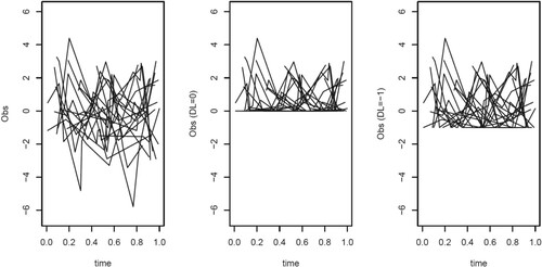
Figure 2. For replicate 1 of the sparse setting, contour plots with lines of the true and estimated covariance function for a DL of 0 (top layer) and of $-1$ (bottom layer) using the constant approximation methods with the OBS and SUBJ weighting schemes (second and third columns) and using PACE (fourth column). The covariance is estimated at 20 equal-distant points in $[0,1]\times [0,1]$. The bandwidth for the constant approximation method is 0.015.

For these two replicates, the proposed local constant approximation method performs much better than PACE. For $\mathrm{DL}=0$, PACE estimates the covariance of all considered time points larger than zero while the two local constant estimates also have negative values representing the true situation. For both values of DL, the OBS scheme seems to capture the true covariance function slightly better in this replicate. Further because of less missing values, the results for $\mathrm{DL}=-1$ (bottom layers of Figure 2) are better than that for $\mathrm{DL}=0$ (top layers of these figures). The time needed for calculating the estimate of the covariance function appeared to be 4.8 seconds for $\mathrm{DL}=-1$ and 5.1 seconds for $\mathrm{DL}=0$ for the proposed estimators while the computation time for the PACE method was 7.6 seconds for $\mathrm{DL}=-1$ and 7.9 seconds for $\mathrm{DL}=0$. Thus our proposed local approximation method is more time efficient than the PACE method.

For the dense setting, Figure 3 depicts the first 20 of the 100 trajectories in the first replicate without a DL and subject to a DL of $\mathrm{DL}=0$ and of $\mathrm{DL}=-1$. The proportions of observations subject to DL are 50.21% in the replicate with for $\mathrm{DL}=0$ and 25.61% for $\mathrm{DL}=-1$. The estimates of the covariance functions by the various methods using the data from these replicates are given in Figure 4.

Figure 3. The first 20 of the 100 trajectories in the first replicate of the dense setting. Left: Data without a detection limit, middle with a detection limit of 0, right with detection limit of $-1$.

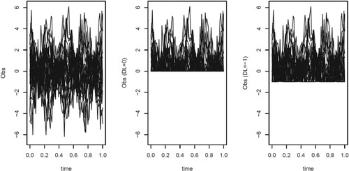
Figure 4. For replicate 1 of the dense setting, contour plots with lines of the true and estimated covariance function for a DL of 0 (top layer) and of $-1$ (bottom layer) using the constant approximation methods with the OBS and SUBJ weighting schemes (second and third columns) and using PACE (fourth column). The covariance is estimated at 20 equal-distant points in $[0,1]\times [0,1]$. The bandwidth for the constant approximation method is 0.03 for a DL of 0 and 0.035 for a DL of $-1$.

As in the sparse setting, the proposed local constant approximation method performs better than the existing PACE method for these two replicates. The two weighting schemes in the local constant approximation methods give similar estimates. The time needed for calculating the estimated covariance function is 0.03 seconds for $\mathrm{DL}=-1$ and 0.057 seconds for $\mathrm{DL}=0$ by using the local constant approximation, while for PACE it is 758 seconds for $\mathrm{DL}=-1$ and 773 seconds for $\mathrm{DL}=0$. Thus our proposed local approximation method is considerably more time efficient than the PACE method for the dense setting.

Table 1 shows the results of the simulation study based on all replicates. It provides the MISE and the corresponding standard deviation (SD) for local constant approximation for the two weighting schemes (SUBJ or OBS) for increasing sample size n. Also the mode of optimal bandwidth in local constant estimation selected for each replicate is provided. We did not show the results of the PACE method, as this method appeared to give biased and inaccurate estimates, see Figures 2 and 4.

Table 1. Results of the simulation study for the scenarios $\mathrm{DL}=0$ and $\mathrm{DL}=-1$ and for the sparse and dense setting.

	n = 100	n = 200	n = 500	n = 1000
	Dense (DL$=0$)
$\hat{C}$ (OBS)	0.348(0.147,0.015)	0.305(0.107,0.015)	0.295(0.096,0.015)	0.276(0.050,0.015)
$\hat{C}$ (SUBJ)	0.347(0.147,0.015)	0.306(0.107,0.015)	0.296(0.095,0.015)	0.276(0.049,0.015)
	Dense (DL$=-1$)
$\hat{C}$ (OBS)	0.145(0.120,0.015)	0.105(0.078,0.015)	0.099(0.076,0.015)	0.080(0.036,0.015)
$\hat{C}$ (SUBJ)	0.144(0.120,0.015)	0.107(0.078,0.015)	0.099(0.075,0.015)	0.080(0.035,0.015)
	Sparse (DL$=0$)
$\hat{C}$ (OBS)	1.080(0.307,0.030)	0.771(0.190,0.03)	0.598(0.114,0.03${}^{\ast }$)	0.538(0.080,0.03${}^{\ast }$)
$\hat{C}$ (SUBJ)	1.269(0.682,0.035)	0.881(0.199,0.03)	0.662(0.110,0.03${}^{\ast }$)	0.582(0.072,0.03${}^{\ast }$)
	Sparse (DL$=-1$)
$\hat{C}$ (OBS)	0.769(0.267,0.035)	0.501(0.137,0.03)	0.350(0.100,0.025${}^{\ast \ast }$)	0.249(0.070,0.025${}^{\ast \ast }$)
$\hat{C}$ (SUBJ)	0.918(0.401,0.035)	0.602(0.142,0.03)	0.421(0.100,0.025${}^{\ast \ast }$)	0.293(0.061,0.025${}^{\ast \ast }$)

Note: Reported are MISE (SD, mode of optimal bandwidth of local constant approximation), see formulas (5(5) $\begin{array}{rl}MISE(\hat{C}(s,t))& =\frac{1}{Q}\sum _{i=1}^{Q}IS{E}_{opt}({\hat{C}}^{([i])}(s,t)),\end{array}$(5) ) and (6(6) $\begin{array}{rl}SD(\hat{C}(s,t))& =\sqrt{\frac{1}{Q-1}\sum _{i=1}^Q{(IS{E}_{opt}({\hat{C}}^{([i])}(s,t))-MISE(\hat{C}(s,t)))}^2},\end{array}$(6) ) for the definition of MISE and SD respectively. n is the sample size (100, 200, 500 and 1000). The optimal bandwidth is selected based on the MISE criteria. The covariance function is estimated at 20 equal-distant time points in $[0,1]\times [0,1]$. The number of replicates is 100.${}^{\ast }$Bandwidth is fixed at 0.03, and the reason is the selected optimal bandwidths for cases n = 100 and n = 200 are all 0.03, and we expect for n = 500 and n = 500 bandwidth does not change much and this reduce the computation time a lot.${}^{\ast \ast }$Bandwidth is 0.025 or 0.03 selected based on MISE.

Clearly as n increases from 100 to 1000, the MISE and corresponding SD decreases. The dense case has smaller MISE compared to the sparse case. Comparing $\mathrm{DL}=-1$ with $\mathrm{DL}=0$, MISE is smaller for $\mathrm{DL}=-1$. This can be explained by the fact that there is more information for $\mathrm{DL}=-1$ and in the dense setting. The optimal bandwidth is very stable across all settings for both weighting schemes. For the sparse setting, the OBS scheme performs better than the SUBJ scheme. For the dense setting, the two weighting schemes perform similar.

4. Data application

We illustrate our method using data from a longitudinal biomarker study of scleroderma patients. Scleroderma is a heterogeneous disease where the course of the severity varies among patients. The study comprises 217 patients with hospital visits from 2010 to 2015. Typically, scleroderma patients visit the hospital every 6 months to check whether the disease has progressed. However, patients missed their appointments or their data were not recorded resulting in a sparse unbalanced dataset. The data were collected according to the ethically approved protocol for observational study HRA number 15/NE/0211.

In Liu and Houwing-Duistermaat (2022), the mean functions of two biomarkers subject to detection limits were estimated, namely aldose reductase (AR) and alpha fetoprotein (AF). The percentage of missing data for the AF marker is high, namely 75%, which led to uncertainty in the estimation of the mean function. The percentage of missing data due to the DL for AR is much lower namely 7.8% observations resulting in a more stable mean function. For the estimation of the covariance function we use the data on AR.

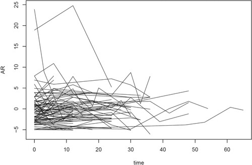
For data cleaning, we remove observations at time points with no outcomes or no biomarker values, and some outliers (AR has a value larger than 3 times the standard deviation). Finally, patients with only one observation are dropped. The final dataset comprises 90 patients within total 268 observations. The mean function of AR is estimated using the local constant approximation method under the OBS scheme. The bandwidth was selected using CV over a fine grid. The observed profiles minus the estimated mean function are shown in Figure 5.

Figure 5. The AR observations with estimated mean being subtracted.

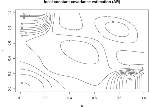
The estimate of the covariance function using the local constant method is shown in Figure 6. Note that the number of patients observed over a large time period is small, hence the covariance estimations for s or t larger than 0.6 have large uncertainty. For the region $[0,0.5]\times [\mathrm{0.0.5}],$ we observe that at larger distance the covariance decreases. Along the line s = t for the region $[0,0.5]\times [\mathrm{0.0.5}]$, the estimated covariance functions appear to decrease. This is probably due to a smaller variance (see Figure 5). Finally for the regions $[0.5,1]\times [\mathrm{0.0.5}]$ and $[0,0.5]\times [0.5,1]$, we observe that the covariance increases when s and t respectively increase to 1. This may reflect the fact that patients observed over a longer time range are a specific subset of the patients, namely they are more stable hence show a large correlation and a large covariance over time.

Figure 6. The covariance estimation for AR by using local constant estimation method.

5. Discussion

We have proposed a novel estimator for the covariance function for sparse and dense temporal data subject to a DL. Our method is based on local smoothing of the covariance function using kernel functions. We derived the asymptotic properties of the estimator and evaluated these properties via simulations. We compared our method to the method which ignores the presence of a DL in the data sample. We showed that our methods performed better in terms of bias and computation time. We also considered two weighting schemes for the observations, one based on single observations and one based on subjects. For sparse data, weighting per observation appeared to perform better.

We illustrated the method using data from a biomarker study. The estimated covariance for the biomarker first decreased over time and then started increasing again. The latter might be explained by an increase in variance and/or in correlation. If the biomarker represents disease severity, the patients who have a longer follow up are likely to be patients with a less severe disease course. Thus these results might be explained by non-random drop out of patients. The development of estimators for the mean and covariance function for drop out will be future research.

Liu and Houwing-Duistermaat (2022) also proposed a linear approximation instead of a constant approximation. We did not consider this approach here since for dense data there is no difference in performance and the linear approximation requires more computation time. For sparse data, a linear approximation might perform slightly better. Another approach is to impute the missing observations and then use PACE for the estimation of the covariance function. For cross-sectional data, Uh, Hartgers, Yazdanbakhsh, and Houwing-Duistermaat (2008) studied the performance of imputation methods. They concluded that these methods may give biased estimators or underestimated variances. Given the results of Uh et al. (2008) and the facts that multiple imputations would increase the computation time and that the computation time of PACE is higher than of our methods, we did not consider this approach for the estimation of covariance function.

For the selection of the bandwidth, we used cross validation in the data application while in the simulation we used ISE where we plug in the true value of the covariance function $C(t,s)$. We could have used cross validation in the simulation study as well, however, this would have increased the computation time while we expect that cross validation would only slightly change individual results and our overall conclusions with regard to the effect of DL on the estimation of the covariance and the difference between using OBS and SUBJ weighting would not change.

With the availability of estimators of the mean and the covariance function, models for temporal data subject to DL can be built. Functional principal component analysis (FPCA) can be used to reduce the infinite dimension into finite dimension. For sparse datasets, FPCA can be used to obtain smooth individual curves. Finally functional regression models can be developed to investigate the influence of covariates with DL on the outcomes which might be also subject to DL.

Acknowledgments

We would like to thank a referee for very useful constructive remarks.

Disclosure statement

No potential conflict of interest was reported by the author(s).

Additional information

Funding

This work is supported by a fellowship of the Alan Turing Institute, by Yujie Talent Project of North China University of Technology No. 107051360023XN075-04 and by the EU funded Cost action DYNALIFE, no CA21169.

Appendix

Notations

Notation B.1

Define the following notations:

• Coefficient functions $\begin{array}{rl}{w}_{i1}(s,t)& =[(-0.8194+0.502[-1,2]){\delta }_i(s)]\cdot [(-0.8194+0.502[-1,2]){\delta }_i(t)]\cdot v_i\\ w_{i2}(s,t)& =[1-0.498{\delta }_i(s)]\cdot [1-0.498{\delta }_i(t)]\cdot v_i\\ w_{i3}(s,t)& =[1-{\delta }_i(s)]\cdot [1-{\delta }_i(t)]\cdot v_i{w}_{i4}(s,t)\\ & =[(-0.8194+0.502[-1,2]){\delta }_i(s)]\cdot [1-0.498{\delta }_i(t)]\cdot v_i\end{array}$where $0.502[-1,2]$ means the interval $[-0.502,1.004]$ and therefore $w_{i1}(s,t)$ is a value in an closed interval for fixed s, t.

• Conditional expectations $\begin{array}{rl}{E}_0(s,t)& =E[Y_1{Y}_2|T_1=s,T_2=t]\\ E_1(s,t)& =E[Y_1{Y}_2{Y}_3|T_1=t,T_2=s,T_3=t]\\ E_2(s,t)& =E[Y_1^2{Y}_2|T_1=t,T_2=s]\\ E_3(s,t)& =E[Y_1{Y}_2{Y}_3{Y}_4|T_1=s,T_2=t,T_3=s,T_4=t]\\ E_4(s,t)& =E[Y_1^2{Y}_2{Y}_3|T_1=s,T_2=t,T_3=t]\\ E_5(s,t)& =E[Y_1^2{Y}_2^2|T_1=s,T_2=t].\end{array}$Note that since we assume in this section $\mu (t)=0$, for independent random variables $T_1$ and $T_2$, we denote $E_0(s,t)=E[Y_1{Y}_2|T_1=s,T_2=t]$; otherwise, $E_0(s,t)=E[(Y_1-\mu (T_1))(Y_2-\mu (T_2)|T_1=s,T_2=t]$. The other notations $E_i(s,t),i=1,2,\dots ,5$ are similar.

• Covariance functions $\begin{array}{rl}{V}_i^I(s,t)& =N_i(N_i-1)(1+I_{s=t})\frac{\Vert K{\Vert }^4}{h^2}(f(s)f(t)+o(1))\\ & +N_i(N_i-1)(N_i-2)(1+I_{s=t})\frac{\Vert K{\Vert }^2}{h}(f(s)f^2(t)+f^2(s)f(t)+o(1))\\ & +(N_i(N_i-1)(N_i-2)(N_i-3)-(N_i(N_i-1){)}^2)(f^2(s)f^2(t)+o(1)),\\ V_i^{II}(s,t)& =N_i(N_i-1)I_{s=t}\frac{\Vert K{\Vert }^4}{h^2}(f(s)f(t)E_0(t,t)+o(1))\\ & +N_i(N_i-1)(N_i-2)\frac{\Vert K{\Vert }^2}{h}(f^2(s)f(t)E_0(t,t)+o(1))\\ V_i^{III}(s,t)& =N_i(N_i-1)I_{s=t}\frac{\Vert K{\Vert }^4}{h^2}(f^2(s)E_0(s,t)+o(1))\\ & +N_i(N_i-1)(N_i-2)I_{s=t}\frac{\Vert K{\Vert }^2}{h}(f^3(s)E_0(s,t)+o(1))\\ V_i^{IV}(s,t)& =N_i(N_i-1)(1+I_{s=t})\frac{\Vert K{\Vert }^4}{h^2}(f(s)f(t)E_2(s,t)+o(1))\\ & +N_i(N_i-1)(N_i-2)(1+I_{s=t})\frac{\Vert K{\Vert }^2}{h}(f(s)f^2(t)E_1(s,t)+f^2(s)f(t)E_2(s,t)+o(1))\\ & +N_i(N_i-1)(N_i-2)(N_i-2)(f^2(s)f^2(t)+o(1))\\ V_i^V(s,t)& =N_i(N_i-1)(1+I_{s=t})\frac{\Vert K{\Vert }^4}{h^2}(f(s)f(t)E_5(s,t)+o(1))\\ & +N_i(N_i-1)(N_i-2)(1+I_{s=t})\frac{\Vert K{\Vert }^2}{h}(f(s)f^2(t)E_4(s,t)+f^2(s)f(t)E_4(t,s)+o(1))\\ & +N_i(N_i-1)(N_i-2)(N_i-2)(f^2(s)f^2(t)E_3(s,t)+o(1))\\ & -(N_i(N_i-1){)}^2{C}^2(s,t)(f^2(s)f^2(t)+o(1))\end{array}$

Assumptions

Assumption B.1

Assumptions for the Kernel function:

(A1)	Kernel function $K(\cdot )$ is a symmetric probability density function on $[-1,1]$, and ${\sigma }_K^2=\int u^{2}K(u)\mathrm{d}u<\mathrm{\infty }$and $\Vert K{\Vert }^2=\int K^2(u)\mathrm{d}u<\mathrm{\infty }.$

Assumption B.2

Assumptions for time points and the true functions:

(B1)	Time points $\{t_{ij},i=1,\dots ,n,j=1,\dots ,N_i\}$ are iid copies of a random variable T defined on interval I with density $f(\cdot )$: $0<m_f\le minf(t)\le maxf(t)\le M_f<\mathrm{\infty }$and $f^{{}^{″}}(t)$ is bounded.
(B2)	$X(t)$ is independent of T, ϵ is independent of T.
(B3)	$\frac{{\mathrm{\partial }}^{2}C(s,t)}{\mathrm{\partial }{s}^2},\frac{{\mathrm{\partial }}^{2}C(s,t)}{\mathrm{\partial }s\mathrm{\partial }s},\frac{{\mathrm{\partial }}^{2}C(s,t)}{\mathrm{\partial }{t}^2}$ are bounded on $I\times I$.

Assumption B.3

Assumptions for deriving the asymptotic distribution of the estimated covariance function:

(C1)	For $k_1,k_2=1,2,3,4$, as $n\to \mathrm{\infty }$, $\begin{array}{rl}& h:=h_n\to 0\\ & \frac{\sum _i{N}_i(N_i-1)w_{i{k}_1}(s,t)w_{i{k}_2}(s,t)}{h^2}\to 0\\ & \frac{\sum _i{N}_i(N_i-1)(N_i-2)w_{i{k}_1}(s,t)w_{i{k}_2}(s,t)}{h}\to 0\\ & \sum _i{N}_i(N_i-1)(N_i-2)(N_i-3)w_{i{k}_1}(s,t)w_{i{k}_2}(s,t)\to 0.\end{array}$
(C2)	For $k_1,k_2=1,2,3,4$, as $n\to \mathrm{\infty }$, $\begin{array}{rl}& \underset{k_1,k_2=1,2,3,4}{min}\{\frac{h^2}{\sum _i{N}_i(N_i-1)w_{i{k}_1}(s,t)w_{i{k}_2}(s,t)},\\ & \frac{h}{\sum _i{N}_i(N_i-1)(N_i-2)w_{i{k}_1}(s,t)w_{i{k}_2}(s,t)},\\ & \frac{1}{\sum _i{N}_i(N_i-1)(N_i-2)(N_i-3)w_{i{k}_1}(s,t)w_{i{k}_2}(s,t)}\}{h}^6\to 0.\end{array}$
(C3)	For $k_1,k_2,k_3=1,2,3,4$, as $n\to \mathrm{\infty }$, $\begin{array}{rl}& \underset{k_1,k_2,k_3=1,2,3,4}{max}\{\frac{\sum _i{N}_i(N_i-1)w_{i{k}_1}(s,t)w_{i{k}_2}{w}_{i{k}_3}(s,t)}{h^4},\\ & \frac{\sum _i{N}_i(N_i-1)(N_i-2)w_{i{k}_1}(s,t)w_{i{k}_2}{w}_{i{k}_3}(s,t)}{h^3},\\ & \frac{\sum _i{N}_i(N_i-1)(N_i-2)(N_i-3)w_{i{k}_1}(s,t)w_{i{k}_2}{w}_{i{k}_3}(s,t)}{h^2},\\ & \frac{\sum _i{N}_i(N_i-1)(N_i-2)(N_i-3)(N_i-4)w_{i{k}_1}(s,t)w_{i{k}_2}{w}_{i{k}_3}(s,t)}{h},\\ & \sum _i{N}_i(N_i-1)(N_i-2)(N_i-3)(N_i-4)(N_i-5)w_{i{k}_1}(s,t)w_{i{k}_2}{w}_{i{k}_3}(s,t)\}/\\ & (\frac{\sum _i{N}_i(N_i-1)w_{i{k}_1}(s,t)w_{i{k}_2}(s,t)}{h^2},\\ & \frac{\sum _i{N}_i(N_i-1)(N_i-2)w_{i{k}_1}(s,t)w_{i{k}_2}(s,t)}{h},\\ & {\sum _i{N}_i(N_i-1)(N_i-2)(N_i-3)w_{i{k}_1}(s,t)w_{i{k}_2}(s,t))}^{\frac{3}{2}}\to 0.\end{array}$

Proof of Theorem 2.1

Proof.

The calculation of the asymptotic bias of $\hat{C}(s,t)$, $\begin{array}{rl}E[S_{00}]& =[f(s)f(t)+\frac{h^2}{2}{\sigma }_K^2{B}_1(s,t)+o(h^2)]\sum N_i(N_i-1)w_{i2}(s,t)\\ E[R_{00}]& =[f(s)f(t)+\frac{h^2}{2}{\sigma }_K^2{B}_1(s,t)+o(h^2)]\sum N_i(N_i-1)w_{i1}(s,t){\sigma }^2\\ & +[C(s,t)f(s)f(t)+\frac{h^2}{2}{\sigma }_K^2{B}_2(s,t)+o(h^2)]\sum N_i(N_i-1)w_{i2}(s,t),\end{array}$where $\begin{array}{rl}{B}_1(s,t)& =f^{{}^{″}}(s)f(t)+f(s)f^{{}^{″}}(t)\\ B_2(s,t)& =C(s,t)f^{{}^{″}}(s)f(t)+C(s,t)f(s)f^{{}^{″}}(t)\\ & +\frac{2\mathrm{\partial }C}{\mathrm{\partial }s}{f}^{\mathrm{\prime }}(s)f(t)+\frac{2\mathrm{\partial }C}{\mathrm{\partial }t}f(s)f^{\mathrm{\prime }}(t)+\frac{{\mathrm{\partial }}^{2}C}{\mathrm{\partial }{s}^2}f(s)f(t)+\frac{{\mathrm{\partial }}^{2}C}{\mathrm{\partial }{t}^2}f(s)f(t)\\ & =C(s,t)B_1(s,t)\\ & +\frac{2\mathrm{\partial }C}{\mathrm{\partial }s}{f}^{\mathrm{\prime }}(s)f(t)+\frac{2\mathrm{\partial }C}{\mathrm{\partial }t}f(s)f^{\mathrm{\prime }}(t)+\frac{{\mathrm{\partial }}^{2}C}{\mathrm{\partial }{s}^2}f(s)f(t)+\frac{{\mathrm{\partial }}^{2}C}{\mathrm{\partial }{t}^2}f(s)f(t)\end{array}$and ${\sigma }_K^2=\int u^{2}K(u)\mathrm{d}u.$Therefore, by using the delta method, the asymptotic bias is $\begin{array}{rl}E[\hat{C}(s,t)]-C(s,t)& =\frac{E[R_{00}]}{E[S_{00}]}-C(s,t)\\ & =B(s,t){\sigma }^2+\frac{h^2}{2}D(s,t)+o(h^2).\end{array}$For the asymptotic variance, we need to calculate $var(S_{00}),var(R_{00}),cov(R_{00},S_{00})$. This involves the calculation of $E[K_h(T-s)K_h(T-t)]$ which is equal to $\frac{\Vert K{\Vert }^{2}f(t)}{h}+o(\frac{1}{h})$ if s = t and 0 if $s\ne t$ as $h\to 0$, because the support of $K(t)$ is $[-1,1]$. Thus $\begin{array}{rl}var(S_{00})& =\sum w_{i2}^2(s,t)V_i^I(s,t),\\ var(R_{00})& =\sum w_{i1}^2(s,t){\sigma }^4{V}_i^I(s,t)+2\sum w_{i1}(s,t)w_{i2}(s,t)C(s,t){\sigma }^2{V}_i^I(s,t)\\ & +\sum w_{i4}^2(s,t){\sigma }^2{V}_i^{II}(s,t)+2\sum w_{i4}(s,t)w_{i4}(t,s){\sigma }^2{V}_i^{III}(s,t)\\ & +2\sum w_{i2}(s,t)w_{i4}(s,t)\sigma V_i^{IV}(s,t)+\sum w_{i4}^2(t,s){\sigma }^2{V}_i^{II}(t,s)\\ & +2\sum w_{i2}(t,s)w_{i4}(t,s)\sigma V_i^{IV}(t,s)+\sum w_{i2}^2(s,t)V_i^V(s,t)\\ cov(R_{00},S_{00})& =\sum [w_{i2}^2(s,t)C(s,t)+w_{i1}(s,t)w_{i2}(s,t){\sigma }^2]V_i^I(s,t).\end{array}$Therefore, by using the delta method, the asymptotic variance is $\begin{array}{rl}var(\hat{C}(s,t))& ={\left(\begin{array}{c}{\displaystyle \frac{1}{E[S_{00}]}}\\ -{\displaystyle \frac{E[R_{00}]}{E[S_{00}^2]}}\end{array}\right)}^T\left(\begin{array}{cc}var(R_{00})& cov(R_{00},S_{00})\\ cov(R_{00},S_{00})& var(S_{00})\end{array}\right)\left(\begin{array}{c}{\displaystyle \frac{1}{E[S_{00}]}}\\ -{\displaystyle \frac{E[R_{00}]}{E[S_{00}^2]}}\end{array}\right)\\ & ={(\sum N_i(N_i-1)w_{i2}(s,t)f(s)f(t))}^{-2}\\ & \times [\sum (w_{i1}(s,t)-B(s,t)w_{i2}(s,t){)}^2{\sigma }^4{V}_i^I(s,t)\\ & +\sum w_{i4}^2(s,t){\sigma }^2{V}_i^{II}(s,t)+2\sum w_{i4}(s,t)w_{i4}(t,s){\sigma }^2{V}_i^{III}(s,t)\\ & +2\sum w_{i2}(s,t)w_{i4}(s,t)\sigma V_i^{IV}(s,t)+\sum w_{i4}^2(t,s){\sigma }^2{V}_i^{II}(t,s)\\ & +2\sum w_{i2}(t,s)w_{i4}(t,s)\sigma V_i^{IV}(t,s)+\sum w_{i2}^2(s,t)V_i^V(s,t)]\\ & ={\mathrm{\Gamma }}_{n,N_i}.\end{array}$

References

- Beran, J., and Liu, H. (2014), ‘On Estimation of Mean and Covariance Functions in Repeated Time Series with Long-memory Errors’, Lithuanian Mathematical Journal, 54(1), 8–34.
- Beran, J., and Liu, H. (2016), ‘Estimation of Eigenvalues, Eigenvectors and Scores in FDA Models with Strongly Dependent Errors’, Journal of Multivariate Analysis, 147, 218–233.
- Billingsley, P. (2008), Probability and Measure, Hoboken, New Jersey: John Wiley & Sons.
- Fan, J., and Gijbels, I. (1995), ‘Datadriven Bandwidth Selection in Local Polynomial Fitting: Variable Bandwidth and Spatial Adaptation’, Journal of the Royal Statistical Society: Series B (Methodological), 57(2), 371–394.
- Fan, J., and Gijbels, I. (2018), Local Polynomial Modelling and Its Applications: Monographs on Statistics and Applied Probability 66, London: Routledge.
- Ferraty, F., and Vieu, P. (2006), Nonparametric Functional Data Analysis: Theory and Practice, New York: Springer.
- Horváth, L., and Kokoszka, P. (2012), Inference for Functional Data with Applications, New York: Springer.
- Kokoszka, P., and Reimherr, M. (2017), Introduction to Functional Data Analysis, London: Chapman and Hall/CRC.
- Li, Y., and Hsing, T. (2010), ‘Uniform Convergence Rates for Nonparametric Regression and Principal Component Analysis in Functional/longitudinal Data’, The Annals of Statistics, 38(6), 3321–3351.
- Liu, H., and Houwing-Duistermaat, J. (2022), ‘Fast Estimators for the Mean Function for Functional Data with Detection Limits’, Stat, 11(1), e467.
- Peng, J., and Paul, D. (2009), ‘A Geometric Approach to Maximum Likelihood Estimation of the Functional Principal Components From Sparse Longitudinal Data’, Journal of Computational and Graphical Statistics, 18(4), 995–1015.
- Ramsay, J.O., and Silverman, B.W. (2005), Functional Data Analysis (2nd ed.), New York: Springer.
- Shao, J. (2003), Mathematical Statistics, New York: Springer Science & Business Media.
- Shi, H., Dong, J., Wang, L., and Cao, J. (2021), ‘Functional Principal Component Analysis for Longitudinal Data with Informative Dropout’, Statistics in Medicine, 40(3), 712–724.
- Uh, H.W., Hartgers, F.C., Yazdanbakhsh, M., and Houwing-Duistermaat, J.J. (2008), ‘Evaluation of Regression Methods When Immunological Measurements are Constrained by Detection Limits’, BMC Immunology, 9(1), 1–10.
- Wang, J.L., Chiou, J.M., and Müller, H.G. (2016), ‘Functional Data Analysis’, Annual Review of Statistics and Its Application, 3, 257–295.
- Yao, F., Müller, H.G., and Wang, J.L. (2005), ‘Functional Data Analysis for Sparse Longitudinal Data’, Journal of the American Statistical Association, 100(470), 577–590.
- Zhang, X., and Wang, J.L. (2016), ‘From Sparse to Dense Functional Data and Beyond’, The Annals of Statistics, 44(5), 2281–2321.