Integrated log-rank test

Abstract

The log-rank test can be viewed as nonparametric from the standpoint of a series of $2\times 2$ tables, as semi-parametric from the standpoint of the proportional hazards model and as parametric from the viewpoint of a constructed empirical process. Under non-proportional hazards the optimality afforded by this test is lost. Some of this lost power can be recovered by more carefully structured tests. We focus on the integrated log-rank test. Under certain alternatives, we show this test to be unbiased, and consistent. It will also be seen to correlate well with the uniformly most powerful test, a test that, in practice, is not available. The integrated log-rank test is a useful addition to the clinical researcher's toolbox. For the purposes of illustration we revisit 3 recently published large scale clinical trials.

Keywords:

• Area under curve
• Brownian motion
• delayed effects
• Donsker's theorem
• log-rank test

1. Introduction

In randomised clinical trials, interest will typically focus on the comparison of two survival curves, estimated using the Kaplan-Meier or Nelson-Aalen methods. In most cases the comparison concerns two parallel treatment arms although extensions to more than two groups are relatively straightforward. Our attention here is restricted to the case of two groups. In the light of its simplicity and optimality in proportional hazards situations, the log-rank test is by far the most commonly used test for comparing such estimated curves (Mantel 1966). Typically it will form the basis for sample size calculations when designing and analysing a large scale clinical trial. In the absence of any parametric assumptions on the conditional survival distributions, the log-rank test is known to yield maximum power under proportional hazards (PH) alternatives, that is, alternatives in which the hazard rates of the two groups is constant over time (Peto and Peto 1972). We describe this as a persistent treatment effect. Under non-proportional hazard situations this optimality is lost and indeed it is possible for the power of the log-rank test to be seriously compromised. Many observers have pointed this out and suggestions for alternatives when non-proportional hazards are anticipated have been made (Sposto and Stablein 1997; Klein et al. 2007; Logan et al. 2008; Lin and Leon 2017; O'Quigley 2022) and are well studied. While proportional hazards can be expressed in a relatively simple way, non-proportional hazards can manifest itself in a number of different ways.

Among these different ways, three of the most commonly encountered and the most easily understood are: (1) effects that diminish as time progresses, a commonly observed phenomenon in vaccine studies as well as studies where the reliability of a measured prognostic factor diminished through time, (2) effects that only manifest themselves after some initial period during which they appear to be absent, a commonly observed phenomenon in immunotherapy trials and (3) the so-called crossing survival curves problem in which effects initially appear to go in one direction but later in the study reverse and go in the opposite direction. This last situation is the least common but has been observed in studies involving surgery or studies on graft versus host disease where an initial disadvantage, if overcome, can show itself to be a long term advantage.

Fleming and Harrington (1991) have considered the $G^{\rho ,\gamma }$ family of test statistics providing a set of weighted log-rank statistics. While all choices will correctly control for type 1 error, different choices can result in greater or in reduced power. The choice $G^{0,0}$ specifies equal weights and corresponds to the log-rank test, $G^{1,0}$ places more weight on earlier time points whereas $G^{0,1}$ places more weight on the later time points. Then, $G^{1,0}$ is more sensitive to early difference, a situation that corresponds to diminishing treatment effect, while $G^{0,1}$ is more sensitive to late divergence of survival curves. Careful specification of the ρ and γ parameters can result in tests with very good power properties. Likewise, any misspecification can imply a loss of power. With this in mind, Lee (1996) investigates a versatile test including some particular cases of $G^{\rho ,\gamma },$ while other closely related flexible tests have also been studied (Wu and Gilbert 2002; Lee 2007).

More recent work has pushed these ideas further, investigating in particular performance of the so-called max-combo test in various situations (Lin et al. 2020; Wang et al. 2021). When treatment effects diminish through time or only manifest themselves after a significant delay, perhaps in a staggered fashion, then the log-rank test can potentially be seriously handicapped. The test may be unable to reproduce the hoped for power that would have been a part of our initial design calculations. This would naturally be the case when those initial power calculations make an appeal to an alternative characterised by a persistent treatment effect that remains steadily at its maximum. These calculations will roughly hold, albeit with some loss in power, when the treatment effect corresponds to some kind of average over the study period. The further this average from the steady anticipated maximum the greater the loss in power. Recently, a family of tests was developed for situations such as this and presents the potential for significant power gains in many circumstances (Chauvel and O'Quigley 2014; O'Quigley 2021). Our interest focuses on one particular member of this family, a test we refer to as the integrated log-rank test. One notable advantage of this particular test is that, while obtaining an important power advantage over the log-rank test in the presence of non-proportional hazards, the test loses relatively little when, indeed, the hazards are strictly proportional. Combining this test with the log-rank test is easily done and allows the possibility of getting the best of both worlds. The investigators can decide in advance how likely and by how much the real situation may stray from a proportional hazards one, enabling us to minimise potential power losses. An accurate evaluation of the real, unknown, situation is rewarded with very high, near optimal power. The trial designer can be comforted by such knowledge but might gain even greater comfort from knowing that an inaccurate evaluation, while losing optimality properties, may not be greatly penalised.

Our purpose here is to carry out further exploration of the tests based on the regression effect process with a particular focus on the integrated log-rank test, a test that relates closely to the AUC test but with a sequential standardisation that mirrors that of the log-rank construction. The test shows itself to perform especially well in particular settings, notably those where the treatment effect declines or increases monotonically through time. Under a null hypothesis of no effect, seen as a function of time, the integrated log-rank test will look like the area under a Brownian motion which, on average, will be zero. Note that area below the axis is counted as negative area. Brownian motion will look like the sum of a large number of zero mean random effects. Under a proportional hazards alternative, this regression effect process will look like Brownian motion with linear drift, the slope of this drift depending both on the sample size and the true strength of effect as measured by the regression coefficient. In a large sample sense, the log-rank test corresponds to Brownian motion whereas the integrated log-rank test corresponds to integrated Brownian motion.

The integrated log-rank test will correlate strongly with the distance travelled from the origin of the regression effect process when the hazards are proportional, this distance equating to the log-rank test. Of greater interest is the fact that the integrated log-rank test will continue to maintain good power in the presence of non-proportional hazards effects when the regression effect process has a monotonic albeit non-linear trend. We organise the article as follows. In Section 2, notation, model structure and the regression effect process in transformed time are described. Section 3 describes informally how the regression effect process opens the door to many families of tests including the log-rank and integrated log-rank tests. Section 4 pursues these ideas in a more formal statistical setting. Asymptotic theory is briefly considered in Section 5 while Section 6 presents results allowing us to gain insight on the relative efficiency of the integrated log-rank test alongside the log-rank test.

2. Basic methodology

The two subsections here outline the methods that we use. The first subsection summarises the notation and provides the essential definitions, following which we present the model structure and model parametrisation. The second subsection describes the regression effect process which is the basis for the tests that follow.

2.1. Notation and definitions

We make use of the indicator function ${\mathcal{I}}_A,$ taking the value 1 when A holds and 0 otherwise. We use an alternate notation, $\mathcal{I}(A)$ when A is too long or too crowded for easy reading. Thus, $\mathcal{I}(A)={\mathcal{I}}_A.$ We denote the cardinality of the set A by $\mathcal{C}(A)$ and, aside from some technical value in the context of large sample theory, this will simply be the number of elements in the set A. The random variables of interest are the failure time, $T_i$, the censoring time, $C_i,$ and the treatment indicator covariate, $Z_i$, $i=1,\dots ,n.$ Under weak assumptions (bounded, predictable process) we can allow $Z_i(t)$ to change with time, t. In most of the applications considered here the treatment indicator covariate, $Z_i$ will remain constant in time. We can view these variables as a random sample from the distribution of T, C and Z. For each subject i we observe $X_i=min(T_i,C_i)$, and ${\delta }_i={\mathcal{I}}_{T_i\le C_i}$. The ‘at risk’ indicator $Y_i(t)$ is defined as, $Y_i(t)={\mathcal{I}}_{(X_i\ge t)}.$ The counting process $N_i(t)$ is defined as, $N_i(t)={\mathcal{I}}_{\{T_i\le t,T_i\le C_i\}}$ and we also define $\overline{N}(t)=\sum _1^n{N}_i(t)$. An important quantity, the ‘effective sample size’, is $k_n$ where, $k_n=\sum _{i=1}^n{\delta }_i\times \mathrm{\Delta }(X_i)\text{and where}\mathrm{\Delta }(t)=\mathcal{I}\{\sum _i\sum _j(Z_j-Z_i{)}^2{\mathcal{I}}_{X_j\ge t}{\mathcal{I}}_{X_i\ge t}>0\},$which will only differ from zero when, at time t, there are in the risk set at least two subjects with distinct covariate values. For continuous covariates, and no ties, $k_n$ corresponds to the number of observed failures. For a discrete covariate, for example a binary group indicator, $k_n$ counts the number of failures that are informative regarding regression effects, i.e. failures $X_i$ for which $\mathrm{\Delta }(X_i)=1$. Once one group has been exhausted and the remaining failures occur in a single group, then no information can be provided regarding the regression effect and $\mathrm{\Delta }(X_i)=0.$ While this is no doubt obvious it is nonetheless a little awkward notationally but is required in the semi-parametric context of proportional hazards regression. Fully parametric models are a different story. Semi-parametric inference remains invariant under monotonic increasing transformation of the $X_i$. Chauvel and O'Quigley (2014) chose to work with a very specific transformation given by the following definition.

Definition 2.1

Consider the following transformation ${\varphi }_n$ of the observed times $X_1,\dots ,X_n$: ${\varphi }_n(X_i)=\frac{1}{k_n}[\overline{N}(X_i)+(1-{\delta }_i)\frac{\mathcal{C}\{j:j=1,\dots ,n,X_j<X_i,\overline{N}(X_j)=\overline{N}(X_i)\}}{\mathcal{C}\{j:j=1,\dots ,n,\overline{N}(X_j)=\overline{N}(X_i)\}}],$and set ${\varphi }_n(0)=0.$ We define the inverse ${\varphi }_n^{-1}$ of ${\varphi }_n$ on $[0,1]$ by ${\varphi }_n^{-1}(t)=inf\{X_i,{\varphi }_n(X_i)\ge t,i=1,\dots ,n\},0\le t\le 1.$

The transformation ${\varphi }_n(X_i)$ defines an isomorphism from the set of the observed times $X_1,\dots ,X_n$ to the set of equally spaced new ‘failure’ times, $t_i=i/k_n,i=1,\dots ,k_n,$ together with the censorings that are placed uniformly between the corresponding transformed failure times. To the new set we add $t_0=0.$ Recall that the counting process $\{\overline{N}(t){\}}_{t\in [0,\mathcal{T}]}$ has a jump of size 1 at each time of death. Thus, on the new time scale representing the image of the observed times $\{X_1,\dots ,X_n\}$ under ${\varphi }_n$, the values in the set $\{1/k_n,2/k_n,\dots ,1\}$ precisely correspond to times of death, and the ith time of death $t_i$ is such that $t_i=i/k_n,i=1,\dots ,k_n.$

The set $\{1/k_n,2/k_n,\dots ,1\}$ is included in but is not necessarily equal to the transformed set of times of death. Working with the first $k_n$ of these, we restrict ourselves to values less than or equal to 1. As the importance of the transformation applied to the observed times is to preserve order, various transformations – treating censoring times differently – could be used. We choose to uniformly distribute censoring times between adjacent times of failure. The time ${\tau }_0$ on this new scale corresponds to the $(100\times {\tau }_0)$th percentile for informative ($\mathrm{\Delta }(X_i)\ne 0$) deaths in the sample. For example, at time ${\tau }_0=0.5,$ half of these deaths have been observed. At time ${\tau }_0=0.2$, we can say that $20\mathrm{\%}$ of these deaths have occurred. The inverse of ${\varphi }_n$ can be obtained easily and with it we can interpret the results on the initial time scale. All of our workings will be on the transformed time scale in $[0,1]$ and, to make this clear, we express the analogous quantities to those presented above but with respect to the new time scale. Specifically, for $t\in [0,1]$, we define the individual at risk and counting processes, $Y_i^{\ast }(t)$ and $N_i^{\ast }(t)$ for individuals $i=1,\dots ,n,$ as well as the cumulative process by, $Y_i^{\ast }(t)={\mathcal{I}}_{{\varphi }_n(X_i)\ge t},N_i^{\ast }(t)={\mathcal{I}}_{{\varphi }_n(X_i)\le t,{\delta }_i=1},{\overline{N}}^{\ast }(t)=\sum _{i=1}^n{N}_i^{\ast }(t).$Finally, denote $\mathrm{\Phi }(.)$ the distribution function of the normed and centred normal distribution. If there are ties in the data our suggestion is to split them randomly although there are a number of other suggested ways of dealing with ties. All of the techniques described here require only superficial modification in order to accommodate any of these other approaches for dealing with ties.

2.2. Regression effect process in transformed time

Our main building blocks are the conditional means and variances of the covariate over the risk set at time t. Many works show how to derive these on the basis of the non-proportional hazards model, $\lambda (t|Z)={\lambda }_0(t)\exp \{\beta (t)Z\},$ or we could, instead, simply define them directly. This can be a little sharper and so we consider the following three definitions.

Definition 2.2

We denote $\mathcal{Z}=\{\mathcal{Z}(t),t\in [0,1]\}$ a process such that (1) $\mathcal{Z}(t)=\sum _{i=1}^n{Z}_i\left(X_i\right)\mathcal{I}\{{\varphi }_n(X_i)=t,{\delta }_i=1\},t\in [0,1].$(1)

In words, $\mathcal{Z}$ assumes the value of the covariate (group assignment) associated with the failure, when there is one, at time t, otherwise it assumes the value zero.

Definition 2.3

For $i=1,\dots ,n$ and $t\in [0,1],$ the probability that individual i dies at time t under the non-proportional hazards model with parameter $\beta (t)$, conditional on the set of individuals at risk at time of death t, is defined by ${\pi }_i(\beta (t),t)=\frac{Y_i^{\ast }(t)\exp (\beta (t)Z_i({\varphi }_n^{-1}(t))){\mathcal{I}}_{k_{n}t\in \mathbb{N}}}{\sum _{j=1}^n{Y}_j^{\ast }(t)\exp (\beta (t)Z_j({\varphi }_n^{-1}(t)))},.$

Remark

The only values at which these quantities will be calculated are the times of death $t_1,\dots ,t_{k_n}$. We nevertheless define $\mathcal{Z}(t)$ and $\{{\pi }_i(\beta (t),t),i=1,\dots ,n\}$ for all $t\in [0,1]$ in order to be able to write their respective sums as integrals with respect to the counting process ${\overline{N}}^{\ast }$. The values 0 taken by them at times other than that of death are chosen arbitrarily although bounded by adjacent failures, i.e. the initial ordering is respected.

Expectations and variances with respect to the family of probabilities $\{{\pi }_i(\beta (t),t),i=1,\dots ,n\}$ can now be defined.

Definition 2.4

Let $t\in [0,1]$. The time dependent expectations and variances of Z with respect to the family of probabilities $\{{\pi }_i(\beta (t),t),i=1,\dots ,n\}$ are obtained from the moments expressed on the transformed scale as: (2) ${\mathcal{E}}_{\beta (t)}(Z^m|t)=\sum _{i=1}^n{Z}_i^m({\varphi }_n^{-1}(t)){\pi }_i(\beta (t),t),m=1,2,\dots$(2) giving the expected values as ${\mathcal{E}}_{\beta (t)}(Z|t)$ and the variances, ${\mathcal{V}}_{\beta (t)}(Z|t)={\mathcal{E}}_{\beta (t)}(Z^2|t)-{\mathcal{E}}_{\beta (t)}^2(Z|t).$ Note that at any fixed $t,\beta (t)=\beta$ can be viewed as an argument to $\mathcal{E}$ and that $\frac{\mathrm{\partial }}{\mathrm{\partial }\beta }{\mathcal{E}}_{\beta }(Z|t)={\mathcal{V}}_{\beta }(Z|t)$, for $t\in [0,1]$.

Proposition 2.1

Let $t\in [0,1]$. Under the non-proportional hazards model with parameter $\beta (t)$, the expectation $E_{\beta (t)}(\mathcal{Z}(t)|{\mathcal{F}}_{t^{-}}^{\ast })$ and variance $V_{\beta (t)}(\mathcal{Z}(t)|{\mathcal{F}}_{t^{-}}^{\ast })$ of the random variable $\mathcal{Z}(t)$ given the σ-algebra ${\mathcal{F}}_{t^{-}}^{\ast }$ are $E_{\beta (t)}(\mathcal{Z}(t)|{\mathcal{F}}_{t^{-}}^{\ast })={\mathcal{E}}_{\beta (t)}(Z|t),V_{\beta (t)}(\mathcal{Z}(t)|{\mathcal{F}}_{t^{-}}^{\ast })={\mathcal{V}}_{\beta (t)}(Z|t).$

The proof of the proposition is given in Section 5. In conclusion, for $j=1,\dots ,k_n$ and time of death $t_j$, by conditioning on the set of at-risk individuals, the expectation of $\mathcal{Z}(t_j)$ is ${\mathcal{E}}_{\beta (t_j)}(Z|t_j)$ and its variance-covariance matrix is ${\mathcal{V}}_{\beta (t_j)}(Z|t_j)$. Knowledge of these moments allows us to deduce the large sample behaviour of the tests described in the following section.

Definition 2.5

The regression effect process, $U_n^{\ast }$ on $[0,1],$ is obtained by linearly interpolating the $k_n+1$ random variables $\{U_n^{\ast }(\beta (t_j),t_j),j=0,1,\dots ,k_n\},$ one of which is degenerate, taking on the value zero with probability one when $t_0=0.$ Given $\beta (t),$ for $j=0,\dots ,k_n$ and for $t\in [t_j,t_{j+1}[$, we have; (3) $U_n^{\ast }(\beta (t),t)=U_n^{\ast }(\beta (t_j),t_j)+(t{k}_n-j)\{U_n^{\ast }(\beta (t_{j+1}),t_{j+1})-U_n^{\ast }(\beta (t_j),t_j)\}.$(3) in which, for $t_j=j/k_n,$ we write, (4) $U_n^{\ast }(\beta (t_j),t_j)=\frac{1}{\sqrt{k_n}}{\int }_0^{t_j}{\mathcal{V}}_{\beta (s)}(Z|s{)}^{-1/2}\{\mathcal{Z}(s)-{\mathcal{E}}_{\beta (s)}(Z|s)\}\mathrm{d}{\overline{N}}^{\ast }(s).$(4)

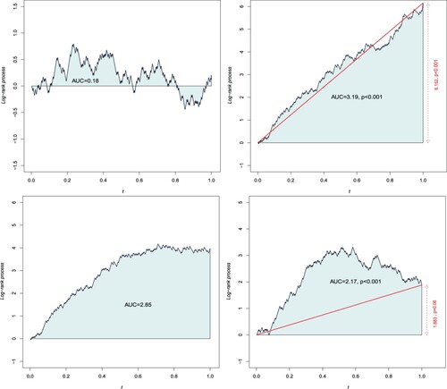
This process forms the basis for many statistical tests which are also accompanied by a simple visual representation of regression effects. Examples are seen in Figure 1. By virtue of Donsker-Prokhorov's invariance principle, $U_n^{\ast }(\beta (t),t)$ will look like Brownian motion when $\beta =0$ and Brownian motion with linear drift when $\beta ={\beta }_0\ne 0.$ The magnitude and sign of the drift will depend on the magnitude and sign of ${\beta }_0$ as well as $k_n.$

Figure 1. AUC for 4 situations with (a) no treatment effect $(\beta (t)=0)$; (b) $\beta (t)=0.5$; (c) $\beta (t)=0.5$ for t<0.5 and $\beta (t)=0$ for t>0.5; (d) $\beta (t)=0.5$ for t<0.5 and $\beta (t)=-0.25$ for $t>\mathrm{0.5.}$ Note that twice the area of the red triangle for the two right hand figures corresponds to the log-rank statistic.

3. Tests based on the regression effect process: general

A large number of tests can be based on the regression effect process. These include several well known families of tests such as the log-rank and weighted log-ranks tests. Our focus is on proportional hazards alternatives, alongside non-proportional hazards alternatives of a particular kind, specifically alternatives where the regression effect changes monotonically with time. For this purpose, we consider 5 classes of tests;

• Distance from the origin test.

• Log-rank test

• Area under the curve test

• Integrated log-rank test/conjugate integrated log-rank test

• Combined tests: log-rank/integrated log-rank tests and log-rank/conjugate integrated log-rank

The first 3 of these tests have been studied to a greater or lesser extent. The properties of the log-rank test are well known. Under proportional hazards alternatives, the distance from origin test is a uniformly most powerful test, a property inherited by the log-rank test under local alternatives. This follows from convergence in distribution results stemming from applications of the Donsker-Prokhorov invariance principle (Chauvel and O'Quigley 2014) and direct applications of the Neyman-Pearson lemma to the Brownian motion with linear drift law (Flandre and O'Quigley 2019). The area-under-the-curve test was introduced in O'Quigley (2008) and further studied by Chauvel and O'Quigley (2014). Here we focus on the test groupings based on the integrated log-rank test. We can deduce attractive properties for these tests by appealing to a convergence in distribution result showing, under certain conditions, the large sample equivalence of the area-under-the-curve test and the integrated log-rank test. Established Brownian motion theory also provides the large sample distribution for any linear combination of the log-rank and integrated log-rank test. The large sample correlation structure of the log-rank and the integrated log-rank test is a simple one so that tests that combine the log-rank with the integrated log-rank test are readily constructed. The test described in Section 3.3 is one such example and is of particular interest in that it mirrors the integrated log-rank test but with the weightings reversed, thereby providing improved power over the log-rank itself when regression effects increase, rather than decrease, with time. This test might be viewed as being based on the area over the curve and, in view of its particular relation to the integrated log-rank test, we call it the conjugate integrated log-rank test.

3.1. Distance-from-origin and log-rank tests

We briefly recall the idea behind the distance from origin test and how it relates to the log-rank test. The relationship between the area under the curve test and integrated log-rank test is then more easily understood. Figure 1 illustrates the connection between these tests and the regression effect process.

The ‘distance-from-origin at time t = 1 test’ – the $\text{DOT}(1)$ – test is the distance between the x-axis and the arrival point of the process when t = 1. Under proportional hazards the $\text{DOT}(1)$ test, i.e. $U_n^{\ast }(0,1)$ turns out to be the best available test (Chauvel and O'Quigley 2014), in the sense that it is the uniformly most powerful unbiased test over the domain of β. Consider though, when testing for the presence of an effect ($H_0:\beta (t)=0$ against $H_1:\beta (t)\ne 0$), and suppose that, instead of standardising by ${\mathcal{V}}_0(Z|t_i)$ at each $t_i$ we take a simple average of such quantities, over the observed failures. To see this, note that $\int {\mathcal{V}}_0(Z|t)\mathrm{d}\hat{F}(t)$ is consistent for $E\{\mathrm{Var}(Z|t)\}$ when $\beta (t)=0$, where $\hat{F}(t)$ is a consistent estimate of the distribution function of T, typically the Kaplan-Meier estimator. Rather than integrate with respect to $\hat{F}(t)$ it is more common, in the counting process context, to integrate with respect to $\overline{N}(t)$, the two coinciding in the absence of censoring. Either way, the approach amounts to averaging with respect to some empirical distribution. Now if, in the regression effect process, we replace ${\mathcal{V}}_{\beta }(Z|s)$ by ${\overline{\mathcal{V}}}_0(Z)$ then the statistic at $\mathrm{time}=1$, denoted by $L(1)$, coincides with the log-rank test. Noting that the distance from origin test is the uniformly most powerful unbiased test we might conclude that the log-rank test, as it stands, is generally a less powerful test. Such a conclusion is not incorrect but we need to be mindful of the fact that, for local alternatives, the two tests can be taken to be equivalent by virtue of a convergence in distribution result (Proposition 4.3).

We can say more. For non-local alternatives, the expected value (with respect to any distribution) of the distance from origin test is greater than or equal to that of the log-rank test. This follows by an application of Jensen's inequality showing that, for random variables A, where expectations exist, then $E(1/A)\ge 1/E(A).$ In theory then, we might hope the distance from the origin test to show some advantage over the log-rank test. In practice any advantage appears too small to make a difference and Proposition 4.3 indicates this difference to be zero for local alternatives. Inference for both tests as well as for the AUC test and integrated log-rank test lean on Theorem 1 below.

Figure 1 shows the results of a simulation of the process $U_n^{\ast }(0,t)$ describing situations with a sample size of 400 divided into two balanced treatment group (Z = 0 or 1). The first is absence of effect, i.e. under the null hypothesis $\beta (t)=0$, and this corresponds to Brownian motion (Figure 1(a)). The second situation describes a proportional hazards model with $\beta (t)=0.5$ (Figure 1(b)). This plot shows a linear trend from t = 0 to t = 1 corresponding to the value of β. The third situation corresponds to a simulated process under the non-proportional hazards model, with $\beta (t)$ taken to be piece-wise constant. Before t<0.5 there is a linear trend while for t>0.5 β equals zero and the process $U^{\ast }(0,t)$ is constant in expectation over time. The last situation corresponds also to a non-proportional hazards model with $\beta =0.5$ when t<0.5 and $\beta =-0.25$ when t>0.5 (Figure 1(d)). In this case, for t>0.5 the linear trend correspond to $\beta =-0.25$ and the survival curves crossed at the very end of the follow-up. The latter two situations correspond to the diminishing treatment effect issue.

3.2. Area-under-the-curve and integrated log-rank tests

A test of particular interest is that based on the area under the curve, $J({\beta }_0,t)={\int }_0^t{U}_n^{\ast }({\beta }_0,u)\mathrm{d}u.$ The area under the curve test is the area, positive and negative, between the process and the horizontal axis. Again, under the null hypothesis this has expectation equal to zero. Using standard results we have that $J({\beta }_0,t)$ converges in distribution to integrated Brownian motion, i.e. a Gaussian process with mean zero and covariance process (5) $\mathrm{Cov}\{J({\beta }_0,s),J({\beta }_0,t)\}=s^2(\frac{t}{2}-\frac{s}{6})(s<t).$(5) It is interesting to note that, unlike Brownian motion itself, integrated Brownian motion is not a martingale. At time t = 1, rather than base a test upon the distance covered by the process $U^{\ast }({\beta }_0,t)$ we can base a test upon the area under the curve. The two are correlated of course and if a large distance is covered we also know that there will be a large area under the curve. A two sided p-value corresponding to the null hypothesis is then obtained from $\text{Pr}\{\sqrt{3}|J({\beta }_0,t)/t\sqrt{t}|>z\}=2(1-\mathrm{\Phi }(z)).$Under departures from the null which can be exactly described as proportional hazards alternatives the distance from origin test has slightly greater power than the area under the curve test (Chauvel and O'Quigley 2014). This is no longer true when effects decline with time and in many, possibly the majority of practical situations the area under the curve test has greater power than the distance from origin test. The following theorem makes these observations more precise.

Theorem 3.1

Take $\mathbb{B}$ to be some set of continuous functions of t on $(0,1).$ Let ${\beta }_0\in \mathbb{B}$ be a constant function. Under the non-proportional hazards model with parameter $\beta (t)$, consider (6) $A_n(t)=\frac{1}{k_n}{\int }_0^t\{\beta (s)-{\beta }_0\}\frac{{\mathcal{V}}_{\tilde{\beta }(s)}(Z|s)}{{\mathcal{V}}_{{\beta }_0}(Z|s{)}^{1/2}}\mathrm{d}{\overline{N}}^{\ast }(s),0\le t\le 1,$(6) where $\tilde{\beta }$ is in the ball with centre β and radius $\underset{t\in [0,1]}{sup}|\beta (t)-{\beta }_0|$. Then, there exist two constants $C_1(\beta ,{\beta }_0)$ and $C_2\in {\mathbb{R}}^{\ast +}$ such that $C_1(\beta ,\beta )=1$ and (7) $U_n^{\ast }({\beta }_0,\cdot )-\sqrt{k_n}{A}_n\underset{n\to \mathrm{\infty }}{\overset{\mathcal{L}}{⟶}}{C}_1(\beta ,{\beta }_0)\mathcal{W}(t).$(7) where $\mathcal{W}(t)$ is a standard Brownian motion. Furthermore, (8) $\underset{0\le t\le 1}{sup}|A_n(t)-C_2{\int }_0^t\{\beta (s)-{\beta }_0\}\mathrm{d}s|\underset{n\to \mathrm{\infty }}{\overset{P}{⟶}}0.$(8)

Corollary 3.1

Under the non-proportional hazards model with parameter $\beta (t)$, $U_n^{\ast }(\beta (\cdot ),\cdot )\underset{n\to +\mathrm{\infty }}{\overset{\mathcal{L}}{⟶}}\mathcal{W}(t),$

Figure 1 gives a finite sample illustration of the implications of the theorem. A proof of the theorem is given in Chauvel and O'Quigley (2014). The implication of the theorem is that the regression effect process will trace out a path that closely parallels that of ${\int }_0^t\beta (u)du.$ Simulations back this up and it is straightforward to obtain curves such as those illustrated in the figure. On the original time scale however things will not look so clear cut so that, even in the case of proportional hazards, the process can appear to be non-linear.

3.3. Conjugate integrated log-rank test

The integrated log-rank test, in close agreement with the area under the curve test, will be sensitive to departures from the null in which treatment effects steadily wane with time. This is also the case for the $G^{p,0}$ class of tests. In a way not very dissimilar to the flipping of the $G^{1,0}$ test on its head to become the $G^{0,1}$ test, sensitive to treatment effects that increase rather than decrease in time, we can readily construct a test based on the integrated log-rank test that is also sensitive to treatment effects that increase with time. This construction is intimately related to the integrated log-rank test. So much so that we refer to it as the conjugate integrated log-rank test. Denoting the integrated log-rank test as $J({\beta }_0,t)$ then we refer to the conjugate integrated log-rank test as $J^{+}({\beta }_0,t)$ and we have: (9) $J^{+}({\beta }_0,t)+J({\beta }_0,t)=U_n^{\ast }({\beta }_0,t).$(9) so that, viewing $J({\beta }_0,t)$ as the area under the curve up until time point t, we can view $J^{+}({\beta }_0,t)$ as the area over the curve from the origin until time t. Figure 2 provides an illustration of where $J^{+}(0,1)$ can be used to advantage. We consider some of the details of large sample theory below but, already, we can see that working results are easily obtained since, under the hypothesis, $U_n^{\ast }({\beta }_0,t),$ $J({\beta }_0,t)$ and $J^{+}({\beta }_0,t)$ will be approximated by Gaussian processes with known means and known variance-covariance structure. In particular, to build a test based on the maximum of the log-rank and the conjugate integrated log-rank test, we can use the result; (10) $\mathrm{Cov}\{U_n^{\ast }({\beta }_0,t),J^{+}({\beta }_0,t)\}=\mathrm{Var}{U}_n^{\ast }({\beta }_0,t)-\mathrm{Cov}\{U_n^{\ast }({\beta }_0,t),J({\beta }_0,t)\}$(10) and this can be written down explicitly in terms of t.

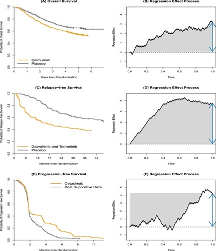
Figure 2. Figures (A) and (B) show effects that are approximately persistent. Here, twice the area under the curve and the log-rank statistic will be close and so we do not anticipate the integrated log-rank test to significantly outperform the log-rank test. Figures (C) and (D) show the strong erosion of effects that is not obvious from the K-M curves alone. The erosion is clear from the process (Figure D). Figures (E) and (F) indicate a delay in effects that is very sharp.

4. Tests based on the regression effect process: theory

The asymptotic behaviour of the regression effect process $U_n^{\ast }$ allows us to construct hypothesis tests on the value of the regression parameter $\beta (t)$. The null hypothesis $H_0$ and alternative hypothesis $H_1$ that we wish to test are $H_0:\mathrm{\forall }t,\beta (t)={\beta }_0,\mathrm{versus}{H}_1:{\displaystyle {\int }_{\mathcal{T}}\{\beta (t)-{\beta }_0{\}}^2\mathrm{d}t>0,}$where ${\beta }_0$ is a fixed constant and ${\int }_{\mathcal{T}}\mathrm{d}t>0.$ The reason for the slightly involved expression for $H_1$ is to overcome situations in which the test could be inconsistent. The expression allows us to cater for cases where, for example, $\beta (t)$ differs from ${\beta }_0$ only on a finite set of points or, to be more precise, on a set of time points of measure zero. Under $H_0$, the drift of the regression effect process $U_n^{\ast }({\beta }_0,\cdot )$ at ${\beta }_0$ is zero, and the process converges to standard Brownian motion. We can therefore base tests on the properties of Brownian motion. When ${\beta }_0=0$, this amounts to testing for the absence of an effect between the various values of the covariate Z. In particular, if the covariate is categorical and represents different treatment groups, this means testing the presence of a treatment effect on survival. The ${\beta }_0=0$ case corresponds to the null hypothesis of the log-rank test.

There are several possible tests based on the process, including the distance from the origin at time t, the maximal distance covered in a given time interval, the integral over some interval of the process, the supremum of a Brownian bridge, reflected Brownian motion and the arcsine law. We will take a closer look at how these relate to one another. We state a simple yet important proposition following which we look at the univariate case with one covariate and one effect to test (p = 1). Extensions to higher dimension are notationally but not theoretically demanding. For higher dimensions the number of processes of interest grows exponentially, for p = 2 for instance, we would have two conditional processes, two stratified processes, as well as processes arising as linear combinations. This is a potentially rich field for exploration and we do not take it any further here.

The following, almost trivial, result turns out to be of great help in our theoretical investigations. It is that every non-proportional hazard model, $\lambda (t|Z(t))={\lambda }_0(t)\exp \{\beta (t)Z(t)\}$, is equivalent to a proportional hazards model.

Lemma 4.1

For given $\beta (t)$ and covariate $Z(t)$ there exists a constant ${\beta }_0$ and time dependent covariate $Z^{\ast }(t)$ so that $\lambda (t|Z(t))={\lambda }_0(t)\exp \{\beta (t)Z(t)\}={\lambda }_0(t)\exp \{{\beta }_0{Z}^{\ast }(t)\}.$

There is no loss of generality if we take ${\beta }_0=1.$ The result is immediate upon introducing ${\beta }_0\ne 0$ and defining a time-dependent covariate $Z^{\ast }(t)\equiv Z(t)\beta (t){\beta }_0^{-1}.$ The important thing to note is that we have the same ${\lambda }_0(t)$ either side of the equation and that, whatever the value of $\lambda (t|Z(t))$, for all values of t, these values are exactly reproduced by either expression, i.e. we have equivalence. Simple though the lemma is, it has strong and important ramifications. It allows us to identify tests that are unbiased, consistent and, indeed, most powerful in given situations. A non-proportional hazards effect can thus be made equivalent to a proportional hazards one simply by multiplying the covariate Z by $\beta (t).$ The value of this may appear somewhat limited in that we do not know the form or magnitude of $\beta (t).$ However in terms of theoretical study, this simple observation is very useful. It will allow us to identify the uniformly most powerful test, generally unavailable to us in practice, and to gauge how close in performance comes any of those tests that are available. We first recall a useful result of Cox (1975). Under the non-proportional hazards model with $\beta (t)$, the increments of the process $U_n^{\ast }$ are centred with variance 1. From Proposition 4.1 we also have that these increments are uncorrelated, a key property in the derivation of the log-rank statistic.

Proposition 4.1

Cox 1975

Under the non-proportional hazards model with parameter $\beta (t)$, the increments between the random variables $U_n^{\ast }(\beta (t_j),t_j)$ and $U_n^{\ast }(\beta (t_{j-1}),t_{j-1})$ for $j=2,\dots ,k_n$ are uncorrelated.

Based on the regression effect process, two clear candidate statistics stand out for testing the null hypothesis of no effect. The first is the ‘distance-travelled’ at time t test and the second is the area under the curve test. Under proportional hazards the correlation between these two test statistics approaches one as we move away from the null. Even under the null this correlation is high and we consider this below. Under non-proportional hazards the two tests behave very differently. A combination of the two turns out to be particularly valuable for testing the null against various non-proportional hazards alternatives, including declining effects, delayed effects and effects that change direction during the study.

4.1. Distance travelled from the origin at time t

The distance travelled from the origin at time t, and in particular when $t=1,$ appears as a logical, and intuitive, candidate for a test. Much more can be said as we see in this section. Under the null, this distance, $U_n^{\ast }(0,1),$ has expectation equal to zero. The area under the curve test is the area, positive and negative, between the process and the time-axis. Again, under the null hypothesis this has expectation equal to zero. Under proportional hazards, the test based on $U_n^{\ast }(0,1)$ turns out to be the best available test for the following reasons.

Lemma 4.2

For 0<s<1 and under the null hypothesis, $H_0:\beta (t)=0,U_n^{\ast }(0,s)/\sqrt{s}$ converges in distribution to $\mathrm{\Phi }(z)$ where $\mathrm{\Phi }(\cdot )$ is the standard normal distribution.

Corollary 4.1

Set $z^{\alpha }$ such that $\alpha =2(1-\mathrm{\Phi }(z^{\alpha }))$. The distance travelled at time t test rejects $H_0$ with a type I error α if $|U^{\ast }({\beta }_0,t)/\sqrt{t}|\ge z^{\alpha /2}.$ The p-value for this test is given by $2[1-\mathrm{\Phi }(|U^{\ast }({\beta }_0,t)|/\sqrt{t})]$.

Corollary 4.2

The distance travelled test is unbiased against proportional hazards alternatives on the interval $(0,t)$.

Corollary 4.3

Under the null hypothesis, $H_0:\beta (t)=0,$ the distance travelled test is consistent against proportional hazards alternatives.

The lemma is an immediate consequence of the Donsker-Prokhorov invariance principle. The corollaries follow from the Neyman-Pearson lemma as applied to the standard normal distribution and one with the same variance but a translated mean.

Corollary 4.4

Under $H_1:\beta >0$, assuming the Breslow-Crowley conditions, i.e. $k_n/n\to \text{C}$ as $n\to \mathrm{\infty },$ then, for t>s $\underset{n\to \mathrm{\infty }}{lim}E{U}_n^{\ast }(0,t)-E{U}_n^{\ast }(0,s)=\mathcal{R}(k_n,\beta )(t-s),\underset{n\to \mathrm{\infty }}{lim}\mathrm{Var}\{U_n^{\ast }(0,t)-U_n^{\ast }(0,s)\}=t-s$where $\mathcal{R}$ behaves as a linear function of $k_n$ for fixed β and a linear function of β for fixed $k_n.$ Note that this function is not bounded with respect to increases in β and $k_n.$

Corollary 4.5

Under $H_1:\beta >0$, suppose that $\mathbb{P}(s)$ is the p-value for $U_n^{\ast }(0,s)/\sqrt{s},$ then, assuming that $k_n/n\to \text{C as}n\to \mathrm{\infty }$, then, for $t>s,E\mathbb{P}(t)<E\mathbb{P}(s).$

By applying the Neyman-Pearson lemma to the normal distribution, the above two corollaries tell us that the distance travelled test is the uniformly most powerful test of the null hypothesis, $H_0:\beta =0$ against the alternative, $H_1:\beta >0.$ The log-rank test, $L_n$ shares this property and this is formalised in Proposition 4.3. Lemma 4.1 allows us to make a stronger conclusion. Assume the non-proportional hazards model and consider the null hypothesis, $H_0:\beta (t)=0$ for all t. Then,

Lemma 4.3

The uniformly most powerful test of $H_0:\beta (t)=0$ for all t, is the distance travelled test applied to the proportional hazards model $\lambda (t|Z(t))={\lambda }_0(t)\exp \{{\beta }_0{Z}^{\ast }(t)\}$ in which $Z^{\ast }(t)={\beta }_0^{-1}\beta (t)Z(t)$ and where we take 0/0 to be equal to 1.

Since, under the alternative, we may have no information on the size or shape of $\beta (t),$ this result is not of any immediate practical value. It can though act as a bound, not unlike the Cramer-Rao bound for unbiased estimators and let us judge how well any test is performing when compared with the optimal test in that situation.

The following proposition states that the distance test statistic is consistent; that is, the larger the sample, the better we will be able to detect the alternative hypothesis of a proportional hazards nature. The result continues to hold for tests of the null versus non-proportional hazards alternatives but restrictions are needed, the most common one being that any non-null effect is monotonic through time.

Proposition 4.2

Under the alternative hypothesis $H_1:\beta (t)\ne {\beta }_0$, that is, under the non-proportional hazards model with parameter $\beta (t)\ne {\beta }_0$, we have $\underset{n\to \mathrm{\infty }}{lim}P(\frac{1}{\sqrt{t}}|U_n^{\ast }({\beta }_0,t)|\ge z^{\alpha /2})=1.$

Remark

The test can be applied at any time point t, making it flexible. For example, if we have prior knowledge that the effect disappears beyond some time point τ, we can apply the test over the time interval $(0,\tau )$. When such information is not available, we take t = 1, which, under proportional hazards, will maximise the power.

4.2. Relation between log-rank test and distance travelled test

Instead of standardising by ${\mathcal{V}}_0(Z|t_i)$ at each $t_i$ we might, instead, use a simple average of such quantities over the observed failures. Note that $\int {\mathcal{V}}_0(Z|t)\mathrm{d}\hat{F}(t)$ is consistent for $E(\mathrm{var}(Z|t))$ under the proportional hazards model with $\beta (t)=0$. Rather than integrate with respect to $d\hat{F}$ it is more common, in the counting process context, to integrate with respect to $d\overline{N}$, the two coinciding in the absence of censoring. If, we replace ${\mathcal{V}}_0(Z|s)$ by ${\overline{\mathcal{V}}}_0(Z)$ then the distance travelled test coincides exactly with the log-rank test. The following proposition gives an asymptotic equivalence under the null between the log-rank and the distance travelled tests:

Proposition 4.3

Chauvel and O'Quigley 2014

Let $L_n$ denote the log-rank statistic and let $U_n^{\ast }(0,1)$ be the distance statistic $U_n^{\ast }({\beta }_0,1)$ evaluated at ${\beta }_0=0$. We have that $|U_n^{\ast }(0,1)-L_n|\underset{n\to \mathrm{\infty }}{\overset{P}{⟶}}0.$

In order to obtain the result, we consider an asymptotic decomposition of the statistic $L_n$ in a Brownian motion with an added drift. The decomposition parallels that of the regression effect process at time t = 1. The conclusion is then immediate. A convergence in probability result implies a convergence in distribution result so that, under the conditions, the log-rank test and the distance from the origin test can be considered to be equivalent, this equivalence holding under the null and under local alternatives.

Under the conditions we have stated, the distance test statistic converges in distribution to that of the log-rank, guaranteeing maximum power under alternative hypotheses of the proportional hazards type. This result is not surprising since the expressions for the log-rank statistic $L_n$ and the distance test differ only in the standardisation used. For the former, standardisation takes place globally for all times at the end of the experiment, while for the latter, standardisation happens at each time of death. However, under a condition that holds precisely under the null and approximately under the alternatives, a condition analogous to that of homoscedasticity for the linear model (Chauvel and O'Quigley 2014), the standardisation does not change in expectation over time. Recall that this condition has been used by other authors (Grambsch and Therneau 1994). The result given in Proposition 4.3 also implies that the distance test is not optimal under alternative hypotheses of a non-proportional hazards nature since the power properties of the log-rank test also hold here. However, many other tests can be based on the regression effect process $U_n^{\ast }(t),$ the Donsker-Prokhorov invariance principle, and known properties of Brownian motion.

4.3. Combined log-rank and integrated log-rank tests

In the regression effect process, we might replace ${\mathcal{V}}_0(Z|t_i)$ at each time point $t_i$ by an average, ${\overline{\mathcal{V}}}_0(Z)=\int {\mathcal{V}}_0(Z|t)\mathrm{d}\hat{F}(t).$ While $\int {\mathcal{V}}_0(Z|t)\mathrm{d}\hat{F}(t)$ is not a martingale, it is consistent for $E(\mathrm{Var}(Z|t))$ under the proportional hazards model with $\beta (t)=0,$ so that, conditioning on the observed empirical variance allows us to treat this term as a constant. A similar argument has been used to justify the form of the log-rank test. Under the null, the conditional expectation does not depend on time, allowing us to work with ${\overline{\mathcal{V}}}_0(Z)$ instead of ${\mathcal{V}}_0(Z|s).$ In this way we can obtain a convergence in distribution result for $J_n(t)={\int }_0^t{U}_n^{\ast }(0,s)\mathrm{d}s$ and the area under the curve statistic, analogous to that of Proposition 4.3 above. More details are given in Section 5. The combined test, at $t=1,$ $M_{\theta }(1)$ where, $M_{\theta }(t)=\theta \times U_n^{\ast }(0,t)+(1-\theta )\times J_n(t),0\le \theta \le 1,$allows us to carry out a certain degree of fine tuning of the log-rank and integrated log-rank tests. When $\theta =1,$ $M_{\theta }(t)$ corresponds to the log-rank statistic whereas when $\theta =0,$ it equates to the integrated log-rank statistic. We see that $M_{\theta }(t)$ converges in distribution to a Gaussian process with mean zero and variance process equal to: (11) $t\times {\theta }^2+t^3\times (1-\theta {)}^2/3+t^2\times \theta (1-\theta ).$(11) which simplifies to $\{\theta (\theta -1)+1\}/3$ when $t=1.$ More generally we have;

Lemma 4.4

For time points s and t where $s<t,$ we can write; $\mathrm{Cov}\{M_{\theta }(s),M_{\theta }(t)\}={\theta }^{2}s+(1-\theta {)}^2{s}^2(\frac{t}{2}-\frac{s}{6})+\theta (1-\theta )s^2,$

noting that, as t approaches s from above, the expressions for the covariance and variance coincide. Mostly our interest will be on a single time point, often $t=1,$ so we will have little use for the covariance process. However, we can conceive of applications, such as clinical trials with interim analyses, where we may focus our interest on more than one time point. Although calculations may be fastidious there are no conceptual difficulties. With several time points, by virtue of having a Gaussian process, we can obtain all the needed terms of the required variance-covariance matrix.

Of equal interest, is a study on the pair $M_{{\theta }_1}(t)$ and $M_{{\theta }_2}(t)$ where ${\theta }_1\ne {\theta }_2.$ This could open the way to a further degree of combination or as a means to contrast different tests based on different weightings. Choosing ${\theta }_1={\theta }_2=1,$ allows for a study of the log-rank and integrated log-rank and these results we already have. But, of course, the comparison of other weightings can also be of interest. A calculation of the variances and co-variances allows us to obtain, for example, the Pitman efficiency of competing combinations. We have:

Lemma 4.5

At time t, for different values of the weighting parameter θ: $\mathrm{Cov}\{M_{{\theta }_1}(t),M_{{\theta }_2}(t)\}={\theta }_1{\theta }_{2}t+(1-{\theta }_1)(1-{\theta }_2)\frac{t^3}{3}+\{{\theta }_1(1-{\theta }_2)+{\theta }_2(1-{\theta }_1)\}\frac{t^2}{2}$

Lemma 4.4 provides the needed tool to study the process $M_{\theta }(t)$ in time while Lemma 4.5 allows us to study the impact of different weightings. It would be relatively straightforward to complete the picture by calculating the covariance process in time for different weightings but it is not easy to see any immediate applications for that. Combinations other than the simple linear one may also suggest themselves, one obvious candidate being the maximum of the two test statistics.

4.4. Kolmogorov type tests

Since we are viewing the process $U_n^{\ast }(\beta ,t)$ as though it were a realisation of a Brownian motion, we can consider some other well-known functions of Brownian motion. Consider then the bridged process $U_n^0(\beta (t),t)$;

Definition 4.1

The bridged process is defined by the transformation (12) $U_n^0(\beta (t),t)=U_n^{\ast }(\beta (t),t)-t\times U_n^{\ast }(\beta (t),1)$(12)

Lemma 4.6

The process $U_n^0(\beta (t),t)$ converges in distribution to the Brownian bridge, in particular $E{U}_n^0(\beta (t),t)=0$ and $\mathrm{Cov}\{U_n^0(\beta (t),s)$, $U_n^0(\beta (t),t)\}$ $=s(1-t).$

Note that a straightforward application of Slutsky's theorem enables us to claim that these large sample properties continue to hold whenever we use a consistent estimate in place of $\beta (t).$ In practice this would require us to limit $\beta (t)$ to a constant or a piecewise constant function of t.

The Brownian bridge is also called tied-down Brownian motion for the obvious reason that at t = 0 and t = 1 the process takes the value 0. Carrying out a test at t = 1 will not then be particularly useful and it is more useful to consider, as a test statistic, the greatest distance of the bridged process from the time axis. We can then appeal to:

Lemma 4.7

(13) $\mathrm{Pr}\{\underset{u}{sup}|U_n^0(\hat{\beta }(t),u)|\ge a\}\approx 2\exp (-2a^2),$(13)

which follows as a large sample result since $Pr\{\underset{u}{sup}|U_n^0(\hat{\beta }(t),u)|\le a\}\to 1-2\sum _{k=1}^{\mathrm{\infty }}(-1{)}^{k+1}\exp (-2k^2{a}^2),a\ge 0.$This is an alternating sign series and therefore, if we stop the series at k = 2 then the error is bounded by $2\exp (-8a^2)$ which for most values of a that we will be interested in will be small enough to ignore. For alternatives to the null hypothesis ($\beta =0$) belonging to the proportional hazards class, the Brownian bridge test is not generally a consistent test. The reason for this is that the transformation to the Brownian bridge will have the effect of cancelling the linear drift term. The large sample distribution under both the null and the alternative will be the same. Nonetheless, the test has value under alternatives of a non-proportional hazards nature, in particular an alternative in which $U_n^{\ast }(0,1)$ is close to zero, a situation we might anticipate when the hazard functions cross over. If the transformation to a Brownian bridge results in a process that would arise with small probability under the assumption of a Brownian bridge then this is indicative of effects of a non-proportional hazards nature.

5. Large sample approximations

Each time of death $t_i$ is a $({\mathcal{F}}_t^{\ast }{)}_{t\in [0,1]}$-stopping time where, for $t\in [0,1]$, the σ-algebra ${\mathcal{F}}_t^{\ast }$ is defined by ${\mathcal{F}}_t^{\ast }=\sigma \{N_i^{\ast }(u),Y_i^{\ast }(u^{+}),Z_i;i=1,\dots ,n;u=0,1,\dots ,\lfloor t{k}_n\rfloor \},$where $\lfloor \cdot \rfloor$ is the floor function and $Y_i^{\ast }(t^{+})=\underset{s\to t^{+}}{lim}{Y}_i^{\ast }(s)$. Notice that if $0\le s<t\le 1,$ ${\mathcal{F}}_s^{\ast }\subset {\mathcal{F}}_t^{\ast }$.

Remark

Denote $a\wedge b=min(a,b),$ for $a,b\in \mathbb{R}$. If the covariates are time-dependent, for $t\in [0,1]$, the σ-algebra ${\mathcal{F}}_t^{\ast }$ is defined by ${\mathcal{F}}_t^{\ast }=\sigma \{N_i^{\ast }(u),Y_i^{\ast }(u^{+}),Z_i({\varphi }_n^{-1}{\left(\frac{u}{k_n}\right)}^{+}\wedge X_i);i=1,\dots ,n;u=0,1,\dots ,\lfloor t{k}_n\rfloor \}$since, as we recall, the covariate $Z_i(\cdot )$ is not observed after time $X_i$, $i=1,\dots ,n$. To simplify notation in the following, we will write $Z_i({\varphi }_n^{-1}(t))$ in the place of $Z_i({\varphi }_n^{-1}(t{)}^{+}\wedge X_i),$, $t\in [0,1].$

In other words, ${\overline{N}}^{\ast }$ has jumps at times $t_j=j/k_n$ for $j=1,\dots ,k_n$. We make use of this in the following two lemmas.

Lemma 5.1

Let $n\in \mathbb{N}$ and let $\{A_n(t),t\in \{t_1,\dots ,t_{k_n}\}\}$ be a process with values in $\mathbb{R}$. Suppose that $\underset{i=1,\dots ,k_n}{sup}|A_n(t_i)-a(t_i)|\underset{n\to \mathrm{\infty }}{\overset{P}{⟶}}0,$where a is a function defined and bounded on $[0,1]$. Then, $\underset{s\in [0,1]}{sup}|\frac{1}{k_n}{\int }_0^s{A}_n(t)\mathrm{d}{\overline{N}}^{\ast }(t)-{\int }_0^{s}a(t)\mathrm{d}t|\underset{n\to \mathrm{\infty }}{\overset{P}{⟶}}0.$

Suppose that $\epsilon >0$. Note that (14) $\begin{array}{rl}& P\{\underset{0\le s\le 1}{sup}|\frac{1}{k_n}{\int }_0^s{A}_n(t)\mathrm{d}{\overline{N}}^{\ast }(t)-{\int }_0^{s}a(t)\mathrm{d}t|>\epsilon \}\\ & \le P\{\underset{0\le s\le 1}{sup}\frac{1}{k_n}|{\int }_0^s\{A_n(t)-a(t)\}\mathrm{d}{\overline{N}}^{\ast }(t)|>\frac{\epsilon }{2}\}\\ & +P\{\underset{0\le s\le 1}{sup}|\frac{1}{k_n}{\int }_0^{s}a(t)\mathrm{d}{\overline{N}}^{\ast }(t)-{\int }_0^{s}a(t)\mathrm{d}t|>\frac{\epsilon }{2}\}\end{array}$(14) Suppose also that $s\in [0,1].$ For the first term we have, $\begin{array}{rl}& \frac{1}{k_n}|{\int }_0^s\{A_n(t)-a(t)\}\mathrm{d}{\overline{N}}^{\ast }(t)|=\frac{1}{k_n}\left|\sum _{i=1}^{\lfloor k_{n}s\rfloor }(A_n(t_i)-a(t_i))\right|\\ & \le \frac{\lfloor k_{n}s\rfloor }{k_n}\underset{i=1,\dots ,\lfloor k_{n}s\rfloor }{sup}|A_n(t_i)-a(t_i)|\le \underset{i=1,\dots ,k_n}{sup}|A_n(t_i)-a(t_i)|.\end{array}$Therefore, $\underset{0\le s\le 1}{sup}\frac{1}{k_n}|{\int }_0^s\{A_n(t)-a(t)\}\mathrm{d}{\overline{N}}^{\ast }(t)|\le \underset{i=1,\dots ,k_n}{sup}|A_n(t_i)-a(t_i)|,$and $\underset{i=1,\dots ,k_n}{sup}|A_n(t_i)-a(t_i)|\underset{n\to \mathrm{\infty }}{\overset{P}{⟶}}0.$ As a result, $\underset{n\to \mathrm{\infty }}{lim}P\{\underset{0\le s\le 1}{sup}\frac{1}{k_n}|{\int }_0^s\{A_n(t)-a(t)\}\mathrm{d}{\overline{N}}^{\ast }(t)|>\frac{\epsilon }{2}\}=0.$For the second term on the right hand side of Equation (14(14) $\begin{array}{rl}& P\{\underset{0\le s\le 1}{sup}|\frac{1}{k_n}{\int }_0^s{A}_n(t)\mathrm{d}{\overline{N}}^{\ast }(t)-{\int }_0^{s}a(t)\mathrm{d}t|>\epsilon \}\\ & \le P\{\underset{0\le s\le 1}{sup}\frac{1}{k_n}|{\int }_0^s\{A_n(t)-a(t)\}\mathrm{d}{\overline{N}}^{\ast }(t)|>\frac{\epsilon }{2}\}\\ & +P\{\underset{0\le s\le 1}{sup}|\frac{1}{k_n}{\int }_0^{s}a(t)\mathrm{d}{\overline{N}}^{\ast }(t)-{\int }_0^{s}a(t)\mathrm{d}t|>\frac{\epsilon }{2}\}\end{array}$(14) ) we have, $\underset{0\le s\le 1}{sup}|\frac{1}{k_n}{\int }_0^{s}a(t)\mathrm{d}{\overline{N}}^{\ast }(t)-{\int }_0^{s}a(t)\mathrm{d}t|=\underset{0\le s\le 1}{sup}|\frac{1}{k_n}\sum _{i=1}^{\lfloor k_{n}s\rfloor }a\left(t_i\right)-{\int }_0^{s}a(t)\mathrm{d}t|.$Note that $a_n$ is piecewise constant on the interval $[0,1]$ such that $a_n(t)=a(t_i)$ for $t\in [t_i,t_{i+1}[$, $i=0,\dots ,k_n$. We then have, $\frac{1}{k_n}\sum _{i=1}^{\lfloor k_{n}s\rfloor }a\left(t_i\right)={\int }_0^s{a}_n(t)\mathrm{d}t-(s-\frac{\lfloor k_{n}s\rfloor }{k_n})a\left(\frac{\lfloor k_{n}s\rfloor }{k_n}\right).$As a result we have, $\begin{array}{rl}& \underset{0\le s\le 1}{sup}|\frac{1}{k_n}{\int }_0^{s}a(t)\mathrm{d}{\overline{N}}^{\ast }(t)-{\int }_0^{s}a(t)\mathrm{d}t|\\ & \le \underset{0\le s\le 1}{sup}|{\int }_0^s{a}_n(t)\mathrm{d}t-{\int }_0^{s}a(t)\mathrm{d}t|+\underset{0\le s\le 1}{sup}\left|(s-\frac{\lfloor k_{n}s\rfloor }{k_n})a\left(\frac{\lfloor k_{n}s\rfloor }{k_n}\right)\right|\\ & \le \underset{0\le s\le 1}{sup}|{\int }_0^s{a}_n(t)\mathrm{d}t-{\int }_0^{s}a(t)\mathrm{d}t|+\frac{1}{k_n}\underset{0\le s\le 1}{sup}\left|a\left(\frac{\lfloor k_{n}s\rfloor }{k_n}\right)\right|,\end{array}$Note that $\underset{n\to \mathrm{\infty }}{lim}\underset{s\in [0,1]}{sup}|a_n(s)-a(s)|=0$ by the uniform continuity of the function a. This implies uniform convergence $\underset{n\to \mathrm{\infty }}{lim}\underset{s\in [0,1]}{sup}|{\int }_0^s{a}_n(t)\mathrm{d}t-{\int }_0^{s}a(t)\mathrm{d}t|=0.$Furthermore, a is bounded so that $\underset{0\le s\le 1}{sup}|a(\frac{\lfloor k_{n}s\rfloor }{k_n})|<\mathrm{\infty },$ which shows the result since: (15) $\underset{n\to \mathrm{\infty }}{lim}\underset{0\le s\le 1}{sup}|\frac{1}{k_n}{\int }_0^{s}a(t)\mathrm{d}{\overline{N}}^{\ast }(t)-{\int }_0^{s}a(t)\mathrm{d}t|=0,$(15) Each time of death $t_i$ is a $({\mathcal{F}}_t^{\ast }{)}_{t\in [0,1]}$-stopping time where, for $t\in [0,1]$, the σ-algebra ${\mathcal{F}}_t^{\ast }$ is defined by ${\mathcal{F}}_t^{\ast }=\sigma \{N_i^{\ast }(u),Y_i^{\ast }(u^{+}),Z_i;i=1,\dots ,n;u=0,1,\dots ,\lfloor t{k}_n\rfloor \},$where $\lfloor \cdot \rfloor$ is the floor function and $Y_i^{\ast }(t^{+})=\underset{s\to t^{+}}{lim}{Y}_i^{\ast }(s)$. Notice that if $0\le s<t\le 1,$ ${\mathcal{F}}_s^{\ast }\subset {\mathcal{F}}_t^{\ast }$.

Remark

Denote $a\wedge b=min(a,b),$ for $a,b\in \mathbb{R}$. If the covariates are time-dependent, for $t\in [0,1]$, the σ-algebra ${\mathcal{F}}_t^{\ast }$ is defined by ${\mathcal{F}}_t^{\ast }=\sigma \{N_i^{\ast }(u),Y_i^{\ast }(u^{+}),Z_i({\varphi }_n^{-1}{\left(\frac{u}{k_n}\right)}^{+}\wedge X_i);i=1,\dots ,n;u=0,1,\dots ,\lfloor t{k}_n\rfloor \}$since, as we recall, the covariate $Z_i(\cdot )$ is not observed after time $X_i$, $i=1,\dots ,n$. To simplify notation in the following, we will write $Z_i({\varphi }_n^{-1}(t))$ in the place of $Z_i({\varphi }_n^{-1}(t{)}^{+}\wedge X_i),$, $t\in [0,1].$

Proposition 2.1 indicates that,

under the non-proportional hazards model with parameter $\beta (t)$, the expectation $E_{\beta (t)}(\mathcal{Z}(t)|{\mathcal{F}}_{t^{-}}^{\ast })$ and variance $V_{\beta (t)}(\mathcal{Z}(t)|{\mathcal{F}}_{t^{-}}^{\ast })$ of the random variable $\mathcal{Z}(t)$ given the σ-algebra ${\mathcal{F}}_{t^{-}}^{\ast }$ are $E_{\beta (t)}(\mathcal{Z}(t)|{\mathcal{F}}_{t^{-}}^{\ast })={\mathcal{E}}_{\beta (t)}(Z|t),V_{\beta (t)}(\mathcal{Z}(t)|{\mathcal{F}}_{t^{-}}^{\ast })={\mathcal{V}}_{\beta (t)}(Z|t).$To see this, note that for $t\in [0,1],$ the expectation of $\mathcal{Z}(t)$ (defined in (1(1) $\mathcal{Z}(t)=\sum _{i=1}^n{Z}_i\left(X_i\right)\mathcal{I}\{{\varphi }_n(X_i)=t,{\delta }_i=1\},t\in [0,1].$(1) )) conditional on the σ-algebra ${\mathcal{F}}_{t^{-}}^{\ast }$ is $\begin{array}{rl}{E}_{\beta (t)}(\mathcal{Z}(t)|{\mathcal{F}}_{t^{-}}^{\ast })& =E_{\beta (t)}\left(\sum _{i=1}^n{Z}_i\left(X_i\right){\mathcal{I}}_{{\displaystyle {\varphi }_n(X_i)=t,{\delta }_i=1}}|{\mathcal{F}}_{t^{-}}^{\ast }\right)\\ & =E_{\beta (t)}\left(\sum _{i=1}^n{Z}_i({\varphi }_n^{-1}(t)){\mathcal{I}}_{{\displaystyle {\varphi }_n(X_i)=t,{\delta }_i=1}}|{\mathcal{F}}_{t^{-}}^{\ast }\right)\\ & =\sum _{i=1}^n{Z}_i({\varphi }_n^{-1}(t))E_{\beta (t)}\left({\mathcal{I}}_{{\displaystyle {\varphi }_n(X_i)=t,{\delta }_i=1}}|{\mathcal{F}}_{t^{-}}^{\ast }\right)\\ & =\sum _{i=1}^n{Z}_i({\varphi }_n^{-1}(t))P_{\beta (t)}({\varphi }_n(X_i)=t,{\delta }_i=1|{\mathcal{F}}_{t^{-}}^{\ast }).\end{array}$Indeed, Z and ${\varphi }_n^{-1}$ are left-continuous, so $Z_i({\varphi }_n^{-1}(t))=Z_i({\varphi }_n^{-1}(t^{-}))$ is ${\mathcal{F}}_{t^{-}}^{\ast }$ measurable. By definition, the probability that individual i has time of death t under the model with parameter $\beta (t)$, conditional on the set of at-risk individuals at time t, is $P_{\beta (t)}({\varphi }_n(X_i)=t,{\delta }_i=1|{\mathcal{F}}_{t^{-}}^{\ast })={\pi }_i(\beta (t),t)$. Thus, $E_{\beta (t)}(\mathcal{Z}(t)|{\mathcal{F}}_{t^{-}}^{\ast })={\mathcal{E}}_{\beta (t)}(Z|t).$The same reasoning for the second-order moment gives the variance result.

In conclusion, for $j=1,\dots ,k_n$ and time of death $t_j$, by conditioning on the set of at-risk individuals, the expectation of $\mathcal{Z}(t_j)$ is ${\mathcal{E}}_{\beta (t_j)}(Z|t_j)$ and its variance-covariance matrix is ${\mathcal{V}}_{\beta (t_j)}(Z|t_j)$. Knowledge of these moments allows us to define the regression effect process which, depending on the standardisation approach, leads to different results and tests. The large sample results here allow us to anticipate the behaviour of the integrated log-rank test as well as the joint behaviour of the log-rank and integrated log-rank tests both under the null hypothesis and under proportional hazards alternatives to the null.

6. Relative efficiency of rival tests

In order to gain greater theoretical insight we exploit the established relationships between Brownian motion and other known and studied functions of Brownian motion such as integrated Brownian motion. These provide a large sample analogy for the relationships between the log-rank and the integrated log-rank tests. For this purpose we recall and complete results given in Chauvel and O'Quigley (2014, 2017) and Flandre and O'Quigley (2019).

We now know that, under proportional hazards alternatives, the distance from the origin test is not only unbiased and consistent but is the uniformly most powerful unbiased test (UMPU). What happens though when these optimality conditions are not met, specifically when the non-proportionality shown by the regression effect takes a particular form. We might first consider different codings for $Z(t)$ in the model: $\lambda (t|Z(t))={\lambda }_0(t)\exp \{\beta (t)\psi [Z(t)]\}$ and, in view of Lemma 4.3, if $\psi [Z(t)]=C_0\beta (t)Z(t)$ for any strictly positive $C_0,$ then this results in the most powerful test of $H_0:\beta (t)\equiv 0.$ We can make use of results from Lagakos and Schoenfeld (1984) in order to obtain a direct assessment of efficiency that translates as the number of extra failures that we would need observe in order to nullify the handicap resulting from not using the most powerful local test. Proposition 6.1 provides the results we need and its validity only requires the application of Lemma 4.3.

Exploiting the formal equivalence between time dependent effects and time dependency of the covariable, we can make use of a result of O'Quigley and Prentice (1991) which extends a basic result of Lagakos and Schoenfeld (1984). This allows us to assess the impact of using the coding $\psi [Z(t)]$ in the model in place of the optimal coding ${\psi }^{\ast }[Z(t)]=C_0\beta (t)Z(t).$

Proposition 6.1

An expression for asymptotic relative efficiency is given by; ${\mathrm{e}}^2(\psi ,{\psi }^{\ast })=\frac{[(\int \mathbb{V}[\psi \{Z(t)\},{\psi }^{\ast }\{Z(t)\}]{\lambda }_0(t)\mathrm{d}t){]}^2}{\int \mathbb{V}[\psi \{Z(t)\},\psi \{Z(t)\}]{\lambda }_0(t)\mathrm{d}t\int \mathbb{V}[{\psi }^{\ast }\{Z(t)\},{\psi }^{\ast }\{Z(t)\}]{\lambda }_0(t)\mathrm{d}t},$

where $\mathbb{V}(a(t),b(t))=E\{Y(t)a(t)b(t)\}-E\{Y(t)a(t)\}E\{Y(t)b(t)\}/E\{Y(t)\}.$

The integrals are over the interval (0,1) and the expectations are taken with respect to the distribution of ${\mathcal{F}}_t,$ the transformed history prior to t, again on the interval (0,1). We can use this expression to evaluate how much we lose by using the log-rank statistic when, say, regression effects do not kick in for the first 25% of the study (on the ${\varphi }_n(t)$ timescale). It can also inform us on how well we do when using, say, working with a linear combination of the log-rank and integrated log-rank tests, as opposed to the optimal (unknown in practice) test. In the absence of censoring this expression simplifies to that of the correlation between the different processes. In some cases, an example being the log-rank process, and the integrated log-rank process, the known properties of the limiting processes are readily available and provide an accurate guide.

7. Numerical evaluation of rival tests

Extensive simulations failed to tease out any clear conclusions concerning the comparative power of related different tests such as $G^{1,0}$ as opposed to the integrated log-rank test. These two tests are, directly and indirectly, built around the regression effect process, down-weighting contributions progressively through time. In consequence, both tests will be relatively more sensitive to situations of declining effect than would the log-rank test itself, thereby delivering greater power. However, when contrasted one against the other, there appears be no clear winner. Agreement between the two is strong and no situations were observed in which there is any important distinction between them. In certain situations $G^{1,0}$ pips the integrated log-rank test at the post, in others the converse occurs. Indeed, we can always construct any particular time dependent effect that will favour one approach over the other. Lemma 4.3 provides an explanation for this. In any given situation, of the two potential constructs, one will correspond to an effect process that is closer on average to that associated with the given situation. Simulations under that situation will then favour that particular construct. The same is true when we contrast the $G^{0,1}$ structure with the conjugate integrated log-rank test. Either test will generally outperform the standard log-rank when regression effects increase with time. However, unless we have some prior knowledge of the shape of regression effects, there is no good reason to choose one over the other or, indeed, any other simple structure that represents delayed effects. That is, as far as power considerations go. The graphical representation associated with the conjugate integrated log-rank test provides valuable additional information about the true form of regression effects.

Note that the comments of the previous paragraph apply equally well to tests based on the maximum of two sub-tests, assuming again that they are related in the same way. For example, there is no good reason to prefer the increasingly popular maxCombo combining, say, $G^{1,0}$ and the log-rank, in opposition to the maximum of the log-rank and integrated log-rank. As long as all calculations, correlations in particular, are correctly carried out, then, once again, we are highlighting the same broad regression phenomena and whichever more closely mirrors the unknown ‘truth’ will do best. But, in the absence of any such knowledge, there is no good reason to suppose that either formulation would accomplish this any better than the other.

Finally, consideration might be given to the large class of tests based on restricted mean survival time (RMST). Such tests have also gained in popularity in recent times. Reliable comparisons here are yet more difficult than those just described. There are several reasons for this. The RMST tests are not rank invariant and so account needs to be made of different possible time scales. If we were to work with the logarithm of the survival times rather than the time themselves, the results, and associated significance levels would be impacted. This is not the case for any of the other tests described in this paper. Account also needs to be made of the time duration over which the test is calculated, in addition to which the amount and structure of any censoring, the rate of change of regression effect and how it relates to the observation period, as well as the covariate (treatment) distribution all require scrutiny. Careful, well designed, simulations can help throw some light on these issues. We feel that they are beyond the scope of this current work. Instead, in the following section, we provide 3 illustrations, taken from recently published trials in the New England Journal of Medicine. The statistical results and the related graphical representations further help our intuition in seeing how things can play out in practice.

8. Illustrations from recent oncology trials

We revisit 3 recently published clinical trials. Our purpose is not to make any contrasts between tests in the hope of gaining pointers regarding relative power but simply to get some feeling as to what we might anticipate occurring under 3 broad headings: a situation where treatment effects remain persistent with time, one where effects diminish with time and one where effects are delayed following an initial period where there appears to be little or no treatment effect. This last situation is not unfamiliar in immunotherapy trials.

Long and colleagues (Long et al. 2017) carried out a phase III randomised trial to compare combination therapy with dabrafenib and trametinib compared to placebo in melanoma patients with a BRAF mutation. The trial enrolled 870 patients who were randomised 1:1 to the two treatment arms. The primary endpoint of the study was relapse-free survival. At the time of trial reporting, a total of 414 patients had died or relapsed. The estimated Kaplan-Meier relapse-free survival curves are shown in the second row of Figure 2. The estimated hazard ratio was 0.47 (95% CI: 0.38–0.57). From Figure 2 we obtain a clear impression of effects that diminish through time. We might glean this from the Kaplan-Meier curves but it requires an experienced eye. A quick glance might otherwise suggest that the PH assumption was not unreasonable and, indeed, in the paper there was no suggestion of a possible lack of model adequacy in that assumption. The log-rank test was used in the paper of Long and colleagues and resulted in the test statistic of 7.66. In contrast the distance from origin test resulted in the statistic 7.53 showing, as expected, close agreement. However, given the clear decline observed in treatment effect we might anticipate greater values based on the area under the curve test and the integrated log-rank test. Indeed, this turns out to be the case and the statistic corresponding to the integrated log-rank test comes out be 10.69, a value close to that of the $G^{1,0}$ test which is 9.10.

Our second study also taken from the New England Journal of Medicine concerns a Phase III randomised study comparing cetuximab to a treatment arm of best supportive care. The study group are patients with advanced colorectal cancer expressing EGFR (Jonker et al. 2007). A total of 287 patients received cetuximab, while 285 received best supportive care. The investigators found that cetuximab significantly improved both overall survival and progression-free survival. The progression-free survival curves for the two treatment arms are shown in the 3rd row of Figure 2. The Kaplan-Meier curves themselves suggest a significant delay in the treatment effect that occurs around 2 months following randomisation. The estimated hazard ratio for the treatment effect was 0.69 (95% CI: 0.58–0.82). The log-rank test resulted in the value 4.30. We can contrast that finding to the values 4.71 and 4.90 respectively, obtained from the conjugate integrated log-rank test and the $G^{0,1}$ test. These latter two tests, while agreeing strongly among themselves, tend to show an increase in power and this we would expect given the evidence that effects are delayed and increase over time. At the same time the increase in power is not that great and perhaps less than we may have guessed from a perusal of the Kaplan-Meier curves.

The third study was carried out by Eggermont and colleagues (Eggermont et al. 2016). This was a phase III randomised trial of ipilimumab compared to placebo in patients with stage III melanoma. A total of 951 were randomised 1:1 to the two arms. Over a median follow up of 5.3 years, the authors found that ipilimumab significantly improved both overall survival and recurrence-free survival. The overall survival curves are seen in Figure 2. The estimated hazard ratio for the treatment effect was 0.71 (95% CI: 0.58–0.88). A proportional hazards model was seen to be a good working approximation for these data, in which case, given that the log-rank test is known to be the optimal test, we anticipate losing some power via any of the integrated log-rank test, the conjugate integrated log-rank test and their related tests based on the areas under and over the treatment effect process. The log-rank test resulted in the value 3.24. This can be compared to the values 3.21 and 2.39, based on the integrated and the conjugate integrated log-rank tests.

9. Discussion

We would like for any statistical test to provide accurate control of Type 1 error while, under the alternative, giving as much power as possible. Tests need to be unbiased and consistent so that this power will tend to one hundred percent as sample size increases under any alternative hypothesis. This is however a very minimal requirement and the power properties of tests are intimately tied up with the kind of alternative we have in mind. We can obtain very good power for one alternative and poor power for another alternative. The alternative can then guide us and, in cases where we can anticipate certain kinds of behaviour, for example waning effects if present, then this knowledge can be used to advantage by employing a test with good power properties in such situations.

In many cases we only have imprecise knowledge of the nature of the alternative we might encounter so that the most desirable test, while being optimal in certain situations will nonetheless maintain good performance, albeit a suboptimal one, in others. Such a property can be observed with the integrated log-rank test but less so with the log-rank test. The integrated log-rank test has an advantage in that it will strongly outperform the log-rank test in situations of waning effects but will not lose much to the log-rank test when a proportional hazards assumption holds. A similar argument can be made regarding the conjugate integrated log-rank test when effects are either constant or are delayed.

Lemma 4.3 indicates that the most powerful test becomes available to us if we know the form of the regression coefficient function, $\beta (t).$ When this is constant, say ${\beta }_0,$ then the regression effect process will exhibit a linear drift proportional to $k_n$ and ${\beta }_0.$ If we were to progressively approximate $\beta (t)$ we might appeal to a Taylor series, beginning with a constant term, then a linear term, then a quadratic term and so on. A formal approach would require the tools of analysis, intervals of convergence (in the real analysis and not the probabilistic sense) but we might feel reasonably confident in advancing a common idea that the higher the degree of the polynomial approximation, the more accurate we will be. As far as our tests are concerned, the log-rank test corresponds to making use of a linear term while the integrated log-rank test corresponds to adding in a quadratic term. We could, in principle, continue this process, adding in an ‘integrated-integrated’ log-rank test. As is often the case a quadratic approximation will show itself to be ‘good enough’ allowing us to conclude that an approach to the testing problem where the form of $\beta (t)$ is not known, based on a combination of the log-rank and the integrated log-rank statistics will effectively cover a broad range of realistic situations.

Acknowledgments

Thanks are due to Philippe Flandre for helping with simulations relating to this work. I am indebted to Sean Devlin for the calculations of the examples and the preparation of the figures. Thanks are also due to the editors and reviewers for a detailed scrutiny together with some challenging questions on an earlier version of this work. The editors also suggested we prepare a shiny version of the code behind the figures and test calculations. I thank them for that idea and, again, appreciation is due to Sean Devlin for creation of the application. It can be obtained at: www.novametrics.co.uk/data-analysis

Disclosure statement

No potential conflict of interest was reported by the author(s).

References

- Chauvel, C., and O'Quigley, J. (2014), ‘Tests for Comparing Estimated Survival Functions’, Biometrika, 101(3), 535–552.
- Chauvel, C., and O'Quigley, J. (2017), ‘Survival Model Construction Guided by Fit and Predictive Strength’, Biometrics, 73(2), 483–494.
- Cox, D.R. (1975), ‘Partial Likelihood’, Biometrika, 62(2), 269–276.
- Eggermont, A.M., Chiarion-Sileni, V., Grob, J.J., Dummer, R., Wolchok, J.D., Schmidt, H., Hamid, O., Robert, C., Ascierto, P.A., Richards, J.M., Lebbé, C., Ferraresi, V., Smylie, M., Weber, J.S., Maio, M., Bastholt, L., Mortier, L., Thomas, L., Tahir, S., Hauschild, A., Hassel, J.C., Hodi, F.S., Taitt, C., V. de Pril, de Schaetzen, G., Suciu, S., and Testori, A. (2016), ‘Prolonged Survival in Stage III Melanoma with Ipilimumab Adjuvant Therapy’, New England Journal of Medicine, 375(19), 1845–1855.
- Flandre, P., and O'Quigley, J. (2019), ‘Comparing Kaplan-Meier Curves with Delayed Treatment Effects: Applications in Immunotherapy Trials’, Journal of the Royal Statistical Society Series C: Applied Statistics, 68(4), 915–939.
- Fleming, T.R., and Harrington, D.P. (1991), Counting Processes and Survival Analysis, New York: Wiley.
- Grambsch, P., and Therneau, T. (1994), ‘Proportional Hazards Tests and Diagnostics Based on Weighted Residuals’, Biometrika, 81(3), 515–526.
- Jonker, D.J., O'Callaghan, C.J., Karapetis, C.S., Zalcberg, J.R., Tu, D., Au, H.J., Berry, S.R., Krahn, M., Price, T, Simes, R.J., Tebbutt, N.C., van Hazel, G., Wierzbicki, R., Langer, C., and Moore, M.J. (2007), ‘Cetuximab for Treatment of Colorectal Cancer’, New England Journal of Medicine, 357(20), 2040–2048.
- Klein, J.P., Logan, B., Harhoff, M., and Andersen, P.K. (2007), ‘Analyzing Survival Curves At a Fixed Point in Time’, Statistics in Medicine, 26(24), 4505–4519.
- Lagakos, S.A., and Schoenfeld, D.A. (1984), ‘Properties of Proportional-Hazards Score Tests Under Misspecified Regression Models’, Biometrics, 40(4), 1037–1048.
- Lee, J.W. (1996), ‘Some Versatile Tests Based on the Simultaneous Use of Weighted Log-Rank Statistics’, Biometrics, 52(2), 721–725.
- Lee, J.W. (2007), ‘On the Versatility of the Combination of the Weighted Log-rank Statistics’, Computational Statistics and Data Analysis, 51(12), 6557–6564.
- Lin, R.S., and Leon, L.F. (2017), ‘Estimation of Treatment Effects in Weighted Log-rank Tests’, Contemporary Clinical Trials Communications, 8, 147–155.
- Lin, R. S., Lin, J., Roychoudhury, S., Anderson, K.M., Hu, T., Huang, B., Leon, L.F, Liao, J.J.Z., Liu, R., Luo, X., Mukhopadhyay, P., Qin, R., Tatsuoka, K., Wang, X., Wang, Y., Zhu, J., Chen, T.-T., and Iacona, R. (2020), ‘Alternative Analysis Methods for Time to Event Endpoints Under Nonproportional Hazards: A Comparative Analysis’, Statistics in Biopharmaceutical Research, 12(2), 187–198.
- Logan, B.R., Klein, J.P., and Zhang, M.J. (2008), ‘Comparing Treatments in the Presence of Crossing Survival Curves: An Application to Bone Marrow Transplantation’, Biometrics, 64(3), 733–740.
- Long, G.V., Hauschild, A., Santinami, M., Atkinson, V., Mandalà, M., Chiarion-Sileni, V., Larkin, J., Nyakas, M., Dutriaux, C., Haydon, A., Robert, C., Mortier, L., Schachter, J., Schadendorf, D., Lesimple, T., Plummer, R., Ji, R., Zhang, P., Mookerjee, B., Legos, J., Kefford, R., Dummer, R., and Kirkwood, J.M. (2017), ‘Adjuvant Dabrafenib Plus Trametinib in Stage III BRAF-Mutated Melanoma’, New England Journal of Medicine, 377(19), 1813–1823.
- Mantel, N. (1966), ‘Evaluation of Survival Data and Two New Rank Order Statistics Arising in Its Consideration’, Cancer Chemotherapy Reports, 50, 163–170.
- O'Quigley, J. (2003), ‘Khmaladze-type Graphical Evaluation of the Proportional Hazards Assumption’, Biometrika, 90(3), 577–584.
- O'Quigley, J. (2008), Proportional Hazards Regression, New York: Springer.
- O'Quigley, J. (2021), Survival Analysis, New York: Springer.
- O'Quigley, J. (2022), ‘Testing for Differences in Survival when Treatment Effects Are Persistent, Decaying, Or Delayed’, Journal of Clinical Oncology, 40(30), 3537–3545.
- O'Quigley, J., and Prentice, R.L. (1991), ‘Nonparametric Tests of Association Between Survival Time and Continuously Measured Covariates: The Logit-rank and Associated Procedures’, Biometrics, 47(1), 117–127.
- Peto, R., and Peto, J. (1972), ‘Asymptotically Efficient Rank Invariant Test Procedures’, Journal of the Royal Statistical Society. Series A (General), 135(2), 185–207.
- Philip, S.S and Gastrointestinal Tumor Study Group (1982), ‘A Comparison of Combination Chemotherapy and Combined Modality Therapy for Locally Advanced Gastric Carcinoma’, Cancer, 49, 1771–1777.
- Sposto, R., and Stablein, D. (1997), ‘Carter-Campbell S A Partially Grouped Logrank Test’, Statistics in Medicine, 16, 695–704.
- Stablein, D.M., Carter WH, P., and Novak, J.W. (1981), ‘Analysis of Survival Data with Non-proportional Hazard Functions’, Controlled Clinical Trials, 2(2), 149–159.
- Wang, L., Luo, X., and Zheng, C. (2021), ‘A Simulation-free Group Sequential Design with Max-combo Tests in the Presence of Non-proportional Hazards’, Pharmaceutical Statistics, 20, 879–97.
- Wu, L., and Gilbert, P.G. (2002), ‘Flexible Weighted Log-Rank Tests Optimal for Detecting Early and/or Late Survival Differences’, Biometrics, 58(4), 997–1004.