A process of dependent quantile pyramids

Abstract

Despite the practicality of quantile regression (QR), simultaneous estimation of multiple QR curves continues to be challenging. We address this problem by proposing a Bayesian nonparametric framework that generalises the quantile pyramid by replacing each scalar variate in the quantile pyramid with a stochastic process on a covariate space. We propose a novel approach to show the existence of a quantile pyramid for all quantiles. The process of dependent quantile pyramids allows for nonlinear QR and automatically ensures non-crossing of QR curves on the covariate space. Simulation studies document the performance and robustness of our approach. An application to cyclone intensity data is presented.

Keywords:

• Simultaneous quantile regression
• Bayesian nonparametrics
• quantile pyramids
• stochastic processes
• non-crossing quantiles

1. Introduction

1.1. Quantile regression

Quantile regression (QR) has drawn increased attention as an alternative to mean regression. QR was motivated by the realisation that extreme quantiles often have a different relationship with covariates than do the centres of the response distributions. QR can target quantiles in the tail of the distribution and is more robust to outliers than is mean regression. The advantages of QR can be substantial and have led to its use in many areas, including econometrics, finance, medicine, and climatology.

The seminal work of Koenker and Bassett (1978) extended median regression, which dates back at least as far as Edgeworth (1888), to QR by allowing asymmetry in the objective function defining the regression. That is, when one is interested in the ${\tau }^{th}$ quantile ($0<\tau <1$) for the response $Y_i$ and the covariate $x_i\in {\mathbb{R}}^{p+1}$, $i=1,\dots ,n$, and assuming independent responses, the estimated QR surface is $x_i^T{b}^{\ast }$, where $b^{\ast }=\arg \underset{b\in {\mathbb{R}}^{P+1}}{min}\sum _{i=1}^n{\rho }_{\tau }(Y_i-x_i^{T}b),$ and ${\rho }_{\tau }\left(u\right)=u(\tau -1_{(u<0)})$ is the (asymmetric) check loss function. This method is implemented in the R package ‘quantreg’ (Koenker 2005) and has led to a wide range of developments. A recent overview of the area is provided in Koenker (2017).

The Bayesian counterpart of quantile regression was introduced by Yu and Moyeed (2001) who used the asymmetric Laplace distribution (ALD) for the sampling density of $Y|x$ as a device to focus on the QR for the ${\tau }^{th}$ quantile. The ALD has density $f\left(u\right)=\tau (1-\tau )\exp (-{\rho }_{\tau }(u\left)\right)$ which can be seen as a scaled and exponentiated check loss function. This substitution of a loss function for the log-density is an early example of the generalised Bayes technology developed in Bissiri et al. (2016). Kozumi and Kobayashi (2011) made use of the reparametrization of the ALD illustrated in Kotz et al. (2001) and Tsionas (2003) to create an efficient Gibbs sampling algorithm. The method is implemented in the R package ‘bayesQR’ (Benoit and Van den Poel 2017). Many authors have followed the approach of Yu and Moyeed (2001), describing properties of the method. See, for example, Geraci and Bottai (2007), Reich et al. (2010), Lum and Gelfand (2012), and Waldmann et al. (2013). Some have appealed to a semi- or nonparametric approach. Kottas and Krnjajić (2009), for instance, proposed two approaches to model the error distribution nonparametrically in QR, using a Dirichlet process (DP) mixture of uniform densities and a dependent DP mixture of normal densities. Chen and Yu (2009) developed a QR function in a nonparametric fashion using piecewise polynomials.

1.2. Crossing quantiles

When more than one quantile level is considered, however, fitting a QR curve for each level by itself does not correspond to an encompassing model, may not respect the monotonicity of the quantile function, and can result in crossing quantiles. Researchers have suggested various approaches to handle this issue. Rodrigues and Fan (2017) constructed a likelihood inspired by the approach of Yu and Moyeed (2001), while ensuring monotonocity of quantiles with an additional adjustment step. Semi- or nonparametric Bayesian approaches to simultaneous QR include Taddy and Kottas (2010) who suggested an approach to estimate the entire joint density of $(x,y)$ and then extract the QR from this density. This ensures monotonicity of quantiles since the inference of quantiles is based on a single density. Reich et al. (2011) and Reich (2012) model the entire quantile process using Bernstein polynomial basis functions in spatial and spatiotemporal settings. In both papers, the prior is specified to satisfy the monotonicity constraint on the quantile function. Kadane and Tokdar (2012) developed a characterisation of the quantile function that induces monotonicity in the joint estimation of linear QR models for a univariate covariate. Yang and Tokdar (2017) extended this to any bounded covariate space in ${\mathbb{R}}^P$ via reparameterization. Chen and Tokdar (2021) generalised this to incorporate spatial dependence.

Hjort and Walker (2009) proposed the quantile pyramid (QP) for nonparametric inference for a single distribution and briefly mentioned a possible extension to QR. Most similar to our approach, Rodrigues et al. (2019a) used the QP for QR. In their work, independent QPs are used to specify the prior distribution for quantiles at $(p+1)$ pivotal locations in a bounded p dimensional covariate space. For each quantile, a linear QR is then constructed as the hyperplane passing through the specified quantile at each of the pivotal locations. Rodrigues et al. (2019b) adapted this idea to a spline regression setting.

1.3. Our contribution

We generalise the construction of Hjort and Walker (2009) by incorporating dependence in the QPs across the covariate space and by allowing for non-binary splits in the pyramids. Our approach allows direct and flexible modelling of the quantiles over covariate spaces and, by construction, naturally respects the monotonicity of QR curves.

Our contribution is twofold: (1) a novel approach to show the existence of a single QP, and (2) extension of the QP from a model for a single distribution to a model for a collection of distributions that vary with the covariate. The first point is a stepping stone to generalise the idea of QP. With an eye to the second point, it also involves expansion of the mathematical framework to move from a single QP to a process of QPs, with greater attention to mappings between the interval [0,1] and the real line.

The rest of this article is organised as follows. In Section 2, we introduce the idea of a process of dependent quantile pyramids (DQPs) and a canonical construction of the model. Section 3 provides theoretical results. Section 4 describes prior specification and posterior inference. Simulation studies appear in Section 5 and application to real data appears in Section 6. Section 7 presents discussion and directions for future work.

2. A process of dependent quantile pyramids

In this section, we briefly recap the QP of Hjort and Walker (2009) and introduce a DQP. The following remark comes from Parzen (2004).

Remark 2.1

For a random variable Y whose distribution function is $F(\cdot )$, its quantile function is defined as a left-continuous function $Q\left(\tau \right)\equiv F^{-1}\left(\tau \right)=inf\{y:F(y)\ge \tau \}$ that satisfies $F\left(y\right)\ge \tau$ if and only if $y\ge Q\left(\tau \right)$ for $0<\tau <1$.

In other words, if we define the quantile function, there exists a random variable with the corresponding distribution function. This fact is useful to understand how constructing quantile functions can lead to a distribution over distribution functions.

2.1. Binary quantile pyramid

Hjort and Walker (2009) created the QP, a Bayesian nonparametric model that focuses on the quantiles of a distribution. The QP provides a distribution over distribution functions, and so it is suited to be used as a prior distribution for an unknown distribution function. The quantile function, $Q(\cdot )$, on the unit interval $[0,1]$, is at the heart of the QP. $Q\left(0\right)\equiv 0$ and $Q\left(1\right)\equiv 1$.

The pyramid is built in levels for dyadic quantile levels, as a binary tree. The $0^{th}$ level is the unit interval $[0,1]$. At the first level, the median of the unit interval is drawn from some density, which divides the interval into two subintervals. Intervals are recursively split into smaller subintervals, doubling the number of subintervals with each new level. Thus, at level m, we have specified the $2^m-1$ quantiles, $Q^m\left(i/2^m\right)$, $i=1,2,\dots ,2^m-1$. The quantiles $Q^m\left(j/2^m\right)\equiv Q^{m-1}\left(j/2^m\right)$, $j=2,4,\dots ,2^m-2$, are inherited from level m−1. The new quantiles at the $m^{th}$ level can be expressed, for $j=1,3,\dots ,2^m-1$, as (1) $Q^m\left(j/2^m\right)=Q^{m-1}\left(\right(j-1\left)/2^m\right)(1-V_{m,j})+Q^{m-1}\left(\right(j+1\left)/2^m\right)V_{m,j},$(1) where $V_{m,j}$, $j=1,3,\dots ,2^m-1$, are a set of mutually independent random variables with support $[0,1]$. Figure 1(a) contains a visualisation of this idea with three quantiles. For $\tau \in (0,1)$, less the specified quantile levels, $Q\left(\tau \right)$ is filled in by linear interpolation.

Figure 1. (a) A binary QP following Hjort and Walker (2009) with three quartiles; (b) An oblique QP with four quantiles following Rodrigues et al. (2019a); (c) A general QP with four quantiles; (d) A process of DQPs, where there is a QP at each value of x. Each node in a tree structure corresponds to a subinterval. The first node is the unit interval. The rhombi represent quantiles pinned down in each subinterval.

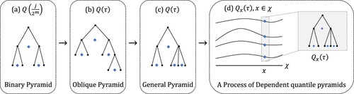
There is scope for a wide variety of choices for the distribution of the conditional medians of the subintervals (the $V_{m,j}$). If the $V_{m,j}$ are assumed to have mean 1/2, for example, then $Q^m\left(\tau \right)$ forms a martingale sequence and has a limit almost surely by Doob's martingale convergence theorem. Moreover, if $V_{m,j}$ are chosen so that $\underset{j\le 2^m}{max}\left\{Q^m\right(j/2^m)-Q^m((j-1)/2^m)\stackrel{p}{\to }0$, Hjort and Walker (2009) showed that there exists a continuous limiting quantile process to which $Q^m$ converges.

While Hjort and Walker (2009) primarily focussed on quantiles at the dyadic levels, we take inspiration from the oblique pyramid construction method introduced by Rodrigues et al. (2019a). In the oblique pyramid, quantile levels in a binary pyramid are not limited to dyadics.

2.2. General quantile pyramid

Rodrigues et al. (2019a) focus on finite quantile pyramids, where a pyramid has only M levels. They begin with scenarios where $2^{m-1}$ quantiles are generated at the $m^{th}$ level of a pyramid, ensuring that each subinterval contains one specified quantile. This constraint leads to exactly $2^M-1$ quantiles in an M-level pyramid. They then proceed to the oblique pyramid, a pyramid in which some subintervals contain a quantile but others do not. An M level pyramid may be unbalanced, specifying fewer than $2^M-1$ quantiles.

Rodrigues et al. (2019a) specify a rule for how the pyramid is constructed. We provide a brief example and refer the reader to their paper for full details. Consider the case of four quantiles, denoted as $Q\left({\tau }_1\right)<\dots <Q\left({\tau }_4\right)$. Since there are an even number of quantiles, there are two quantiles positioned in the middle. Following the rule of Rodrigues et al. (2019a), the smaller quantile serves as the middle quantile level. Thus, $Q\left({\tau }_2\right)$ is specified at the first level of the pyramid. Moving on to the second level, we have two subintervals. In the left subinterval, we specify $Q\left({\tau }_1\right)$, while the right subinterval contains two quantiles. The smaller quantile, $Q\left({\tau }_3\right)$, is specified at this level of the pyramid. In the third level, there are four subintervals: $(0,Q({\tau }_1\left)\right)$, $\left(Q\right({\tau }_1),Q({\tau }_2\left)\right)$, $\left(Q\right({\tau }_2),Q({\tau }_3\left)\right)$, $\left(Q\right({\tau }_3),1)$. In this level, we specify the remaining quantile, $Q\left({\tau }_4\right)$, in the last subinterval, while the other three subintervals remain empty. This example is illustrated in Figure 1(b).

We introduce additional flexibility by permitting non-binary splits. This yields the general quantile pyramid, and it empowers the user to fully customise the pyramid according to their preference. For instance, in the case of four quantiles, one can create a pyramid with $Q\left({\tau }_2\right)$ at the first level and the remaining three quantiles at the second level, distributing one quantile to the left subinterval and two to the right subinterval. This concept is visually represented in Figure 1(c). The move from a binary pyramid to a general pyramid requires novel notation which is introduced in the next section.

2.3. Dependent quantile pyramids

In the sequel, we extend the QP from a single distribution to a collection of distributions, creating a process of dependent quantile pyramids (DQPs). To do so, we construct a QP at each value of x in some index set, $\mathcal{X}$. We replace each scalar $V_{m,j}$ in Equation (1(1) $Q^m\left(j/2^m\right)=Q^{m-1}\left(\right(j-1\left)/2^m\right)(1-V_{m,j})+Q^{m-1}\left(\right(j+1\left)/2^m\right)V_{m,j},$(1) ) with an appropriate stochastic process, say $\{V_{x,m,j}$, $x\in \mathcal{X}\}$. This leads to a collection of QPs that may exhibit dependence across $\mathcal{X}$. Formally, we construct a distribution-valued stochastic process. For modelling purposes, the index set of the process is identified with the covariate space, as in QR. Alternatively, the index set may be described as containing values of predictors, spatial locations, constructed features, or time, to name a few possibilities. The important part is that, conditional on x, we have a model for a QP. We construct QPs on the unit interval $[0,1]$ following Hjort and Walker (2009) and use a general quantile pyramid scheme of Section 2.2. Figure 1(d) contains the visualisation of an example of a process of DQPs.

2.3.1. Notation

We write $Q_x\left(\tau \right)$ for the τ-quantile at x. For any x, $\left\{Q_x\right(\tau ),\tau \in (0,1\left)\right\}$ forms a complete quantile pyramid. For any τ, $\left\{Q_x\right(\tau ),x\in \mathcal{X}\}$ provides the τ-quantile surface over the covariate space. We refer to this as a QR curve. The DQP is constructed sequentially. To provide intuition behind the DQP and to facilitate proofs of its existence, we establish two distinct sets of notation.

The first set of notation matches the recursive construction of the DQP. We begin with a DQP with m−1 levels, where the quantile surfaces have been specified for $\tau \in {\mathcal{T}}_{m-1}$. That is, for $x\in \mathcal{X}$ and $\tau \in {\mathcal{T}}_{m-1}$, the function $\left\{Q_x\right(\tau ),x\in \mathcal{X},\tau \in$ ${\mathcal{T}}_{m-1}\}$ has already been determined in the sequential construction. The ordered quantile levels are ${\mathcal{T}}_{m-1}=\{{\tau }_1^{\ast },\dots ,{\tau }_T^{\ast }\}$, with ${\tau }_1^{\ast }<\dots <{\tau }_T^{\ast }$. At the next level, these quantile levels remain. The corresponding quantiles define a set of bands within which the quantiles newly specified at level m of the pyramid must lie (at a given x, the band is merely an interval). For example, the QR curve for a quantile $\tau \in ({\tau }_1^{\ast },{\tau }_2^{\ast })$ that is newly specifed at level m must lie in the band with lower boundary $\left\{Q_x\right({\tau }_1^{\ast }),x\in \mathcal{X}\}$ and upper boundary $\left\{Q_x\right({\tau }_2^{\ast }),x\in \mathcal{X}\}$. At level m, the specified quantiles are renumbered to form ${\mathcal{T}}_m$ and preserve the ordering of the ${\tau }_i^{\ast }$.

The second set of notation is preferred when describing the probability space that underlies the DQP. For this, we need to have each variable (with subscripts) refer to a single random element in the construction of the DQP. These variables appear in different positions in the pyramid. We introduce the ‘ϵ-notation’ to capture the position in the pyramid and to handle the potentially non-binary splits in the general quantile pyramid. Consider a pyramid with m levels. The sequential construction of the pyramid will place the quantile $Q_{x,{ϵ}_1}$ at level 1, $Q_{x,{ϵ}_1{ϵ}_2}$ at level 2, and so on. The length of the sequence indicates the level at which the quantile was specfied. The notation also conveys the structural relationship between quantiles. The parent quantiles of $Q_{x,{ϵ}_1\dots {ϵ}_m}$ are $Q_{x,{ϵ}_1\dots {ϵ}_{m-1}}$ and $Q_{x,{ϵ}_1\dots ({ϵ}_{m-1}+1)}$. If there are K quantiles specified in the interval between the parent quantiles, ${ϵ}_m$ takes a value in the set $1,\dots ,K$. The left and right parent quantiles have ${ϵ}_m=0$ and ${ϵ}_m=K+1$, respectively. The quantiles are increasing in ${ϵ}_m$. This results in two distinct sequences ${ϵ}_1\dots {ϵ}_m$ for a quantile that serves as both the left endpoint and the right endpoint of adjacent subintervals. As the construction proceeds, we use the left-endpoint sequence for which ${ϵ}_m=0$. For convenience, a short form $ϵ\equiv {ϵ}_1\cdots {ϵ}_{m-1}$ will be used for the $(m-1)$ length sequence throughout the paper. Figure 2 illustrates both notations for a three-level DQP with a given value of x.

Figure 2. An example of a DQP with covariate x with three levels and 13 quantiles. Both ${\tau }^{\ast }$ and ϵ-notation is shown. At level 0, the interval at each x is $[0,1]$. At level 1, K = 2 quantiles are specified, creating three subintervals. At level 2, four quantiles are newly specified, leading to a total of 7 subintervals. Notation for the newly specified quantiles is shown. At level 3, one quantile is specified within each subinterval. Both notations are shown for all quantiles in $(0,1)$. Collecting the quantiles across x gives the QR curves. The corresponding tree structure is the same across all values of x. It is shown in the right panel. Dots and rhombi represent subintervals and quantiles, respectively.

The oblique DQP is a special case in which all subintervals are split in two. In this case, K = 0 or 1 for all subintervals. For a dyadic, binary DQP, K = 1 for all subintervals and the quantile $Q_{x,{ϵ}_1\cdots {ϵ}_m}\left(\tau \right)$ at level m is the $\tau =\sum _{i=1}^m{ϵ}_i{2}^{-i}$ quantile of the distribution at x.

2.3.2. Definition

DQPs come in two main varieties. The first is the process of finite dependent quantile pyramids (FDQP) while the second, arrived at from a countable sequence of FDQPs, is termed the limit process of dependent quantile pyramids (LDQP).

We begin with the FDQP. The FDQP focuses on a finite number of quantiles. As with the QP, the FDQP is defined sequentially. We focus on the quantiles in a single interval (e.g. the centre interval at level 2 in Figure 2). The description applies to all such intervals.

Definition 2.1

We call $Q^M=\{Q_x^M,x\in \mathcal{X}\}$ a process of Finite Dependent Quantile Pyramids (FDQP) with M levels if there exists an M-level QP valued stochastic process whose distribution $Q^M$ follows. That is, for each $x\in \mathcal{X}$, $Q_x^M$ is an M-level QP on $[0,1]$, and, for each n and distinct $x_1,\dots ,x_n\in \mathcal{X}$, Kolmogorov's permutation and marginalization conditions are satisfied.

Definition 2.2

We call $F^M=\{F_x^M,x\in \mathcal{X}\}$ a set of conditional distribution functions induced by a process of FDQP with M levels, if for every $x\in \mathcal{X}$, $F_x^M$ is a distribution function and $F_x^M\left(Q_x^M\right(\tau \left)\right)=\tau$ for all $\tau \in (0,1)$.

The FDQP with M levels is given by its quantile functions, $\left\{Q_x^M\right(\tau ),x\in \mathcal{X},\tau \in [0,1\left]\right\}$. It is defined sequentially, beginning with level 1 of the pyramid. Assume that K quantiles are to be drawn at level m, for $m=1,\dots ,M$, in a subinterval that comes from level m−1. The subinterval is $(Q_{x,ϵ0},Q_{x,ϵ(K+1)})$ for $x\in \mathcal{X}$ and $ϵ={ϵ}_1\cdots {ϵ}_{m-1}$. The endpoints $Q_{x,ϵ0}$ and $Q_{x,ϵ(K+1)}$ are quantiles inherited from level m−1 of the pyramid. When m = 1, $Q_{x,ϵ0}=0$ and $Q_{x,ϵ(K+1)}=1$. Let $\{V_{x,{ϵ}_1\cdots {ϵ}_m},x\in \mathcal{X}\}$ be a multivariate stochastic process with index set $\mathcal{X}$. For each $x\in \mathcal{X}$ and $ϵ={ϵ}_1\cdots {ϵ}_{m-1}$ a random vector $(V_{x,ϵ1},\dots ,V_{x,ϵ(K+1)})$ follows a distribution with the following conditions: (1) $0<V_{x,ϵk}<1,\mathrm{f}\mathrm{o}\mathrm{r}k=1,\dots ,(K+1)$; and (2) $\sum _{k=1}^{K+1}{V}_{x,ϵk}=1$. That is, the vector lies in the interior of the K-dimensional simplex. The quantiles for the K specified quantile levels in the subinterval are (2) $Q_{x,ϵk}=Q_{x,ϵ0}(1-\sum _{j=1}^k{V}_{x,ϵj})+Q_{x,ϵ(K+1)}\left(\sum _{j=1}^k{V}_{x,ϵj}\right),k=1,\dots ,K.$(2) A finite number of quantiles, ${\tau }_1^{\ast }<\cdots <{\tau }_T^{\ast }$, is specified in the M-level pyramid. Quantiles that are not specified directly in the pyramid are given by linear interpolation. For all $\tau \in ({\tau }_t^{\ast },{\tau }_{t+1}^{\ast }),t=0,\dots ,T$, we linearly interpolate $Q_x^M\left(\tau \right)$, i.e. $Q_x^M\left(\tau \right)=Q_x^M\left({\tau }_t^{\ast }\right)+\left[Q_x^M\right({\tau }_{t+1}^{\ast })-Q_x^M({\tau }_t^{\ast }\left)\right](\tau -{\tau }_t^{\ast })/({\tau }_{t+1}^{\ast }-{\tau }_t^{\ast }).$The sequential construction and interpolation together define the conditional quantiles given x for all quantile levels $\tau \in (0,1)$.

In practice, when determining the number of quantiles, T, of an FDQP, we recognise that there is a tradeoff between the number of quantiles considered and computational efficiency. Our primary recommendation is to focus on the key quantiles of interest. A secondary, generic recommendation is to prioritise symmetric quantiles such as the three quartiles or the nine deciles.

The construction of the FDQP leads to its existence, which is formally proven in Lemma 3 in Section 3.2. At each value x, the distribution is defined by a finite collection of real valued random variates. The use of stochastic processes that are well-defined ensures that the QP construction for a single x extends to $\mathcal{X}$. We restrict attention to cases defined on a single probability space where the FDQP with M levels is the marginal distribution for each of the FDQPs with more than M levels, with appropriate renumbering of the quantiles in ${\cup }_{m=1}^M{\mathcal{T}}_m$, where ${\mathcal{T}}_m$ is the set of quantile levels specified at level m.

With some sufficient conditions, the limit may exist, in which case we have an infinite pyramid, leading to the LDQP. Our concern is with cases where a set of quantiles that is dense in $[0,1]$ is determined in the limit, and so we have no need for interpolation. The existence of the LDQP is established in Section 3.2. When the limit of a sequence of FDQPs exists as $m\to \mathrm{\infty }$, the limit process of dependent quantile pyramids (LDQP) is defined.

Definition 2.3

We call $Q=\{Q_x,x\in \mathcal{X}\}$ a limit process of Dependent Quantile Pyramids (LDQP) if there exists a QP valued stochastic process whose distribution Q follows. That is, for each $x\in \mathcal{X}$, $Q_x$ is a QP on $[0,1]$, and, for each n and distinct $x_1,\dots ,x_n\in \mathcal{X}$, Kolmogorov's permutation and marginalisation conditions are satisfied.

Definition 2.4

We call $F=\{F_x,x\in \mathcal{X}\}$ a set of conditional distribution functions induced by a process of LDQP, if for every $x\in \mathcal{X}$, $F_x$ is a distribution function and $Q_x\left(\tau \right)=inf\{y:F_x(y)\ge \tau \}$ for all $\tau \in (0,1)$.

2.4. Canonical construction

In this section, we provide a canonical construction of the quantiles in an arbitrary subinterval at level m of a process of DQPs. To do so, we construct U-processes and V-processes and then make use of Equation (2(2) $Q_{x,ϵk}=Q_{x,ϵ0}(1-\sum _{j=1}^k{V}_{x,ϵj})+Q_{x,ϵ(K+1)}\left(\sum _{j=1}^k{V}_{x,ϵj}\right),k=1,\dots ,K.$(2) ) in Section 2.3. We begin under the assumption that the choice of quantiles has been made and that this choice is consistent, matching the correct ordering of the quantiles. By repeatedly sampling U-processes and V-processes, we can proceed to sequential construction of the entire process of pyramids.

2.4.1. U-processes induced from Gaussian processes

Suppose that we are interested in obtaining K quantiles at level m for a subinterval $(Q_{x,ϵ0},Q_{x,ϵ(K+1)})$, $m\in \mathbb{N}$. For each sequence $ϵk$ for $k=1,\dots ,K+1$, we consider a Gaussian process (GP) $\{Z_{x,ϵk},x\in \mathcal{X}\}$ with zero mean, unit variance, and some correlation function $\lambda (x,x^{\prime })$, so that $Z_{x,ϵk}\sim \mathcal{G}\mathcal{P}(0,\lambda (x,x^{\prime }\left)\right).$ The correlation function governs the interdependence of quantiles across the covariate space. We note that the correlation function can differ for different $ϵk$.

We then construct the U-processes, $\{U_{x,ϵk},x\in \mathcal{X}\},k=1,\dots ,K+1$ for the subinterval, using the normal cumulative distribution function (cdf) transformation element-wise, i.e. for each $x\in \mathcal{X}$, $U_{x,ϵk}=\mathrm{\Phi }\left(Z_{x,ϵk}\right),$ where $\mathrm{\Phi }(\cdot )$ denotes the cdf of the standard normal distribution.

2.4.2. V-processes induced from U-processes via gamma variates

We construct the V-processes, $\{V_{x,ϵk},x\in \mathcal{X}\},k=1,\dots ,K+1$, from the U-processes. Let $G_{x,ϵk}(\cdot )$ be the gamma distribution function with shape ${\alpha }_{x,ϵk}>0$ and scale 1, for $k=1,\dots ,K+1$. For each $x\in \mathcal{X}$ and combination $ϵ={ϵ}_1\cdots {ϵ}_{m-1}$, define $Y_{x,ϵk}\equiv G_{x,ϵk}^{-1}\left(U_{x,ϵk}\right).$ Define $Y_x=\sum _{k=1}^{K+1}{Y}_{x,ϵk}$. Then, for each $x\in \mathcal{X}$ and ϵ, we set $(V_{x,ϵ1},\dots ,V_{x,ϵ(K+1)})\equiv (\frac{Y_{x,ϵ1}}{Y_x},\dots ,\frac{Y_{x,ϵ(K+1)}}{Y_x})$which forms a Dirichlet$({\alpha }_{x,ϵ1},\dots ,{\alpha }_{x,ϵ(K+1)})$ random vector. Lastly, collecting $V_{x,ϵk}$ together across $x\in \mathcal{X}$, we have constructed a vector-valued process $\left\{\right(V_{x,ϵ1},\dots ,V_{x,ϵ(K+1)}),x\in \mathcal{X}\}$ with component processes $\{V_{x,ϵk},x\in \mathcal{X}\}$, $k=1,\dots ,K+1.$ When ${\alpha }_{x,ϵk}$ and $G_{x,ϵk}$ do not depend on x, we omit the subscript x to simpify notation.

2.4.3. V-processes induced from U-processes via beta variates

The Dirichlet distribution can be derived from the product of independent beta random variates. This fact leads to a second construction of the V-processes. Define ${\alpha }_{x,ϵ1},\dots ,{\alpha }_{x,ϵ(K+1)}$ as before. Let $G_{x,ϵk}(\cdot )$ be the distribution function of a beta variate with parameters ${\alpha }_{x,ϵk}$ and $\sum _{j=k+1}^{K+1}{\alpha }_{x,ϵj}$. Define $Y_{x,ϵk}=G_{x,ϵk}^{-1}\left(U_{x,ϵk}\right)$ for each x and $k=1,\dots ,K$. Set $V_{x,ϵk}=Y_{x,ϵk}\prod _{j=1}^{k-1}(1-Y_{x,ϵj}),$with the conventions that an empty product is 1 and that $V_{x,ϵ(K+1)}=1-\sum _{k=1}^K{V}_{x,ϵk}$. The vector $(V_{x,ϵ1},\dots ,V_{x,ϵ(K+1)})$ follows a Dirichlet$({\alpha }_{x,ϵ1},\dots ,{\alpha }_{x,ϵ(K+1)})$ distribution.

Once V-processes are generated, we can proceed to the quantiles $Q_{x,ϵ1},\dots ,Q_{x,ϵK}$ in the subinterval, using Equation (2(2) $Q_{x,ϵk}=Q_{x,ϵ0}(1-\sum _{j=1}^k{V}_{x,ϵj})+Q_{x,ϵ(K+1)}\left(\sum _{j=1}^k{V}_{x,ϵj}\right),k=1,\dots ,K.$(2) ). Given the left and right endpoints of the subinterval, the conditional quantiles at the same quantile level can be expressed as a simple linear transformation of the V-processes. This observation also implies the preservation of the dependence structure. In other words, $\mathrm{C}\mathrm{o}\mathrm{r}\mathrm{r}(V_{x,ϵk},V_{x^{\prime },ϵk})=\mathrm{C}\mathrm{o}\mathrm{r}\mathrm{r}\left(\right[Q_{x,ϵk}|Q_{x,ϵ0},Q_{x,ϵ(K+1)}],[Q_{x^{\prime },ϵk}|Q_{x^{\prime },ϵ0},Q_{x^{\prime },ϵ(K+1)}\left]\right)$for any $x,x^{\prime }\in \mathcal{X}$ and ϵ, and for all $k=1,\dots ,K$. When K = 1 and the construction in this section is used, the random variable $V_{x,ϵ1}$ follows a beta distribution. It is a continuous, monotonic transformation of $U_{x,ϵ1}$. For measures of dependence that are invariant under such a transformation, the (conditional) dependence of $V_{x,ϵ1}$ and $V_{x^{\prime },ϵ1}$ matches that of $U_{x,ϵ1}$ and $U_{x^{\prime },ϵ1}$.

2.4.4. Martingale construction

One construction of the dyadic QP in Hjort and Walker (2009) relies on a martingale. At each level of the QP, each interval is split in half. In this canonical construction, K = 1 and the martingale property requires that ${\alpha }_{x,ϵ1}={\alpha }_{x,ϵ2}$ for a beta distribution. Allowing for splits that do not bisect the interval, this becomes, at level m of the pyramid, ${\alpha }_{x,ϵ1}=c_{x,m}({\tau }_{ϵ1}-{\tau }_{ϵ0})$ and ${\alpha }_{x,ϵ2}=c_{x,m}({\tau }_{ϵ2}-{\tau }_{ϵ1})$ for some $c_{x,m}>0$.

For a non-binary split of an interval, the values of ${\alpha }_{x,ϵk}$ need to be mapped to the relevant subintervals. Assume that a subinterval at the $m^{th}$ level contains quantiles associated with K specified quantile levels ${\tau }_{ϵ1}<\dots <{\tau }_{ϵK}$. Let ${\gamma }_{ϵk}$ for $k=1,\dots ,K$ denote the scaled quantile levels in the subinterval. The quantile levels of left and right endpoints of the subinterval are denoted by ${\tau }_{ϵ0}$ and ${\tau }_{ϵ(K+1)}$, respectively. Then ${\gamma }_{ϵk}=({\tau }_{ϵk}-{\tau }_{ϵ0})/({\tau }_{ϵ(K+1)}-{\tau }_{ϵ0}),k=1,\dots ,K.$From this, we can derive the values of ${\alpha }_{x,ϵk}$ satisfying the martingale condition. That is, ${\alpha }_{x,ϵk}=c_{x,m}({\tau }_{ϵk}-{\tau }_{ϵ(k-1)})$ for $k=1,\dots ,K+1$ and some $c_{x,m}>0$. We note that the chosen quantile levels ${\tau }_{ϵk}$ do not depend on x.

2.5. Quantile mapping for transitioning to the response space

Assume that the DQP has been constructed on $(0,1)$ and denote the QP at x by $Q_x\left(\tau \right)$. As briefly mentioned in Hjort and Walker (2009), we can transform the scale as for a proper response space, say, a real line using the inverse normal cdf transformation. Defining trend parameters ${\mu }_x$ and scale parameters ${\sigma }_x$, we have the canonical DQP regression model, centred on a normal theory regression: (3) $\left\{Q_x^{\mathbb{R}}\right(\tau )=\underset{\mathrm{T}\mathrm{r}\mathrm{e}\mathrm{n}\mathrm{d}}{\underbrace{{\mu }_x}}+\stackrel{\mathrm{L}\mathrm{o}\mathrm{c}\mathrm{a}\mathrm{l}\mathrm{F}\mathrm{l}\mathrm{u}\mathrm{c}\mathrm{t}\mathrm{u}\mathrm{a}\mathrm{t}\mathrm{i}\mathrm{o}\mathrm{n}}{\overbrace{\underset{\mathrm{S}\mathrm{c}\mathrm{a}\mathrm{l}\mathrm{e}}{\underbrace{{\sigma }_x}}\cdot {\mathrm{\Phi }}^{-1}\left(Q_x\right(\tau \left)\right)}},x\in \mathcal{X}\}.$(3) The trend parameter ${\mu }_x$ is shared across the quantiles and controls the overall trend of quantiles throughout the covariate space. The scale parameter controls the dispersion of the distributions while the realised QPs determine the departures from normality. Together, the scale and QP determine the departure (or local fluctuation) from a set of constant variance normal models with centres given by ${\mu }_x$.

Various choices can be made for the trend and scale. If one believes that there is no significant global trend, ${\mu }_x$ can be set to a constant. Alternatively, a linear regression model, ${\mu }_x=x^{\mathrm{\top }}\text{β}$, may provide an effective choice. The model is compatible with more complicated models for the trend. Similarly, models for ${\sigma }_x$ can range from a simple constant scale to more complex forms. The trend and scale parameters can be incorporated into Markov chain Monte Carlo (MCMC) procedures used to fit the model. Alternatively, to save computational effort, estimates can be plugged in and the parameters treated as fixed.

3. Theoretical results

The novel notation used in this section is formally defined in Appendix 1 while proofs of the results appear in Appendix 2.

3.1. A novel approach to existence of quantile pyramid

Hjort and Walker (2009) provide two different proofs for the existence of the QP. The following results establish the existence of the QP under slightly weaker conditions than those of Hjort and Walker (2009). They also apply to the oblique pyramid of Rodrigues et al. (2019a).

The QP is a probability measure for a distribution-valued random element. To show its existence, we wish to show that the sequence of probability measures that define the finite quantile pyramids (FQPs) converges to a limiting probability measure. Our argument relies on two key facts. First, the space of probability measures over distribution functions with support contained in $[0,1]$, when equipped with the Prokhorov metric, is compact (Parthasarathy 1967). Second, and yet to be established, the sequence of probability measures forms a Cauchy sequence. Together, these facts lead to the conclusion that the sequence of FQPs converges to a limit and that the limit is a probability measure on distribution-valued elements.

A first lemma bounds the Lévy distance, $d_L(\cdot ,\cdot )$, between two distribution functions that share a set of quantiles. Let $0={\tau }_0^{\ast }<{\tau }_1^{\ast }<{\tau }_2^{\ast }<\dots <{\tau }_T^{\ast }<{\tau }_{T+1}^{\ast }=1$ be ordered quantile levels. The largest gap between consecutive quantile levels appears in the bound below.

Lemma 3.1

Define $ϵ=\underset{t=1,\dots ,T+1}{max}({\tau }_t^{\ast }-{\tau }_{t-1}^{\ast })$. Assume that F and G are two distribution functions such that there exist $y_1,\dots ,y_T$ for which $F\left(y_t\right)=G\left(y_t\right)={\tau }_t^{\ast }$ for $t=1,\dots ,T$. Then, $d_L(F,G)\le ϵ$.

The construction of the QP proceeds through a sequence of FQPs, indexed by m, the number of levels in the pyramid. These FQPs are defined on a single probability space $(\mathrm{\Omega },\mathcal{B},\mu )$. Each $\omega \in \mathrm{\Omega }$ defines a sequence of FQPs with $m=1,2,\dots$ levels. The distributions in the sequence all have support contained in $[0,1]$ and share values of the quantile function at certain specified quantile levels, as described in Section 2.2. In particular, the ${\tau }_{{ϵ}_1\cdots {ϵ}_m}$ quantiles in $F^m\left(\omega \right)$ and $F^{m+k}\left(\omega \right)$ are identical for all ω and for any positive integer k. $\mathcal{B}$ is the Borel σ-field generated by the open sets under the Lévy metric.

The next lemma shows that the sequence of probability measures arising from the FQPs is Cauchy. The measure ${\mu }_m$ provides the probability distribution on $F^m$. The distance between ${\mu }_m$ and ${\mu }_n$ is measured by the Prokhorov metric, $d_P({\mu }_m,{\mu }_n)$.

Lemma 3.2

Suppose that ${\cup }_{m=1}^{\mathrm{\infty }}{\mathcal{T}}_m$ is dense in $[0,1]$. Then, under the Prokhorov metric $d_P$, the sequence $\{{\mu }_m{\}}_{m=1}^{\mathrm{\infty }}$ is a Cauchy sequence.

A Cauchy sequence on a compact set converges to a limit in the set. In this case, the sequence of measures ${\mu }_m$ converges to a limit measure μ. The limit measure is a probability measure on distribution-valued elements where the distributions have support contained in the interval $[0,1]$. This reasoning leads to the existence of the QP, stated formally in the next theorem. We note that the dyadic construction of the QP satisfies the denseness condition in Lemma 3.2.

Theorem 3.1

Suppose that ${\cup }_{m=1}^{\mathrm{\infty }}{\mathcal{T}}_m$ is dense in $[0,1]$. Then, the QP constructed as in Section 2.1 or 2.2 is a random element whose distribution is determined by $(\mathrm{\Omega },\mathcal{B},\mu )$.

3.2. Existence of a process of dependent quantile pyramids

The existence of a process of DQPs follows from consideration of the joint distributions of the QPs at finite sets of indices in the index set. The construction of the FDQP in Section 2.3 ensures the existence of the joint distribution of the corresponding sequence of FQPs. From here, the argument parallels that of the previous section, with the Lévy metric and Prokhorov metric replaced with their suprema over the finite set of indices. This ensures the existence of a probability space on which the limiting DQPs satisfy the requisite permutation and marginalisation conditions.

The DQP relies on a countable collection of real-valued stochastic processes, $V_{x,ϵk}$, all of which have index set $\mathcal{X}$. Each of these processes satisfies Komogorov's consistency axioms. The processes are defined on a single probability space. Selecting a finite set of distinct indices, say, $x_1,\dots ,x_n\in \mathcal{X}$, the sequence of FDQPs at these indices is generated by a countable collection of real-valued random variables. The permutation and marginalisation conditions follow immediately. This establishes the following lemma.

Lemma 3.3

Existence of FDQP

Under the conditions in the previous paragraph, for each $m\in \mathbb{N}$, there exists a distribution-valued stochastic process, $F^m=\{F_x^m,x\in \mathcal{X}\}$, with the specified finite dimensional distributions.

Define the suprema of the Lévy metric and Prokhorov metric over a set S to be $d_{L_u}(F^m,F^n)=\underset{x\in S}{sup}{d}_L(F_x^m,F_x^n)$ and $d_{P_u}({\mu }^m,{\mu }^n)=\underset{x\in S}{sup}{d}_P({\mu }_x^m,{\mu }_x^n)$, respectively. Lemma A.1 appearing in Appendix 2 shows that $d_{L_u}$ and $d_{P_u}$ are metrics. We first reprise Lemma 3.1.

Lemma 3.4

Define $ϵ=\underset{t=1,\dots ,T+1}{max}({\tau }_t^{\ast }-{\tau }_{t-1}^{\ast })$. Assume that $F_x$ and $G_x$, $x\in S$, are two sets of distribution functions such that, for each $x\in S$, there exist $y_{x,1},\dots ,y_{x,T}$ for which $F_x\left(y_{x,t}\right)=G_x\left(y_{x,t}\right)={\tau }_t^{\ast }$ for $t=1,\dots ,T$. Then, $d_{L_u}(F,G)\le ϵ$.

The construction of the FDQPs ensures that, for all ω, for each $x\in \{x_1,\dots ,x_n\}$ the ${\tau }_{{ϵ}_1\cdots {ϵ}_m}$ quantiles in $F_x^m\left(\omega \right)$ and $F_x^{m+k}\left(\omega \right)$ are identical for every positive integer k. This lets us apply the lemma. With a suitable choice of quantile levels, the sequence of probability measures for the set of n FQPs is Cauchy.

Lemma 3.5

Suppose that ${\cup }_{m=1}^{\mathrm{\infty }}{\mathcal{T}}_m$ is dense in $[0,1]$. Then, with $S=\{x_1,\dots ,x_n\}$, under the supremum Prokhorov metric $d_{P_u}$, the sequence $\{{\mu }_m{\}}_{m=1}^{\mathrm{\infty }}$ is a Cauchy sequence.

Finally, noting that the set of distributions with support contained in $[0,1{]}^n$ is compact under $d_{L_u}$, by Tychonoff's Theorem, we know that ${\mu }_m$ converges to some probability measure μ. This ensures the existence of the limiting DQP.

Theorem 3.2

Suppose that ${\cup }_{m=1}^{\mathrm{\infty }}{\mathcal{T}}_m$ is dense in $[0,1]$. Then, for any $S=\{x_1,\dots ,x_n\}\in \mathcal{X}$, the DQP for $x\in S$ constructed as in Section 2.3 is a random element whose distribution is determined by $(\mathrm{\Omega },\mathcal{B},\mu )$. Furthermore, there exists a stochastic process defined for all $x\in \mathcal{X}$ whose finite dimensional joint distributions on the QPs are exactly these.

4. Posterior inference

In this section, we discuss how to specify the DQP prior and the likelihood under the canonical construction. Suppose we have T quantiles of interest, ${\tau }_1^{\ast }<\cdots <{\tau }_T^{\ast }$, to be specified on the DQP. For simplicity, we work with the binary pyramid. A similar formulation can be laid out in the general case. Recall that with the canonical construction of the DQP in Section 2.4 and the canonical transformation in Section 2.5, quantiles are generated in the uniform scale and are transformed to the real line. For notational simplicity, we omit the superscript $\mathbb{R}$ from the quantile in (3(3) $\left\{Q_x^{\mathbb{R}}\right(\tau )=\underset{\mathrm{T}\mathrm{r}\mathrm{e}\mathrm{n}\mathrm{d}}{\underbrace{{\mu }_x}}+\stackrel{\mathrm{L}\mathrm{o}\mathrm{c}\mathrm{a}\mathrm{l}\mathrm{F}\mathrm{l}\mathrm{u}\mathrm{c}\mathrm{t}\mathrm{u}\mathrm{a}\mathrm{t}\mathrm{i}\mathrm{o}\mathrm{n}}{\overbrace{\underset{\mathrm{S}\mathrm{c}\mathrm{a}\mathrm{l}\mathrm{e}}{\underbrace{{\sigma }_x}}\cdot {\mathrm{\Phi }}^{-1}\left(Q_x\right(\tau \left)\right)}},x\in \mathcal{X}\}.$(3) ) and let $Q_x\left(\tau \right)$ denote the quantiles in the real line scale in this section.

4.1. Prior specification

A DQP $\left\{Q_x\right(\tau ),\tau \in (0,1\left)\right\}$ is defined for all $x\in \mathcal{X}$ as a stochastic process. Then, the finite-dimensional distributions of the DQP $\left(\right\{Q_{x_1}\left(\tau \right),\tau \in (0,1)\},\dots ,\{Q_{x_n}\left(\tau \right),\tau \in (0,1)\left\}\right)$ can be defined for each n-tuple $(x_1,\dots ,x_n)$ of distinct elements of $\mathcal{X}$ (Billingsley 1968). While the n-tuple can be arbitrary, in practice, we choose the coordinates to be covariate values for the data points.

Let the quantiles of interest be denoted by $Q$. For convenience, we view $Q$ as a $T\times n$ matrix. The $t^{th}$ row of $Q$ (denoted by $Q_{{\tau }_t^{\ast }}$) is the vector of the ${\tau }_t^{\ast }$ quantiles at $x_1,\dots ,x_n$ for $t=1,\dots ,T$. The ${\tau }_t^{\ast }$ quantile at $x_i$ is denoted by $Q_{x_i,{\tau }_t^{\ast }}$ for $i=1,\dots ,n$. The parent quantiles that defines the left and right endpoints of the interval on which $Q_{x_i,{\tau }_t^{\ast }}$ is generated are denoted by $Q_{x_i,{\tau }_t^{\ast }}^L$ and $Q_{x_i,{\tau }_t^{\ast }}^R$. The vectors $Q_{{\tau }_t^{\ast }}^L$ and $Q_{{\tau }_t^{\ast }}^R$ have $Q_{x_i,{\tau }_t^{\ast }}^L$ and $Q_{x_i,{\tau }_t^{\ast }}^R$ as their elements, respectively.

Write ${\mu }_x$ for the vector of trend transformation parameters and ${\sigma }_x$ for the vector of scale transformation parameters, where ${\mu }_{x_i}$ and ${\sigma }_{x_i}$ denote the element of ${\mu }_x$ and ${\sigma }_x$, respectively, corresponding to the value of $x_i$.

For a GP with zero mean given the input points $(x_1,\dots ,x_n)$, denoted by $Z$, let $\mathrm{\Lambda }=[{\lambda }_{x_i,x_j}{]}_{i,j=1}^n$ be the correlation matrix, where ${\lambda }_{x_i,x_j}=\lambda (x_i,x_j)$ is the correlation between $x_i$ and $x_j$ and ${\lambda }_{x_i,x_i}=1$. Let $\mathrm{\Psi }(\cdot ;a,b)$ denote the cdf of the $beta(a,b)$ distribution and $\mathrm{\Phi }(\cdot )$ and $\mathrm{\Phi }(\cdot ;\eta ,\nu )$ denote the cdfs of the $N(0,1)$ and the $N(\eta ,{\nu }^2)$ distribution, respectively.

Given the parameters $\mathrm{\Lambda },{\mu }_x,{\sigma }_x$, the joint conditional density of the finite dimensional distribution of the specified quantile levels of the DQP at $(x_1,\dots ,x_n)$ is $\pi (Q|\mathrm{\Lambda },{\mu }_x,{\sigma }_x)=\prod _{t=1}^T\{{\varphi }_n\left(h_1\right(Q_{x_1,{\tau }_t^{\ast }}),\dots ,h_n(Q_{x_n,{\tau }_t^{\ast }});0,\mathrm{\Lambda })\times \left|J\right({\tau }_t^{\ast }\left)\right|\},$where ${\varphi }_n(\cdot ;\eta ,V)$ denotes the probability distribution function (pdf) of the n-variate Normal, $N_n(\eta ,V)$, the back-transformed quantiles to the Z-scale $\begin{array}{rl}{h}_i\left(Q_{x_i,\tau }\right)& =h_i(Q_{x_i,\tau }|Q_{x_i,\tau }^L,Q_{x_i,\tau }^R,{\mu }_{x_i},{\sigma }_{x_i})\\ & ={\mathrm{\Phi }}^{-1}\left(\mathrm{\Psi }(\frac{\mathrm{\Phi }(Q_{x_i,\tau };{\mu }_{x_i},{\sigma }_{x_i})-\mathrm{\Phi }(Q_{x_i,\tau }^L;{\mu }_{x_i},{\sigma }_{x_i})}{\mathrm{\Phi }(Q_{x_i,\tau }^R;{\mu }_{x_i},{\sigma }_{x_i})-\mathrm{\Phi }(Q_{x_i,\tau }^L;{\mu }_{x_i},{\sigma }_{x_i})};a_{\tau },b_{\tau })\right),\end{array}$and the determinant of the Jacobian matrix is of the form $\begin{array}{rl}|J\left(\tau \right)|& =\prod _{i=1}^n\left|\frac{\mathrm{\partial }{h}_i(Q_{x_i,\tau }|Q_{x_i,\tau }^L,Q_{x_i,\tau }^R)}{\mathrm{\partial }{Q}_{x_i,\tau }}\right|\\ & =\prod _{i=1}^n\{\frac{1}{\varphi \left(Z_{x_i,\tau }\right)}\times \psi (\frac{\mathrm{\Phi }(Q_{x_i,\tau };{\mu }_{x_i},{\sigma }_{x_i})-\mathrm{\Phi }(Q_{x_i,\tau }^L;{\mu }_{x_i},{\sigma }_{x_i})}{\mathrm{\Phi }(Q_{x_i,\tau }^R;{\mu }_{x_i},{\sigma }_{x_i})-\mathrm{\Phi }(Q_{x_i,\tau }^L;{\mu }_{x_i},{\sigma }_{x_i})};a_{\tau },b_{\tau })\\ & \times \frac{\varphi (Q_{x_i,\tau };{\mu }_{x_i},{\sigma }_{x_i})}{\mathrm{\Phi }(Q_{x_i,\tau }^R;{\mu }_{x_i},{\sigma }_{x_i})-\mathrm{\Phi }(Q_{x_i,\tau }^L;{\mu }_{x_i},{\sigma }_{x_i})}\},\end{array}$where $\varphi (\cdot )$ and $\psi (\cdot ;a,b)$ denote the pdfs of the $N(0,1)$ and the $beta(a,b)$ distribution, respectively. The beta distribution parameters $a_{\tau }$ and $b_{\tau }$ can be established using the canonical choice outlined in Section 2.4. Given that we are working with the binary pyramid in this section where one quantile is estimated per subinterval, we can denote ${\tau }_t^{\ast }$ as ${\tau }_{ϵ1}$ using the ϵ-notation with an appropriate ϵ value. For $\tau ={\tau }_{x,ϵ1}$, we set $a_{\tau }={\alpha }_{x,ϵ1}$ and $b_{\tau }=1-{\alpha }_{x,ϵ1}$.

4.2. Updating

Since we use the normal distribution for the transformation from $[0,1]$ to $\mathbb{R}$, the conditional density of the response variable is piecewise-normal. Given the values of the covariate $X=[x_1\cdots x_n{]}^{\mathrm{\top }}$ and the parameters $Q,{\mu }_x$, and ${\sigma }_x$, the pdf of $Y$ is $f(y|Q,{\mu }_x,{\sigma }_x)=\prod _{i=1}^n\left[\sum _{t=1}^{T+1}\frac{({\tau }_t^{\ast }-{\tau }_{t-1}^{\ast })\times I_{\left(Q_{x_i}\right({\tau }_{t-1}^{\ast }),Q_{x_i}({\tau }_t^{\ast }\left)\right]}\left(y_i\right)\times \varphi (y_i;{\mu }_{x_i},{\sigma }_{x_i})}{\mathrm{\Phi }\left(Q_{x_i}\right({\tau }_t^{\ast });{\mu }_{x_i},{\sigma }_{x_i})-\mathrm{\Phi }\left(Q_{x_i}\right({\tau }_{t-1}^{\ast });{\mu }_{x_i},{\sigma }_{x_i})}\right],$where $I_A\left(x\right)$ is an indicator function whose value is one when $x\in A$ and zero otherwise.

Utilizing the information present in the data through the likelihood, we can update the prior in Section 4.1 via a MCMC procedure with a Metropolis-Hastings step. More details can be found in Appendix 3. If desired, variations on the basic algorithm can be used to improve the mixing of the Markov chain.

4.3. Inference for the DQP

Posterior inference can be made based on the DQP prior and likelihood using the MCMC procedure in Appendix 3. An estimate of a set of QR curves under squared error loss is obtained by taking the posterior mean of the sample of quantiles at each x.

The dependence across the covariate space is fundamental to the DQP framework. The conditional quantiles are intrinsically dependent on one another through both the GP correlation structure, $\mathrm{\Lambda }$, and the pyramid structure. Typically, increasing the level of dependence results in smoother QR curves, while reducing dependence leads to more flexible and bumpier QR curves.

4.3.1. Linearized inference under the DQP

Bayesian methods allow one to distinguish between beliefs about a quantity, say a QR curve, and inference about the quantity. One strategy that has proven successful is to perform modelling in a large space and to impose parsimony through a restriction on the inference (e.g. MacEachern 2001; Hahn and Carvalho 2015). In contrast, practitioners of classical statistics generally impose parsimony by working in a smaller model space or through model selection.

Much of the literature on QR, both classical and Bayesian, focuses on linear QR. The DQP model naturally produces a posterior distribution that assigns probability one to nonlinear QR curves. To linearise inference, one needs a distribution over the covariate and a set of draws from the posterior distribution of the QR curve.

As a criterion, we minimise the integrated squared difference between the nonlinear QR curves and a linear QR curve. That is, with x following a distribution G and a quantile level of interest τ, and presuming the following integrals are finite, (4) $\begin{array}{rl}\text{*}{\text{β}}_L\left(\tau \right)& =\arg \underset{\text{*}{\text{β}}^{\ast }}{min}(\int \int (Q_{x,\tau }-x^{\mathrm{\top }}\text{*}{\text{β}}^{\ast }{)}^2\mathrm{d}P\left(Q_{x,\tau }\right)\mathrm{d}G\left(x\right))\\ & =\arg \underset{\text{*}{\text{β}}^{\ast }}{min}(\int ({\mathbb{E}}_x\left[Q_{x,\tau }\right]-x^{\mathrm{\top }}\text{*}{\text{β}}^{\ast }{)}^2\mathrm{d}G\left(x\right)),\end{array}$(4) where $P(\cdot )$ denotes a posterior distribution function of $Q_{x,\tau }$ and ${\mathbb{E}}_x[\cdot ]$ denotes the expectation of the quantity at each x.

In practice, if lacking a distribution G, we use the empirical cdf of x for G and the posterior mean of the conditional quantiles to estimate ${\mathbb{E}}_x\left[Q_{x,\tau }\right]$. With this particular choice, this minimisation is obtained as a least squares fit on the posterior mean of the conditional quantiles. The same ${\text{β}}_L\left(\tau \right)$ can be obtained in a second fashion. First, map the nonlinear QR curve at each MCMC iterate to the best fitting linear QR curve with a least squares fit. Then map this collection of linear QR curves values to the overall best linear QR curve via a second least squares regression of the least squares fits on x. More details are contained in Appendix 3.

4.3.2. Quantile prediction for a new x value

We can obtain a posterior predictive distribution of quantiles for a new x value, denoted as $x^{\ast }$. This is achieved by following a two-step algorithm. First, we run an MCMC algorithm to sample mapping parameters and DQPs from their joint posterior distribution at the covariate locations where data points exist, namely $x_1,\dots ,x_n$. Next, for a given MCMC iterate, we sample the DQP at the new value $x^{\ast }$ from its conditional posterior distribution.

We empasize one important point. In the event that there is no existing data point at $x^{\ast }$, the conditional posterior distribution is just the conditional prior distribution. By collecting the sampled quantiles at the new value $x^{\ast }$, we are able to construct the marginal posterior predictive distribution of quantiles for that specific location. For details on how to perform the posterior sampling of quantiles and mapping parameters from their respective posterior distributions, please refer to Section 4.2.

5. Simulation study

We conducted simulation studies to evaluate how the DQP performs. We considered two sets of quantiles: $T=3(0.25,0.50,0.75)$ and $T=7(0.05,0.10,0.25,0.50,0.75,0.90,0.95)$. The covariate is $x_{ij}=i$ and the response is $Y_{ij}$ for $i=1,\dots ,10$ and $j=1,\dots ,r$. Let $N(0,1)$ denote the standard normal distribution and $t_{df}$ a t-distribution with df degrees of freedom. We considered the following three scenarios for the simulation study.

Scenario 1. (Homogeneous Error) $Y_{ij}=x_{ij}+{ϵ}_{ij},\mathrm{w}\mathrm{h}\mathrm{e}\mathrm{r}\mathrm{e}{ϵ}_{ij}\stackrel{iid}{\sim }F$ Scenario 2. (Heterogeneous Error) $Y_{ij}=x_{ij}+{ϵ}_{ij},\mathrm{w}\mathrm{h}\mathrm{e}\mathrm{r}\mathrm{e}{ϵ}_{ij}\stackrel{iid}{\sim }\{\begin{array}{ll}\sqrt{10}F& \mathrm{i}\mathrm{f}5\le i\le 6\\ F& \mathrm{o}\mathrm{t}\mathrm{h}\mathrm{e}\mathrm{r}\mathrm{w}\mathrm{i}\mathrm{s}\mathrm{e}\end{array}$ Scenario 3. (Nonlinear association between the covariate and the response)

1. $Y_{ij}=\sin \left(x_{ij}\right)+{ϵ}_{ij},\mathrm{w}\mathrm{h}\mathrm{e}\mathrm{r}\mathrm{e}{ϵ}_{ij}\stackrel{iid}{\sim }N(0,1)$

2. $Y_{ij}=\exp \left(1/x_{ij}\right)+{ϵ}_{ij},\mathrm{w}\mathrm{h}\mathrm{e}\mathrm{r}\mathrm{e}{ϵ}_{ij}\stackrel{iid}{\sim }N(0,1)$

For Scenarios 1 and 2, (1) $F=N(0,1)$; (2) $F=t_{20}$; (3) $F=t_3$. Scenario 1 examines the case where the error variance is homogeneous and the normality assumption used in the mapping from $(0,1)$ to $\mathbb{R}$ is satisfied (1-1), slightly violated (1-2), and more severely violated (1-3). In Scenario 2, the error variance is not constant, with a larger variance for certain covariate values, and the mapping is correctly specified (2-1), slightly misspecified (2-2), or more severely misspecified (2-3). Finally, Scenario 3 showcases settings where the error is normally distributed with homogeneous variance, but the covariate and response variables have a nonlinear association.

For each setting, we used r = 10 and r = 30 replicates at each value of x, corresponding to overall sample sizes of n = 100 and n = 300, respectively. In each of our 32 scenario-T-sample size combinations, we generated S = 100 data sets, fit QRs, and calculated the empirical mean-squared error (MSE) for each quantile τ at $x\in \mathcal{X}$: ${\mathrm{M}\mathrm{S}\mathrm{E}}_x\left(\tau \right)=\frac{1}{S}\sum _{s=1}^S\left({\hat{Q}}_x^s\right(\tau )-Q_x(\tau ){)}^2,$ where ${\hat{Q}}_x^s\left(\tau \right)$ is an estimated quantile for τ level with $s^{th}$ simulated data set at x. We further computed the MSE for the quantile, averaged over the distribution of x as $\mathrm{M}\mathrm{S}\mathrm{E}\left(\tau \right)=\sum _{x=1}^{10}0.1{\mathrm{M}\mathrm{S}\mathrm{E}}_x\left(\tau \right)$, which again is averaged over τ as $\mathrm{A}\mathrm{M}\mathrm{S}\mathrm{E}=\sum _{t=1}^T\sum _{x=1}^{10}0.1{\mathrm{M}\mathrm{S}\mathrm{E}}_x\left(\tau \right)/T$.

We fit a binary FDQP with two levels for the T = 3 case and with three levels for the T = 7 case based on the normal inverse cdf transformation from (3(3) $\left\{Q_x^{\mathbb{R}}\right(\tau )=\underset{\mathrm{T}\mathrm{r}\mathrm{e}\mathrm{n}\mathrm{d}}{\underbrace{{\mu }_x}}+\stackrel{\mathrm{L}\mathrm{o}\mathrm{c}\mathrm{a}\mathrm{l}\mathrm{F}\mathrm{l}\mathrm{u}\mathrm{c}\mathrm{t}\mathrm{u}\mathrm{a}\mathrm{t}\mathrm{i}\mathrm{o}\mathrm{n}}{\overbrace{\underset{\mathrm{S}\mathrm{c}\mathrm{a}\mathrm{l}\mathrm{e}}{\underbrace{{\sigma }_x}}\cdot {\mathrm{\Phi }}^{-1}\left(Q_x\right(\tau \left)\right)}},x\in \mathcal{X}\}.$(3) ), centreing the FDQP on a linear regression model with ${\mu }_x=x^{\mathrm{\top }}\text{β}$. Regarding the dependence of the pyramids between locations x and $x^{\prime }$ in the covariate space, we used the canonical construction for the Gaussian processes with zero mean vector and Gaussian correlation function $\lambda (x,x^{\prime })=\exp (-\Vert x-x^{\prime }{\Vert }^2/\varphi )$ with $\varphi =5$. For the beta distribution at level m in the construction of the binary pyramid prior, we used ${\alpha }_{ϵ1}=c_m({\tau }_{ϵ1}-{\tau }_{ϵ0})$ and ${\alpha }_{ϵ2}=c_m({\tau }_{ϵ2}-{\tau }_{ϵ1})$ with $c_m=(m+5{)}^2$. The prior distribution for $\text{β}$ is bivariate normal with mean ${\mu }_0=(5,0{)}^{\mathrm{\top }}$ and variance matrix ${\mathrm{\Sigma }}_0=\text{diag}(3,3)$. For the scale transformation parameter ${\sigma }_x$, we used the sample standard deviation at x as a plug-in estimator.

We compare our method to four alternatives: a classical QR approach by Koenker and Bassett (1978) (‘quantreg’), a Bayesian QR approach by Yu and Moyeed (2001) implemented by Benoit and Van den Poel (2017) (‘bayesQR’), a simultaneous linear QR by Yang and Tokdar (2017) (‘qrjoint’), and its generalised variant incorporating spatial dependence using a Gaussian process by Chen and Tokdar (2021) (‘JSQR-GP’). The estimators are evaluated by AMSE. For the MCMC runs of bayesQR, qrjoint, JSQR-GP, and DQP, we used a warmup of 1, 000 iterates followed by 100, 000 draws for estimation, thinned at a rate of 1 in 100.

The AMSE values are summarised in Figure 3, while the corresponding values and standard errors can be found in Tables A1 and A2 in Appendix 4. Examining Figure 3, the linearised DQP (‘DQP-lm’) demonstrated competitive performance relative to the alternative approaches in Scenario 1. It either had the lowest AMSE or had an AMSE within a two standard error range of the lowest value for all of the cases of Scenarios 1-1 and 1-2 except for the T = 7 and n = 100 case. This suggests that when the underlying relationship between the response and covariates is believed to be linear, the DQP can be effectively used for linear inference, yielding reasonable results. In Scenario 1, qrjoint had the lowest AMSE in most cases, primarily because its linearity assumption in the model closely aligns with the underlying truth and it simultaneously estimates multiple conditional quantiles. We note that DQP struggled when the normal assumption in scale transformation of DQP is severely violated (Scenario 1-3).

Figure 3. AMSE values for each combination of scenario-T-sample size.

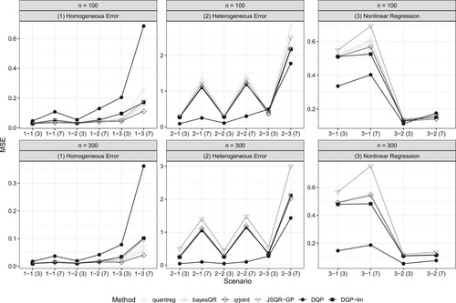
Under Scenarios 2-1 and 2-2, the DQP ourperformed all other methods. This is because the DQP is not only robust to mild misspecification of the mapping from $(0,1)$ to the response variable scale but can also account for the local nonlinearity arising from a larger variance at specific locations of the covariate. Among the linear methods, DQP-lm performed the best. This observation may be attributed to the fact that DQP-lm identifies linear QR curves by leveraging the QR curves estimated within the nonlinear model space. Even under Scenario 2-3, where the normal assumption in the DQP transformation is violated, the DQP still outperformed other methods in most of the cases except when n = 100 and T = 7.

Regarding the nonlinear association between the covariate and the response, represented by Scenarios 3-1 and 3-2, the DQP has lower AMSE than the other alternatives for most combinations of n and the number of quantiles, except for the case of n = 100 and T = 7 under Scenario 3-2. This is because the DQP can capture the local nonlinearity of quantiles, such as the cyclic movement in Scenario 3-1 and the sudden drop for small covariate values in Scenario 3-2. The advantage of the DQP becomes more evident as n increases.

6. Application

Elsner et al. (2008) observed that the trend in tropical cyclone intensity in the North Atlantic Ocean from 1981 to 2006 is different for different quantiles. They fit separate linear QRs for multiple quantiles using the R package ‘quantreg’ (Koenker 2005) and found that the higher quantiles showed an upward trend, with statistically significant slopes above the 0.7 quantile. Lower quantiles had slopes closer to zero.

Kadane and Tokdar (2012) analysed the same data set and came to a different conclusion. They developed a Bayesian approach to simultaneously fit a collection of linear QRs. They found that the increasing trend in the cyclone intensity was significant for almost all quantiles, not just the upper quantiles.

We analysed the data set (https://myweb.fsu.edu/jelsner/temp/Data.html) from Elsner et al. (2008). The data consist of the lifetime maximum wind speeds of 291 North Atlantic tropical cyclones derived from satellite imagery. The wind speeds are the response (Y) and range from 29.8 to $159.5{\mathrm{m}\mathrm{s}}^{-1}$. The year is the covariate (x).

We fit a binary FDQP with four levels and 15 quantiles at τ = 0.05, 0.10, 0.20, 0.25, 0.30, 0.35, 0.40, 0.50, 0.60, 0.65, 0.70, 0.75, 0.80, 0.90, and 0.95. We used the binary canonical construction with Gaussian processes with zero mean vector and the exponential correlation function $\lambda (x,x^{\prime })=\exp (-\Vert x-x^{\prime }\Vert /\varphi )$ with $\varphi =5$. For the beta distribution at level m in the construction of V processes, we used ${\alpha }_{ϵ1}=c_m({\tau }_{ϵ1}-{\tau }_{ϵ0})$ and ${\alpha }_{ϵ2}=c_m({\tau }_{ϵ2}-{\tau }_{ϵ1})$ with $c_m=(m+5{)}^2$. We again used the canonical transformation with linear regression model for the trend parameter, i.e. ${\mu }_x=x^{\mathrm{\top }}\text{β}$. The prior distribution for $\text{β}$ is bivariate normal with mean ${\mu }_0=(75,0.5{)}^{\mathrm{\top }}$ and variance matrix ${\mathrm{\Sigma }}_0=\text{diag}(15,2)$. For the scale transformation parameter ${\sigma }_x$, we fitted an ordinary least squares model with the sample standard deviation regressed on each year and then used the resulting fitted values. We ran 10, 000 warm up iterates of MCMC followed by 200, 000 iterates, thinned to 2, 000 iterates for estimation. For the purpose of comparison, we also applied the alternative simultaneous QR methods discussed in Section 5 to the same dataset.

Figure 4 displays the analysis results from the simultaneous QR methods, including our approach. In panel (a), the grey lines provide the posterior means at each year and the black lines the linearised fit. The lines are overlaid on the data points. The 95% credible intervals for the slopes of the linearised fit are shown in the right panel of (a). The slopes tend to be greater for greater quantiles, implying that stronger cyclones have been getting stronger more quickly. Indeed, the 95% credible interval for the slope of the 0.95 quantile is observed to be well above that of the 0.50 quantile. This means that the most intense cyclones are increasing in strength at a significantly faster rate than the moderately strong cyclones. The 95% credible intervals for the slope of the quantiles below 0.50 include zero. The slopes do not significantly differ from zero for lower quantiles. Overall, our method applied to these data shows the intensity of the upper half of the cyclones to be increasing, with more powerful cyclones intensifying at a more rapid rate.

Figure 4. Left column: 15 estimated quantiles of cyclone intensity with grey data points. Right column: Estimated slopes of the quantile lines with 95% empirical credible intervals. In (a), grey lines are the posterior means of the quantiles and black lines are the linearised fit of the posterior mean.

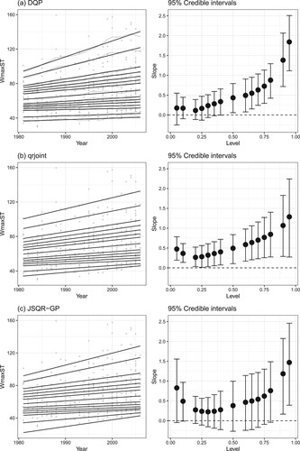
On the other hand, the outcome obtained from qrjoint in panel (b) reveals that all the 95% credible intervals lie above zero while overlapping with one another. This suggests that cyclone intensities are increasing across all levels, although the rate of increase may not significantly differ among cyclones with varying power. Meanwhile, the findings from JSQR-GP in panel (c) indicate that only the slopes for the strongest cyclones have values greater than zero, with their respective intervals also overlapping. While we lack knowledge of the absolute ground truth, it becomes evident that all three models concur on one point: the intensity of the strongest cyclones is increasing.

7. Discussion

We propose a nonparametric Bayesian approach to quantile regression, based on a process of DQPs. The DQP generalises the QP of Hjort and Walker (2009) to allow dependence across a predictor space. The flexibility of the model allows us to depart from linearity and to handle regressions for multiple quantiles in unbounded predictor spaces without quantile crossing.

The canonical construction can be adapted to account for a various features of the data. As examples, the standard normal distribution used in the inverse cdf transformation can be replaced with a distribution with different tails to handle thick or thin tailed data; skewness in the quantiles can be handled by replacing the symmetric normal distribution with an asymmetric distribution; and positively valued responses can be handled by basing the transformation on a distribution supported on the half line. The linear regression model for the mean can be replaced with a nonlinear form, resulting in large-scale nonlinearity of the QRs. Simple choices for this include the use of a deterministic form such as a fixed-knot spline or a stochastic form such as a Gaussian process. Replacement of the linear form for the scale factor (say, $x^{\mathrm{\top }}\gamma$) with a form that ensures positivity, for example, $\exp \left(x^{\mathrm{\top }}\gamma \right)$, relieves concerns about the implications of unbounded $\mathcal{X}$.

In the simulation examples, we employed the sample standard deviation at the location x as a plug-in estimator for the scale transformation parameter ${\sigma }_x$. An alternative is to use a pooled sample standard deviation in situations where heterogeneity is not suspected, such as Scenario 1. The results of this alternative will be included in our future work. The simulations we report above rely on a single predictor. The stochastic processes used for the FDQP are Gaussian processes that are then passed through transformations to arrive at the FDQP. Extension to the case of multiple predictors is straightforward through the use of Gaussian processes with a multivariate index. The Gaussian processes can be replaced with other processes.

Acknowledgments

The authors wish to thank the reviewers for comments that improved the paper.

Disclosure statement

No potential conflict of interest was reported by the author(s).

Additional information

Funding

The authors gratefully acknowledge support from National Science Foundation grants DMS-2015552 and SES-1921523.

Appendices

Appendix 1

• $(\mathrm{\Omega },\mathcal{B},\mu )$ := a triple that defines a probability space

• D = the space of all distributions with the support on $[0,1]$

• $D_S$ = the product space of all collections of (conditional) distributions with the support on $[0,1]$ on some finite set $S\subset \mathcal{X}$

• ${\mathcal{B}}^{\prime }$ := the Borel σ-field of D, i.e. all Borel sets of distributions on D

• ${\mathcal{B}}_S^{\prime }$ := the Borel σ-field of $D_S$

• $d_L(F,G)$ := Lévy metric between distributions F and G ($F,G\in D$)

• $d_L(F,A)=inf\left\{d_L\right(F,G)|G\in A\}$ := Lévy metric between a distribution $F\in D$ and a Borel set $A\in {\mathcal{B}}^{\prime }$

• $A_{\alpha }=\{F\in D|d_L(F,A)<\alpha \}$ := the open α ball ($\alpha >0$) about $A\in {\mathcal{B}}^{\prime }$ (or $A_{\alpha }=\{F\in D|d_{L_u}(F,A)<\alpha \}$ for $A\in {\mathcal{B}}_S^{\prime }$)

• $\mathcal{P}=\mathcal{P}\left({\mathcal{B}}^{\prime }\right)$ := all Borel probability measures on the Borel σ-field of D

• ${\mathcal{P}}_S={\mathcal{P}}_S\left({\mathcal{B}}_S^{\prime }\right)$ := all Borel probability measures on the Borel σ-field of $D_S$

• $d_P(\mu ,\nu )$ := the Prokhorov metric on $\mathcal{P}$ for $\mu ,\nu \in \mathcal{P}$, that is $d_P(\mu ,\nu )=\underset{\alpha >0}{inf}\left\{\alpha |\mu \right(A)\le \nu (A_{\alpha })+\alpha \text{ and }\nu (A)\le \mu (A_{\alpha })+\alpha \text{ for all }A\in {\mathcal{B}}^{\prime }\}$

• $F^m$ := an m-level FQP in Section 3.1 and FDQP in Section 3.2

• ${\mathrm{\Omega }}_{A,m}=\left\{\omega |F^m\right(\omega )\in A\}$ := an ω-set with $F^m$ and $A\in {\mathcal{B}}^{\prime }$

• ${\mathrm{\Omega }}_{A_{\alpha },m}=\left\{\omega |F^m\right(\omega )\in A_{\alpha }\}$ := the α ball for $F^m\left(\omega \right)$ about $A\in {\mathcal{B}}^{\prime }$

• ${\mu }_m$ := a probability measure in $\mathcal{P}$ arising from all the m-level pyramids, which assigns probabilities to subsets of D (or $D_S$ for some $S\subset \mathcal{X}$)

• ${\mu }_m\left(A\right)=\mu \left({\mathrm{\Omega }}_{A,m}\right)$ := the probability that the probability distributions induced from m-level pyramids belong to $A\in {\mathcal{B}}^{\prime }$

Appendix 2

Proof

Proof of Lemma 3.1

Consider $y\in [{\tau }_{t-1}^{\ast },{\tau }_t^{\ast }]$. Then ${\tau }_{t-1}^{\ast }\le F\left(y\right),G\left(y\right)\le {\tau }_t^{\ast }$. Thus $F\left(y\right)-ϵ\le {\tau }_t^{\ast }-ϵ\le {\tau }_{t-1}^{\ast }$ and so $F\left(y\right)-ϵ\le G\left(y\right)$. Similarly, $F\left(y\right)+ϵ\ge {\tau }_{t-1}^{\ast }+ϵ\ge {\tau }_t^{\ast }$ and so $F\left(y\right)+ϵ\ge G\left(y\right)$. Thus $F(y-ϵ)-ϵ\le G\left(y\right)\le F(y+ϵ)+ϵ$. Repeating the argument above for $t=1,\dots ,T+1$ establishes that $d_L(F,G)\le ϵ$.

Proof

Proof of Lemma 3.2

Fix $ϵ>0$. Choose M such that $\underset{t\in \{1,\dots ,T_M+1\}}{max}({\tau }_t^{\ast }-{\tau }_{t-1}^{\ast })<ϵ$. Applying Lemma 3.1, we have $d_L\left(F^m\right(\omega ),F^n(\omega \left)\right)<ϵ$ for all $m,n\ge M$ and for all $\omega \in \mathrm{\Omega }$. That is, $F^n\left(\omega \right)$ is in the ϵ-ball about $F^m\left(\omega \right)$. Such an M always exists provided that ${\cup }_{m=1}^{\mathrm{\infty }}{\mathcal{T}}_m$ is dense in $[0,1]$ and each $F^m\left(\omega \right)$ has the same pyramid structure.

Consider an arbitrary Borel set $A\in {\mathcal{B}}^{\prime }$. Define the sets ${\mathrm{\Omega }}_{A,m}=\left\{\omega |F^m\right(\omega )\in A\}$ and ${\mathrm{\Omega }}_{A_{ϵ},n}=\left\{\omega |F^n\right(\omega )\in A_{ϵ}\}$. For every $\omega \in {\mathrm{\Omega }}_{A,m}$, $F^n\left(\omega \right)$ is in the ϵ-ball about $F^m\left(\omega \right)$. Hence $\omega \in {\mathrm{\Omega }}_{A_{ϵ},n}$ and so ${\mathrm{\Omega }}_{A,m}\subset {\mathrm{\Omega }}_{A_{ϵ},n}$.

Turning to the probability measures on the FQPs with m and n levels, we note that ${\mu }_m\left(A\right)=\mu \left({\mathrm{\Omega }}_{A,m}\right)$ and ${\mu }_n\left(A_{ϵ}\right)=\mu \left({\mathrm{\Omega }}_{A_{ϵ},n}\right)$. Since ${\mathrm{\Omega }}_{A,m}\subset {\mathrm{\Omega }}_{A_{ϵ},n}$, ${\mu }_m\left(A\right)\le {\mu }_n\left(A_{ϵ}\right)<{\mu }_n\left(A_{ϵ}\right)+ϵ$. A similar argument shows that ${\mu }_n\left(A\right)<{\mu }_m\left(A_{ϵ}\right)+ϵ$. This holds for all Borel A, and so $d_P({\mu }_m,{\mu }_n)\le ϵ$. Thus, for each $ϵ>0$, there is an M such that, for all $m,n\ge M$, $d_P({\mu }_m,{\mu }_n)\le ϵ$. The sequence $\{{\mu }_m{\}}_{m=1}^{\mathrm{\infty }}$ is Cauchy.

Proof

Proof of Theorem 3.1

By Lemma 3.2, the sequence $\{{\mu }_m{\}}_{m=1}^{\mathrm{\infty }}$ is Cauchy. Moreover, the space $\mathcal{P}$ equipped with the Prokhorov metric is compact, and thus complete, since the space D equipped with Lévy metric is compact (see Theorem 2.6.4 in Parthasarathy 1967). Therefore, the sequence $\{{\mu }_m{\}}_{m=1}^{\mathrm{\infty }}$ is convergent. That is, there exists μ to which ${\mu }_m$ converges and that μ provides a probability distribution on $\underset{m\to \mathrm{\infty }}{lim}{F}^m$. Thus, a limit of QP exists.

Lemma A.1

$d_{L_u}$ as defined in Section 3.2 is a metric on the space of distributions. $d_{P_u}$ is a metric on the space of probability measures over distributions. The set $\mathcal{S}$ need not have finite cardinality.

Proof.

Symmetry, non-negativity, the triangle inequality, and the zero property follow from straightforward calculation. With a nod to the St. Petersburg paradox, we must show that $d_{L_u}(F^m,F^n)<\mathrm{\infty }$. Since $d_L(F_x^m,F_x^n)\le 1$ for all $x\in \mathcal{S}$, we have that $d_{L_u}(F^m,F^n)\le 1$. The argument for $d_{P_u}$ is established in the same way.

Proof

Proof of Lemma 3.4

From Lemma 3.1, we have $d_L(F_x,G_x)\le ϵ$ for all $x\in \mathcal{S}$. Thus $d_{L_u}(F,G)\le ϵ$.

Proof

Proof of Lemma 3.5

Replace $d_L$ with $d_{L_u}$, $d_P$ with $d_{P_u}$, and ${\mathcal{B}}^{\prime }$ with ${\mathcal{B}}_S^{\prime }$ in the proof of Lemma 3.2.

Proof

Proof of Theorem 3.2

The proof of the first part of the theorem follows that of Theorem 3.1. Kolmogorov's permutation condition is satisfied at each step in the sequence of FDQPs since each of the $V_x$ processes satisfies the condition. His marginalisation condition is also satisfied. Since $\{x_1,\dots ,x_n\}$ was arbitrary, this ensures the existence of a stochastic process with the specified limiting distributions (e.g. Billingsley 1968, chapter 7).

Appendix 3

A.1. MCMC algorithms

1. Sample $Q=[Q_{{\tau }_1},\dots ,Q_{{\tau }_T}{]}^{\mathrm{\top }}$ given ${\mu }_x$ and ${\sigma }_x$

   1. Choose ${\tau }_t$ following the top-down pyramid structure.

   2. Sample $Q_{{\tau }_t}^p=(Q_{x_1,{\tau }_t}^p,\dots ,Q_{x_n,{\tau }_t}^p{)}^{\mathrm{\top }}$ given the neighbouring quantiles $Q_{{\tau }_{t-1}}=(Q_{x_1,{\tau }_{t-1}},\dots ,Q_{x_n,{\tau }_{t-1}}{)}^{\mathrm{\top }}$ and $Q_{{\tau }_{t+1}}=(Q_{x_1,{\tau }_{t+1}},\dots ,Q_{x_n,{\tau }_{t+1}}{)}^{\mathrm{\top }}$, for $t=1,\dots ,T$ from a conditional proposal density $q(\cdot |Q_{-{\tau }_t},{\mu }_x,{\sigma }_x)$.

   3. Accept the new proposal $Q^p$ whose $t^{th}$ row is replaced with $Q_{{\tau }_t}^p$ over the current value $Q^c$ with probability $\alpha =min\{1,\frac{\pi (Q^p|{\mu }_x,{\sigma }_x)f(y|Q^p,{\mu }_x,{\sigma }_x)}{\pi (Q^c|{\mu }_x,{\sigma }_x)f(y|Q^c,{\mu }_x,{\sigma }_x)}\times \frac{q(Q_{{\tau }_t}^c|Q_{-{\tau }_t},{\mu }_x,{\sigma }_x)}{q(Q_{{\tau }_t}^p|Q_{-{\tau }_t},{\mu }_x,{\sigma }_x)}\}.$

   4. Repeat (i)–(iii) until the bottom of the pyramid.

2. Sample ${\mu }_x$ given $Q$ and ${\sigma }_x$

   1. Partition ${\mu }_x$ into I blocks. Call block i ${\mu }_x^i$.

   2. Sample ${\mu }_x^{\left(i\right),p}$ from a conditional proposal density $q(\cdot |{\mu }_x^{\left(i\right),c})$ and accept with probability $\alpha =min\{1,\frac{\pi \left({\mu }_x^{\left(i\right),p}|{\mu }_x^{-\left(i\right)}\right)f(y|Q,{\mu }_x^p,{\sigma }_x)}{\pi \left({\mu }_x^{\left(i\right),c}|{\mu }_x^{-\left(i\right)}\right)f(y|Q,{\mu }_x^c,{\sigma }_x)}\times \frac{q\left(\pi \right({\mu }_x^{\left(i\right),c}|{\mu }_x^{\left(i\right),p})}{q\left(\pi \right({\mu }_x^{\left(i\right),p}|{\mu }_x^{\left(i\right),c})}\}.$

   3. Repeat step (ii) for $i=1,\dots ,I$.

3. Sample ${\sigma }_x$ given $Q$ and ${\mu }_x$ following a similar step to 2.

Note that the sampling of $Q$ can be further broken down to sampling of smaller blocks as in step 2. Doing so impacts the acceptance rate of the proposals and the mixing of the Markov chain.

A.2. Linearized inference

Throughout this derivation, we assume that the integrals are finite. This ensures the non-trivial existence of a minimizing ${\text{β}}^{\ast }$. $\begin{array}{rl}{\text{β}}_L\left(\tau \right)& =\arg \underset{{\text{β}}^{\ast }}{min}(\int \int (Q_{x,\tau }-x^{\mathrm{\top }}{\text{β}}^{\ast }{)}^2\mathrm{d}P\left(Q_{x,\tau }\right)\mathrm{d}G\left(x\right))\\ & =\arg \underset{{\text{β}}^{\ast }}{min}(\int \int (Q_{x,\tau }-{\mathbb{E}}_x\left[Q_{x,\tau }\right]+{\mathbb{E}}_x\left[Q_{x,\tau }\right]-x^{\mathrm{\top }}{\text{β}}^{\ast }{)}^2\mathrm{d}P\left(Q_{x,\tau }\right)\mathrm{d}G\left(x\right))\\ & =\arg \underset{{\text{β}}^{\ast }}{min}(\int \int (Q_{x,\tau }-{\mathbb{E}}_x\left[Q_{x,\tau }\right]{)}^2\mathrm{d}P\left(Q_{x,\tau }\right)\mathrm{d}G\left(x\right)\\ & +\int \int ({\mathbb{E}}_x[Q_{x,\tau }]-x^{\mathrm{\top }}{\text{β}}^{\ast }{)}^2\mathrm{d}P(Q_{x,\tau }\left)\mathrm{d}G\right(x)\\ & +\int \int 2(Q_{x,\tau }-{\mathbb{E}}_x[Q_{x,\tau }\left]\right)({\mathbb{E}}_x[Q_{x,\tau }]-x^{\mathrm{\top }}{\text{β}}^{\ast })\mathrm{d}P\left(Q_{x,\tau }\right)\mathrm{d}G\left(x\right))\\ & =\arg \underset{{\text{β}}^{\ast }}{min}(\int ({\mathbb{E}}_x\left[Q_{x,\tau }\right]-x^{\mathrm{\top }}{\text{β}}^{\ast }{)}^2\mathrm{d}G\left(x\right)),\end{array}$where $P(\cdot )$ denotes the posterior distribution function of $Q_{x,\tau }$, $G(\cdot )$ denotes the distribution function of x, and ${\mathbb{E}}_x[\cdot ]$ denotes the expectation of the quantity at each x. Moreover, if $G\left(x\right)$ is the empirical cdf of x, then the problem above becomes ${\text{β}}_L\left(\tau \right)=\arg \underset{{\text{β}}^{\ast }}{min}\left(\sum _{i=1}^n\frac{1}{n}\right({\mathbb{E}}_x\left[Q_{x,\tau }\right]-x_i^{\mathrm{\top }}{\text{β}}^{\ast }{)}^2),$which is equivalent to the least squares linear regression problem.

Appendix 4

Table E1. AMSE values over 100 simulated datasets with standard errors in parentheses when n = 100.

Scenario	T	quantreg	bayesQR	qrjoint	JSQR-GP	DQP	DQP-lm
1-1	3	0.0353	0.0293	0.0277	0.0314	0.0463	0.0301
		(0.0035)	(0.0029)	(0.0028)	(0.0038)	(0.0032)	(0.0031)
	7	0.0574	0.0421	0.0350	0.0405	0.1076	0.0510
		(0.0055)	(0.0042)	(0.0034)	(0.0042)	(0.0058)	(0.0051)
1-2	3	0.0395	0.0323	0.0304	0.0328	0.0540	0.0331
		(0.0035)	(0.0030)	(0.0028)	(0.0029)	(0.0035)	(0.0033)
	7	0.0702	0.0506	0.0404	0.0461	0.1293	0.0530
		(0.0076)	(0.0054)	(0.0039)	(0.0044)	(0.0064)	(0.0050)
1-3	3	0.0541	0.0449	0.0448	0.0534	0.2043	0.0959
		(0.0066)	(0.0055)	(0.0049)	(0.0059)	(0.0176)	(0.0108)
	7	0.2531	0.1551	0.1113	0.1788	0.6842	0.1712
		(0.0321)	(0.0180)	(0.0135)	(0.0241)	(0.0642)	(0.0195)
2-1	3	0.2937	0.2809	0.2788	0.2809	0.0861	0.2636
		(0.0059)	(0.0049)	(0.0050)	(0.0085)	(0.0058)	(0.0038)
	7	1.3685	1.1694	1.1271	1.2326	0.2460	1.1033
		(0.0511)	(0.0187)	(0.0117)	(0.0321)	(0.0166)	(0.0080)
2-2	3	0.3021	0.2917	0.2888	0.2844	0.1041	0.2762
		(0.0061)	(0.0056)	(0.0054)	(0.0049)	(0.0069)	(0.0041)
	7	1.4621	1.2579	1.2129	1.3279	0.2958	1.1887
		(0.0525)	(0.0170)	(0.0110)	(0.0287)	(0.0185)	(0.0073)
2-3	3	0.3832	0.3679	0.3641	0.3828	0.4922	0.4434
		(0.0087)	(0.0073)	(0.0068)	(0.0112)	(0.0944)	(0.0206)
	7	2.8263	2.2268	2.1619	2.4989	1.7753	2.1811
		(0.1651)	(0.0434)	(0.0390)	(0.0885)	(0.3882)	(0.0539)
3-1	3	0.5219	0.5192	0.5099	0.5486	0.3356	0.5105
		(0.0053)	(0.0048)	(0.0041)	(0.0074)	(0.0063)	(0.0041)
	7	0.5869	0.6074	0.5684	0.6910	0.4031	0.5253
		(0.0116)	(0.0104)	(0.0080)	(0.0150)	(0.0094)	(0.0055)
3-2	3	0.1365	0.1302	0.1292	0.1384	0.1134	0.1324
		(0.0035)	(0.0033)	(0.0030)	(0.0042)	(0.0037)	(0.0030)
	7	0.1661	0.1633	0.1408	0.1615	0.1756	0.1526
		(0.0071)	(0.0063)	(0.0043)	(0.0061)	(0.0068)	(0.0049)

Table E2. AMSE values over 100 simulated datasets with standard errors in parentheses when n = 300.

Scenario	T	quantreg	bayesQR	qrjoint	JSQR-GP	DQP	DQP-lm
1-1	3	0.0116	0.0105	0.0100	0.0113	0.0175	0.0092
		(0.0012)	(0.0011)	(0.0010)	(0.0012)	(0.0010)	(0.0009)
	7	0.0183	0.0148	0.0133	0.0144	0.0367	0.0151
		(0.0019)	(0.0016)	(0.0013)	(0.0015)	(0.0018)	(0.0014)
1-2	3	0.0134	0.0121	0.0105	0.0120	0.0195	0.0106
		(0.0014)	(0.0013)	(0.0010)	(0.0011)	(0.0012)	(0.0010)
	7	0.0239	0.0199	0.0153	0.0171	0.0417	0.0176
		(0.0024)	(0.0021)	(0.0015)	(0.0017)	(0.0022)	(0.0016)
1-3	3	0.0179	0.0163	0.0147	0.0269	0.0781	0.0343
		(0.0017)	(0.0017)	(0.0014)	(0.0092)	(0.0075)	(0.0036)
	7	0.0765	0.0587	0.0401	0.0964	0.3621	0.1015
		(0.0086)	(0.0065)	(0.0041)	(0.0282)	(0.0504)	(0.0133)
2-1	3	0.2593	0.2571	0.2561	0.4969	0.0434	0.2409
		(0.0026)	(0.0026)	(0.0024)	(0.0922)	(0.0035)	(0.0015)
	7	1.1491	1.1068	1.0972	1.3953	0.0965	1.0521
		(0.0162)	(0.0103)	(0.0107)	(0.0750)	(0.0072)	(0.0026)
2-2	3	0.2714	0.2681	0.2654	0.4406	0.0454	0.2503
		(0.0030)	(0.0031)	(0.0025)	(0.0901)	(0.0039)	(0.0014)
	7	1.2422	1.1992	1.1776	1.4726	0.0986	1.1391
		(0.0193)	(0.0122)	(0.0071)	(0.0728)	(0.0064)	(0.0025)
2-3	3	0.3386	0.3359	0.3287	0.5408	0.2687	0.3596
		(0.0040)	(0.0040)	(0.0032)	(0.1143)	(0.0557)	(0.0097)
	7	2.1926	2.0864	2.0261	3.0027	1.4277	2.1116
		(0.0338)	(0.0208)	(0.0155)	(0.5633)	(0.4497)	(0.0539)
3-1	3	0.4944	0.4937	0.4907	0.5675	0.1457	0.4790
		(0.0023)	(0.0024)	(0.0020)	(0.0109)	(0.0034)	(0.0013)
	7	0.5555	0.5547	0.5427	0.7533	0.1866	0.4825
		(0.0065)	(0.0059)	(0.0048)	(0.0184)	(0.0051)	(0.0016)
3-2	3	0.1115	0.1102	0.1091	0.1191	0.0530	0.1083
		(0.0014)	(0.0014)	(0.0011)	(0.0024)	(0.0017)	(0.0010)
	7	0.1232	0.1214	0.1158	0.1368	0.0755	0.1144
		(0.0025)	(0.0023)	(0.0017)	(0.0038)	(0.0028)	(0.0016)

References

- Benoit, D.F., and Van den Poel, D. (2017), ‘bayesQR: A Bayesian Approach to Quantile Regression’, Journal of Statistical Software, 76, 1–32.
- Billingsley, P. (1968), Convergence of Probability Measures, New York: John Wiley & Sons.
- Bissiri, P.G., Holmes, C.C., and Walker, S.G. (2016), ‘A General Framework for Updating Belief Distributions’, Journal of the Royal Statistical Society: Series B (Statistical Methodology), 78(5), 1103–1130.
- Chen, X., and Tokdar, S.T. (2021), ‘Joint Quantile Regression for Spatial Data’, Journal of the Royal Statistical Society: Series B (Statistical Methodology), 83(4), 826–852.
- Chen, C., and Yu, K. (2009), ‘Automatic Bayesian Quantile Regression Curve Fitting’, Statistics and Computing, 19, 271–281.
- Edgeworth, F.Y. (1888), ‘The Mathematical Theory of Banking’, Journal of the Royal Statistical Society, 51(1), 113–127.
- Elsner, J.B., Kossin, J.P., and Jagger, T.H. (2008), ‘The Increasing Intensity of the Strongest Tropical Cyclones’, Nature, 455, 92–95.
- Geraci, M., and Bottai, M. (2007), ‘Quantile Regression for Longitudinal Data Using the Asymmetric Laplace Distribution’, Biostatistics, 8(1), 140–154.
- Hahn, P.R., and Carvalho, C.M. (2015), ‘Decoupling Shrinkage and Selection in Bayesian Linear Models: a Posterior Summary Perspective’, Journal of the American Statistical Association, 110(509), 435–448.
- Hjort, N.L., and Walker, S.G. (2009), ‘Quantile Pyramids for Bayesian Nonparametrics’, The Annals of Statistics, 78(1), 105–131.
- Kadane, J.B., and Tokdar, S.T. (2012), ‘Simultaneous Linear Quantile Regression: a Semiparametric Bayesian Approach’, Bayesian Analysis, 7(1), 51–72.
- Koenker, R. (2005), Quantile Regression, Econometric Society Monographs, Cambridge: Cambridge University Press.
- Koenker, R. (2017), ‘Quantile Regression: 40 Years on’, Annual Review of Economics, 9, 155–176.
- Koenker, R., and Bassett, G. (1978), ‘Regression Quantiles’, Econometrica: Journal of the Econometric Society, 46(1), 33–50.
- Kottas, A., and Krnjajić, M. (2009), ‘Bayesian Semiparametric Modelling in Quantile Regression’, Scandinavian Journal of Statistics, 36(2), 297–319.
- Kotz, S., Kozubowski, T., and Podgórski, K (2001), The Laplace Distribution and Generalizations: a Revisit with Applications to Communications, Economics, Engineering, and Finance, Boston: Springer Science & Business Media.
- Kozumi, H., and Kobayashi, G. (2011), ‘Gibbs Sampling Methods for Bayesian Quantile Regression’, Journal of Statistical Computation and Simulation, 81(11), 1565–1578.
- Lum, K., and Gelfand, A.E. (2012), ‘Spatial Quantile Multiple Regression Using the Asymmetric Laplace Process’, Bayesian Analysis, 7(2), 235–258.
- MacEachern, S.N. (2001), ‘Decision Theoretic Aspects of Dependent Nonparametric Processes’, in Bayesian Methods with Applications to Science, Policy and Official Statistics, pp. 551–560. Crete: International Society for Bayesian Analysis.
- Parthasarathy, K.R (1967), Probability Measures on Metric Spaces, New York: Academic Press Inc.
- Parzen, E. (2004), ‘Quantile Probability and Statistical Data Modeling’, Statistical Science, 19, 652–662.
- Reich, B.J. (2012), ‘Spatiotemporal Quantile Regression for Detecting Distributional Changes in Environmental Processes’, Journal of the Royal Statistical Society: Series C (Applied Statistics), 61(4), 535–553.
- Reich, B.J., Bondell, H.D., and Wang, H.J. (2010), ‘Flexible Bayesian Quantile Regression for Independent and Clustered Data’, Biostatistics, 11(2), 337–352.
- Reich, B.J., Fuentes, M., and Dunson, D.B. (2011), ‘Bayesian Spatial Quantile Regression’, Journal of the American Statistical Association, 106(493), 6–20.
- Rodrigues, T., Dortet-Bernadet, J.-L., and Fan, Y. (2019a), ‘Pyramid Quantile Regression’, Journal of Computational and Graphical Statistics, 28(3), 732–746.
- Rodrigues, T., Dortet-Bernadet, J.-L., and Fan, Y. (2019b), ‘Simultaneous Fitting of Bayesian Penalised Quantile Splines’, Computational Statistics & Data Analysis, 134, 93–109.
- Rodrigues, T., and Fan, Y. (2017), ‘Regression Adjustment for Noncrossing Bayesian Quantile Regression’, Journal of Computational and Graphical Statistics, 26(2), 275–284.
- Taddy, M.A., and Kottas, A. (2010), ‘A Bayesian Nonparametric Approach to Inference for Quantile Regression’, Journal of Business & Economic Statistics, 28(3), 357–369.
- Tsionas, E.G. (2003), ‘Bayesian Quantile Inference’, Journal of Statistical Computation and Simulation, 73(9), 659–674.
- Waldmann, E., Kneib, T., Yue, Y.R., Lang, S., and Flexeder, C. (2013), ‘Bayesian Semiparametric Additive Quantile Regression’, Statistical Modelling, 13(3), 223–252.
- Yang, Y., and Tokdar, S.T. (2017), ‘Joint Estimation of Quantile Planes Over Arbitrary Predictor Spaces’, Journal of the American Statistical Association, 112(519), 1107–1120.
- Yu, K., and Moyeed, R.A. (2001), ‘Bayesian Quantile Regression’, Statistics & Probability Letters, 54(4), 437–447.
Appendices
Appendix 1
:= a triple that defines a probability space