Good-bootstrap: simultaneous confidence intervals for large alphabet distributions

Abstract

Simultaneous confidence intervals (SCI) for multinomial proportions are a corner stone in count data analysis and a key component in many applications. A variety of schemes were introduced over the years, mostly focussing on an asymptotic regime where the sample is large and the alphabet size is relatively small. In this work we introduce a new SCI framework which considers the large alphabet setup. Our proposed framework utilises bootstrap sampling with the Good-Turing probability estimator as a plug-in distribution. We demonstrate the favourable performance of our proposed method in synthetic and real-world experiments. Importantly, we provide an exact analytical expression for the bootstrapped statistic, which replaces the computationally costly sampling procedure. Our proposed framework is publicly available at the first author's Github page.

Keywords:

• Simultaneous confidence intervals
• multinomial distribution
• good-turing
• large alphabet
• count data

1. Introduction

Consider a multinomial distribution p over an alphabet size m. Let $X^n\triangleq \{X_1,\dots ,X_n\}$ be a collection of nn independent and identically distributed samples from pp. In this work we study simultaneous confidence intervals (SCIs) for pp. This problem was extensively studied over the years, with several notable contributions such as Quesenberry and Hurst (1964), Goodman (1964), Fitzpatrick and Scott (1987) and Sison and Glaz (1995). Current methodologies focus on two basic setups. The first considers an asymptotic regime, where the sample size is very large (Quesenberry and Hurst 1964; Goodman 1964; Sison and Glaz 1995). The second addresses the case where both the sample and the alphabet are relatively small (Chafai and Concordet 2009; Malloy et al. 2020). In this work we study the complementary case, where the alphabet size is large, or at least comparable, to the sample size. This setup is also known as the large alphabet regime.

Large alphabet modelling is of special interest in many applications such as language processing and bioinformatics (Orlitsky and Suresh 2015). One of the typical challenges in this setup is the inference of rare events. Specifically, the probability of symbols that do not appear in the sample (unseen symbols). Here, classical tools tend to underestimate the desired parameters (Orlitsky et al. 2003) and more sophisticated schemes are required. The problem of estimating p in the large alphabet regime was extensively studied in the context of point estimation. Probably the first to address this problem was Laplace (1825). In his work, Laplace suggested adding a single count to every symbol in the alphabet. This way, unseen symbols are inferred as if they have a single count in the sample. A major milestone to large alphabet point estimation was achieved in the work of I.J. Good and A.M. Turing during world war II, while deciphering the German Enigma Code (Good 1953). Good and Turing proposed a surprisingly efficient and unintuitive framework which assigns symbols with k appearance a probability proportional to the number of events that appear k + 1 times. Since its appearance the Good-Turing estimator has gained popularity in a variety of fields. To this day, Good-Turing estimators are perhaps the most commonly used methods in practical setups (Orlitsky and Suresh 2015).

In this paper, we study interval estimation for the multinomial proportions in large alphabet regimes. We propose a new approach which applies bootstrap sampling with the Good-Turing estimator as the plug-in distribution. We demonstrate the performance of our suggested scheme in a series of synthetic and real-world experiments. We show it outperforms popular alternatives, as it attains significantly smaller SCIs while maintaining the prescribed coverage rate.

2. Related work

We distinguish between two setups of interest. The first, considers the case where nn is large (asymptotic), compared to the alphabet size, while the second addresses the case where both n and m are small. In the first regime, Quesenberry and Hurst (1964) suggested joint confidence intervals based on large sample properties of the sample proportions and the inversion of Pearson's chi-square goodness-of-fit test. The intervals control the joint coverage probability for all possible linear combinations of the parameters. Therefore, these intervals are necessarily conservative, often wider than necessary, with larger coverage than required (May and Johnson 1997). Goodman (1964) proposed an adaptation for Quesenbeny and Hurst by using the Bonferroni inequality, making them less conservative and thus shorter for the same confidence level. Fitzpatrick and Scott (1987) introduced an adaptation of the binomial distribution to the multinomial scheme by finding a lower bound for the simultaneous coverage probability of all binomial symbols CIs together. Perhaps the most popular scheme for large n is of Sison and Glaz (1995). In their work, Sison and Glaz (SG) used the connection between the Poisson, truncated Poisson and multinomial distributions to derive an alternative formulation for the joint multinomial probability, which is then approximated by Edgeworth expansions. They showed Through extensive simulations that their method leads to smaller SCIs while maintaining a coverage rate closer to the desired level, compared to known methods at the time. Unfortunately, the SG algorithm does not perform well in terms of coverage in cases where m is large, or the expected symbol counts are disparate (May and Johnson 1997). In their review survey, May and Johnson (1997) performed simulation studies to compare different SCIs methods. They recommended the Goodman intervals for cases where the sample size supports the large sample theory, m is small and the expected counts are at least ten per symbol. For cases where the expected symbol counts are small and nearly equal across all symbols, they recommended using SG intervals. No method was uniformly superior for every examined setup. Moreover, typically one cannot assess the expected symbol counts prior to the experiment. All the methods above are popular and well-established SCIs schemes. Unfortunately, they all assume an asymptotic regime in their derivation. Consequently, they perform quite poorly in cases of small sample size, small number of observed symbol frequencies or sampling zeros (May and Johnson 1997).

The second line of work addresses the case where both n and m are small. Here, Chafai and Concordet (2009) and later (Malloy et al. 2020) introduced optimal (exact) CRs for multinomial proportions which generalise classical results for Binomial distributions (the well-known Clopper-Pearson CI). Unfortunately, their framework is computationally exhaustive and does not scale to large alphabets.In fact, it requires heavy enumeration of order of $n^m$, which makes it impractical for relatively small n and m.

It is important to emphasise that SCIs may also be obtained from a binomial viewpoint, where each symbol is treated in turn against all other symbols. That is, one may construct a binomial CI for each symbol independently and correct for multiplicity. Henceforth, the SCIs are just a collection of binomial CIs of confidence level $\alpha /m$ for every symbol in the alphabet. Naturally, this approach controls the prescribed confidence level (for every n and m), but may be over pessimistic and result in large volume SCIs. Notice that such an approach also applies for unobserved symbols. Specifically, the binomial CI for symbols with zero counts is obtained by the rule-of-three, which suggests $[0,-\log (\alpha /m)/n]$ (Vysochanskij and Petunin 1980).

The problem of large alphabet probability estimation is of great interest and was extensively studied over the years, mostly in the context of point estimation. One of the major challenges when dealing with large alphabets is under sampled symbols. This problem is mostly evident in cases where some symbols are not sampled at all (for example, consider n<m). Historically, Laplace (1825) was perhaps the first to address this problem (Zabell 1989). In his estimation scheme, a single count is added to every symbol in the alphabet, followed by maximum likelihood estimation. This solution guarantees that no symbols are missing from the sample. Laplace's scheme was later generalised to a family of add-constant estimators, where instead of adding a single count, a constant number c is added. The add-constant estimators are very simple and practical. Unfortunately, they preform quite poorly is cases where the alphabet size is much larger than the sample (Orlitsky et al. 2003).

During World War II, in an effort to decipher the Enigma Code, Good and Turing (Good 1953) developed an alternative method for estimating the proportions of large multinomial distributions. The basic Good-Turing framework considers an estimator for symbols that appear t times in the sample. Formally, (1) ${\hat{p}}_t=\frac{{\phi }_{t+1}}{{\phi }_t}\cdot \frac{t+1}{n},$(1) where ${\phi }_t$ is the number of symbols appearing t times in the sample. In words, the probability of the symbols that appear t times in the sample is proportional to the number of symbols that appear t + 1 times. Hence, non-sampled probabilities are assigned a probability proportional to the number of events with a single appearance in the sample. Notice that as opposed to the add-constant estimators, the Good-Turing estimator is oblivious to the alphabet size, which makes it more robust. The Good-Turing estimator has gained great popularity and was applied to a variety of fields. Perhaps its most common application is in language modelling, where it is used to estimate the probability distribution of words (Orlitsky and Suresh 2015). On the theoretical side, interpretations of the Good-Turing estimator have been proposed (Nadas 1985; Good 2000) and its favourable properties were studied (McAllester and Schapire 2000; Orlitsky and Suresh 2015; Painsky 2021, 2022b, 2022a).

In practice, it was shown that the original GT scheme (1(1) ${\hat{p}}_t=\frac{{\phi }_{t+1}}{{\phi }_t}\cdot \frac{t+1}{n},$(1) ) is sub-optimal for symbols that appear more frequently (Gale and Sampson 1995). This problem is addressed by several adaptations. Gale and Sampson (1995) proposed a smoothed version of the algorithm which utilises linear regression to smooth the erratic values. Another approach is to use an hybrid scheme, which applies GT for low frequency symbols and maximum likelihood for symbols that appear many times (Painsky 2022b). An additional example, which we utilise later in this work, was introduced by Orlitsky and Suresh (2015). Specifically, (2) ${\hat{p}}_t=\{\begin{array}{ll}\frac{t}{n}& \mathrm{if}t>{\phi }_{t+1}\\ \frac{{\phi }_{t+1}+1}{{\phi }_t}\cdot \frac{t+1}{n^{\ast }}& \mathrm{else},\end{array}$(2) where $n^{\ast }$ is a normalisation factor. Notice that the term ${\phi }_{t+1}$ in the original Good-Turing formulation (1(1) ${\hat{p}}_t=\frac{{\phi }_{t+1}}{{\phi }_t}\cdot \frac{t+1}{n},$(1) ) is replaced with ${\phi }_{t+1}+1$ to ensure that every symbol is assigned a non-zero probability.

3. Problem statement

Let $\mathcal{X}$ be a finite alphabet of size m. Let $p=p_1,\dots ,p_m$ be an unknown probability distribution over $\mathcal{X}$. Let $X\sim p$ be a random variable taking values over $\mathcal{X}$. Let $X^n=\{X_1,\dots ,X_n\}$ be a collection of n independent and identically distributed samples from $\mathcal{X}$. In this work we study rectangular confidence region (RCR) for the probability distribution vector p. A RCR of level $100(1-\alpha )\mathrm{\%}$ for p is defined as a region $S(X^n)$ such that $P(p\in S(X^n))\ge 1-\alpha$where $S(X^n)=S_1(X^n),S_2(X^n),\dots ,S_m(X^n)$, and $S_i(X^n)=[a_i,b_i]$ for $i=1,\dots ,m$. We naturally have that, $0\le a_i\le b_i\le 1$. In other words, a RCR for p in defined by a collection SCIs, for every symbol distribution such that, $P(p\in S(X^n))=P(\bigcap _{i=1}^m\{p_i\in S_i(X^n)\})\ge 1-\alpha$SCIs are very popular in multinomial inference, as they are intuitive and easy to interpret. In fact, almost all the RCRs discussed in Section 2 are in fact SCIs. Naturally, there are many ways to construct SCIs that satisfy the above (for example, $a_i=0,b_i=1$ for all i). We are interested in minimal volume SCIs that satisfy the prescribed coverage probability. As mentioned above, we focus on the large alphabet regime, where m is relatively large, compared to n.

4. Methodology

Our proposed method utilises bootstrap sampling to construct SCIs. Specifically, we focus on the plug-in principle, with several adaptations that account for the large alphabet regime. We begin this section with a brief overview of the bootstrap paradigm for inference problems.

4.1. Bootstrap confidence intervals

Bootstrap sampling is a popular approach for inference problems, especially in cases where the underlying distribution is involved or too complicated to analyse. By using the bootstrap principle we typically avoid the assumptions needed in classical analytical inference (Carpenter and Bithell 2000). Bootstrap sampling was introduced by Efron in the early 1980s (Efron and Tibshirani 1994) and is considered a favourable framework with many applications.

Statistical inference often involves estimating some statistic of the underlying probability distribution $\varphi (p)$. In some cases, the statistic of interest cannot be estimated directly from the sample (for example, the variance of the average of a sample, as later discussed). The bootstrap principle suggests that different statistics may be estimated by repeated sampling from the given sample. Specifically, the classical bootstrap ‘plug-in principle’ utilises an estimate $\hat{p}$ of the underlying distribution for this purpose. The plug-in principle suggests the following framework. Given a sample of n observations from p we evaluate an estimate $\hat{p}$ and repeatedly sample n observations from it. Then, we numerically evaluate $\varphi (\hat{p})$ from the bootstrap samples. For example, assume we are interested in the variance of the average of a sample. We collect n observations from p and evaluate $\hat{p}$. Then, we draw n observations from $\hat{p}$. We repeat this process B times and evaluate the average of each drawn sample. Finally, we compute the variance of these averages over the B bootstrap samples. The classical bootstrap approach considers the empirical distribution (for example, ${\hat{p}}_t=t/n$ in the categorical setting) as a plug-in. However, this is not necessarily the preferable choice. The empirical distribution works well only in cases where no information is known about p other than the sample, and the number of samples n is very large (Efron and Tibshirani 1994). In other cases, one should turn to alternative plug-in distributions which consider the structure of the problem (for example, as in regression analysis (Efron and Tibshirani 1994)).

We distinguish between two main bootstrap schemes. The first is the nonparametric bootstrap, where a sample of size n is drawn from the data with replacement. Notice that this is equivalent to sampling n observations from the empirical distribution (or alternatively, treating the empirical distribution as a plug-in). The second approach is the parametric bootstrap. Here, we assume that the underlying distribution is parametric, with unknown parameters. We estimate the parameters from the sample and consider the resulting distribution as a plug-in (Carpenter and Bithell 2000).

In this work we study SCIs for multinomial proportions. Here, we briefly review several well known bootstrap schemes for constructing CI of different parameters. Let p be an unknown distribution and denote θ as a parameter of interest. Let x be a drawn sample of n observations from p (notice we omit the upper-script n for brevity). Denote $\hat{p}(x)$ as the empirical distribution of the sample. Let $x^{\ast }$ be a bootstrap sample (of size n) from x. The percentile method is perhaps the simplest scheme for constructing a bootstrap CI for θ. Specifically, for every bootstrap sample $x^{\ast }$ we evaluate a corresponding estimate of the unknown parameter. Then, we evaluate a distribution of these estimators. Finally, the CI is defined by the quantiles of this bootstrap distribution, denoted $[{\theta }_{\alpha /2}^{\ast },{\theta }_{1-\alpha /2}^{\ast }]$. The reverse percentile is a similar approach, which introduces several favourable properties (Hesterberg 2015). The reverse percentile utilises the bootstrap quantiles to construct the interval $[2\hat{\theta }-{\theta }_{1-\alpha /2}^{\ast },2\hat{\theta }-{\theta }_{\alpha /2}^{\ast }]$ where $\hat{\theta }$ is an estimate of θ from the original sample x. Both the percentile and the reverse percentile CIs are easy to implement and generally work well, but tend to fail in cases where the bootstrap distribution is asymmetric. To account for the possible asymmetry in the bootstrap distribution Efron proposed the BCa method that adjusts for both bias and skewness in the bootstrap distribution (Efron and Tibshirani 1994). An additional bootstrap CI scheme is the studentized bootstrap method, also known as the bootstrap-t. Bootstrap-t CIs are evaluated similarly to the standard Student's CIs. They are formally defined as $[\hat{\theta }-t_{(1-\alpha /2)}^{\ast }\cdot {\widehat{\mathrm{se}}}_{\theta },\hat{\theta }-t_{(\alpha /2)}^{\ast }\cdot {\widehat{\mathrm{se}}}_{\theta }]$ where $t_a^{\ast }$ denotes the a percentile of the bootstrapped Student's test, $t^{\ast }=({\hat{\theta }}^{\ast }-\hat{\theta })/{\widehat{\mathrm{se}}}_{{\hat{\theta }}^{\ast }}$, while ${\hat{\theta }}^{\ast }$ is an estimate of θ from the bootstrap sample and ${\widehat{\mathrm{se}}}_{\theta }$ is the estimated standard error of θ in the original model (Efron and Tibshirani 1994). The studentized bootstrap procedure is a useful generalisation of the classical Student-t CI. However, as stated by Efron and Tibshirani (1994), it might result in somewhat erratic results and can be heavily influenced by a few outlying data points. On the other hand, the percentile based methods are considered more reliable (Efron and Tibshirani 1994).

Several variations which consider SCIs for multiple parameters were also considered over the years. For example, Mandel and Betensky (2008) derived an algorithm which constructs SCIs by assigning ranks to the bootstrap samples and basing the SCIs on the quantiles of the ranks with the percentile method. It is important to emphasise this scheme considers an arbitrary set of parameters whereas our problem of interest focuses on a set of parameters over the unit simplex.

Constructing bootstrap CIs for multinomial proportions is not an immediate task. This problem becomes more complicated in the large alphabet regime, where many symbols are not sampled at all. Notice that in this case, a naive plug-in approach would assign zero probability to unobserved symbols and a corresponding zero length CI. In this work we introduce a new CI estimation scheme which utilises a parametric bootstrap sample, using the Good–Turing probability estimation as the plug-in distribution.

4.2. Good–Turing as a plug-in distribution

The Good-Turing scheme is perhaps the most popular approach for estimating large alphabet probability distributions (Orlitsky and Suresh 2015). Therefore, it is a natural choice as a bootstrap plug-in distribution. Specifically, given a sample of n observations from the multinomial distribution p, we apply the Good-Turing estimator (for example, following (2(2) ${\hat{p}}_t=\{\begin{array}{ll}\frac{t}{n}& \mathrm{if}t>{\phi }_{t+1}\\ \frac{{\phi }_{t+1}+1}{{\phi }_t}\cdot \frac{t+1}{n^{\ast }}& \mathrm{else},\end{array}$(2) )) to obtain $\hat{p}$. Then, we sample B independent bootstrap samples of size n from $\hat{p}$ and construct corresponding SCIs following one of the methods discussed above (for example, the percentile method). Notice that this scheme does not consider the empirical distribution; it utilise the Good-Turing estimator due to the structured nature of the problem and the limited number of samples.

Unfortunately, this naive approach fails to obtain the prescribed coverage rate. Specifically, we observe that the obtained SCIs mostly fails to cover the symbols that do not appear in the sample. Therefore, we propose an alternative approach which provides a special treatment to the unobserved symbols. Our suggested framework, which we discussed in detail in the following section, distinguishes between two sets of symbols. Specifically, we construct two types of CIs. The first is a bootstrap CI for symbols that do not appear in the sample. The second is a Bonferroni corrected CI for all the symbols that do appear in the sample. We show that by controlling these CIs simultaneously, we obtain a RCR that controls the prescribed coverage rate while attaining a smaller volume than alternative methods.

4.3. The good-bootstrap algorithm

As mentioned above, unobserved symbols pose an inherent challenge. Therefore, we treat these symbols separately from the observed symbols. Let $N_i(X^n)$ be the number of appearances of the $i^{\mathrm{th}}$ symbol in the sample. Define (3) $p_{\max }(X^n)=\underset{i}{max}\{p_i\mid N_i=0\}.$(3) In words, $p_{\max }(X^n)$ is the maximal probability among all unobserved symbols in the sample. Our goal is to provide a CI for $p_{\max }(X^n)$. Namely, we are interested in $T(X^n)$ such that (4) $P(p_{\max }(X^n)\le T(X^n))\ge 1-\delta ,$(4) for a prescribed confidence level δ. Notice that (4(4) $P(p_{\max }(X^n)\le T(X^n))\ge 1-\delta ,$(4) ) is in fact a selective inference problem. That is, we infer only on a subset of parameters that are selected during the experiment (Benjamini et al. 2019). Unfortunately, the distribution of $p_{\max }(X^n)$ is difficult to analyse. Hence, we turn to a precentile bootstrap CI, using Good-Turing as a plug-in distribution. Our suggested scheme works as follows. Given a sample $X^n$, we evaluate the Good-Turing estimator, ${\hat{p}}_{\mathrm{GT}}$. (for example, following (2(2) ${\hat{p}}_t=\{\begin{array}{ll}\frac{t}{n}& \mathrm{if}t>{\phi }_{t+1}\\ \frac{{\phi }_{t+1}+1}{{\phi }_t}\cdot \frac{t+1}{n^{\ast }}& \mathrm{else},\end{array}$(2) )). Then, we sample n symbols from ${\hat{p}}_{\mathrm{GT}}$ and record the $p_{\max }^{\ast }$, the maximal probability over all the unobserved symbols in the bootstrap sample. We repeat this process B times and obtain a collection of $p_{\max }^{\ast }$ values. Finally, we set the desired CI as $[0,T(X^n)]$ where $T(X^n)$ is the $1-\delta$ percentile of the bootstrapped $p_{\max }^{\ast }$. Notice that the above scheme also applies for other bootstrap CI methods (as discussed in Section 2). Here, we focus on the percentile method for simplicity.

It is important to emphasise that the bootstrap plug-in scheme does not provide exact finite sample coverage guarantees in the general case, even for the empirical plug-in distribution. Therefore, the proposed scheme only approximates the desired $T(X^n)$ and does not provide exact SCIs (as opposed to alternative small alphabet schemes, such as Malloy et al. (2020) for example). However, we show that this approximation performs well, and maintains the desired coverage level, in our extensive empirical study in Section 5.

Next, we proceed to the observed symbols. Here, we construct a simple binomial CI (for example, using Clopper and Pearson 1934 interval) for every symbol that appear in the sample. Finally, we apply a Bonferonni correction to obtain the desired confidence level simultaneously. Specifically, let $S_i(X^n)$ be a binomial CI with a confidence level of $\alpha /(m+1)$. For the simplicity of the derivation, we set $S_i(X^n)=[0,1]$ for all the unobserved symbols as well. Further, let $T(X^n)$ be a (bootstrap) CI for $p_{\max }$, with a confidence level of $\alpha /(m+1)$. Therefore, $\begin{array}{rl}& P(\{{\cup }_i\{p_i\notin S_i(X^n)\}\}\cup \{p_{\max }\ge T(X^n)\})\le \\ & P({\cup }_i\{p_i\notin S_i(X^n)\})+P(p_{\max }\ge T(X^n))\le \frac{m}{m+1}\alpha +\frac{1}{m+1}\alpha =\alpha .\end{array}$This means that with probability $1-\alpha$, we simultaneously have that

• The parameters of the observed symbols are covered by their corresponding binomial CI.

• The parameters of the unobserved symbols are covered by $[0,T(X^n)]$.

We denote our suggested scheme as Good-Bootstrap SCIs. Our proposed scheme is summarised in Algorithm 1 below.

Importantly, we show that the bootstrapped $T(X^n)$ may be obtain analytically, without repeated bootstrap sampling. That is, given a distribution p and a collection of samples $X^n\sim p$, we obtain an analytical form for $p_{\max }(X^n)$ and henceforth (4(4) $P(p_{\max }(X^n)\le T(X^n))\ge 1-\delta ,$(4) ). The crux of our analysis is that $p_{\max }(X^n)$ takes values over a finite set, p. Assuming without loss of generality that m symbols are sorted in a ascending order according to their corresponding probabilities $p_i$, we have (5) $P(p_{\max }(X^n)=p_i=P(N_i=0,N_{i+1}>0,\dots ,N_m>0).$(5) This expression may be recursively evaluated using Bayes rule, as demonstrated in Appendix 1.

5. Experiments

We now illustrate the performance of our proposed SCIs in synthetic and real-world experiments. We begin with three synthetic example distributions, which are common benchmarks for related problems (Orlitsky and Suresh 2015). The Zipf's law distribution is a typical benchmark in large alphabet probability estimation; it is a commonly used heavy-tailed distribution, mostly for modelling natural (real-world) quantities in physical and social sciences, linguistics, economics and others fields (Saichev et al. 2009). The Zipf's law distribution follows $p_i=i^{-s}/\sum _{i=1}^m{i}^{-s}$ for alphabet size m, where s is a skewness parameter. In our experiments we consider two different values of s, namely s = 1.01 and s = 1.5. Additional example distributions are the uniform, $p_i=1/m$, and the step distribution with half the symbols are proportional to 1/2m while the other half are proportional to 3/2m. Our simulations included alphabet sizes m in the range of 100 to 7000 and sample sizes n within 100 and 5000 observations. We set $\alpha =0.05$ in all experiments.

We compare the performance of the Good-Bootstrap method with two alternatives. The first is Sison-Glaz (SG) which we discuss in detail in Section 2. The second is a Bonferroni-corrected SCIs which utilises the rule-of-three for unobserved symbols. Specifically, this approach is similar to our proposed scheme, with the same binomial CI for the sampled symbols, but with the rule-of-three (ROT) as a CI for the unobserved symbols (as described in detail in 2). To correct for multiplicity we apply Bonferroni correction over the entire alphabet, similarly to our proposed method. we refer to this scheme as ROT for brevity. Although there exist additional SCI schemes, they are omitted from our report as being non competitive (Goodman 1964; Quesenberry and Hurst 1964) or computationally infeasible for large alphabets (Chafai and Concordet 2009; Malloy et al. 2020; Nowak and Tánczos 2019).

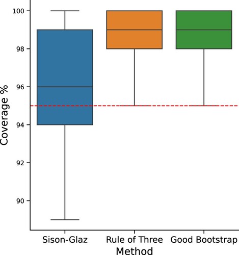
Figure 1 illustrates the log-volume of the examined SCIs for a sample size of n = 500 and an increasing alphabet size. As we can see, our proposed Good-Bootstrap scheme outperforms the alternatives for all the examined distributions and alphabet sizes. In addition, Figure 2 demonstrates the coverage of the three SCI schemes. As we can see, both the Good-Bootstrap and the ROT method maintain the desired confidence level, while SG fails to do so. This is not quite surprising, as discussed in Section 2. Additional examination of the SCIs coverage for larger experimental setting is provided in Appendix 2.

Next, we examine the obtained CI for different symbols in the alphabet. Figure 3 demonstrates the length of the CI for every symbol in the Zipf's Law experiment (s = 1.01). Importantly, notice that the greyed area corresponds to the collection of symbols which holds $95\mathrm{\%}$ of the probability mass. As expected, the Good-Bootstrap scheme outperforms both alternatives in this important region.

Figure 1. Simulation results for sample size of 500 and an increasing alphabet size, averaged over 100 trials. Each plot represents different distribution, Step distribution (upper left), Uniform (upper right), Zipf's Law with s = 1.01 (lower left), and Zipf's Law with s = 1.5 (lower right).

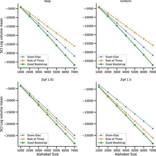
Figure 2. Coverage percentage of the different methods, out of 100 trials. The red dashed line indicates the desired coverage level.

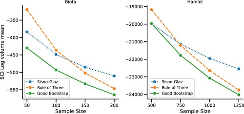
Finally, we proceed to real-world experiments. In Figure 4, we compare the performance of the three SCI schemes on real-world data. The Biota data-set consists of the frequency of 182 species-level operational taxonomic units (SLOTUs) similar to Gao et al. (2007). The Hamlet data-set consists of the frequency of approximately 5000 distinct words in the classical Hamlet play. Notice that in these real-world settings, the true underlying probability is unknown. Hence, the underlying distribution p refers to the total frequency of symbols, in the full data-set. We examine the three SCI schemes for different sample sizes. Similarly to the above, we compare their corresponding confidence region volumes and evaluate their coverage rate. As above, the Good-Bootstrap scheme demonstrate improved performance compared to the alternatives.

Figure 3. CI length of the different methods by log true probability of symbols in a zipf's Law experiment (s = 1.01).The Gray area corresponds to $95\mathrm{\%}$ percent of the total probability mass.

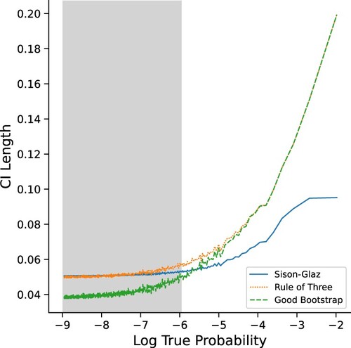
Figure 4. Real-world experiments. The Biota data-set is on the left and the Hamlet play on the right.

6. Discussion and conclusions

In this work we introduce a novel SCI scheme for large alphabet multinomial proportions. The proposed Good-Bootstrap scheme is based on a bootstrap statistic, $p_{\max }(X^n)=\underset{i}{max}\{p(i)\mid N_i=0\}$, which corresponds to the maximal probability over all the symbols that do not appear in the sample. This statistic is utilised to construct a CI for all the symbols that do not appear in the sample, while the remaining symbols are treated with a Bonferroni corrected binomial CI. We examine our proposed method on synthetic and real-world data, and show it outperforms popular alternatives in large alphabet regimes. We further show that the Good-Bootstrap maintains the desired coverage level, as expected.

The proposed inference scheme is easy to implement. Further, our experiments show that it is more computationally efficient than the SG algorithm. Although our algorithm is designed to address the unobserved symbols, it could be generalised to similarly address symbols that appear once, twice or more times in the sample. Another further improvement is the binomial treatment of the sampled symbols. Currently, we use the Clopper-Pearson method, which is considered conservative. Using a less conservative method may result in smaller confidence volumes while still maintaining the desired confidence level. We consider these directions for our future work.

Disclosure statement

No potential conflict of interest was reported by the author(s).

Additional information

Funding

This research is supported by the Israel Science Foundation [grant number 963/21].

Appendices

Appendix 1.

Exact bootstrap estimator

Given a sample $X^n$ and a distribution p, we introduce an exact analytical expression for (4(4) $P(p_{\max }(X^n)\le T(X^n))\ge 1-\delta ,$(4) ). Assume without loss of generality that the m symbols are sorted in a ascending order, according to their corresponding probabilities $p_i$. Then, we evaluate the distribution of $p_{\max }(X^n)$ as follows. (A1) $\begin{array}{rl}& P(p_{\max }(X^n)=p_i)=P(N_i=0,N_{i+1}>0,\dots ,N_m>0)\\ & =P(N_i=0)P(N_{i+1}>0|N_i=0)P(N_{i+2}>0|N_{i+1}>0,N_i=0)\cdots \\ & P(N_m>0|N_{m-1}>0,\dots ,N_i=0)\end{array}$(A1) Let us derive each of the terms above. First we have $P(N_i=0)=(1-p_i{)}^n$. Next, (A2) $P(N_j>0|N_i=0)=1-P(N_j=0|N_i=0)=1-{(1-\frac{p_j}{1-p_i})}^n$(A2) for every $j\ne i$. Similarly, we have (A3) $\begin{array}{rl}& P(N_j>0|N_i=0,N_t=0)=1-P(N_j=0|N_i=0,N_t=0)=1-{(1-\frac{p_j}{1-p_i-p_t})}^n,\end{array}$(A3) which we use for our following derivations. Further, (A4) $\begin{array}{rl}& P(N_w>0|N_j>0,N_i=0)\\ & =\sum _{k=1}^{n}P(N_w>0|N_j>0,N_i=0,N_j=k)\cdot P(N_j=k|N_j>0,N_i=0)\\ & =\sum _{k=1}^{n}P(N_w>0|N_i=0,N_j=k)\frac{P(N_j>0|N_j=k,N_i=0)P(N_j=k|N_i=0)}{P(N_j>0|N_i=0)}\\ & =\frac{1}{P(N_j>0|N_i=0)}\cdot \sum _{k=1}^{n}P(N_w>0|N_i=0,N_j=k)\cdot P(N_j=k|N_i=0)\\ & =\frac{P(N_w>0|N_i=0)-P(N_w>0|N_i=0,N_j=0)P(N_j=0|N_i=0)}{P(N_j>0|N_i=0)}\end{array}$(A4) where all the terms that are used in (A4(A4) $\begin{array}{rl}& P(N_w>0|N_j>0,N_i=0)\\ & =\sum _{k=1}^{n}P(N_w>0|N_j>0,N_i=0,N_j=k)\cdot P(N_j=k|N_j>0,N_i=0)\\ & =\sum _{k=1}^{n}P(N_w>0|N_i=0,N_j=k)\frac{P(N_j>0|N_j=k,N_i=0)P(N_j=k|N_i=0)}{P(N_j>0|N_i=0)}\\ & =\frac{1}{P(N_j>0|N_i=0)}\cdot \sum _{k=1}^{n}P(N_w>0|N_i=0,N_j=k)\cdot P(N_j=k|N_i=0)\\ & =\frac{P(N_w>0|N_i=0)-P(N_w>0|N_i=0,N_j=0)P(N_j=0|N_i=0)}{P(N_j>0|N_i=0)}\end{array}$(A4) ) may be evaluated according to (A3(A3) $\begin{array}{rl}& P(N_j>0|N_i=0,N_t=0)=1-P(N_j=0|N_i=0,N_t=0)=1-{(1-\frac{p_j}{1-p_i-p_t})}^n,\end{array}$(A3) ) and (A2(A2) $P(N_j>0|N_i=0)=1-P(N_j=0|N_i=0)=1-{(1-\frac{p_j}{1-p_i})}^n$(A2) ). This means we may compute each of the terms in (A1(A1) $\begin{array}{rl}& P(p_{\max }(X^n)=p_i)=P(N_i=0,N_{i+1}>0,\dots ,N_m>0)\\ & =P(N_i=0)P(N_{i+1}>0|N_i=0)P(N_{i+2}>0|N_{i+1}>0,N_i=0)\cdots \\ & P(N_m>0|N_{m-1}>0,\dots ,N_i=0)\end{array}$(A1) ) recursively, one after the other. That is, (A5) $\begin{array}{rl}& P(N_t>0|N_{t-1},\dots ,N_{t-l}>0,N_{t-l-1}=0)\\ & =\sum _{k=1}^{n}P(N_t>0|N_{t-1}=k,N_{t-2}>0,\dots ,N_{t-l}>0,N_{t-l-1}=0)\cdot \\ & P(N_{t-1}=k|N_{t-2}>0,\dots ,t-l>0,N_{t-l-1}=0)\\ & =\sum _{k=1}^{n}P(N_t>0|N_{t-1}=k,N_{t-2}>0,\dots ,N_{t-l}>0,N_{t-l-1}=0)\cdot \\ & P(N_{t-1}>0|N_{t-1}=k,N_{t-2}>0,\dots ,N_{t-l-1}=0)\cdot \\ & \frac{P(N_{t-1}=k|N_{t-2}>0,\dots ,N_{t-l-1}=0)}{P(N_{t-1}>0|N_{t-2}>0,\dots ,N_{t-l-1}=0)}\\ & =\frac{1}{P(N_{t-1}>0|N_{t-2}>0,\dots ,N_{t-l-1}=0)}\cdot \\ & \sum _{k=1}^{n}P(N_t>0|N_{t-1}=k,N_{t-2}>0,\dots ,N_{t-l-1}=0)\cdot \\ & P(N_{t-1}=k|N_{t-2}>0,\dots ,N_{t-l-1}=0)\\ & =\frac{1}{P(N_{t-1}>0|N_{t-2}>0,\dots ,N_{t-l-1}=0)}\cdot \\ & (P(N_t>0|N_{t-2}>0,\dots ,N_{t-l-1}=0)-\\ & P(N_t>0|N_{t-1}=0,N_{t-2}>0,\dots ,N_{t-l-1}=0)\cdot \\ & P(N_{t-1}=0|N_{t-2}>0,\dots ,N_{t-l-1}=0))\end{array}$(A5) where:

• $P(N_{t-1}>0|N_{t-2}>0,\dots ,N_{t-l-1}=0)$ and $P(N_t>0|N_{t-2}>0,\dots ,N_{t-l-1}=0)$ are evaluated according to the previous step.

• $P(N_t>0|N_{t-1}=0,N_{t-2}>0,\dots ,N_{t-l-1}=0)$ is similar to the previous expression, but since we are given that $N_{t-1}=0$, the conditional probability satisfies $1-(1-\frac{p_t}{1-p_{t-1}}{)}^n$ (as in A2(A2) $P(N_j>0|N_i=0)=1-P(N_j=0|N_i=0)=1-{(1-\frac{p_j}{1-p_i})}^n$(A2) ).

• $P(N_{t-1}=0|N_{t-2}>0,\dots ,N_{t-l-1}=0)=1-P(N_{t-1}>0|N_{t-2}>0,\dots ,N_{t-l-1}=0)$, which follows the derivation above.

Appendix 2.

Multiple experiments coverage

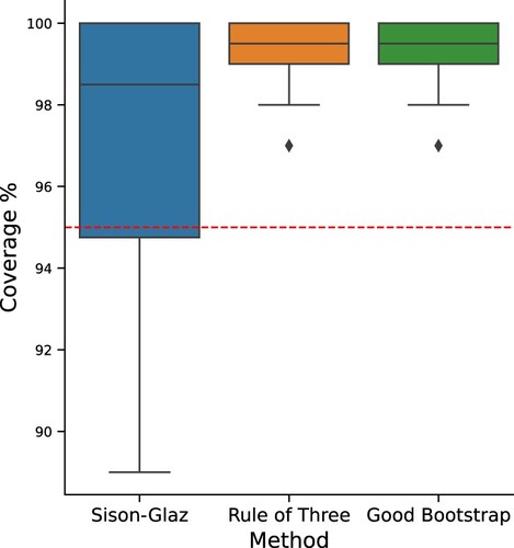
We report the accumulated coverage of the examined inference SCIs, over all of our synthetic experiments. That is, we record the coverage for each of our experiments (different values of n and m), and draw their accumulated box plots. We expect a 0.95 confidence level in all of our experiments. As we can see, both the ROT and our proposed method satisfy the above while SG fails to do so.

Figure A1. Coverage percentage of the different methods, out of 100 trials. Alphabet sizes of 100, 500, 1000, 5000, and sample sizes of 100, 500, 1000, 5000. Red line indicates the desired coverage level

References

- Benjamini, Y., Hechtlinger, Y., and Stark, P.B. (2019), 'Confidence Intervals for Selected Parameters', arXiv preprint arXiv:1906.00505.
- Carpenter, J., and Bithell, J. (2000), ‘Bootstrap Confidence Intervals: When, Which, What? A Practical Guide for Medical Statisticians’, Statistics in Medicine, 19(9), 1141–1164.
- Chafai, D., and Concordet, D. (2009), ‘Confidence Regions for the Multinomial Parameter with Small Sample Size’, Journal of the American Statistical Association, 104(487), 1071–1079.
- Clopper, C.J., and Pearson, E.S. (1934), ‘The Use of Confidence or Fiducial Limits Illustrated in the Case of the Binomial’, Biometrika, 26(4), 404–413.
- Efron, B., and Tibshirani, R.J. (1994), An Introduction to the Bootstrap. New York, NY: CRC Press.
- Fitzpatrick, S., and Scott, A. (1987), ‘Quick Simultaneous Confidence Intervals for Multinomial Proportions’, Journal of the American Statistical Association, 82(399), 875–878.
- Gale, W.A., and Sampson, G. (1995), ‘Good-Turing Frequency Estimation Without Tears’, Journal of Quantitative Linguistics, 2(3), 217–237.
- Gao, Z., Tseng, Ch., Pei, Z., and Blaser, M.J. (2007), ‘Molecular Analysis of Human Forearm Superficial Skin Bacterial Biota’, Proceedings of the National Academy of Sciences, 104(8), 2927–2932.
- Good, I.J. (1953), ‘The Population Frequencies of Species and the Estimation of Population Parameters’, Biometrika, 40(3–4), 237–264.
- Good, I.J. (2000), ‘Turing's Anticipation of Empirical Bayes in Connection with the Cryptanalysis of the Naval Enigma’, Journal of Statistical Computation and Simulation, 66(2), 101–111.
- Goodman, L.A. (1964), ‘Simultaneous Confidence Intervals for Contrasts among Multinomial Populations’, The Annals of Mathematical Statistics, 35(2), 716–725.
- Hesterberg, T.C. (2015), ‘What Teachers Should Know about the Bootstrap: Resampling in the Undergraduate Statistics Curriculum’, The American Statistician, 69(4), 371–386.
- Laplace, P.-S. (1825), Pierre-Simon Laplace Philosophical Essay on Probabilities: Translated from the Fifth French Edition of 1825 with Notes by the Translator, Vol. 13. New York, NY: Springer Science & Business Media.
- Malloy, M.L., Tripathy, A., and Nowak, R.D. (2020), ‘Optimal Confidence Regions for the Multinomial Parameter’, arXiv preprint arXiv:2002.01044.
- Mandel, M., and Betensky, R.A. (2008), ‘Simultaneous Confidence Intervals Based on the Percentile Bootstrap Approach’, Computational Statistics & Data Analysis, 52(4), 2158–2165.
- May, W.L., and Johnson, W.D. (1997), ‘Properties of Simultaneous Confidence Intervals for Multinomial Proportions’, Communications in Statistics – Simulation and Computation, 26(2), 495–518.
- McAllester, D.A., and Schapire, R.E. (2000), ‘On the Convergence Rate of Good-Turing Estimators’, in Colt, pp. 1–6.
- Nadas, A. (1985), ‘On Turing's Formula for Word Probabilities’, IEEE Transactions on Acoustics, Speech, and Signal Processing, 33(6), 1414–1416.
- Nowak, R., and Tánczos, E. (2019), ‘Tighter Confidence Intervals for Rating Systems’, arXiv preprint arXiv:1912.03528.
- Orlitsky, A., Santhanam, N.P., and Zhang, J. (2003), ‘Always Good Turing: Asymptotically Optimal Probability Estimation’, Science, 302(5644), 427–431.
- Orlitsky, A., and Suresh, A.T. (2015), ‘Competitive Distribution Estimation: Why is Good-Turing Good’, in Advances in Neural Information Processing Systems, pp. 2143–2151.
- Painsky, A. (2021), ‘Refined Convergence Rates of the Good-Turing Estimator’, in 2021 IEEE Information Theory Workshop (ITW), pp. 1–5.
- Painsky, A. (2022a), ‘A Data-Driven Missing Mass Estimation Framework’, in 2022 IEEE International Symposium on Information Theory (ISIT), pp. 2991–2995.
- Painsky, A. (2022b), ‘Generalized Good-Turing Improves Missing Mass Estimation’, Journal of the American Statistical Association, 1–10.
- Quesenberry, C.P., and Hurst, D. (1964), ‘Large Sample Simultaneous Confidence Intervals for Multinomial Proportions’, Technometrics, 6(2), 191–195.
- Saichev, A.I., Malevergne, Y., and Sornette, D. (2009), Theory of Zipf's Law and Beyond, Vol. 632. Berlin, Germany: Springer Science & Business Media.
- Sison, C.P., and Glaz, J. (1995), ‘Simultaneous Confidence Intervals and Sample Size Determination for Multinomial Proportions’, Journal of the American Statistical Association, 90(429), 366–369.
- Vysochanskij, D., and Petunin, Y.I. (1980), ‘Justification of the 3 Sigma Rule for Unimodal Distributions’, Theory of Probability and Mathematical Statistics, 21, 25–36.
- Zabell, S.L. (1989), ‘The Rule of Succession’, Erkenntnis, 31(2–3), 283–321.