
 ?Mathematical formulae have been encoded as MathML and are displayed in this HTML version using MathJax in order to improve their display. Uncheck the box to turn MathJax off. This feature requires Javascript. Click on a formula to zoom.
Abstract
In this paper, we are interested in nonparametric kernel estimation of a generalised regression function based on an incomplete sample copies of a continuous-time stationary and ergodic process
. The predictor X is valued in some infinite-dimensional space, whereas the real-valued process Y is observed when the Bernoulli process
and missing whenever
. Uniform almost sure consistency rate as well as the evaluation of the conditional bias and asymptotic mean square error are established. The asymptotic distribution of the estimator is provided with a discussion on its use in building asymptotic confidence intervals. To illustrate the performance of the proposed estimator, a first simulation is performed to compare the efficiency of discrete-time and continuous-time estimators. A second simulation is conducted to discuss the selection of the optimal sampling mesh in the continuous-time case. Then, a third simulation is considered to build asymptotic confidence intervals. An application to financial time series is used to study the performance of the proposed estimator in terms of point and interval prediction of the IBM asset price log-returns. Finally, a second application is introduced to discuss the usage of the initial estimator to impute missing household-level peak electricity demand.
1. Introduction
Let be an infinite-dimensional space equipped with a semi-metric
. Consider
a stationary and ergodic continuous-time process valued in the space
, such that each triplet
has the same probability distribution as the random variable (r.v.)
defined on probability space
. Let S be a compact interval in
and ψ be a measurable function defined on the space
,
, where y is a real variable such that
. Consider the following regression model:
(1)
(1)
where
is the conditional expectation of
given the r.v. X. That is, for any
and a fixed
,
. The error term ε is independent of X such
almost surely (a.s.)
Usually, when no data are missing, a sample of stationary and ergodic process is observed. Here, we allow the response variable
to be Missing At Random (MAR) any time t. To check whether an observation is complete or missing, a new variable ζ is introduced into the model as an indicator of the missing observations. Thus, for any
,
if
is observed and 0 if
is missing. We suppose that the Bernoulli random variable ζ satisfies
. Here,
is the conditional probability of observing the response variable and is usually unknown. This assumption allows to conclude that ζ and Y are conditionally independent given X. Note that the above assumption says that the response variable does not provide additional information, on top of that given by the explanatory variable, to predict whether an individual will present a missing response.
In this paper, we are interested in the estimation of the regression function based on the observed data
. Note that, for any
,
is an element in the space
, which means that, for any fixed time
,
is a curve. Specifically, if
is the space of square integrable functions defined on
, then the predictor
describes a trajectory in the functional space
observed at the fixed time
.
In real life, there are several situations where the response variable might be missing at random. For instance, in survey sampling studies the non-response is an increasingly common problem, where the missing response reaches rates of –
or even higher (see, e.g. Sikov Citation2018). In such cases, the missing data become a real source of bias in survey sampling estimation. Another case where the response may be subject to the MAR phenomena is the household electricity consumption monitoring. Indeed, the real-time collection of intra-day electricity consumption is now possible after the deployment of smart meters at the household level. The transmission of the information from the smart meter towards the information system goes usually through WIFI or optical fibre networks which are significantly dependent on the weather conditions, among other factors. Therefore, a response variable such as the daily total electricity consumption might be subject to missing at random mechanism due to bad weather conditions (for more details , see Section 5.2). In financial market, despite the modern technology, which allows to collect data at a very fine time scale, financial data can still be missing. For instance, there are some regular holidays, such as Thanksgiving Day and Christmas, for which stock price data are missing. There are many other technical reasons (such as breakdown in devises recording data, computers' sudden shutdowns, …) that make stretches of data missing (see Section 5.1 for more details about this application). For further examples and details about missing at random data the reader is referred to Chapter 1 in Little and Rubin (Citation2002).
Whenever is an independent and identically distributed (i.i.d) random sample several authors investigated nonparametric and semiparametric estimations of the regression function. In the framework where X is a finite dimensional, one can quote (Cheng Citation1994; Little and Rubin Citation2002; Nittner Citation2003; Tsiatis Citation2006; Liang et al. Citation2007; Efromovich Citation2011). See also, Ferraty et al. (Citation2013) when the predictor is infinite-dimensional. However, less attention has been given to the case of dependent data including an infinite-dimensional covariate, except Ling et al. (Citation2015), where a local constant estimation of the regression operator with discrete-time ergodic processes was considered.
In the case of continuous-time finite dimensional processes (d and
) satisfying a strong mixing condition, the estimation of the regression function based on completely observed data was considered by several authors, see for instance, the monograph by Bosq (Citation1998) and the references therein.
Some of these results were extended by Didi and Louani (Citation2014) and Bouzebda and Didi (Citation2017) for stationary and ergodic processes. Chaouch and Laïb (Citation2019) studied the asymptotic mean square error of the kernel regression estimator for MAR stationary and ergodic process and obtained an explicit upper bound of it.
It is worth noting that, even though a continuous-time functional processes framework is considered in this paper, in practice data are often collected according to some sampling scheme and the continuous-time process is discretised. Our results are then valid when considering a discrete-time ergodic stationary process sampled from a continuous-time process
with a regular sampling mesh
A discussion on the optimal choice of the sampling mesh in the continuous-time case will be then of great practical interest (see Section 3.5 and Simulation 2).
In the setting where is an α-mixing continuous-time process with Y is completely observed, Maillot (Citation2008) established the convergence with rates of the regression operator, and a super-optimal mean square convergence rate was obtained in Chesneau and Maillot (Citation2014).
This paper aims to complete and extend (Maillot Citation2008; Chesneau and Maillot Citation2014; Ling et al. Citation2015) work at several levels. First, we suppose that the continuous-time process satisfies an ergodic assumption rather than an α-mixing one. Therefore, the dependence structure considered here is more general and involves several processes which do not satisfy the mixing property. Indeed, our results are valid for α-mixing and non α-mixing as well as long memory and Bernoulli shift processes (for more details, see examples used to discuss Assumption A3 below). Moreover, our results are stated and proved without assuming neither mixing condition nor imposing a particular covariance structure on the process. This is due to the fact that the main technical tools used here are martingale difference devices and sequence of projections on appropriate σ-fields. Second, we complete and extend results established in Ling et al. (Citation2015) for discrete-time functional data processes, to the continuous-time functional framework.
We estimate a general operator which includes conditional mean, conditional distribution function and conditional quantiles. It is worth noting that such extension is not obvious since it requires an appropriate definition of σ-fields adapted to continuous-time context. Such adaptation is crucial when using martingale difference tools to establish asymptotic properties of the estimator. Third, the response variable considered here is affected by the MAR mechanism and therefore is not completely observed as in Maillot (Citation2008). Moreover, in contrast to Maillot (Citation2008) and Chesneau and Maillot (Citation2014), we do not limit our study to the mean square convergence, but we provide a more exhaustive inference on the regression operator estimator including pointwise and uniform almost sure convergence rate, identification of the limiting distribution of our estimator, and provide method to build confidence intervals. Fourth, simulation study is also carried out to investigate the selection of the ‘optimal’ sampling mesh, which is one of the most important topics in nonparametric estimation with continuous-time processes.
The rest of this paper is organised as follows. In Section 2, we present the framework adapted to continuous-time ergodic processes and introduce assumptions needed for establishing asymptotic results. The main asymptotic properties of the estimator are discussed in Section 3. An illustration of the performance of the proposed estimator is discussed through simulated data in Section 4. Section 5 is devoted to an application of the proposed estimator to financial time series. Section 6 discusses the application of our theoretical results to continuous-time conditional quantiles estimation. Finally technical proofs are given in the Appendix.
2. Framework and assumptions
To define the framework of our study, we need to introduce some definitions. Let be a continuous-time process defined on a probability space
and observed at any time
. For more details about the definition of continuous-time ergodic processes, the reader is referred to Didi and Louani (Citation2014). From now on, we consider
the filtration defined on
, that is
is an increasing sequence of sub-σ-algebras of
.
For a positive real number δ such that and
, consider the δ-partition
of the interval
. Furthermore, for t>0 and
, we define the following σ-fields:
(2)
(2)
If t<0 we take
the trivial σ-field. Note that, for any
and t>0, we have
. Moreover, for any
, such that
we have
.
Let be a ball centred at
with radius
Denote
a nonnegative real-valued continuous-time process and let
and
be the distribution function and conditional distribution function of
given the σ-field
, respectively.
To define an estimator of the regression function adapted to the MAR, multiply Equation (Equation1(1)
(1) ) by ζ to get
Taking conditional expectations with respect to X = x, one gets
Thus we have
Given a random sample
one can therefore define a kernel-type estimator of
, say
, adapted to the MAR response framework. Note that if there are missing observations in the response variable, a simple way to estimate
is to consider a kernel smoothing-type estimator which only considers observed data, in other words, those for which
. Therefore, one gets
(3)
(3)
where
,
is a kernel density function,
is the smoothing parameter tending to zero as T goes to infinity.
Remark 2.1
When the sample has missing observations in the response variable, two strategies can be followed to estimate . The first one,
given in Equation (Equation3
(3)
(3) ), called simplified estimator which only uses complete observations. The second approach consists in using the simplified estimator
to impute the missing values of the response variable
according to the following expression:
, (see, e.g. Chu and Cheng Citation2003 or González-Manteiga and Pérez-González Citation2004). Consequently, an estimator, say
, based on imputed data may be defined as follows:
From now on, we set and define the conditional bias as
(4)
(4)
where
and for
(5)
(5)
Before introducing the assumptions under which we establish our asymptotic results, we add the following notations. Let
denote a real random function ℓ such that
converges to zero almost surely (a.s.) as
and denote
a real random function ℓ such that
is almost surely bounded.
(Assumptions on the kernel function). Let K be a nonnegative bounded kernel of class
over its support
(Assumptions related to the continuous-time functional ergodic processes)
Let
Moreover, let
For any
For any
There exists a nondecreasing bounded function
(Local smoothness and continuity conditions)
Suppose for any
For any
The functions
For j = 1, 2, define the following moments, which are independent of
(6)
(6)
where
denotes the jth derivative of the kernel
and
the first derivative of K raised to the power j.
2.1. Comments on the assumptions
Condition (A1) is related to the choice of the kernel K, which is very usual in nonparametric functional estimation. Note that Parzen symmetric kernel is not adequate in this context since the random process is positive, therefore we consider K with support
. This is a natural generalisation of the assumption usually made on the kernel in the multivariate case where K is supposed to be a spherically symmetric density function. The assumptions
and
guarantee that
for all limit functions
In the case of non-smooth processes,
may be equal to the Dirac δ-function at 1, the condition
is needed to define the moments
which are, in this case, determined by the value
.
Conditions (A2)(i) –(ii) reflect the ergodicity property assumed on the continuous-time functional process. It plays an important role in studying the asymptotic properties of the estimator. The functions and f play the same role as the conditional and unconditional densities in finite dimensional case, whereas
characterises the impact of the radius u on the small ball probability as u goes to 0. Several examples to satisfy these conditions are given in Laïb and Louani (Citation2010) for discrete-time functional data process. Some other examples satisfying this condition are also given in Didi and Louani (Citation2014) when observations
are sampled from an ergodic continuous-time process taking values in
space.
Condition (A2)-(iii) involves the ergodic nature of the process where the random function belongs to the space of continuous functions. Note that approximating the integral
by its Riemann's sum:
allows to easily prove that the sequence
is stationary and ergodic (see Didi and Louani Citation2014). (A2)-(iv) is a usual condition when dealing with functional data, whereas (A2)-(v) is a consequence of ergodic assumption.
(A.3)(ii) is a Hölder-type assumption that requires a certain smoothness of the regression operator Such assumption is commonly used in nonparametric estimation. (A.3)(iii) is a smoothness condition on the κth centred conditional moments of
(A3)(iv) assumes the continuity of the conditional probability of observing a missing response. Finally, note that the moments
are linked to the small probability function through
. One can refer to Ferraty et al. (Citation2007) for a discussion on the choice of
, the Kernel K and the positively of
.
Discussion on the assumptions (A3)(i) –(i). These hypotheses are Markov-type conditions that characterise the conditional moments of
. They are satisfied for a general class of processes including the α-mixing and non α-mixing as well as long memory and the Bernoulli shift processes. As pointed in Doukhan and Louhichi (Citation1999), the main attraction of Bernoulli shift processes is that they provide examples of processes that are weakly dependent, but not mixing. According to the discussion made in the introduction we consider below some examples in both context (continuous and discretised processes) where the predictor X is a stationary and ergodic Markovian process that might be α-mixing or not and satisfies the conditions (A.3)(i) –(
).
First of all let us recall the following definitions.
Definition 2.1
see Doukhan and Louhichi (Citation1999)
Let be a sequence of independent real-valued r.v.s and F be a measurable function defined on
A Bernoulli shift is a sequence
defined by
Definition 2.2
see Doukhan (Citation2018, p. 60)
A centred second-order stationary process is called long-range dependent (LRD) if
and
, where
Definition 2.3
A process is called a fractional Brownian motion (fBm) with Hurst exponent
; if it is almost surely continuous, centred Gaussian process with covariance
Definition 2.4
see Lemma 4.2 in Maslowski and Pospíšil (Citation2008)
A strictly stationary centred Gaussian process is ergodic if
Example 2.5
Continuous-time long memory processes
Let and consider the Langevin equation with fBM noise
and initial condition
:
(7)
(7)
Then, for each
, the following Gaussian stationary Markovian fractional Ornstein–Uhlenbeck process
defined as
is the unique (a.s.) solution of (Equation7
(7)
(7) ) with initial condition
(for more details, see Section 2, p. 5, in Cheridito et al. Citation2003).
Note that for , the auto-covariance function of
is similar to that of the increments of
. Therefore,
is ergodic (by Definition 2.3) and exhibits long-range dependence as detailed in Theorem 2.3 and the discussion in the end of page 8 in Cheridito et al. (Citation2003).
Now, to check the condition (A.3)(i), consider the model:
Let
be the σ-field generated by
.
It follows that, for any ,
.
Since are Markovian then
almost surely. Thus condition (A.3)(i) is satisfied.
Example 2.6
Discrete-time processes
As discussed above, in real life we do not observe the process continuously at any time . We rather observe a discretised version of it based on some sampling scheme. The following examples are used to show that Assumption (A3)(i) is also satisfied for discretised processes as well.
(i) Long-memory discrete-time processes. Let be a white noise process with variance
, and let I and B be the identity operator and the backshift operator, respectively. Giraitis and Leipus (Citation1995) have proved (see Theorem 1 p. 55) that the k-factor Gegenbauer process
where
if
or
if
, for
, is long memory, stationary, causal and invertible and has the moving average representation. That is
with
On the other hand, Guégan and Ladoucette (Citation2001) have shown that, if is a Gaussian process, then the above process is not strong mixing whereas the moving average representation of
confirms that it is a stationary Gaussian and ergodic process.
(ii) The stationary solution of the linear Markov AR(1) process: , where
are independent symmetric Bernoulli random variables taking values
and 1, is not α-mixing (see Andrews Citation1984). However,
is a Markovian stationary and ergodic process.
(iii) Let be an i.i.d. sequence uniformly distributed on
, and set
, where the sequence
represents the decimals of
. The process
is stationary and admits the following AR(1) representation:
where
is a strong white noise. This process is not α-mixing (see Francq and Zakoïan Citation2010, Example A.3, p. 349), but it is ergodic.
To check the hypothesis (A3)(i) for Examples (i), (ii) and (iii), consider the regression model where
is a white noise process independent of
and define the σ-field:
. It is then easy to see that condition (A3)(i) is fulfilled. The discrete-time processes in examples (i)–(iii) are still valid for the regression model developed in Section 3.5 under the context of sampling schemes.
3. Main results
In this section, we investigate several asymptotic properties of the continuous-time generalised regression estimator. Some particular cases, related to specific choices of the function , including the conditional cumulative distribution function and the conditional quantiles will also be discussed.
3.1. Almost sure consistency rates
3.1.1. Pointwise consistency
The following theorem establishes an almost sure pointwise consistency rate of
Theorem 3.1
Pointwise consistency
Assume that (A1)–(A3) hold true and the following conditions are satisfied:
(8)
(8)
Then, for T sufficiently large, we have
(9)
(9)
The proof of Theorem 3.1 is detailed in the supplementary material in Chaouch and Laïb (Citation2023).
Remark 3.1
Theorem 3.1 generalises Theorem 1 of Laïb and Louani (Citation2011) established in the context of discrete-time stationary and ergodic processes, and Theorem 3.4 of Ferraty et al. (Citation2005) stated under a strong mixing assumption with completely observed response where the support of y is reduced to one point. Moreover, the function can decrease to zero at an exponential rate, whenever
goes to zero, therefore
should be chosen to decrease to zero at a logarithmic rate.
3.1.2. Uniform consistency
To establish the uniform consistency with rate of the regression operator, we need some additional definitions and assumptions that allow to express the uniform convergence rate as a function of the entropy number. Let and S be compact sets in
and
, respectively. Consider, for any
, the ϵ-covering number of the compact set
, say
, defined by
The number
measures how full is the class
. The finite set of points
is called an ϵ-net of
if
, where
is the ball, centred at
and of radius ϵ, with respect to the topology induced by the semi-metric
. The quantity
is called the Kolmogorov's ϵ-entropy of the set
that may be seen as a tool to measure the complexity of the subset
, in the sense that high entropy means that a large amount of information is needed to describe an element of
with an accuracy ϵ. Several examples of
covering special cases of functional processes are given in Ferraty et al. (Citation2010) and Laïb and Louani (Citation2011).
| (U0) | Assume that (A2) holds uniformly in the following sense:
| ||||
| (U1) | The kernel function K satisfies the following conditions:
| ||||
| (U2) | For | ||||
| (U3) | There exist | ||||
| (U4) | Let | ||||
Conditions in (U0) are standard in this context to get uniform consistency rate. Condition (U1) is usually used when we deal with nonparametric estimation for functional data, (U2) requires the existence of the moments up to order 2 of . (U3) is a regularity condition upon the function
which is necessary to obtain the uniform consistency result over the compact S. (U4) allows to cover the subset
with a finite number of balls and to express the convergence rate in terms of the Kolmogorov's entropy of this subset. Similar condition has been used in Ferraty et al. (Citation2010), where the authors have pointed out that, for a radius not too large, one requires the quantity
to be not too small and not too large. This condition seems to satisfy this exigence, since it implies that
goes to 0 for sufficiently large T. Examples given in Ferraty et al. (Citation2010) and Laïb and Louani (Citation2011) satisfy (U4).
Theorem 3.2 states uniform consistency rate of the Kernel regression estimator. It generalises Theorem 2 in Ferraty et al. (Citation2010) in the i.i.d. case and that in Laïb and Louani (Citation2011) established in the context of discrete-time stationary and ergodic processes with completely observed response.
Theorem 3.2
Uniform consistency
Assume (A1), (U0)–(U4), (A3) hold true. Moreover, suppose conditions in (Equation8(8)
(8) ) are satisfied and
(10)
(10)
Then we have
(11)
(11)
The proof of Theorem 3.2 is detailed in the supplementary material in Chaouch and Laïb (Citation2023).
3.2. Asymptotic conditional bias and risk evaluation
Before evaluating the conditional bias, let us introduce some additional notations. Consider for i = 1, 2, the following assumption:
(BC1) Recall that and, for any
, denote
Assume that the function
is differentiable at 0 and satisfies
and
for any
. This condition was introduced in Ferraty et al. (Citation2007) and used by Laïb and Louani (Citation2010) to evaluate the conditional bias. The introduction of
allows to make an integration with respect to the real random variable
rather than the couple of random variables
, where
being functional continuous random variable.
The following proposition gives asymptotic expression of the conditional bias term, which generalises Proposition 1 in Laïb and Louani (Citation2010) for discrete-time estimator to our setting. Its proof is similar to the one in the discrete-time framework and therefore is omitted.
Proposition 3.3
Conditional Bias
Under assumptions (A1)–(A3), (BC1) and conditions in (Equation8(8)
(8) ), we have
The next result gives an explicit expression of the asymptotic quadratic risk associated to the estimator .
Theorem 3.4
Quadratic risk
Suppose that Assumptions (A1)–(A3) hold true. Then, whenever and
, we have, for a fixed
, that
where
Remark 3.2
Note that, for sufficiently large T, the expression of MSE becomes
The mean squared error can be used as a theoretical guidance to select the ‘optimal’ bandwidth by minimising the quantity
3.3. Asymptotic normality
The following theorem establishes the asymptotic distribution of the estimator.
Theorem 3.5
Assume that conditions (A1)–(A3) are fulfilled. Suppose that, for β as defined in (A3)(ii), the following conditions hold true:
(12)
(12)
Then, for any
such that
we have
where
(13)
(13)
and
Note that the statement (Equation13(13)
(13) ) gives only an upper bound of the asymptotic variance
. The following proposition gives an estimate of
that will be needed to construct confidence intervals for the unknown operator
.
Proposition 3.6
Suppose conditions of Theorem 3.5 hold and , then
(14)
(14)
is a consistent estimator for
. The quantities
,
,
,
and
are empirical versions of
,
,
,
and
respectively.
and
are calculated by replacing
, given in (A2)(iv), by its empirical version
On the other hand
and
are given by
3.4. Continuous-time confidence intervals
Using the non-decreasing property of the cumulative standard Gaussian distribution function, the estimator , defined in (Equation14
(14)
(14) ), with the help of Proposition 3.6 and Theorem 3.5, the following corollary provides estimated confidence intervals for
at any x fixed.
Corollary 3.7
Assume conditions of Theorem 3.5 are fulfilled and the conditions in (Equation12(12)
(12) ) are replaced by
(15)
(15)
Then, for any
, the
confidence intervals for
are
(16)
(16)
where
is the αth quantile of the standard normal distribution.
These intervals are similar to those given in Remark 2 in Laïb and Louani (Citation2010) for discrete-time ergodic context with complete data, and those obtained in Ling et al. (Citation2015) for discrete-time stationary ergodic data with missing at random response.
3.5. Sampling schemes and computation of the confidence intervals
In the previous section, the process was supposed to be observable over . However, in practice the data are often collected according to a sampling scheme since it is difficult to observe a path continuously at any time t over the interval
. Hereafter, we briefly discuss the effect of a sampling scheme on the construction of confidence intervals for the regression function
. Assume that the data are sampled, either regularly, irregularly or even randomly, from an underlying continuous-time process at instants
. For a sake of simplicity, we consider here the case where the instants
are irregularly spaced, that is
Now, for
, we define the following increasing families of σ-algebra:
and
The purpose then consists in estimating
given the discrete-time ergodic stationary process
sampled from the underlying continuous-time process
. In case of a regular sampling scheme, that is
, the regression function is
and its estimator
defined in (Equation3
(3)
(3) ) becomes
(17)
(17)
Note that Theorem 3.5 holds for the estimate
when replacing T by
. The limiting law is a Gaussian random variable with mean zero and variance function
Making use of Corollary 3.7 and considering similar steps as in Laïb and Louani (Citation2010), it follows that, for any
, the
asymptotic confidence intervals of
are
(18)
(18)
where
is the quantile of standard normal distribution.
4. Simulation study
This section aims to discuss numerically some aspects related to continuous-time processes that might affect the quality of estimation of the operator . Here we consider
therefore
, where
is the conditional expectation of
given
The first simulation aims to compare the quality of estimation of
based on the continuous-time and discrete-time processes. In the second simulation, we discuss the choice of the ‘optimal’ sampling mesh δ in the case of continuous-time processes and assess its sensitivity to the missing at random mechanism. Finally, the third simulation discusses the effect of the MAR rate on the coverage rate and length of the estimated confidence intervals.
4.1. Simulation 1: continuous-time versus discrete-time estimators
In this first simulation, we try to compare the estimation of the regression operator when discrete- and continuous-time processes are considered. We want to know whether considering a continuous-time processes may improve the quality of the predictions or not. We suppose that the functional space endowed with its natural norm. The generation of continuous-time processes
is obtained by considering the following steps:
First, we simulate an Ornstein–Uhlenbeck (OU) process
Let
We consider that curves are sampled at 400 equispaced values in
To generate the real-valued process
Observe that the OU process is a real-valued continuous-time process (since dt tends to zero). The operator
has a role to transform each observation in the process
into a curve through the Legendre polynomials. In such way, the functional variable X is generated continuously as is the process
. Moreover, note that steps 1, 2 and 3 are devoted to simulate the continuous-time functional process
, whereas in step 4 the real-valued continuous-time process
is generated. A sample of 20 simulated curves is displayed in Figure (left) and an example of the real-valued process
is given in Figure (right).
Figure 1. Left: A sample of 20 simulated curves . Right: A realisation of the process
.
![Figure 1. Left: A sample of 20 simulated curves {Xt(s):s∈[−1,1]}. Right: A realisation of the process (Yt)t∈[0,200].](/cms/asset/49028c87-f208-4048-959c-58c839a3dc8a/gnst_a_2332686_f0001_oc.jpg)
Now, our purpose is to compare, in terms of estimation accuracy, the continuous-time estimator with the discrete-time one for different values of T = 50, 200, 1000 and several missing at random rates. It is worth noting that the continuous-time process is observed at every instant
, where
and
. However, the discrete-time process is observed only at the instants
As in Ferraty et al. (Citation2013) and Ling et al. (Citation2015), we consider that the missing at random mechanism is led by the following probability distribution:
(21)
(21)
where
, for
Now, we specify the tuning parameters on which depend our estimator given in (Equation3
(3)
(3) ). We choose the quadratic kernel defined as
and because curves are smooth enough we choose as semi-metric the
-norm of the second derivatives of the curves, that is for
,
(22)
(22)
We used the local cross-validation method on the κ-nearest neighbours introduced in Ferraty and Vieu (Citation2006) page 116 to select the optimal bandwidth for both discrete- and continuous-time regression estimators. The accuracy of the discrete- and continuous-time regression estimators is evaluated over M = 500 replications. The accuracy is measured, at each replication
, by using the squared errors
and
for the continuous-time and discrete-time estimators, respectively. Observe that the discrete-time estimator of the regression operator is defined as
To get a better idea about the variability of the errors, Table summarises the distribution of the squared errors (multiplied by )
and
. It shows that continuous-time regression estimator is more accurate than the discrete-time one. Moreover, when T increases the squared errors decrease faster when working with the continuous-time process.
Table 1. Summary statistics of for discrete- and continuous-time estimators of the regression function.
4.2. Simulation 2: optimal sampling mesh selection
The purpose of this simulation is to investigate another aspect related to continuous-time processes. The selection of the ‘optimal’ sampling mesh is one of the most important topics in continuous-time processes.
First of all, we generate a continuous-time functional data process according to the following equation:
where
is an OU process solution of the stochastic differential equation (Equation19
(19)
(19) ) and practically observed at the instants
with n = 200 fixed. Here, we take different values of sampling mesh δ, calculate the corresponding empirical version of the Mean Integrated Square Error (
) and identify the optimal mesh, say
, that minimises
. Note that each curve observed at the instant t is discretised at 100 equidistant points over the interval
The response variable is obtained following the hereafter nonlinear functional regression model (Equation20
(20)
(20) ), where the operator
is defined as
Moreover, the missing at random mechanism in this simulation is also supposed to be the same as described in the first simulation as per Equation (Equation21
(21)
(21) ). For the tuning parameters used to build the estimator, we considered the quadratic kernel and given the shape of the true regression operator, which depends on the first derivative of the functional predictor, the Euclidean distance between the first-order derivatives of the curves is adopted as a semi-metric. Finally the bandwidth is selected according to the local cross-validation method based on the κ-nearest neighbours as detailed in Ferraty and Vieu (Citation2006, p. 116).
For each value of sampling mesh δ, the regression operator is estimated over a grid of 50 different fixed curves and the whole procedure is repeated over M = 500 replications. Finally, the empirical MISE is calculated, for each sampling mesh δ, according to the following equation:
Observe that
is the estimator of
, obtained at the kth iteration, depends on the sampling mesh δ, so is the MISE.
Figure displays the values of obtained for different values of sampling mesh δ and missing at random rate of 10%, 50% and 0% (complete data), respectively. One can observe that higher is the missing at random rate, higher are the errors in estimating the regression operator.
Figure 2. The obtained for different values of sampling mesh δ and several missing at random rates.
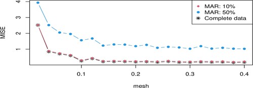
Table reports the optimal sampling mesh , which minimises
, for different missing at random rates. It also provides some summary statistics to have an idea about the distribution of
for several values of δ. One can observe, from Table , that higher is the missing at random rate longer we need to observe the underlying process to collect the n = 200 observations to be able to reasonably estimate the regression operator. Indeed, when the data is complete the optimal time interval
. However, when
(resp. 50%) the optimal time interval is equal to
(resp.
). Consequently, it can be concluded that when the missing at random mechanism is heavily affecting the response variable, we need to collect data over a longer period of time. This allows to get sufficient information about the dynamic of the underlying continuous-time process and therefore get a better estimate of the regression operator.
Table 2. The optimal sampling mesh () obtained for different MAR rates and some summary statistics of the MISE(δ).
4.3. Simulation 3: asymptotic confidence intervals
In this section, we are interested in evaluating the coverage rate, as well as the length, of the asymptotic confidence intervals given in (Equation16(16)
(16) ). The effect of the sampling mesh on the coverage rate will also be discussed numerically. Since this paper aims to extend results in Delsol (Citation2009) about confidence intervals to continuous-time functional data, we consider the same simulation framework.
Let where
is an OU process solution of the stochastic differential equation (Equation19
(19)
(19) ) observed at the instants
with n = 100, 200 fixed. Here, for comparison purpose, we consider two sampling mesh
The regression operator is defined as
, while the errors
are independent centred normal random variable with variance
, where
is the empirical variance of
Because the regression operator is defined as a function of the derivative of the functional random variable, the appropriate semimetric to be used in such case is based on the first derivative of the curve (see (Equation22
(22)
(22) )). Moreover, the quadratic kernel is used to perform this simulation. The optimal bandwidth is selected based on local cross-validation method on the κ-nearest neighbours. The missing at random rate is simulated according the conditional probability distribution given in (Equation21
(21)
(21) ).
For a fixed , the asymptotic
-confidence intervals for
with
are computed and compared for several values of sample size n and sampling mesh δ. Here
is a grid of
independently simulated curves where the regression operator is estimated. For every fixed curve
a number of M = 500 replications is considered to approximate the coverage rate. In this simulation
were considered.
As expected, Table shows that the average coverage rate varies with the sample size n, the sampling mesh and the MAR Rate. Higher are the sample size and the sampling mesh and smaller is the MAR rate closer will be the average coverage rate to Moreover, one can also observe that the asymptotic confidence intervals length decreases when the sample size increases and the MAR rate decreases.
Table 3. Average coverage over the grid Ξ and average confidence interval length appears in brackets.
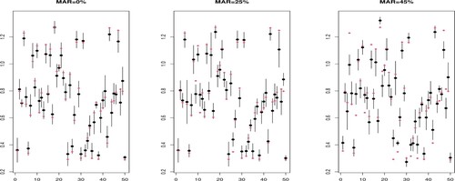
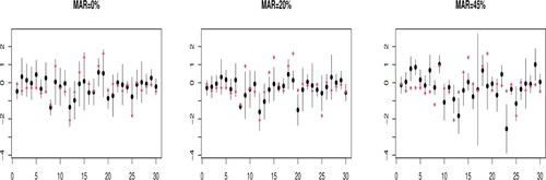
Figure (resp. Figure ) displays an example of asymptotic confidence intervals obtained for the 50 curves in the testing sample when n = 100, the MAR rate = 0%, 25%, 45%, and
(resp.
). One can observe that the coverage rate decreases with an increase in the MAR rate. Similar results are also obtained when
.
Figure 3. Asymptotic confidence intervals when
and n = 100. Red dot represents the true regression function value at any fixed curve
and the black dot is its estimation. The vertical lines represent the confidence intervals.
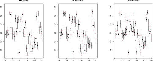
Figure 4. Asymptotic confidence intervals when
and n = 100. Red dot represents the true regression function value at any fixed curve
and the black dot is its estimation. The vertical lines represent the confidence intervals.
5. Applications to real data
5.1. Application 1: prediction of financial asset returns
In Financial market, despite the modern technology, which allows to collect data at a very fine time scale, financial data can still be missing. For instance, there are some regular holidays, such as Thanksgiving Day and Christmas, for which stock price data are missing. There are many other technical reasons (such as breakdown in devises recording data, computers' sudden shutdowns, …) that make stretches of data missing.
This section aims to assess the performance of the estimator proposed in this paper on missing at random financial functional time series. The International Business Machine cooperation (IBM) asset price is considered as the response variable and the Standard & Poor's 500 (SP500) stock market index as predictor. While the IBM asset price is observed at a daily frequency from 24 March 2016 to 28 September 2016, the SP500 is observed every minute during the same period. Note that the daily trading activity lasts for 7 hours excluding the weekend. Since in this paper, we are interested in stationary processes, a first-order differentiation of the IBM daily asset price and the SP500 stock market index was considered to make the original time series stationary.
Our sample here can be denoted as follows: , where the sample size n = 129 is the total number of trading days from 24 March 2016 to 28 September 2016 after first differentiation of the original time series,
,
Originally, the data are completely observed. Therefore, to validate our estimator, we artificially create missing observations. We assume here that the missing data are generated according to the conditional probability distribution given in (Equation21
(21)
(21) ). We split the original sample into training and testing subsets. Our purpose then is to predict the IBM asset price in the testing subset using the regression operator. Three MAR rates
(complete data),
and
were considered to test the performance of the estimator in terms of prediction. Similarly, as in the simulation section, we considered here the quadratic kernel and the bandwidth was selected using the cross-validation method on the κ-nearest neighbours. For the semi-metric, because the curves are not smooth (as it can be seen in Figure , right panel) we use the PCA-semi-metric, say
, based on the projection on the four eigenfunctions,
, associated to the four largest eigenvalues of the empirical covariance operator of the functional predictor X:
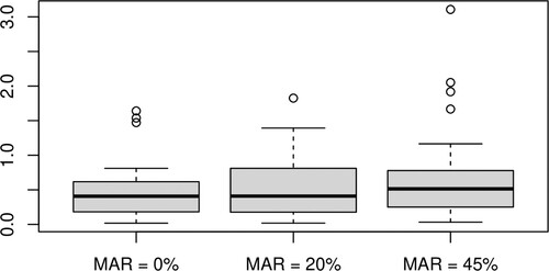
As criteria to measure the accuracy of the estimator in predicting 30 observations in the testing subset, we considered the Absolute Error:
for
. Figure displays the distribution of the absolute errors obtained when MAR rate is
and
, respectively. One can clearly observe the effect of the MAR rate on the quality of the prediction. Higher is the MAR rate lower is the quality of prediction.
Figure 5. Left: First-order differentiated IBM asset price. Right: First-order differentiated SP500 intraday (minute frequency) stock market index curves.
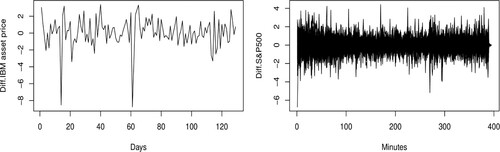
Figure 6. The obtained for different values of missing at random rates.
Moreover, we build a 95% prediction interval for the IBM asset price in the testing subset. Figure shows that the coverage rate is sensitive to the percentage MAR data in the training subset.
Figure 7. A 95% prediction interval of the IBM asset price in the testing subset. Red dot represents the true values of IBM asset price and the black dot is their prediction using the regression operator. The vertical lines represent the prediction intervals.
5.2. Application 2: Daily peak electricity demand imputation
By accurately predicting household peak load, utility companies can better balance the overall electricity demand and supply. This information helps in optimising power generation and distribution, ensuring a stable and reliable electricity grid. It also allows to plan for peak demand periods and avoid potential blackouts or overloading of the grid. Moreover, predicting peak loads empowers consumers with information about their electricity consumption patterns. Thus, with this knowledge, households can make informed decisions to manage their energy usage more effectively, reduce electricity bills and contribute to energy conservation efforts. Furthermore, peak load predictions enable demand response programs, where utility companies offer incentives for consumers to adjust their energy consumption during peak periods, thereby reducing strain on the grid.
For these reasons, electricity companies deployed smart meters to replace the mechanical one. This new generation of smart meters allows to record the electricity demand of any household at very fine time scale and send it to the information system. The transmission of the information from the smart meter towards the information system goes usually through WIFI or optical fibre networks which are significantly dependent on the weather conditions, among several other factors. Therefore, the calculation of the daily peak electricity demand might be subject to missing at random mechanism due to bad weather conditions.
Figure 8. Daily peak electricity demand of a household containing 10% missing data.
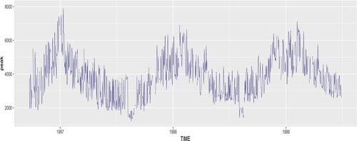
Figure 9. Intraday temperature curves. Coloured curves are for the missing peak load days.
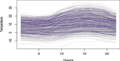
Figure 10. Daily peak electricity demand process. Red dots represent values of imputed missing data.
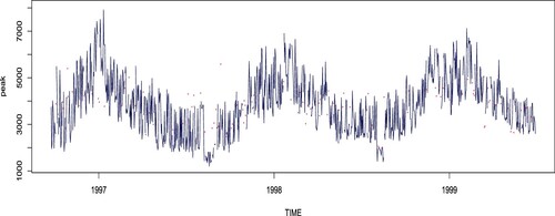
Figure 11. 95% confidence intervals for the imputed values.
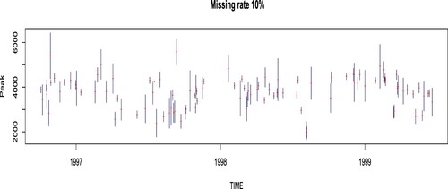
Figure displays the daily peak load obtained from a household smart meter from 24 September 1996 to 29 June 1999 (leading to a total of n = 1009 days). The original data contains 10% of missing observations. Here, we assume that the intraday (3-hour frequency) temperature curve
explains the missingness mechanism in the daily peak demand. Figure displays the intraday, 3-hour frequency, temperature curves. Our purpose in this application is to impute the missing data in the peak demand process using the initial estimator of the regression operator
defined in (Equation17
(17)
(17) ) with
Figure displays the imputed peak electricity demand process obtained according to the following formula:
If
is observed (that is
), then
, otherwise
is missing (i.e.
) and will be imputed by
The red dots in Figure represent the imputed values of the missing observations in the peak electricity demand process. Figure shows the 95% confidence intervals around the missing values of the peak load.
6. Discussion of a special case: conditional quantiles
Let be fixed and
, then if
the operator
is the conditional cumulative distribution function (df) of Y given X = x, namely
which may be estimated by
For a given
the
-order conditional quantile of the distribution of Y given X = x is defined as
Notice that, whenever is strictly increasing and continuous in a neighbourhood of
, the function
has a unique quantile of order α at a point
, that is
In such case
which may be estimated uniquely by
. Conditional quantiles have been widely studied in the literature when the predictor X is of finite dimension, see for instance, Gannoun et al. (Citation2003) and Ferraty et al. (Citation2005) for dependent functional data.
(a) Almost sure pointwise and uniform convergence
Under the same conditions of Theorem 3.1, the statement (Equation9(9)
(9) ) still holds for the estimator of the cumulative conditional distribution function
. That is
converges, almost surely, towards
with a rate
Consequently, since and
is continuous and strictly increasing, then we have
which implies that,
(23)
(23)
Therefore, the statement (Equation9
(9)
(9) ) still holds for the conditional quantile estimator
whenever conditions of Theorem 3.1 are satisfied. Ferraty et al. (Citation2005) derived similar pointwise convergence rate by inverting the estimator of the conditional cumulative distribution function. Their result has been obtained under mixing condition and additional assumptions on the joint distribution, and the Lipschitz condition on
and its derivatives with respect to y.
Regarding the almost sure uniform convergence, observe that under conditions of Theorem 3.2, the statement (Equation11(11)
(11) ) still holds true for the
, when
is replaced by
. Moreover, assume that, for fixed
,
is differentiable at
with
, where ν is a real number, and
is uniformly continuous for all
. Knowing that
and making use of a Taylor's expansion of the function
around
, we can write
(24)
(24)
where
lies between
and
. It follows then from (Equation24
(24)
(24) ) that the inequality (Equation23
(23)
(23) ) still holds true uniformly in x and y. Moreover, the fact that
converges a.s. towards
as T goes to infinity, combined with the uniformly continuity of
, allow to write that
(25)
(25)
Since
is uniformly bounded from below, we can then claim that the estimator
converges uniformly towards
with the same convergence rate given in (Equation11
(11)
(11) ), as T goes to infinity.
(b) Continuous-time confidence intervals
Confidence intervals for the conditional quantiles may be obtained according to the following steps. First, consider a Taylor's expansion of
around
and making use of the fact that
converges a.s. towards
as T goes to infinity, one gets
(26)
(26)
where
is a consistent estimator of
. Then, replacing
by the indicator function, we get under conditions of Corollary 3.7, the following
confidence intervals for
(27)
(27)
Supplemental Material
Download PDF (340.9 KB)Acknowledgments
Open Access funding provided by the Qatar National Library.
We thank the editor, associate editor and the two referees for their valuable and constructive comments which helped improve the manuscript substantially.
Disclosure statement
No potential conflict of interest was reported by the author(s).
Notes
1 For any such that
, there exists a non-negative continuous random function
such that
where
is a deterministic function.
References
- Andrews, D.W.K. (1984), ‘Non-strong Mixing Autoregressive Processes’, Journal of Applied Probability, 21, 930–934.
- Bosq, D. (1998), Nonparametric Statistics for Stochastic Processes: Estimation and Prediction, Lecture Notes in Statistics, Vol. 110 (2nd ed.), New York: Springer-Verlag.
- Bouzebda, S., and Didi, S. (2017), ‘Asymptotic Results in Additive Regression Model for Strictly and Ergodic Continuous Times Processes’, Communications in Statistics-Theory and Methods, 46(5), 2454–2493.
- Chaouch, M., and Laïb, N. (2019), ‘Optimal Asymptotic MSE of Kernel Regression Estimate for Continuous Time Processes with Missing At Random Response’, Statistics and Probability Letters, 154, 108532.
- Chaouch, M., and Laïb, N. (2023), ‘Supplement to “Regression estimation for continuous time functional data processes with missing at random response”’.
- Cheng, P.E. (1994), ‘Nonparametric Estimation of Mean Functionals with Data Missing at Random’, Journal of the American Statistical Association, 89, 81–87.
- Cheridito, P., Kawaguchi, H., and Maejima, M. (2003), ‘Fractional Ornstein–Uhlenbeck Processes’, Electronic Journal of Probability, 8(3), 1–14.
- Chesneau, C, and Maillot, B. (2014), ‘Superoptimal Rate of Convergence in Nonparametric Estimation for Functional Valued Processes’, International Scholarly Research Notices, 2014, 264217.
- Chu, C.K., and Cheng, P.E. (2003), ‘Nonparametric Regression Estimation with Missing Data’, Journal of Statistical Planning and Inference, 48, 85–99.
- de la Peña, V.H., and Giné, E. (1999), Decoupling: From Dependence to Independence, Probability and Its Applications, New York: Springer-Verlag.
- Delsol, L. (2009), ‘Advances on Asymptotic Normality in Non-parametric Functional Time Series Analysis’, Statistics, 43, 13–33.
- Didi, S., and Louani, D. (2014), ‘Asymptotic Results for the Regression Function Estimate on Continuous Time Stationary Ergodic Data’, Journal Statistics & Risk Modeling, 31(2), 129–150.
- Doukhan, P. (2018), Stochastic Models for Time Series, New York: Springer.
- Doukhan, P., and Louhichi, S. (1999), ‘A New Weak Dependence Condition and Applications to Moment Inequalities’, Stochastic Processes and Their Applications, 84, 313–342.
- Efromovich, S. (2011), ‘Nonparametric Regression with Responses Missing at Random’, Journal of Statistical Planning and Inference, 141, 3744–3752.
- Ferraty, F., Laksaci, A., Tadj, A., and Vieu, P. (2010), ‘Rate of Uniform Consistency for Nonparametric Estimates with Functional Variables’, Journal of Statistical Planning and Inference, 140, 335–352.
- Ferraty, F., Mas, A., and Vieu, P. (2007), ‘Nonparametric Regression on Functional Data: Inference and Practical Aspects’, Australian & New Zealand Journal of Statistics, 49(3), 267–286.
- Ferraty, F., Rabhi, A., and Vieu, P. (2005), ‘Special Issue on Quantile Regression and Related Methods’, Sankhyà : The Indian Journal of Statistics, 67(2), 378–398.
- Ferraty, F., Sued, M., and Vieu, P. (2013), ‘Mean Estimation with Data Missing at Random for Functional Covariables’, Statistics, 47(4), 688–706.
- Ferraty, F, and Vieu, P. (2006), Nonparametric Modelling for Functional Data, Methods, Theory, Applications and Implementations, London: Springer-Verlag.
- Francq, C., and Zakoïan, J.M. (2010), GARCH Models: Structure, Statistical Inference and Financial Applications, John Wiley and Sons Ltd.
- Gannoun, A., Saracco, J., and Yu, K. (2003), ‘Nonparametric Prediction by Conditional Median and Quantiles’, Journal of Statistical Planning and Inference, 117, 207–223.
- Giraitis, L., and Leipus, R. (1995), ‘A Generalized Fractionally Differencing Approach in Long-memory Modeling’, Lithuanian Mathematical Journal, 35(1), 53–65.
- González-Manteiga, W., and Pérez-González, A. (2004), ‘Nonparametric Mean Estimation with Missing Data’, Communications in Statistics-Theory and Methods, 33(2), 277–303.
- Guégan, D., and Ladoucette, S. (2001), ‘Non-mixing Properties of Long Memory Processes’, Comptes Rendus De L'Académie Des Sciences – Series I – Mathematics, 333(1), 373–376.
- Hall, P., and Heyde, C. (1980), Martingale Limit Theory and Its Application, New York: Academic Press.
- Laïb, N., and Louani, D. (2010), ‘Nonparametric Kernel Regression Estimation for Functional Stationary Ergodic Data: Asymptotic Properties’, Journal of Multivariate Analysis, 101(10), 2266–2281.
- Laïb, N., and Louani, D. (2011), ‘Rates of Strong Consistencies of the Regression Function Estimator for Functional Stationary Ergodic Data’, Journal of Statistical Planning and Inference, 141(1), 359–372.
- Liang, H., Wang, S., and Carroll, R.J. (2007), ‘Partially Linear Models with Missing Response Variables and Error-prone Covariates’, Biometrika, 94(1), 185–198.
- Ling, N., Liang, L., and Vieu, P. (2015), ‘Nonparametric Regression Estimation for Functional Stationary Ergodic Data with Missing At Random’, Journal of Statistical Planning and Inference, 162, 75–87.
- Little, R.J.A., and Rubin, D.B. (2002), Statistical Analysis with Missing Data (2nd ed.), New York: John Wiley.
- Maillot, B. (2008), ‘Propriétś Asymptotiques de Quelques Estimateurs Non-paramétriques Pour des Variables Vectorielles et Fonctionnelles’, Thése de Doctorat de l'Université Paris 6.
- Maslowski, B., and Pospíšil, P. (2008), ‘Ergodicity and Parameter Estimates for Infinite-dimensional Fractional Ornstein–Uhlenbeck Process’, Applied Mathematics and Optimization, 57, 401–429.
- Nittner, T. (2003), ‘Missing At Random (MAR) in Nonparametric Regression, a Simulation Experiment’, Statistical Methods and Applications, 12, 195–210.
- Sikov, A. (2018), ‘A Brief Review of Approaches to Non-ignorable Non-response’, International Statistical Review, 86, 415–441.
- Tsiatis, A. (2006), Semiparametric Theory and Missing Data, New York: Springer.
Appendix. Proofs of main results
In this section and for sake of simplification will denote and
for
and
, respectively, and
for
. Consider now the following quantities:
(A1)
(A1)
(A2)
(A2)
We have then
(A3)
(A3)
We start first by stating some technical lemmas that will be used later.
Lemma A.1
Assume that assumptions (A1)–(A2) are satisfied, then we have for any and
Proof.
The proof is similar to the proof of Lemma 1 of Laïb and Louani (Citation2010).
Lemma A.2
Let be a sequence of real martingale differences with respect to the sequence of σ-fields
where
is the sigma-field generated by the random variables
. Set
For any
and any
, assume that there exist some nonnegative constants C and
such that
almost surely. Then, for any
we have
where
Proof.
See Theorem 8.2.2 of de la Peña and Giné (Citation1999).
Proof
Proof of Theorem 3.4
From (EquationA3(A3)
(A3) ) and Lemma 1.2 (in Chaouch and Laïb Citation2023), we have for T large enough
(A4)
(A4)
where the products
and
have been ignored because by the Cauchz–Schwarz inequality
We have the same inequality for the second product. The proof of Theorem 3.4 results from Proposition 3.3 and Lemma A.3 below, which gives an upper bound of the expectation of
and
, respectively.
Lemma A.3
Assume that (A1)–(A3) hold true, then we have
(A5)
(A5)
Proof.
Ignoring the product term as above, one may write
The terms
and
can be handled similarly. Let us now evaluate the first one. Since
is a δ-partition of
, we have
(A6)
(A6)
Since
is a sequence of martingale differences with respect to the family
, then
for every
such that
Therefore (by ignoring the product term), we have
(A7)
(A7)
Using Jensen inequality and a double conditioning with respect to
combined with (A3)(iii) –(iv),
may bounded as
Similarly, we have
Therefore
Moreover, using the decomposition (EquationA2
(A2)
(A2) ), Theorem 3.3 and Lemma 1.1 (in Chaouch and Laïb Citation2023) one can see that
is negligible with respect to
This completes the proof.
Proof
Proof of Theorem 3.5
The proof of Theorem 3.5 is based essentially on Lemma A.4 established below, which gives the normality asymptotic of the principal term in (EquationA3
(A3)
(A3) ). Indeed, we have from (EquationA3
(A3)
(A3) ) that
(A8)
(A8)
Under (A1)–(A3), Lemma 1.2 (in Chaouch and Laïb Citation2023) implies that
converges, almost surely, to
as
Moreover, using Lemma 1.3 (in Chaouch and Laïb Citation2023), we get under (A3)(i) –(ii) combined with conditions (Equation12
(12)
(12) ) that
and
The proof may be then achieved by Lemma A.4 and Slutsky's Theorem.
Lemma A.4
Under conditions (A1)–(A3), we have
Proof
Proof of Lemma A.4
We have
(A9)
(A9)
Since for any
and
,
, then
is
-measurable,
provided
and
. Moreover, we have for any
,
a.s. Hence
is a sequence of martingale differences with respect to the σ-fields
. To prove the asymptotic normality, it suffices to check both following conditions (see Corollary 3.1, p. 56, Hall and Heyde Citation1980):
(a) and (b)
holds for any
.
Proof of (a) Observe now that
Using (A1), (A3)(i),(i
), (ii) and (iv) with Lemma A.1, and a double conditioning with respect to the σ-field
and the fact that
, we have
It follows by (A2)-(iii) and the Cauchy–Schwarz inequality that
Thus we have only to show that
. Using again the Cauchy–Schwarz inequality, one may write
(A10)
(A10)
Now, let us evaluate the term
. Conditioning three times with respect to
and
, and making use of Conditions (A3)(i
), (iii), (iv) and the fact that
, to get from Lemma A.1 that
(A11)
(A11)
The Riemann's sum combined with condition (A2)(iii) gives that
Moreover, by (A2)(ii) one gets
. Therefore, we have
(A12)
(A12)
On the other hand, by the same arguments as above combined with the fact that
, we get
.
Proof of part (b) Using successively Hölder, Markov, Jensen and Minkowski inequalities combined with conditions (A3)(iii), (A3)(iv) and Lemma A.1, we get, for any and fixed real numbers p>1 and q>1 such that
,
by taking
(
), since
towards to infinity as T goes to infinity.
Proof
Proof of Corollary 3.7
Observe that (A13)
(A13)
It follows from the consistency of
and (A2)(i) that
goes to 1 a.s. as T goes to infinity. By Theorem 3.5, the quantity
converges to
as
. Then using the non-decreasing property of the cumulative standard normal distribution function Ψ, we get, for a given risk
, the
- pseudo-confidence interval
(A14)
(A14)
Considering now the statement (Equation13
(13)
(13) ) combined with Proposition 3.6, it holds that
(A15)
(A15)
since
is a consistent estimator of
. The proofs follows then from the statements (EquationA13
(A13)
(A13) ), (EquationA14
(A14)
(A14) ) and (EquationA15
(A15)
(A15) ).