Process-Based psychotherapy personalization: considering causality with continuous-time dynamic modeling

ABSTRACT

Objective:

Psychotherapy can be improved by integrating the study of mediators (how it works) and moderators (for whom it works). To demonstrate this integration, we studied the relationship between resource activation, problem-coping experiences and symptoms in cognitive-behavior therapy (CBT) for depression, to obtain preliminary insights on causal inference (which process leads to symptom improvement?) and prediction (which one for whom?).

Method:

A sample of 715 patients with depression who received CBT was analyzed. Hierarchical Bayesian continuous time dynamic modeling was used to study the temporal dynamics between the variables analyzed within the first ten sessions. Depression and self-efficacy at baseline were examined as predictors of these dynamics.

Results:

There were significant cross-effects between the processes studied. Under typical assumptions, resource activation had a significant effect on symptom improvement. Problem-coping experience had a significant effect on resource activation. Depression and self-efficacy moderated these effects. However, when system noise was considered, these effects may be affected by other processes.

Conclusion:

Resource activation was strongly associated with symptom improvement. To the extent of inferring causality, for patients with mild-moderate depression and high self-efficacy, promoting resource activation can be recommended. For patients with severe depression and low self-efficacy, promoting problem-coping experiences can be recommended.

Keywords:

• process-outcome research
• prediction
• resource activation
• problem coping
• complex dynamic systems

Clinical and Methodological Significance of this Article: Based on patients’ depression severity and self-efficacy, intervention strategies can be recommended: Emphasizing either problem coping experiences or resource activation. The incorporation of a modeling approach such as continuous time dynamic modeling, contributes to the integration of studying mediators (therapeutic processes) and moderators (individual differences) into psychotherapy research.

Process-Based Psychotherapy Personalization:

Considering Causality with Continuous-Time Dynamic Modeling

Psychotherapy is an efficacious and effective treatment for common mental health problems (Barkham & Lambert, 2021). However, although numerous therapeutic approaches and new psychological interventions have emerged over the decades, psychotherapy outcomes have not improved (Wampold & Imel, 2015). For instance, in psychotherapy for depression, partial remission, relapse, and recurrences remain common phenomena (Cuijpers et al., 2021).

We can consider two general paths to improve the effectiveness of psychotherapy: identifying moderators (predictors) to find out for whom it works and identifying mediators to find out how it works (Huibers et al., 2021). The former is addressed by psychotherapy personalization research, while the latter by process-outcome studies. Psychotherapy personalization research develops models to recommend the right psychological treatment for the right individual at the right time (Cohen et al., 2021). In contrast, process-outcome studies identify phenomena occurring during psychotherapy that explain change, i.e., the therapeutic processes¹ that lead to a specific outcome (Crits-Christoph et al., 2021).

We agree with Huibers et al. (2021) that these two research lines should be integrated to move the field forward. Thus, answering not only for whom does it work? but how? This implies developing models that target specific psychotherapy processes and their relationship with treatment outcome, and allowing patients’ characteristics to moderate the relationships implied by the model (i.e., process-based psychotherapy personalization). However, causal inference needs to be addressed to ensure that the targeted processes for the particular patient are actually those responsible for outcome improvement. In the context of a process-based psychotherapy personalization, neglecting causal inference would lead to inaccurate identification of processes, compromising the effectiveness and precision of personalized psychotherapeutic interventions.

In psychology and psychotherapy research, causal inference constitutes a complex matter. On the one hand, there is a “taboo” against causal inference wherein psychologists refrain from explicitly addressing causal research questions and avoid drawing causal inferences based on non-experimental evidence (Grosz et al., 2020). This taboo is captured by the truism “correlation does not imply causation,” reminding researchers that they should not state causal conclusions based on non-experimental evidence. In this sense, even though there is consensus that psychotherapy causes change and the improvement of patients (derived from the evidence of randomized controlled trials [RCTs] and effectiveness studies; Barkham & Lambert, 2021), there is a lack of consensus on how psychotherapy works to produce such effects. A methodological issue limiting progress here is that most process-outcome studies are not randomized experiments, and therefore more limited in supporting causal inference. These limitations relate to difficulties knowing the time precedence (what occurred first, a change in the outcome or the activation of a process?), and the potential influence of confounding variables (Crits-Christoph et al., 2021).

Nevertheless, recent statistics and data science advances have gone beyond associations between variables, allowing greater confidence in establishing causal relationships from non-experimental designs and observational data (Pearl & Mackenzie, 2018; Rohrer & Murayama, 2021). One methodological approach that can be used for such purposes is continuous-time dynamic modelling (CTDM; Driver & Voelkle, 2018).

Continuous-Time Dynamic Modelling and Causal Inference

CTDM aims to study how the variables comprising a (psychological) system work, change, and interrelate over time (Voelkle et al., 2012). The future states of these variables can be predicted based on the dynamic functioning of the system. In contrast to classic regression-based and discrete-time dynamic models (e.g., autoregressive and cross-lagged panel models, latent growth curves and latent change score models), CTDM: (a) does not assume the time intervals between measurements and across individuals are the same, and (b) it does not directly model change over a specific period of time, but the estimated parameters instead reflect how the system changes based on the current system state. Time is treated as continuous (i.e., infinite time points between each observation), and processes are measured by one or more (potentially) noisy observed variables (i.e., a variable that receives influences from random events or unobserved processes over time). In CTDM, just as with discrete-time dynamic models, there are deterministic (i.e., direct effects between the measured variables) as well as stochastic model components (i.e., system noise generated by unobserved variables that produce random fluctuations in the system). These components combine to determine how the system changes.

Regarding the deterministic components, in contrast to discrete-time models, CTDM allows for the modeling of a system that evolves continuously (or much faster than measured) as a function of the current state of the system (i.e., telling us how the variables are changing at a particular moment), and as such allows for the representation of direct effects between processes that change continuously over time (Driver, 2022).

In discrete-time cross-lagged panel models, the effect between variables depends on the time frame of the measurement occasions, and what happens between each of these discrete-time observations is a black box that only interpolates the effect of the variables from one time point to the next (i.e., it regresses a variable on the ones measured at the previous time point). Thus, the effect that the variables receive on the next time point represents an accumulation of direct and indirect effects (because changes, mediations or cross-effects that may have occurred between measurement occasions are not accounted for). In contrast, when estimating models with cross-effects in CTDM, the source of the effect between variables comes from infinite latent variables (i.e., latent processes) estimated between each discrete-time observation. Thus, changes, mediations or cross-effects that may have occurred between measurement occasions can be accounted for at infinitesimally small time-interval (Deboeck & Preacher, 2016). In this way, the moment-to-moment accumulation of the direct effect can be separated from the indirect effect (Deboeck et al., 2018). Altogether, CTDM is based on breaking down the relations between observed measurement occasions into their fundamental moment-to-moment direct effects, providing the specific and precise relationships between processes operating over an infinitesimally small time-interval (Ryan & Hamaker, 2022). Hence, CTDM permits the disentanglement of direct and indirect effects from the overall effect, thereby, the moment-to-moment direct effect represents the underlying mechanism through which change occurs in the system, i.e., the process by which change is initiated and brought about.

The stochastic components (system noise) represent random effects at the within- and between-subjects levels, i.e., unpredictable changes and individual differences, respectively. Thus, the infinite latent variables (i.e., latent processes) estimated between each measured occasion receive influences of the system noise at infinitesimally small time intervals, and these effects can change along with the system. In this way, the system noise is modeled, providing information on how the system is affected by it moment by moment and how this noise evolves with the system.

CTDM is estimated using stochastic differential equations (Driver, 2017). Differential equations represent how a system is changing at any moment in time (based on that same moment in time). A differential equation is an equation involving one or more functions and one or more of their derivatives² (Larson & Edwards, 2022). In dynamical systems, these functions represent the trajectory of variables over time, while their derivatives represent the corresponding rate of change. A stochastic differential equation is a differential equation in which one of the elements is a stochastic process³. A stochastic process represents the effects of random events on the system (i.e., uncontrolled processes or unmeasured variables that affect the system). The formal representation of the system is expressed by: (1) $d\eta \left(t\right)=\left(A\eta \right(t)+b)\mathrm{d}t+G\mathrm{d}W\left(t\right)$(1) In Equation 1, dη(t) represents the dependent variable or latent process η changing over time. That is, how η is changing at a given time t. Aη is the mathematical object that characterizes the temporal dynamics of η (with respect to itself), and b represents the continuous-time intercept to provide a constant fixed input to η, determining (in typical cases) the long-term level at which η fluctuates around. The right side of the equation contains the infinitesimal increment (dt) of Aη plus b, and GdW(t) represents the stochastic component of the system, with G, a matrix representing the effect of the system noise dW(t) on η(t). dW(t) represents an independent stochastic process that is changing (with infinitesimal increments) with the system over time⁴. In summary, Equation 1 expresses that the change of a dependent variable or latent process η at a given time t is equal to the change due to its temporal dynamics, continuous-time intercepts, and changes due to unknown and or unmodelled sources.

In Equation 1, when more than one variable is considered, η represents a vector of the latent processes in the system. A is referred to as the drift matrix, with auto effects of the processes on the diagonals and cross effects between the processes on the off-diagonals. G allows for the calculation of the covariance matrix of the effect of system noise dW(t) on processes η. The parameters of Equation 1 represent continuous-time parameters, i.e., how the processes change at the moment. In other words, how the current state of the system influences the direction of change in the processes (analogous to latent change score models; Voelkle & Oud, 2015)⁵. By solving the equation, a formula to compute discrete-time parameters can be obtained. Discrete-time parameters represent how the processes have changed after a particular time interval. For instance, the discrete-time drift parameters (A’) can be obtained by the equation: (2) $A_{\mathrm{\Delta }t}^{\mathrm{\prime }}=e^A\mathrm{\Delta }t$(2)

In Equation 2, the apostrophe (’) is used to indicate a term that is the discrete-time equivalent of the original continuous-time parameter in Equation 1. On the right side of the equation, A represents the drift matrix from Equation 1, and Δt the time interval of interest. A’ contains the auto-regressions of the processes on the diagonals and the cross-lagged effects between them for time interval Δt in the off-diagonals.

In psychotherapy research, applying CTDM allows for process and outcome variables measured throughout treatment to be modeled by estimating their auto and cross effects, and how these effects vary (i.e., are maintained, dissipate, reverse or oscillate) throughout therapy. Thus, we can model how the activation of a specific process at a particular session or time point impacts treatment outcome and other processes that, in turn, may also influence outcome at different time points (i.e., at a given session and time points between sessions). In this sense, as CTDM allows for the estimation of the moment-to-moment direct effect that represents the underlying mechanism through which change occurs in the system (as previously explained), CTDM offers a method to model psychotherapy change mechanisms (Doss, 2004). When therapeutic processes are activated in a particular session, they continue to have effects between sessions, and likely interact with other constructs of interest outside the therapy room. Furthermore, covariates (such as patient intake characteristics) can be used to predict (i.e., moderate) these dynamics, and thus estimate how individual characteristics relate to variations in change mechanisms.

CTDM allows the representation of causal hypotheses involving direct temporal effects between variables (Hansen & Sokol, 2014; Lok, 2008). In this sense, counterfactual estimations can be made by means of manipulating the system by artificially introducing an intervention (also called shock or impulse) at a single moment (Driver & Tomasik, 2022). That is, answering the question of what would happen to the system if y process were manipulated.

Testing causal hypotheses and estimating counterfactuals with CTDM is not straightforward. As with any modelling approach, the model must be accurately specified according to how the system truly “behaves” in the real world. For instance, in dynamical systems, trends and seasonal or cyclic effects must be accounted for in the model. However, having certainty about the existence of all such components in the model is often impossible. Additionally, regime changes can occur, where unknown thresholds or time periods cause the system to function differently, for example, processes that, after a period, become coupled, amplifying or accelerating the impulses, turning the system chaotic (Zyphur et al., 2020). When not all variables affecting the system are measured and accounted for in the model (an impossible task), the stochastic components increase the model uncertainty⁶. Thus, the deterministic components tend to be affected by external, unknown sources (Driver & Tomasik, 2022), which can contribute to unknown trends and regimes.

Nevertheless, the process of estimating plausible models and scrutinizing their results and implications can still provide valuable insights, albeit with the caveat that the existence of specification errors should be acknowledged and taken into account. Typically, when we analyze dynamical system models, the notion above tends to be overlooked, and the results are often interpreted under the implicit assumption that the model is perfect or ideal, despite our awareness that it is not (Driver & Tomasik, 2022). Consequently, recognizing the value of the system noise component becomes essential in this context, as it provides us with insightful information regarding the divergence between our observational conditions and a more idealized one.

When estimating counterfactuals with CTDM by means of manipulating the system through an artificial intervention (impulse or shock), the effect of the intervention can be observed under two system conditions: deterministic (idealized) and stochastic (observed). Under deterministic or idealized conditions, only one process receives the intervention (independent intervention), affecting the others based on the estimated effects. In this context, the model is assumed to be perfect (the system noise is assumed to have no effect on the expected change), implying that the processes can be isolated for individual manipulations. In contrast, under stochastic or observed conditions, when one process receives the intervention, the other processes are affected simultaneously considering the system noise correlation (correlated intervention).

Regarding causal inference, if we were able to observe the system in a manner that allowed for isolated modifications of individual processes (deterministic condition), the identification of causal relationships between these processes would be comparatively straightforward. However, due to the intrinsic correlation between changes in processes (as indicated by system noise correlation), this task becomes more challenging. Under typical observational (stochastic) conditions, if two processes exhibit highly correlated random changes, we are unable to observe the isolated impact of modifying a single process; rather, they are invariably altered together. Consequently, inferring the consequences of changing only one process requires extrapolating from our observational conditions, which involves a degree of generalization over a considerable span.

Altogether, to gain a more comprehensive understanding of causality, it is essential to analyze effects not only under deterministic conditions but also under stochastic ones, and to identify the differences between the two. This deeper analysis can provide insights that go beyond the current understanding of the system and contribute to a more nuanced and accurate understanding of causality. In this sense, the system noise can be understood as a genuine change in the processes that could not be accounted for by the deterministic components, such as the temporal coefficients (drift matrix). This implies analyzing how the system “behaves” considering not only its deterministic components but also how the system was observed under real-world conditions of uncertainty, in which processes often do not change independently but rather experience correlated changes. This may lead to a more complete picture of temporal precedence, possible causal relationships and counterfactuals. In this regard, the analysis of the system under these two conditions can provide a preliminary understanding of the causal relationships involved in a phenomenon and should only be considered one of many other approaches to dealing with causal inference on a particular matter (Krieger & Davey Smith, 2016; Rohrer & Murayama, 2021).

Current Study

The current study shows the previously explained applications. We analyzed a naturalistic sample of patients with depression that received psychotherapy at a university outpatient clinic. Two processes (from patients’ perspective) and their relationship with treatment outcome (symptoms) were tracked throughout the first ten therapy sessions: resource activation and problem-coping experiences. We explored the role of two patients’ intake characteristics as moderators of process-outcome associations: depression symptom severity and self-efficacy.

The first ten therapy sessions were analyzed because most patients experience the most significant improvement during these sessions (Lambert, 2005; Moggia et al., 2020; Rubel et al., 2015; Schlagert & Hiller, 2017), and those who do not improve in this period tend to drop out or deteriorate (Cuijpers et al., 2018; Lutz et al., 2018; Simon & Ludman, 2010). In this sense, it is convenient for therapists to count on clinical recommendations to personalize treatment from an early stage.

The processes of problem-coping experiences and resource activation were selected considering that therapists should balance their work between addressing and managing current problems and difficulties (problem coping), and also building and utilizing patients’ strengths and resources (Cheavens et al., 2012; Gassmann & Grawe, 2006). Therapists should consider that problem-coping experiences can lead to resource activation and vice-versa. For instance, a patient may have the experience of coping with their problems, then realizing of counting on personal resources to cope. The other way around, a patient may acknowledge their resources and then empower himself or herself to cope. Therefore, counting on a clinical recommendation that may help therapists gauge this balance with a particular patient can be extremely useful.

Finally, depression symptom severity and self-efficacy were chosen as moderators because they are two characteristics that have been associated (theoretically and empirically) with progress and outcome in psychotherapy for depression. For instance, patients with higher severity improve less than patients with mild-moderate symptoms (Papakostas & Fava, 2008; Zisook et al., 2019). Self-efficacy has been strongly associated with well-being, optimism, hope and resilience and inversely associated with psychological distress and depression (Bavojdan et al., 2011; Luszczynska et al., 2005).

In summary, we tried to answer the following research questions: Which process is more relevant for whom? Do problem-coping experiences lead to resource activation and symptom improvement or vice-versa? In which direction for whom?

Method

Sample and Clinical Setting

The analyses were based on a sample of 715 patients who were treated at the University of Trier Outpatient Psychotherapy Clinic between 2008 and 2021. Patients were included in the study if they completed a battery of questionnaires at intake, completed the diagnostic phase (i.e., completed at least three assessment sessions) if therapy was completed at the time of the analyses, if the criteria for major depression disorder according to the Diagnostic and Statistical Manual for Mental Disorders-IV-Text Revised (DSM-IV-TR; American Psychiatric Association, 2000) were met, and they had no more than 25% of missing values in the measures considered (97% of the initial sample was retained).

Therapy took place once a week (Mdn = 47, range = 13–94 sessions). Diagnoses were based on the German version of the Structured Clinical Interview for Axis I DSM–IV Disorders—Patient Edition (SCID-I; Wittchen et al., 1997) and the International Diagnostic Checklist for Personality Disorders (IDCL-P; Bronisch et al., 1996). Interviews were conducted by intensively trained independent clinicians before therapy began. Patients were treated with CBT by 179 therapists who were in either three-year (full-time) or five-year (part-time) postgraduate clinical training. On average, each therapist treated 4.0 patients (SD = 2.2, range = 1–11) and was regularly supervised by senior clinicians.

Instruments and Measures

Patient health questionnaire - 9 (PHQ-9)

The PHQ-9 (Kroenke et al., 2001) is widely used to measure depression severity. It comprises nine self-report items corresponding to the diagnostic criteria for major depressive disorder according to the DSM-IV. The items are rated on a four-point Likert scale ranging from 0 (not at all) to 3 (nearly every day). The overall severity score is a simple sum and therefore ranges from 0 to 27. An overall score of 0–4 indicates no depressive symptoms, 5–9 mild, 10–14 moderate, 15–19 moderately severe, and 20–27 severe depressive symptoms. The PHQ-9 was administered at intake and every five sessions as part of the clinic's assessment procedures.

General self-efficacy scale (SE)

The SE (Schwarzer & Jerusalem, 1995) is a ten-item self-report questionnaire assessing the patient’s ability to cope with daily stress and individual experiences after stressful life events. The items are answered on a four-point Likert scale, resulting in an overall score ranging from 10 to 40, with higher scores indicating higher perceived general self-efficacy. The SE was administered at intake.

Hopkins symptoms checklist - 11 (HSCL-11)

The HSCL-11 (Lutz et al., 2006) is a self-report questionnaire that assesses patients’ level of global symptomatic distress (i.e., depression and anxiety) over the last seven days. As a brief version of the Symptom Checklist-90-R (Derogatis, 1994), it is based on the HSCL-25 (Coyne et al., 1987) and comprises eleven items answered on a four-point Likert scale ranging from 1 (not at all) to 4 (extremely). It is part of the clinic’s routine assessment battery and is administered to patients before each therapy session. The symptom score is the mean of the 11-item ratings. The higher the score, the higher the psychological distress. In the current sample, the scale’s internal consistency was α = .85.

Bern post-session report form (BPRF)

The BPRF (Flückiger et al., 2010) is a self-report questionnaire designed to assess patients’ perceived realization of general psychotherapy processes (as conceived by Grawe, 1997) during a session. In the current study, a 14-item short form was used, which was rated on a seven-point Likert scale ranging from –3 (not at all) to 3 (yes, exactly). It was administered at the end of each session. According to previous research (Rubel et al., 2017), the items are grouped into the factors of interpersonal experiences (four items), affective experiences (two items), and problem-coping experiences (PCE; six items). The remaining two items that were not analyzed by Rubel et al. (2017) measure resource activation (RES; two items). The PCE and RES scales were selected to identify the analyzed process variables. These factors’ item ratings were averaged to calculate a mean score for each process at each session.

The PCE scale corresponds to the coping experiences and the clarification experiences scales of the original BPRF (Flückiger et al., 2010). Two exemplary items are “Now I'm more confident in my ability to solve problems by myself” and “Now I know better what I want”. All six items are depicted in the supplementary material in Table S1. An adequate internal consistency of this scale was shown previously (α = .90; Rubel et al., 2017; and a between-patient standardized alpha of .96 as well as a within-patient standardized alpha of .86; Gómez Penedo et al., 2022). In the current sample, the scale’s internal consistency was α = .91.

The RES scale comprises two of the three items of the self-esteem experiences scale of the original BPRF (Flückiger et al., 2010). The items are “The therapist makes me feel where my strengths lie” and “At the moment, I feel supported by the therapist in how I would like to be.” In the current sample, the scale’s internal consistency was α = .78.

Table 1 summarizes the variables considered, the instrument used to measure them, when they were administered, and the abbreviations we use in the paper.

Table 1 . Variables, instruments, measurement points and abbreviations.

Variable	Instrument	Measurement Point	Abbreviation
Depression	Patient Health Questionnaire – 9	Intake and every five sessions	PHQ-9
Self-Efficacy	General Self Efficacy Scale	Intake	SE
Symptoms (Psychological Distress)	Hopkins Symptoms Checklist – 11	At the beginning of each session	HSCL
Resource Activation	Bern Post-Session Report Form	At the end of each session	RES
Problem coping experiences	Bern Post-Session Report Form	At the end of each session	PCE

Data Analyses

To study the temporal dynamics between resource activation (RES), problem coping experiences (PCE) and symptoms (HSCL), hierarchical Bayesian CTDM was used to examine the first ten therapy sessions. Even though some patients had missing values in the variables analyzed (< 25% of missingness), we have to consider that CTDM is a full information approach which handles missing values by treating them as a problem of unequal measurement occasions (Oud & Voelkle, 2014). That is, inferring continuous underlying processes from all available observation occasions.

All variables introduced into the model were z-standardized. Hierarchical Bayesian CTDM was estimated using the R package “ctsem” (Driver et al., 2022). A hierarchical approach allows the estimation of subject-level parameters from a population distribution, which in the case of Bayesian estimation, are estimated conditional on specified hyperpriors. Hyperpriors represent the possible distribution of population parameters. With a Bayesian inference procedure (i.e., maximum a posteriori in this case), the estimated population distribution for the parameters across all subjects is computed. This estimated population distribution, coupled with the data for a specific subject, provides the posterior distribution for the subjects’ specific parameters (Driver & Voelkle, 2018).

At the within-subjects level, from the manifest indicators of the three measures along the first ten therapy sessions, latent processes (η), their auto- and cross effects (A drift parameters), as well as the extent of random variation and co-variation (G diffusion parameters accounting for stochastic components) were estimated. Additionally, trends (trend) and their initial states (T_0m) for the measures were included. Continuous-time intercepts (cint) for the trends accounted for the level to which each latent factor asymptotes (see Figure 1 and supplemental materials for model equations). Two time-independent predictors of the auto, cross effects and trends were included in the model: depression (PHQ-9) and self-efficacy (SES) measured at baseline.

Figure 1 . Graphical structural equation modeling (SEM) representation of continuous time dynamic model. Note. Manifest indicators: RES = Resource activation; PCE = Problem-coping experience; HSCL = Symptoms. cint = continuous-time intercept; T_0m= initial state for latent trends; η = latent processes.  = Time point. The representation of measurement errors (residual variances), predictors (moderators) and infinite latent variables between discrete time-observations have been omitted for visual simplicity.

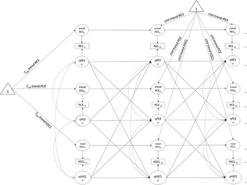
Figure 1 shows a graphical structural equation modeling (SEM) representation of the model with three manifest indicators (RES, PCE, HSCL) measuring within effects of three latent processes (η_RES, η_PCE, η_HSCL) with auto- (η_RES-η_RES, η_PCE-η_PCE, η_HSCL-η_HSCL) and cross-lagged effects (η_RES-η_PCE, η_RES-η_HSCL, η_PCE-η_RES, η_PCE-η_HSCL, η_HSCL-η_RES, η_HSCL-η_PCE), and trends after the first time-point conditioned on the time interval. To examine how the estimated processes have changed after a particular time frame, discrete-time parameters (A’) were computed for different time lags (sessions 1 and 3).

To explore causal inference implications and counterfactuals, we computed plots for the expected change of the latent processes. These plots were generated under deterministic and stochastic conditions. For the deterministic condition, we plotted an independent intervention for each latent process addressing what would happen to process y if we directly intervene on process x? These plots show how the latent processes have changed (based on the particular intervention) after a particular timeframe. For the stochastic condition, we plotted a correlated intervention for all processes addressing what would be expected to happen to the system if we observed a change in the latent process y? This allows us to analyze counterfactual changes in all system processes aligned with the empirical observations. For example, if we see a change of 1.00 in one process, we can expect other processes to also experience a change (according to their system-noise correlation), and so plot their predicted effects accordingly. It is expected that the lower the discrepancies between these two sets of plots (deterministic and stochastic conditions), the higher the reliability to claim causal interpretations, as observational conditions more closely match those of an experiment in which interventions are applied to one process only. Afterwards, the effects of moderators on drift and trend parameters were considered. The significant effects (95% credible intervals not including zero) were plotted, showing the relationship of predictors with discrete-time (one session after activation) auto- and cross-lagged effects.

Results

Patients Characteristics

Table 2 provides an overview of the most important patients’ intake characteristics.

Table 2 . Patients’ characteristics.

Characteristics	Total sample (N = 715)
Age (M years (SD))	38.1 (13.2)
Gender female (n (%))	443 (62.0)
German nationality (n (%))	682 (95.4)
Marital status (n married (%))	219 (30.6)
Education (n > 12 years (%))	343 (48.0)
Inability to work (n (%))	133 (18.6)
Intake of medication (n (%))	593 (69.0)
Comorbidity (n (%))
Two diagnoses	274 (38.3)
Three or more diagnoses	206 (28.8)

Patients showed a mean score of 12.95 (SD = 4.79) on the PHQ-9 and 23.55 (SD = 5.35) on the SES at baseline. The mean score for the PHQ-9 at session 10 was 10.80 (SD = 4.61), showing an effect size of the difference intake-session 10th of Cohen’s d = .51 [.43, .58]. On the HSCL-11, the mean score at session one was 2.15 (SD = .56) and at session ten was 1.96 (SD = .58), with an effect size of the difference intake-session 10th of Cohen’s d = .36 [.29, .44]. The HSCL-11 at session 1 and the pre-treatment PHQ-9 scores were significantly correlated with r = .78.

Continuous Time Dynamic Model

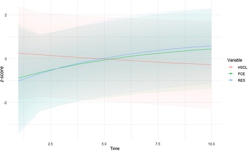
The hierarchical Bayesian CTDM resulted in a log-likelihood of −18,910.5 with 228 parameters and AIC = 38,277. Figure 2 shows the estimated continuous-time trajectories based on the estimated population mean parameters obtained with hierarchical Bayesian CTDM in terms of resource activation (RES), problem-coping experiences (PCE), and symptoms (HSCL). RES and PCE tended to increase, while the HSCL scores tended to decrease over sessions. The color-shaded areas represent the uncertainty of the estimations (95% credible intervals [CI]).

Figure 2 . Estimated trajectories of symptoms, problem-coping experience, and resource activation between sessions one and ten. Note. HSCL = Symptoms; PCE = problem coping experiences; RES = Resource activation.

Auto- and Cross Effects

Table 3 reports the estimates of continuous (i.e., time-independent) and discrete (i.e., time-dependent) time drift parameters. Continuous drift parameters account for direct (causal) effects, describing how processes change from moment to moment. In contrast, discrete-time drift parameters describe how the processes have changed after a specific period, and therefore represent an aggregate of direct and indirect effects over time (Deboeck et al., 2018; Ryan & Hamaker, 2022). The latter are computed from the former by solving the stochastic differential equation for a specific time interval (see Equation 2).

Table 3 . Continuous and discrete time parameter estimates of the hierarchical Bayesian continuous time dynamic model.

Parameters	Continuous time drift (A)	Discrete time drift (A’)
		One session (week) after activation	Three sessions (weeks) after activation
Auto-effects
ηHSCL-ηHSCL	−1.82 [−2.13, −1.53]*	.16 [.12, .20]*	.004 [.002, .008]*
ηRES-ηRES	−3.73 [−4.22, −3.27]*	.02 [.01, .04]*	< .001
ηPCE-ηPCE	−12.41 [−15.69, −9.31]*	.001 [−.002, .005]	< .001
Cross-(lagged) effects
ηRES-ηHSCL	−.52, [−.88, −.14]*	−.04 [−.06, −.01]*	−.001 [−.002, < −.001]*
ηPCE-ηHSCL	.30 [−.78, 1.55]	−.008 [−.02, .01]	< −.001
ηHSCL-ηRES	.51 [.03, .95]*	−.02 [−.05, .01]	< −.001
ηPCE-ηRES	3.57 [2.35, 4.86]*	.01 [.004, .02]*	.00
ηHSCL-ηPCE	−2.28 [−3.08, −1.46]*	−.03 [−.05, −.02]*	< −.001*
ηRES-ηPCE	−.36 [−1.84, 1.09]	.01 [< .001, .02]*	< .001*

Note. HSCL = Symptoms; PCE = Problem coping experiences; RES = Resource activation. In brackets: 95% CI (credible intervals); * significant effects at α = .05 not including zero in the 95% CI

All continuous-time drift parameters were significant, except for the effect of problem coping experience on symptoms (η_PCE-η_HSCL) and resource activation on problem coping experiences (η_RES-η_PCE). These latter non-significant effects indicated that problem-coping experiences have no effect on symptoms, and resource activation has no effect on problem-coping experiences. However, when this latter parameter was transformed to estimate discrete-time cross-lagged effects, resource activation had a significant effect on problem-coping (η_RES-η_PCE). This shows that when resource activation increases by one standardized unit, problem-coping experiences also increase according to the estimated effect after one session. However, this latter effect is small. This difference between the effect observed on continuous- and discrete time parameters can be explained by the presence of indirect effects between the variables of the system and/or the presence of loop/feedback effects between them (e.g., problem-coping experiences have an effect on resource activation, which in turn has an effect on symptoms).

All continuous-time auto effects were negative, which is typical of processes that are self-regulating – the processes tend towards the estimated baseline after unexpected shifts up or down. The change rate of problem-coping experiences (η_PCE-η_PCE) was more negative than the change rate of symptoms (η_HSCL-η_HSCL) and resource activation (η_RES-η_RES), indicating that unexpected changes in problem-coping experiences (η_PCE-η_PCE) tended to dissipate faster than for the other two processes. This shows up in discrete-time as positive auto-regression effects, implying that the constructs tended to predict themselves in the next session, and this predictive power (as expected) declines over time.

Likewise, continuous-time cross-effects showed that resource activation had a negative effect on symptoms (η_RES-η_HSCL). When this parameter was transformed into discrete-time cross-lagged effects, they continued to be negative, implying that when the patient in one session experiences resource activation, a reduction of symptoms tends to occur in the next session. All the effects described tended to dissipate after three sessions.

Exploring Causality and Counterfactuals

To examine causal inference implications and counterfactuals, we plotted the effects based on a manipulated intervention or shock to each latent process under two conditions: deterministic and stochastic (Figure 3). On the top row of Figure 3, a hypothetical intervention of magnitude 1.00 is given to each latent process considering only the deterministic components of the system (independent intervention). In each column, a different latent process receives the intervention. On the lower row, when there is an intervention of 1.00 to a latent process, the other latent processes receive an intervention in accordance with the estimated system noise correlation.

Figure 3 . Hypothetical independent and correlated interventions (shocks) to the latent processes (η) of the hierarchical Bayesian continuous time dynamic model. Note. HSCL = Symptoms; PCE = Problem coping experiences; RES = Resource activation. Color-shaded areas: Uncertainty, 95% CI (credible intervals).

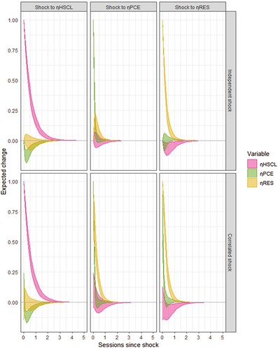
In Figure 3, when analyzing deterministic components only (top left plot), when symptoms (HSCL) receive the intervention (hypothetical manipulation that produces an increment of symptoms), problem-coping experiences (PCE) immediately drops. This implies that when patients increase their symptoms (HSCL), problem-coping experiences (PCE) in the system tends to decline. Furthermore, the expected change of resource activation (RES) shows an area of uncertainty above and below zero at the same time; therefore, the expected change of resource activation (RES) after an intervention on symptoms (HSCL) is not significant. These effects are similar under the observed system conditions (lower left plot of Figure 3), with problem-coping experiences (PCE) having a greater area of uncertainty (above and below zero) immediately after the intervention on symptoms, but completely negative from 0.5 sessions after the intervention. All these effects dissipate between three or four sessions after the intervention.

When problem-coping experiences (PCE) receive the intervention, under deterministic and observed conditions (middle of Figure 3), resource activation (RES) likely follows. That is, if we intervene on the system raising problem-coping experiences by 1.00, resource activation (RES) tends to raise proportionally, showing a greater increment under the observed conditions than the deterministic ones. Thus, other non-controlled processes may be behind the relationship between resource activation (RES) and symptoms (HSCL), making this increment larger when system noise is considered. Nevertheless, the expected change of symptoms (HSCL) shows an area of uncertainty above and below zero at similar time lags under both system conditions; therefore, the expected change of symptoms (HSCL) after an intervention on problem coping experiences (PCE) is not significant.

Finally, when resource activation (RES) receives the intervention under deterministic conditions (top right plot of Figure 3), the expected change of problem-coping experiences (PCE) shows an area of uncertainty above and below zero. However, the expected change of PCE under the stochastic conditions (right lower plot of Figure 3) follows the intervention of resource activation (RES). Thus, other non-measured processes may be influencing this association. After an intervention on resource activation (RES), symptoms (HSCL) tend to drop under both conditions, showing a greater area of uncertainty (above and below zero) under the stochastic system conditions until 0.5 sessions after the intervention, being negative thereafter until three or four sessions.

Effect of Moderators

The effects of moderators on trends were not significant. However, these effects were significant for PHQ-9 on the cross effect of problem-coping experiences on symptoms (PHQ-9: η_PCE-η_HSCL= -.56 [−1.01, -.11], z = −2.56) and the cross effects of symptoms on resource activation (PHQ-9: η_HSCL-η_RES= .34 [.002, .69], z = 2.01). Self-efficacy (SE) had a significant effect on the auto effect of symptoms (SE: η_HSCL-η_HSCL= .14 [.03, .26], z = 2.36), and problem-coping experiences (SE: η_PCE-η_PCE= 1.29 [.35, 2.20], z = 2.75). Additionally, self-efficacy had a significant effect on the cross effects of resource activation on symptoms (SE: η_RES-η_HSCL= -.34 [-.60, -.10], z = −2.66), problem-coping experiences on symptoms (SE: η_PCE-η_HSCL= .52 [.11, .92], z = 2.54), and symptoms on resource activation (SE: η_HSCL-η_RES= .36 [.10, .63], z = 2.67). Figure 4 shows the direction of these effects transformed into discrete-time parameters for Δt = 1 (one session after activation).

Figure 4 . Significant effects of patients’ intake characteristics on discrete time (one session after activation) drift parameters of the hierarchical Bayesian continuous time dynamic model. Note. A) Effect of depression (PHQ-9) on the cross-lagged effects of problem coping experience on symptoms (η_PCE-η_HSCL) and symptoms on resource activation (η_HSCL-η_RES). B) Effect of self-efficacy (SE) on discrete time auto effect of symptoms (η_HSCL-η_HSCL) and problem coping experiences (η_PCE-η_PCE); and cross-lagged effects of resource activation on symptoms (η_RES-η_HSCL), problem coping experiences on symptoms (η_PCE-η_HSCL), and symptoms on resource activation (η_HSCL-η_RES). Color-shaded areas: Uncertainty, 95% CI (credible intervals).

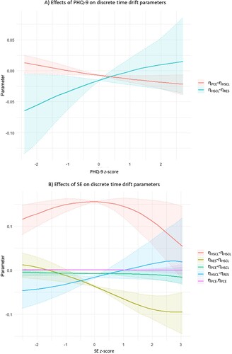
Figure 4A shows the higher the PHQ-9 at intake, the lower the cross-lagged effect of problem-coping experiences on symptoms (η_PCE-η_HSCL). Patients with higher depression levels have a greater tendency to obtain a significant negative effect of problem-coping experiences on symptoms. Thus, for these patients, when they experience more problem coping in one session, the probability of reducing symptoms the following one increases (compared to patients with lower depression levels for whom the trend of the effect is the opposite and the area of uncertainty passes by zero).

Furthermore, the lower the PHQ-9 at intake, the lower the effect of symptoms on resource activation (η_HSCL-η_RES). Patients with lower depression levels have a greater tendency to obtain a negative effect of symptoms on resource activation. Thus, for these patients, when they experience an increase in psychological distress, they tend to hinder the experience of resource activation in the next session. The opposite trend is observed for patients with higher depression scores at intake. However, the area of uncertainty of this latter trend passes by zero, becoming not significant.

Figure 4B shows that for patients with low and high self-efficacy scores at baseline, the auto-effect of symptoms (η_HSCL-η_HSCL) tends to decrease, with patients with higher self-efficacy manifesting a lower effect. Additionally, patients with higher self-efficacy tend to have a lower effect of resource activation on symptoms (η_RES-η_HSCL) compared to patients with lower self-efficacy that obtain the opposite trend. Thus, when self-efficacious patients experience more resource activation in one session, the probability of improving symptoms in the next is higher than for patients with lower self-efficacy. The effect of problem-coping experiences on symptoms (η_PCE-η_HSCL) tends to be higher for patients with lower self-efficacy. However, this effect is small and with uncertainty areas close to zero. For patients with low self-efficacy, the effect of symptoms on resource activation (η_HSCL-η_RES) tends to be negatively lower, implying that when they experience an increase in symptoms, their experience of resource activation results hinders the following session. Finally, self-efficacy has minimal moderating effects on the auto effect of problem experiences (ηPCE-ηPCE).

Discussion

The current study provided an empirical example of integrating two lines of psychotherapy research to improve psychological treatments for depression: the study of moderators (i.e., what works for whom?) and the study of mediators (i.e., how does it work?). In this regard, we extended previous work on psychotherapy research about mediation and change processes (e.g., Hollon & DeRubeis, 2009; Kraemer et al., 2002) going in the direction of analyzing moderated mediations (Hollon, 2019).

Models that can deal with causal inference need to be used to integrate process-outcome and treatment personalization research. To this end, hierarchical Bayesian CTDM was implemented. Nevertheless, as discussed in the introduction, while CTDM can provide insights into causality, in particular the relation between direct effects (i.e., mechanism) and longer-term outcomes, conclusions need to be suitably tempered by the extent of belief in the specified model, and possibilities for confounding should always be considered. In the following, we discuss our main findings, their clinical implications, and how they should be read in the context of multiple sources contributing to the study of causal relationships between the observed phenomena.

Main Findings and Clinical Implications

When only the deterministic components of the system were analyzed (Figure 3, top row), resource activation (as experienced by patients) led to symptom improvement during the first ten sessions of therapy. This effect is short-lasting (i.e., 1–2 sessions). Changes in problem-coping experiences do not seem to have a direct effect on symptoms. Nevertheless, both processes generate a synergy over time in which problem-coping experiences tend to prompt resource activation, in turn generating improvement in symptoms. However, resource activation does not seem to have an effect on problem-coping experiences. This implies that, for patients with depression, a treatment strategy based on both processes will have an effect on symptom improvement. That is a direct effect of resource activation on symptoms, and an indirect effect of problem-coping experiences on symptoms via resource activation.

Simple models of complex processes should not be trusted too far, however– the above description of dynamics is implied by the fitted model, but observational conditions are generally very far from typical experimental scenarios in which one thing can be manipulated at a time. Considering correlated random changes in the system (Figure 3, lower row) can let us see the expected dynamics under the conditions we directly observed, wherein processes are subject to common sources of change. In this case, we observe that the effects of problem-coping experiences on resource activation and vice-versa are considerably larger than under deterministic conditions. This implies that there is a strong correlation between problem-coping experiences and resource activation, suggesting a positive influence of one on the other. However, it is important to consider the possibility of an external variable influencing both processes. When there is a high correlation in system noise, a positive continuous-time cross effect may indicate a slower return to baseline rather than a distinct deviation from baseline, which is typically more noteworthy. While this positive system noise correlation complicates the interpretation of the relationship between problem-coping experiences and resource activation, the absence of a significant system noise correlation between problem-coping experiences and resource activation, and symptoms, provides some reassurance that changes in problem-coping experiences and resource activation may indeed be driving changes in symptoms.

A non-measured variable that might influence the relationship between problem-coping experiences and resource activation may be therapeutic relationship and alliance. For instance, therapeutic relationship and alliance probably interacted with these effects (Moggia et al., 2022), making that, under the conditions of a good therapeutic relationship and alliance, when patients experienced a rise in one of them, the other was likely to follow.

Other factors that may contribute to random changes and variability are that the evaluated processes were measured with self-reports from the patients’ perspective. They do not represent formalized or systematic interventions implemented by the therapist. So, the patient could have had the experience of problem coping and/or resource activation in a particular session when the therapist was not explicitly working on that aim. In this sense, the in-session experiences of problem-coping and resource activation were probably influenced by the patient’s perceptions and attitudes towards therapy and the therapist (Rubel et al., 2017). Furthermore, after the session, patients probably tried to implement the experience of problem-coping and/or resource activation in their everyday life. Thus, outside therapy, these processes probably interacted with multiple other psychological and social variables and life circumstances at different levels, which in turn affected treatment outcome.

Furthermore, the therapeutic arsenal with which therapists count under an integrative CBT framework is much broader than problem coping and resource activation. Many other interventions and processes that were not analyzed may play a role in the system, influencing the effect of problem-coping experiences and resource activation on symptoms, and the patient’s perception of them.

When analyzing the role of moderators and individual differences, patients with higher depression levels tended to have a negative and lower effect of problem-coping experiences on symptoms, and symptoms on resource activation. That is, more severe patients had a tendency to improve symptoms after an increase in problem-coping experiences and tended to reduce their experience of resource activation when they worsened.

Patients with lower self-efficacy tended to have a negative but higher effect of resource activation on symptoms, and a positive effect in the opposite direction (symptoms on resource activation). Thus, patients with low self-efficacy tended to present a smaller improvement of symptoms when they experienced resource activation (compared to patients with high self-efficacy), and their experience of resource activation was hindered when they deteriorated.

High self-efficacious patients presented a lower auto effect of psychological distress than patients with low self-efficacy. That is, when high self-efficacious patients experienced distress, this experience dissipated faster than for patients with low self-efficacy. Additionally, highly self-efficacious patients had a negative and lower effect of resource activation on symptoms. Thus, patients with high self-efficacy improved more after experiencing resource activation than patients with low self-efficacy.

In terms of clinical recommendations, the previous findings imply that for patients with high depression and low self-efficacy, a treatment strategy based on promoting problem-coping experiences can be recommended, especially at the beginning of therapy. These patients have a tendency to improve after experiencing problem coping. At the same time, problem-coping experiences foster the experience of resource activation, which in turn has a significant effect on symptoms. In contrast, for patients with mild-moderate depression and high self-efficacy, a treatment strategy based on emphasizing resource activation can be recommended.

When interpreting the previous effects, it should be taken into account that the symptom measure (HSCL-11), just like the depression measure (PHQ-9), also assesses depression items, which means that these two instruments are associated with each other and cover partly overlapping constructs. This is generally the case for most symptom-based outcome measures, which are often moderately to strongly correlated with each other. Moreover, the PHQ-9 was used as a time-independent predictor, while the HSCL-11 was used as a time-dependent measure with its own trend to track change in outcome. In this sense, there are no confoundings between both measures.

Causal Inference Implications

Our results should be read under a pluralistic framework of causal inference (Oddli et al., 2022), considering our findings as preliminary insights in that direction. Under deterministic conditions, resource activation has an effect on symptom improvement, and when system noise is considered, this effect continues manifesting. However, when resource activation increases, the immediate effect on symptoms (reducing psychological distress) shows higher uncertainty. This implies that this effect may be affected by a common non-measured variable (as we mentioned before). Aligned with our findings, there is experimental evidence on the effect of using specific resource activation techniques (e.g., solution-focused questions) on reducing immediate negative affect (Braunstein & Grant, 2016; Grant, 2012; Grant & Gerrard, 2020; Neipp et al., 2016). Similarly, a recent meta-analysis about process-outcome studies on strength-based methods (i.e., resource activation; Flückiger et al., 2023), found that these interventions were linked with more favorable immediate, session-level outcomes. The authors concluded that these effects might not be a trivial by-product of treatment progress and may provide a unique contribution to psychotherapy outcomes.

The effect of problem-coping experiences on symptoms was not significant under the two analyzed system conditions. However, the moderation of depression levels on this effect and the indirect effect of problem-coping experiences on symptoms through resource activation should be clinically considered. Here patients with higher depression levels can present a significant effect of problem-coping experience on symptoms, contributing to the synergy generated by both processes on patient improvement.

From a theoretical perspective, both processes have been pointed out as transtheoretical and as general change mechanisms present in every psychotherapy approach (Grawe, 1997). In this context, there are studies providing evidence of their role in outcome during diverse psychological treatments (e.g., Flückiger et al., 2009; Gassmann & Grawe, 2006; Gmeinwieser et al., 2019, 2020). This transtheoretical conceptualization (and supporting evidence) aligns with our findings. It points out the effect of both processes on outcome improvement. At the same time, it supports that beyond them are other processes that may be playing a role in causing improvement and that both processes may be consequences of other treatment strategies. That is, a specific intervention may produce the experience of problem-coping and resource activation when it is not aimed at that end. On the other way around, interventions aimed at promoting problem-coping experiences and resource activation may produce effects on other uncontrolled processes.

All in all, problem-coping experiences and resource activation can be considered important processes that play a role in symptom improvement in the context of integrative CBT for depression. Nevertheless, both processes are highly correlated and they may be part of the same underlying construct or might be affected by the same external variables.

Strengths, Limitations and Future Directions

Our study was observational and naturalistic, no manipulation of variables was conducted. In this sense, we choose a method to study hypothetical causality under these conditions. We accounted for stable and slow confounders with random effects parameters and covariates, and fast confounders with the correlated system noise. However, confounders which vary at a similar rate to the analysed processes are not easy to account for, and it should be considered carefully to what extent they might exist (Clare et al., 2019; Streeter et al., 2017). Controlling all variables involved in psychotherapy and human change processes is impossible in this sense. While it is true that there were small differences between the deterministic and stochastic conditions under which the effects of the processes were tested, no direct, straightforward causal relationships can be established. In this sense, future studies should replicate (or not) our findings and discuss them in the context of evidence from diverse other studies (using diverse methods) and sources (Krieger & Davey Smith, 2016; Oddli et al., 2022; Rohrer & Murayama, 2021).

One advantage of CTDM over other methods is that it assumes time as a continuous variable. This allows the disentanglement of direct and indirect cross-effects between variables, making it a robust method to study potential causal implications. In psychotherapy research, when considering time as continuous, estimating the effect of the processes between sessions is possible. Even though this is not an empirical evaluation of the implementation of these processes by the patient outside therapy, it is an approximation, assuming that the processes therapists and patients activate in the session can have continued effects afterwards. In this sense, studies incorporating ecological momentary assessment (EMA) to track the implementation of these processes (and others) and their effects on patients’ everyday lives constitute an important contribution to the field (Hehlmann et al., 2021). This potential should be made use of and integrated into studies like the current one using a modeling approach such as CTDM.

CTDM constitutes a flexible approach in terms of the different models that can be estimated (with different parameters and diverse relationships between them), sample size and measurement occasions. However, there is no consensus on how to estimate requirements for statistical power, sample size and frequency of measurements. There is some evidence suggesting that the more auto-stable the processes are, the larger the sample size required. Similarly, a high frequency of measurement occasions is required to detect large effect sizes on the drift parameters (low autostability; Adolf et al., 2021). A simulation study on univariate models suggested that shorter time series can be compensated with larger samples and vice-versa (Hecht & Zitzmann, 2021). The authors estimated the required sample sizes and measurement occasions to fill different model requirements. However, further research is necessary to provide similar estimations with different numbers of variables (beyond univariate models) and combinations of parameters.

Regarding treatment personalization research, it advocates for the implementation of a data-driven approach to personalization (Cohen et al., 2021). This approach analyzes numerous variables (moderators, predictors) from large datasets of previously treated patients to develop algorithms for clinical recommendations (Lutz, Schwartz, et al., 2022). In the current study, we tested only two moderators because including a multitude of predictors in CTDM can be complex and computationally demanding. Therefore, the inclusion of multiple moderators to address patient heterogeneity can be done with post-hoc estimations based on methods which use the individual-level parameters of the fitted model. For instance, from a dataset of previously treated patients, diverse CTDM can be estimated following a classification of patient profiles identified by cluster analysis. Neuronal networks can be used to predict the continuous time drift parameters (multiple outcome variables) using numerous predictors. In that way, the dynamics of the system and the specific discrete time effects for the new patient can be estimated.

Another approach to treatment personalization comes from the utilization of the nearest neighbors algorithm. There, a new patient is matched with a group of previously treated similar patients from an archived dataset. This matching procedure is based on patient pre-treatment characteristics. A CTDM can then be computed based on the group of patients with the characteristics most similar to the new patient. The nearest neighbors algorithm (although not CTDM) is the approach implemented by Lutz et al. (2019) in the Trier Treatment Navigator (TTN; a clinical decision support system) to make pre-treatment strategy recommendations and estimate the expected treatment response to evaluate the patient progress during treatment. In this regard, models based on CTDM might be implemented into clinical decision support systems like the TTN.

The complexities of CTDM allow for the analysis of a limited number of processes. Therefore, the researcher applying this approach should carefully decide which processes to include in the model. In addition, the clinical setting from which the data is collected should have implemented not only routine outcome monitoring (Lutz, Rubel, et al., 2022) but routine process monitoring as well. This is necessary to ensure valid and reliable psychotherapy process measures are included in the analyses. In our study, we used a patient self-report measure. This represents a limitation because the processes or strategies implemented by the therapist in a specific session may not match the patient’s perspective and vice-versa (as we already explained). The most valid and reliable measures in this regard might be those reported by independent raters (e.g., Inventory of Therapeutic Interventions and Skills [ITIS]; Boyle et al., 2020).

Nevertheless, the routine implementation of independent ratings in naturalistic settings is impractical. It requires the examination of video or audio recordings of sessions (which is a time and resource-intensive task) by raters trained in the application of the measure. Therefore, the incorporation of routine process monitoring should rely on validated patient and therapist self-report measures. However, some progress has been made in the implementation of natural language processing (NLP) algorithms to automatically detect therapeutic strategies, interventions, and processes applied in sessions (e.g., Goldberg et al., 2021). Future clinical decision support systems should work to incorporate these technologies to increase the precision and specificity of their personalized recommendations.

Conclusion

Resource activation was strongly associated with symptom improvement in psychotherapy for depression. Problem-coping experiences tend to promote resource activation. A treatment strategy based on promoting problem-coping experiences can be recommended for patients with severe depression and low self-efficacy. For patients with mild-moderate depression and high self-efficacy, a treatment strategy based on promoting resource activation can be recommended. Considering that problem-coping experiences and resource activation were highly correlated, further research is required to clarify the causal dynamics between them and outcome, and to personalize treatments based on them.

Disclosure Statement

No potential conflict of interest was reported by the author(s).

Notes

1 We followed the definition of therapeutic processes stated by Hofmann and Hayes (2019): “Therapeutic processes are the underlying change mechanisms that lead to the attainment of a desirable treatment goal. We define a therapeutic process as a set of theory-based, dynamic, progressive, and multilevel changes that occur in predictable empirically established sequences oriented toward the desirable outcomes. These processes are theory-based and associated with falsifiable and testable predictions, they are dynamic because processes may involve feedback loops and nonlinear changes, they are progressive in the long term in order to be able to reach the treatment goal, and they form a multilevel system because some processes supersede others. Finally, these processes are oriented toward both immediate and long-term goals.” (p. 38) [Italics in the original].

2 In calculus, the derivative of a function represents the instantaneous rate of change of the function value (dependent variable) concerning a change in its argument (independent variables).

3 A stochastic process is a mathematical function that relates random variables accounting for the occurrence of random events or the succession of random steps in a given mathematical space (i.e., random walk).

4 W(t) corresponds to a Wiener stochastic process (also called Brownian motion) characterized by independent and normally distributed increments that are continuous in time. The derivate of a Wiener stochastic process is white noise. In discrete-time systems, white noise represents the effect on the system of independent and identically normally distributed random variables (i.e., serially uncorrelated random variables with zero mean and finite variance).

5 This contrasts with discrete-time cross-lagged panels where an earlier state of the system is used to predict the new level of the processes.

6 It should be considered that the stochastic component (or system noise) is not equivalent to the residuals in traditional regression models (as there may be a measurement layer between the latent process and the observations).

References

- Adolf, J. K., Loossens, T., Tuerlinckx, F., & Ceulemans, E. (2021). Optimal sampling rates for reliable continuous-time first-order autoregressive and vector autoregressive modeling. Psychological Methods, 26(6), 701–718. https://doi.org/10.1037/met0000398
- American Psychiatric Association. (2000). Diagnostic and Statistical Manual of Mental Disorders—IV - Text Revised. Author.
- Barkham, M., & Lambert, M. J. (2021). The efficacy and effectiveness of psychological therapies. In M. Barkham, W. Lutz, & L. G. Castonguay (Eds.), Bergin and Garfield’s handbook of psychotherapy and behavior change: 50th anniversary edition (pp. 135–189). John Wiley & Sons, Inc.
- Bavojdan, M. R., Towhidi, A., & Rahmati, A. (2011). The Relationship between Mental Health and General Self-Efficacy Beliefs, Coping Strategies and Locus of Control in Male Drug Abusers. Addiction and Health, 3(3–4), 111–118.
- Boyle, K., Deisenhofer, A.-K., Rubel, J. A., Bennemann, B., Weinmann-Lutz, B., & Lutz, W. (2020). Assessing treatment integrity in personalized CBT: The inventory of therapeutic interventions and skills. Cognitive Behaviour Therapy, 49(3), 210–227. https://doi.org/10.1080/16506073.2019.1625945
- Braunstein, K., & Grant, A. M. (2016). Approaching solutions or avoiding problems? The differential effects of approach and avoidance goals with solution-focused and problem-focused coaching questions. Coaching: An International Journal of Theory, Research and Practice, 9(2), 93–109. https://doi.org/10.1080/17521882.2016.1186705
- Bronisch, T., Hiller, W., Mombour, W., & Zaudig, M. (1996). International diagnostic checklists for personality disorders according to ICD-10 and DSM-IV—IDCL-P. Hogrefe & Huber Publishers.
- Cheavens, J. S., Strunk, D. R., Lazarus, S. A., & Goldstein, L. A. (2012). The compensation and capitalization models: A test of two approaches to individualizing the treatment of depression. Behaviour Research and Therapy, 50(11), 699–706. https://doi.org/10.1016/j.brat.2012.08.002
- Clare, P. J., Dobbins, T. A., & Mattick, R. P. (2019). Causal models adjusting for time-varying confounding—A systematic review of the literature. International Journal of Epidemiology, 48(1), 254–265. https://doi.org/10.1093/ije/dyy218
- Cohen, Z. D., Delgadillo, J., & DeRubeis, R. (2021). Personalized treatment approaches. In M. Barkham, W. Lutz, & L. G. Castonguay (Eds.), Bergin and garfield’s handbook of psychotherapy and behavior change (50th Anniversary Edition, pp. 673–704). Wiley.
- Coyne, J. C., Kessler, R. C., Tal, M., Turnbull, J., Wortman, C. B., & Greden, J. F. (1987). Living with a depressed person. Journal of Consulting and Clinical Psychology, 55(3), 347–352. https://doi.org/10.1037/0022-006X.55.3.347
- Crits-Christoph, P., Gibbons, C., & B, M. (2021). Psychotherapy process-outcome research: Advances in understanding causal connections. In M. Barkham, W. Lutz, & L. G. Castonguay (Eds.), Bergin and garfield’s handbook of psychotherapy and behavior change ((7th ed, pp. 263–296). Wiley.
- Cuijpers, P., Quero, S., Noma, H., Ciharova, M., Miguel, C., Karyotaki, E., Cipriani, A., Cristea, I. A., & Furukawa, T. A. (2021). Psychotherapies for depression: A network meta-analysis covering efficacy, acceptability and long-term outcomes of all main treatment types. World Psychiatry, 20(2), 283–293. https://doi.org/10.1002/wps.20860
- Cuijpers, P., Reijnders, M., Karyotaki, E., de Wit, L., & Ebert, D. D. (2018). Negative effects of psychotherapies for adult depression: A meta-analysis of deterioration rates. Journal of Affective Disorders, 239, 138–145. https://doi.org/10.1016/j.jad.2018.05.050
- Deboeck, P. R., & Preacher, K. J. (2016). No need to be discrete: A method for continuous time mediation analysis. Structural Equation Modeling: A Multidisciplinary Journal, 23(1), 61–75. https://doi.org/10.1080/10705511.2014.973960
- Deboeck, P. R., Preacher, K. J., & Cole, D. A. (2018). Mediation modeling: Differing perspectives on time alter mediation inferences. In K. van Montfort, J. H. L. Oud, & M. C. Voelkle (Eds.), Continuous Time Modeling in the Behavioral and Related Sciences (pp. 179–203). Springer International Publishing. https://doi.org/10.1007/978-3-319-77219-6_8
- Derogatis, L. R. (1994). SCL-90-R : Symptom checklist-90-R : administration, scoring & procedures manual. National Computer Systems, Inc.
- Doss, B. D. (2004). Changing the way we study change in psychotherapy. Clinical Psychology: Science and Practice, 11(4), 368–386. https://doi.org/10.1093/clipsy.bph094
- Driver, C. C. (2017). Hierarchical continuous time dynamic modelling for psychology and the social sciences. Humboldt-Universität zu Berlin. https://edoc.hu-berlin.de/bitstream/handle/18452/19659/dissertation_driver_charles.pdf?sequence=3.
- Driver, C. C. (2022). Inference with cross-lagged effects—Problems in time [Preprint]. Open Science Framework. https://doi.org/10.31219/osf.io/xdf72
- Driver, C. C., & Tomasik, M. J. (2022). Inference with cross-lagged effects—common causes in dynamic systems [Preprint]. Open Science Framework. https://doi.org/10.31219/osf.io/xdf72
- Driver, C. C., & Voelkle, M. C. (2018). Hierarchical Bayesian continuous time dynamic modeling. Psychological Methods, 23(4), 774–799. https://doi.org/10.1037/met0000168
- Driver, C. C., Voelkle, M. C., & Oud, H. (2022). ctsem: Continuous time structural equation modelling version 3.6.0. https://cran.r-project.org/web/packages/ctsem/ctsem.pdf.
- Flückiger, C., Caspar, F., Holtforth, M. G., & Willutzki, U. (2009). Working with patients’ strengths: A microprocess approach. Psychotherapy Research, 19(2), 213–223. https://doi.org/10.1080/10503300902755300
- Flückiger, C., Munder, T., Del Re, A. C., & Solomonov, N. (2023). Strength-based methods – a narrative review and comparative multilevel meta-analysis of positive interventions in clinical settings. Psychotherapy Research, 1–17. https://doi.org/10.1080/10503307.2023.2181718
- Flückiger, C., Regli, D., Zwahlen, D., Hostettler, S., & Caspar, F. (2010). Der Berner Patienten- und Therapeutenstundenbogen 2000. Zeitschrift für Klinische Psychologie und Psychotherapie, 39(2), 71–79. https://doi.org/10.1026/1616-3443/a000015
- Gassmann, D., & Grawe, K. (2006). General change mechanisms: The relation between problem activation and resource activation in successful and unsuccessful therapeutic interactions. Clinical Psychology & Psychotherapy, 13(1), 1–11. https://doi.org/10.1002/cpp.442
- Gmeinwieser, S., Hagmayer, Y., Pieh, C., & Probst, T. (2019). General change mechanisms in the early treatment phase and their associations with the outcome of cognitive behavioural therapy in patients with different levels of motivational incongruence. Clinical Psychology & Psychotherapy, 26(5), 550–561. https://doi.org/10.1002/cpp.2381
- Gmeinwieser, S., Kuhlencord, M., Ruhl, U., Hagmayer, Y., & Probst, T. (2020). Early developments in general change mechanisms predict reliable improvement in addition to early symptom trajectories in cognitive behavioral therapy. Psychotherapy Research, 30(4), 462–473. https://doi.org/10.1080/10503307.2019.1609709
- Goldberg, S. B., Tanana, M., Imel, Z. E., Atkins, D. C., Hill, C. E., & Anderson, T. (2021). Can a computer detect interpersonal skills? Using machine learning to scale up the Facilitative Interpersonal Skills task. Psychotherapy Research, 31(3), 281–288. https://doi.org/10.1080/10503307.2020.1741047
- Gómez Penedo, J. M., Schwartz, B., Giesemann, J., Rubel, J. A., Deisenhofer, A.-K., & Lutz, W. (2022). For whom should psychotherapy focus on problem coping? A machine learning algorithm for treatment personalization. Psychotherapy Research, 32(2), 151–164. https://doi.org/10.1080/10503307.2021.1930242
- Grant, A. M. (2012). Making positive change: A randomized study comparing solution-focused vs. Problem-focused coaching questions. Journal of Systemic Therapies, 31(2), 21–35. https://doi.org/10.1521/jsyt.2012.31.2.21
- Grant, A. M., & Gerrard, B. (2020). Comparing problem-focused, solution-focused and combined problem-focused/solution-focused coaching approach: Solution-focused coaching questions mitigate the negative impact of dysfunctional attitudes. Coaching: An International Journal of Theory, Research and Practice, 13(1), 61–77. https://doi.org/10.1080/17521882.2019.1599030
- Grawe, K. (1997). Research-informed psychotherapy. Psychotherapy Research, 7(1), 1–19. https://doi.org/10.1080/10503309712331331843
- Grosz, M. P., Rohrer, J. M., & Thoemmes, F. (2020). The taboo against explicit causal inference in nonexperimental psychology. Perspectives on Psychological Science, 15(5), 1243–1255. https://doi.org/10.1177/1745691620921521
- Hansen, N., & Sokol, A. (2014). Causal interpretation of stochastic differential equations. Electronic Journal of Probability, 19. https://doi.org/10.1214/EJP.v19-2891
- Hecht, M., & Zitzmann, S. (2021). Sample size recommendations for continuous-time models: Compensating shorter time series with larger numbers of persons and vice versa. Structural Equation Modeling: A Multidisciplinary Journal, 28(2), 229–236. https://doi.org/10.1080/10705511.2020.1779069
- Hehlmann, M. I., Schwartz, B., Lutz, T., Gómez Penedo, J. M., Rubel, J. A., & Lutz, W. (2021). The use of digitally assessed stress levels to model change processes in CBT - A feasibility study on seven case examples. Frontiers in Psychiatry, 12, 613085. https://doi.org/10.3389/fpsyt.2021.613085
- Hofmann, S. G., & Hayes, S. C. (2019). The future of intervention science: Process-based therapy. Clinical Psychological Science, 7(1), 37–50. https://doi.org/10.1177/2167702618772296
- Hollon, S. D. (2019). Moderation, mediation, and moderated mediation. World Psychiatry, 18(3), 288–289. https://doi.org/10.1002/wps.20665
- Hollon, S. D., & DeRubeis, R. J. (2009). Mediating the effects of cognitive therapy for depression. Cognitive Behaviour Therapy, 38(sup1), 43–47. https://doi.org/10.1080/16506070902915667
- Huibers, M. J. H., Lorenzo-Luaces, L., Cuijpers, P., & Kazantzis, N. (2021). On the road to personalized psychotherapy: A research agenda based on cognitive behavior therapy for depression. Frontiers in Psychiatry, 11, 607508. https://doi.org/10.3389/fpsyt.2020.607508
- Kraemer, H. C., Wilson, G. T., Fairburn, C. G., & Agras, W. S. (2002). Mediators and moderators of treatment effects in randomized clinical trials. Archives of General Psychiatry, 59(10), 877. https://doi.org/10.1001/archpsyc.59.10.877
- Krieger, N., & Davey Smith, G. (2016). The tale wagged by the DAG: Broadening the scope of causal inference and explanation for epidemiology. International Journal of Epidemiology, dyw114. https://doi.org/10.1093/ije/dyw114
- Kroenke, K., Spitzer, R. L., & Williams, J. B. W. (2001). The PHQ-9: Validity of a brief depression severity measure. Journal of General Internal Medicine, 16(9), 606–613. https://doi.org/10.1046/j.1525-1497.2001.016009606.x
- Lambert, M. J. (2005). Early response in psychotherapy: Further evidence for the importance of common factors rather than “placebo effects”. Journal of Clinical Psychology, 61(7), 855–869. https://doi.org/10.1002/jclp.20130
- Larson, R., & Edwards, B. (2022). Calculus (12th ed.). Cengage.
- Lok, J. J. (2008). Statistical modeling of causal effects in continuous time. The Annals of Statistics, 36(3). https://doi.org/10.1214/009053607000000820
- Luszczynska, A., Gutiérrez-Doña, B., & Schwarzer, R. (2005). General self-efficacy in various domains of human functioning: Evidence from five countries. International Journal of Psychology, 40(2), 80–89. https://doi.org/10.1080/00207590444000041
- Lutz, W., Rubel, J. A., Schwartz, B., Schilling, V., & Deisenhofer, A.-K. (2019). Towards integrating personalized feedback research into clinical practice: Development of the Trier Treatment Navigator (TTN). Behaviour Research and Therapy, 120, 103438. https://doi.org/10.1016/j.brat.2019.103438
- Lutz, W., Rubel, J., Deisenhofer, A., & Moggia, D. (2022). Continuous outcome measurement in modern data-informed psychotherapies. World Psychiatry, 21(2), 215–216. https://doi.org/10.1002/wps.20988
- Lutz, W., Schwartz, B., & Delgadillo, J. (2022). Measurement-based and data-informed psychological therapy. Annual Review of Clinical Psychology, 18(1), 71–98. https://doi.org/10.1146/annurev-clinpsy-071720-014821
- Lutz, W., Schwartz, B., Hofmann, S. G., Fisher, A. J., Husen, K., & Rubel, J. A. (2018). Using network analysis for the prediction of treatment dropout in patients with mood and anxiety disorders: A methodological proof-of-concept study. Scientific Reports, 8(1), 7819. https://doi.org/10.1038/s41598-018-25953-0
- Lutz, W., Tholen, S., Schürch, E., & Berking, M. (2006). Reliabilität von Kurzformen gängiger psychometrischer Instrumente zur Evaluation des therapeutischen Fortschritts in Psychotherapie und Psychiatrie. Diagnostica, 52(1), 11–25. https://doi.org/10.1026/0012-1924.52.1.11
- Moggia, D., Lutz, W., Arndt, A., & Feixas, G. (2020). Patterns of change and their relationship to outcome and follow-up in group and individual psychotherapy for depression. Journal of Consulting and Clinical Psychology, 88(8), 757–773. https://doi.org/10.1037/ccp0000562
- Moggia, D., Schwartz, B., Rubel, J. A., Zimmermann, D., Kästel, B., & Lutz, W. (2022). Is it me, is it you or is it both of US? Applying the social relations model to disentangle the components of the therapeutic bond. Psychotherapy Research, 30–44. https://doi.org/10.1080/10503307.2022.2126334
- Neipp, M.-C., Beyebach, M., Nuñez, R. M., & Martínez-González, M.-C. (2016). The effect of solution-focused versus problem-focused questions: A replication. Journal of Marital and Family Therapy, 42(3), 525–535. https://doi.org/10.1111/jmft.12140
- Oddli, H. W., Stänicke, E., Halvorsen, M. S., & Lindstad, T. G. (2022). Causality in psychotherapy research: Towards evidential pluralism. Psychotherapy Research, 1–15. https://doi.org/10.1080/10503307.2022.2161433
- Oud, J. H. L., & Voelkle, M. C. (2014). Do missing values exist? Incomplete data handling in cross-national longitudinal studies by means of continuous time modeling. Quality & Quantity, 48(6), 3271–3288. https://doi.org/10.1007/s11135-013-9955-9
- Papakostas, G. I., & Fava, M. (2008). Predictors, moderators, and mediators (correlates) of treatment outcome in major depressive disorder. Dialogues in Clinical Neuroscience, 10(4), 439–451. https://doi.org/10.31887/DCNS.2008.10.4/gipapakostas
- Pearl, J., & Mackenzie, D. (2018). The book of why: The new science of cause and effect. Basic Books.
- Rohrer, J. M., & Murayama, K. (2021). These are not the effects you are looking for: Causality and the within-/between-person distinction in longitudinal data analysis [Preprint]. PsyArXiv. https://doi.org/10.31234/osf.io/tg4vj
- Rubel, J. A., Rosenbaum, D., & Lutz, W. (2017). Patients’ in-session experiences and symptom change: Session-to-session effects on a within- and between-patient level. Behaviour Research and Therapy, 90, 58–66. https://doi.org/10.1016/j.brat.2016.12.007
- Rubel, J., Lutz, W., Kopta, S. M., Köck, K., Minami, T., Zimmermann, D., & Saunders, S. M. (2015). Defining early positive response to psychotherapy: An empirical comparison between clinically significant change criteria and growth mixture modeling. Psychological Assessment, 27(2), 478–488. https://doi.org/10.1037/pas0000060
- Ryan, O., & Hamaker, E. L. (2022). Time to intervene: A continuous-time approach to network analysis and centrality. Psychometrika, 87(1), 214–252. https://doi.org/10.1007/s11336-021-09767-0
- Schlagert, H. S., & Hiller, W. (2017). The predictive value of early response in patients with depressive disorders. Psychotherapy Research, 27(4), 488–500. https://doi.org/10.1080/10503307.2015.1119329
- Schwarzer, R., & Jerusalem, M. (1995). Generalized Self-Efficacy scale. In J. Weinman, S. Wright, & M. Johnston (Eds.), Measures in health psychology: A user’s portfolio. Causal and control beliefs (pp. 35–37). NFER-NELSON.
- Simon, G. E., & Ludman, E. J. (2010). Predictors of early dropout from psychotherapy for depression in community practice. Psychiatric Services, 61(7), 684–689. https://doi.org/10.1176/ps.2010.61.7.684
- Streeter, A. J., Lin, N. X., Crathorne, L., Haasova, M., Hyde, C., Melzer, D., & Henley, W. E. (2017). Adjusting for unmeasured confounding in nonrandomized longitudinal studies: A methodological review. Journal of Clinical Epidemiology, 87, 23–34. https://doi.org/10.1016/j.jclinepi.2017.04.022
- Voelkle, M. C., & Oud, J. H. L. (2015). Relating latent change score and continuous time models. Structural Equation Modeling: A Multidisciplinary Journal, 22(3), 366–381. https://doi.org/10.1080/10705511.2014.935918
- Voelkle, M. C., Oud, J. H. L., Davidov, E., & Schmidt, P. (2012). An SEM approach to continuous time modeling of panel data: Relating authoritarianism and anomia. Psychological Methods, 17(2), 176–192. https://doi.org/10.1037/a0027543
- Wampold, B. E., & Imel, Z. E. (2015). The great psychotherapy debate: The evidence for what makes psychotherapy work (Second ed.). Routledge.
- Wittchen, H. U., Wunderlich, U., Gruschwitz, S., & Zaudig, M. (1997). SKID I. Strukturiertes Klinisches Interview für DSM-IV. Achse I: Psychische Störungen. Interviewheft und Beurteilungsheft. Eine deutschsprachige, erweiterte Bearb. D. Amerikanischen Originalversion des SKID I. Hogrefe.
- Zisook, S., Johnson, G. R., Tal, I., Hicks, P., Chen, P., Davis, L., Thase, M., Zhao, Y., Vertrees, J., & Mohamed, S. (2019). General predictors and moderators of depression remission: A VAST-D report. American Journal of Psychiatry, 176(5), 348–357. https://doi.org/10.1176/appi.ajp.2018.18091079
- Zyphur, M. J., Allison, P. D., Tay, L., Voelkle, M. C., Preacher, K. J., Zhang, Z., Hamaker, E. L., Shamsollahi, A., Pierides, D. C., Koval, P., & Diener, E. (2020). From data to causes I: Building a general cross-lagged panel model (GCLM). Organizational Research Methods, 23(4), 651–687. https://doi.org/10.1177/1094428119847278