The Role of Credit Attributes in Explaining the Homeownership Gap Between Whites and Minorities Since the Financial Crisis, 2012–2018

ABSTRACT

Homeownership rates have been slow to recover since the financial crisis. Minority groups such as Blacks and Hispanics have been particularly slow to transition to homeownership. Using uniquely constructed anonymized household panel data obtained from a credit bureau, we find that Blacks and Hispanics were, respectively, one half and two thirds as likely as Whites to transition to mortgage ownership between 2012 and 2018. We analyze the role of credit attributes, among other factors, in explaining the racial/ethnic gap in transition to mortgage ownership by 2018 for a sample of individuals who were nonmortgage holders in 2012. Using the Blinder–Oaxaca decomposition technique for nonlinear equations, we find that racial/ethnic differences in credit attributes explain a large portion of the White–minority gap in the transition rates. However, there are key differences in experience across the two minority groups. Whereas racial/ethnic differences in geographic location contribute substantially to the White–Hispanic gap in the mortgage transition rate, racial/ethnic differences in household composition and income growth matter more in explaining the White–Black gap in the mortgage transition rate. Lastly, we find there is considerable heterogeneity across states in the contribution of credit attributes and geography to the White–minority gap in the transition rate.

KEYWORDS:

• mortgage transition
• Black
• Hispanic
• Blinder–Oaxaca decomposition
• credit attributes

By nearly all measures, the Great Recession of 2008–2009 was the most severe economic contraction in the United States since the Great Depression. The crisis has led to dramatic changes in the U.S. residential mortgage market. The homeownership rate declined substantially, from 67.4% in 2009 to 64.4% in 2018, according to the U.S. Census Bureau’s Housing Vacancy Survey data.¹ The Black and Hispanic homeownership rates also declined during this time.² At the center of the Great Recession was a subprime mortgage crisis that disproportionately affected Black and Hispanic homeowners. New mortgage originations declined whereas foreclosures and other reversals in homeownership increased, wiping out gains in minority homeownership rates. An estimated 8% of Black and 8% of Hispanic homeowners who obtained a mortgage between 2005 and 2008 lost their homes to foreclosure by 2009, compared with 4.5% of non-Hispanic White homeowners (Bocian, Ernst, & Li, 2010).

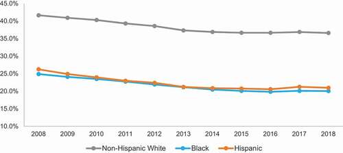
In 2006, 25% of 12.2 million new mortgages³ were to Black or Hispanic borrowers, according to the Home Mortgage Disclosure Act (HMDA) data. By 2009, only 12% of 8.3 million new mortgages were originated to Black or Hispanic borrowers. Figure 1 plots the annual individual-level ownership rate of houses with a mortgage or loan using 1-year American Community Survey public-use microdata (ACS PUMS), for non-Hispanic Whites, Blacks, and Hispanics respectively.⁴ As the figure suggests, Black and Hispanic mortgage ownership rates declined from 25% and 26% in 2008 to 20% and 21% in 2018, respectively. As of 2018, the White–Black and White–Hispanic mortgage ownership gaps stood at roughly 17 percentage points and 16 percentage points, respectively. In this article, we focus on the trends in new mortgages as a key component in understanding the trends in racial differences in mortgage ownership.

Figure 1. Annual mortgage ownership rate at the individual level, 2008–2018

Note. The figure plots the annual homeownership rates on the y-axis for the Non-Hispanic White (gray line), Hispanic (orange line), and Black (blue line) populations. Authors' calculations using American Community Survey public-use microdata, 1-year estimates, United States Census Bureau 2008–2018.

Historically, several government policies have been successful in increasing access to mortgage financing for minority borrowers, such as the government-regulated Government Sponsored Enterprise (GSE) mortgages, the Community Reinvestment Act (CRA) and GSEs’ affordable housing goals (Bostic & Surette, 2001; Gabriel & Rosenthal, 2008),⁵ and low-down payment mortgages backed by Ginnie Mae and GSEs. Despite these initiatives, the racial/ethnic homeownership gap is far from being alleviated, and in fact has been widening for Blacks since the financial crisis. Although there has been a slight uptick in the Hispanic homeownership rate during the recovery period from the Great Recession, the Black homeownership rate was at the same level in 2019 as in 1968 when the Fair Housing Act was adopted. What are some major barriers to mortgage ownership transition following the crisis—changing demographics, credit conditions, or geography? What factors explain the unequal recovery across the two minority groups? This article investigates these key questions using uniquely constructed administrative data.

Our article makes two key contributions. First, we investigate the more recent trends for consumers acquiring new mortgages, including the role of credit attributes likely used by the lenders in originating new mortgages. We explore the extent to which credit characteristics, along with income, education, household composition, age, and house prices, explain new mortgages. Second, we study the racial/ethnic patterns in the transition for consumers acquiring new mortgages. We examine the extent to which racial/ethnic differences in credit factors, age, income, household composition, education, and geography contribute to the White–minority gap in the rates of transition to new mortgage ownership. We recognize and document differences in the experiences of Black and Hispanic consumers in the mortgage market. Therefore, we explore how credit and other factors relate to the mortgage transition for each group, separately. These differences suggest overlapping but distinct implications.

For our analysis, we use a uniquely constructed household panel data set that combines anonymized individual credit bureau records with the credit bureau’s marketing data containing race/ethnicity information for the months of September 2012 and September 2018. The core credit bureau data—onto which the anonymized marketing data are merged—is based on a representative sample of 2% of the credit-visible population in the United States in September 2016.

We estimate logistic regression models to investigate the determinants of who became a mortgage owner during this period. Our analysis variable is nonmortgage holders in 2012 who transitioned to acquiring new mortgages by 2018. We control for several socioeconomic characteristics, key credit attributes, and macroeconomic variables. To partially capture the demand side, we control for an indicator of mortgage inquiries made in the recent past. Our regression results suggest age (especially being between 36 and 45), income growth, marital status, mortgage inquiries, and local unemployment rates are big drivers of the decision to enter mortgage ownership. Consumers with missing credit scores or insufficient or inadequate credit histories are least likely to transition to mortgage ownership. Other factors such as gender, household-level debt obligations (including student loan debt), and education level play less important roles.⁶

Next, estimates from our sample indicate that Blacks and Hispanics have lower rates of transition to new mortgage ownership from 2012 to 2018. Our estimates suggest that whereas the Black rate of transition to mortgage ownership is approximately one half the White rate, the Hispanic rate is two thirds the White rate. We use the Blinder–Oaxaca decomposition technique for nonlinear equations to decompose the racial/ethnic gaps in transition rates.

Our decomposition exercise yields several interesting findings. First, racial/ethnic differences in credit attributes contribute the most in explaining the racial/ethnic gap in transition rates. Blacks and Hispanics are more likely than Whites to have low credit scores, missing scores, delinquencies, bankruptcies, and high debt liabilities, making them less likely to transition to acquiring new mortgages. They are also less likely to make mortgage inquiries, indicating a lower demand for mortgages. Hence, after accounting for credit-risk measures likely used by lenders to originate mortgages, our research goes beyond the studies that conclude that most of the homeownership gap between White and minority households is due to differences in endowments, such as income and wealth, and household characteristics, such as age, marital status, number of children (see Acolin et al., 2019; Wachter and Megbolugbe, 1992; Gabriel and Rosenthal, 2008; Seah, Fesselmeyer, and Le, 2017; and Newman, Holupka, and Ross, 2018). Furthermore, if lenders’ lower appetite for rep and warrants risk is encouraging overlays, it will impose additional constraints on underrepresented minority borrowers who are struggling to meet the credit standards for obtaining mortgages.⁷

Second, racial/ethnic differences in the distribution of age reduces the racial/ethnic gap in the transition rate for both Blacks and Hispanics. This is because both minorities are skewed younger than Whites, and younger consumers have a higher average probability of entering mortgage ownership. Third, the racial/ethnic difference in income growth shrinks the White–Hispanic gap but contributes to the White–Black gap. This is because Hispanics (Blacks) experienced higher (lower) income growth than Whites from 2012 to 2018, and higher (lower) income growth implies higher (lower) average probability of entry. We suggest this may be a contributing factor to the unequal recovery across the two minority groups. Fourth, racial/ethnic differences in geography contribute substantially to the White–Hispanic gap but explain virtually none of the White–Black gap. Hispanics are more concentrated in unaffordable areas, making it harder for them to transition. Lastly, racial/ethnic differences in household composition, such as marital status, matter more for Blacks in explaining the racial/ethnic gap in transition rates. Blacks are more likely to be single than Whites, and being single decreases the probability of transitioning to mortgage ownership.⁸ Despite controlling for key variables, 34% of the White–Black gap and 21% of the White–Hispanic gap in national transition rates is not explained by our benchmark specification. This could be attributed to variables that are not in the model, such as parental wealth, information networks, or consumers’ ability to meet the required down payment.

The U.S. economy is an agglomeration of several geographically dispersed local economies with different income and credit constraints, labor market conditions, and housing supply constraints. Recognizing this, we decompose the racial/ethnic gap in rates of transition to mortgage ownership at the state level. Our findings reveal that there is considerable heterogeneity in factors contributing to the racial/ethnic mortgage ownership gap within the nation. For instance, although geography does not matter for the White–Black gap in transition rates nationally, it contributes substantially to the local White–Black gap in states like New York and Mississippi. This is partly because Blacks are concentrated in urban and more expensive pockets in New York, and partly because they have higher unemployment rates than Whites in Mississippi. Hence, geography can be an important barrier to mortgage ownership for Blacks, depending on where they reside.

Although several studies control for demographic and neighborhood characteristics in explaining the racial/ethnic homeownership gap, very few of them investigate the role of credit constraints in explaining the gap. A few researchers seek to account for credit constraints as determinants of the racial/ethnic gap in individual tenure choice (whether to rent or buy) mostly based on credit proxies and self-reported survey data (Charles & Hurst, 2002; Choi, McCargo, Neal, Goodman, & Young, 2019; Gabriel & Rosenthal, 2005). To our knowledge, we are the first to consider the role of actual measures of credit risk likely observed by the banks, particularly those obtained from administrative data, in explaining the minority gap in the rate of transition to new mortgages. Using anonymized credit bureau data on households’ debt and credit characteristics, we analyze their relationship with renters’ decision to transition to mortgage ownership.

The existing literature has emphasized that timing of homeownership entry is critical in determining the trajectory of the net worth of low-income and minority households (Boehm & Schlottmann, 2008; Newman & Holupka, 2016; Wainer & Zabel, 2019).⁹ Moreover, Zabel (2019) finds that homeownership exit during economic downturns like the Great Recession is predominantly due to declines in real wealth and real income for low-income households. To understand unequal recovery patterns, we should ideally investigate both mortgage entry and exit patterns across races and ethnicities. However, one limitation of our data is that they cannot identify the homeownership status of the consumers. This means we are unable to determine who exited mortgage ownership because of volatility in the economic climate, as opposed to paying off their mortgage debt. For these reasons, we focus only on new mortgage entry decisions between 2012 and 2018. Although delinquencies and foreclosures decreased during this time span, new mortgage transitions are an important measure to understand unequal recovery pattern in the period following the financial crisis.

The rest of the article is organized as follows. Section 1 reviews the literature on tenure or homeownership choice and racial/ethnic homeownership gaps. Section 2 describes the data, whereas section 3 specifies the model, presents summary statistics, and discusses the estimation results. Section 4 reports state-level decomposition results, and section 5 concludes.

1. Literature Review

This article lies at the intersection of the literature analyzing factors affecting tenure choice (tenancy or homeownership; e.g., Drew, 2014; Haurin, Hendershott, & Wachter, 1997; Linneman & Wachter, 1989; Park, Herbert, & Quercia, 2014) and the literature on factors explaining the racial/ethnic gap in homeownership rates (e.g., Borjas, 2002; Carrillo & Yezer, 2009; Coulson, 1999; DeSilva & Elmelech, 2012; Gabriel & Rosenthal, 2005; Hilber & Liu, 2008; Painter, Gabriel, & Myers, 2001; Wachter & Megbolugbe, 1992).

The literature investigating tenure choice decision partly focuses on the role of borrowing constraints on homeownership. Using data from Survey of Consumer Finances, Linneman and Wachter (1989) find that households that face income and wealth constraints have a significantly reduced probability of owning a house. Haurin et al. (1997) analyze the factors that affect the tenure choice of young adults, using the National Longitudinal Survey of Youth. Employing more sophisticated econometric modeling techniques, they reinforce the finding of Linneman and Wachter (1989) that ownership propensities are significantly reduced when households face binding borrowing constraints. Recently, Park et al. (2014) found that housing affordability has a significant effect on the likelihood of homeownership. Drew (2014) shows that individuals who hold strong beliefs about the benefits of homeownership are more likely to expect to own in the future.

The second line of literature investigates the key determinants of the racial/ethnic gap in homeownership rates. A wealth of literature identifies socioeconomic factors that contribute to racial/ethnic gaps in homeownership rates, such as endowment and household composition. According to Acolin, Goodman, and Wachter (2016), trends in homeownership rates will depend on shifts in three key drivers for homeownership forecasts: demographics, credit conditions, and housing costs. With demographic shifts toward a minority-majority nation, future homeownership and mortgage origination trends will be largely driven by the demand for housing among the various demographic groups that are likely to be prominent. Painter et al. (2001) use census microdata from 1980 and 1990 to analyze housing tenure choice decisions among racial/ethnic groups in the Los Angeles metro area. They find that whereas the White–Hispanic homeownership gap is largely accounted for by differences in endowment (such as income, education, and immigration status), the endowment-adjusted homeownership gap between Whites and Blacks more than doubled by 1990. Hilber and Liu (2008) find that after controlling for paternal wealth and location choices, the White–Black homeownership gap in a standard tenure choice model entirely disappears. Acolin, Lin, and Wachter (2019) estimate tenure-choice models that incorporate household endowments, such as permanent income, and market endowments to understand the racial/ethnic gap in homeownership rate over time. They find that unlike Asians and Hispanics, the increasing gap in homeownership from 2005 to 2013 for Blacks is not explained by these endowment factors and may potentially be due to tightening of credit or other institutional factors.

A few studies have documented that neighborhood effects caused by institutional barriers, such as Federal Housing Administration redlining, developed by the Home Owners Loan Corporation (HOLC) in 1940, have long-term implications for minority homeownership rates. Race/ethnicity played a key role in determining neighborhood ratings, and policies restricted access to credit by redlining minority neighborhoods (Rothstein, 2017; Schill & Wachter, 1995). Krimmel (2018) shows that even after fair housing legislation was passed in the mid-1970s, there were large persistent declines in housing supply and population density in formerly redlined census tracts relative to adjacent neighborhoods that were rated more favorably. Appel and Nickerson (2016) find that redlining policies have long-term effects on house values. In particular, redlined neighborhoods had 5% lower home prices in 1990 relative to the adjacent areas.

Other studies have exploited the role of geography and location in explaining the White–minority gap. Wachter and Megbolugbe (1992) analyze data from the 1989 American Housing Survey using multivariate regression techniques and find that market factors such as house prices and geographic location explain a substantial part of the White–Hispanic homeownership gap. Coulson (1999) finds that a higher share of immigrants, younger age, and concentration in high-cost housing markets contribute the most to the Hispanic homeownership gap. Borjas (2002) shows that the national origin of immigrants and the residential location choices made by different immigrant groups are key determinants of the wide homeownership gap between immigrants and natives. DeSilva and Elmelech (2012) find that immigration status and spatial attributes are key factors in determining Mexican homeownership rates in the United States.

A few studies have explored the role of credit constraints on the homeownership gap. An important work in this direction is by Gabriel and Rosenthal (2005), who use Survey of Consumer Finances data to analyze the White–minority gaps in homeownership rates. They find that although most of the gap is attributable to household characteristics, credit constraints account for no more than 5 percentage points of the racial/ethnic gap in homeownership. A study by Charles and Hurst (2002) uses data from the Panel Study of Income Dynamics to analyze the White–Black gap in transition to homeownership by 1996 for a sample of households who were renters in 1991. They find that even after controlling for credit proxies and demographics, black mortgage applicants were more likely to be rejected compared with Whites. However, the lower application rate for Blacks was a more important determinant in explaining the racial/ethnic difference in homeownership transitions. A related study by Munnell, Tootell, Browne, and McEneaey (1996), using local data collected by the Boston Federal Reserve on mortgage loan applications in Boston-area banks, concludes that minorities are significantly more likely to be denied a mortgage than Whites are, even after including explicit controls for credit variables. Recent work by Choi et al. (2019) contemporaneously investigates the role of credit scores in explaining the Black–White homeownership gap across metropolitan areas. They conclude that marital status, credit score distribution, age, and income distribution explain a substantial proportion of the Black–White gap at the metropolitan statistical area level.

Recent changes in the housing finance market may also have implications for the White–Black or White–Hispanic homeownership gap. One salient trend is the increase in the share of mortgages originated by nondepository institutions since 2010. Nondepository institutions account for nearly 62% of mortgages reported in the 2019 HMDA data. According to a Consumer Financial Protection Bureau report (Jo, Liu, Skhirtladze, & Barriere, 2020), nondepository institutions are more likely to originate loans to minority borrowers.

Financial Technology (FinTech) innovations in the mortgage-lending process enhance operational efficiency and provide an opportunity to reduce lending disparities. Bartlett, Morse, Stanton, and Wallace (2019) find evidence that fully automated lenders are associated with lower disparities in loan pricing and in the accept/reject decision for Hispanic and Black applicants.¹⁰ The lower price and denial rate differences suggest that such innovations in housing finance may improve access to mortgage credit for Black and Hispanic consumers.

2. Data

We obtained deidentified consumer credit panel data from one of the three major credit bureaus. The primary sample consists of a random 2% of the consumer records available in September 2016, totaling 5.3 million consumers. To form a more complete household description, we obtained depersonalized records from the credit bureau’s database for an additional 8.8 million consumers sharing a household with one of the primary sample consumers. These records were identified by starting with the 5.3 million sampled records and identifying all other individuals of any age with a credit record who shared the same address as the primary member.

To understand recent changes to the credit profiles, we also obtained their credit records from the September 2012 and September 2018 credit database. The credit data include age, various credit scores, and modeled measures of income and total debt-to-income ratio (DTI). The modeled measure of tax-reported income is based on the credit bureau’s proprietary model, which includes consumers’ credit-based attributes as model inputs. It is inclusive of all income sources such as wages, investment income, alimony, rental income, and so on. In most cases, the income source also includes spousal income if taxes are filed jointly. We also have the number, dollar amounts, and payment status of mortgage, auto, credit card, student loan, and other bank or retail debt. The credit file identifies credit inquiries, public-record bankruptcies, and foreclosures. The data include some geographic information, including zip code, county, and state.

Because the credit record data do not have information on consumers’ race or ethnicity and other demographic information, besides that mentioned above, the credit bureau matched each consumer in the primary sample to their marketing data to obtain additional household-level data. The marketing data consist of information on race, ethnicity, education level, gender, and marital status for the individuals living in the housing unit. These sociodemographic characteristics are based on the credit bureau’s proprietary models, which include consumers’ first and last name as well as their geographic location, among other things, as model inputs.¹¹ To protect consumer privacy, all personal identification information, such as name and address, was removed, leaving only information on select attributes and those with match success. For everyone in our panel, we have individual- and household-level information for 2012, 2016, and 2018. For comparison, Appendix B benchmarks the distribution of sociodemographic variables in the sample for 2016, when our sample was drawn to 2016 ACS PUMS 1-year estimates. The patterns in the two data sources are similar. To these data, we merged the median single-family house price at a county level from the Freddie Mac Home Value Explorer, for 2012, 2016, and 2018. We also merged the data to county-level unemployment rates from the Bureau of Labor Statistics, for 2012, 2016, and 2018.

Our data represent a random sample of consumers with available credit data, not a random sample of the U.S. population. The credit bureaus have data only for those U.S. residents who have applied for or taken out a loan (auto, credit card, student loan, mortgage, or home equity line of credit). The data may also include individuals with public records such as bankruptcies and collections. Our sample is likely to understate the percentage of those who have no credit history and no items in collections, including recent immigrants with little or no credit history in the United States, because of credit invisibles with no records at any of the three major credit bureaus. Nonetheless, the data include individuals with so-called thin files.

For each record in our sample, the credit bureau captures the total number of open mortgage-type trade lines reported in the previous 6 months as of September 2012, September 2016, and September 2018. This field allows us to track mortgage ownership status over time. Using this attribute, we analyze the racial/ethnic mortgage ownership patterns in our sample between 2012 and 2018 in Appendix C. We also discuss the rate of transition to mortgage ownership (as the percentage of 2012 nonmortgage owners who obtained a new mortgage by 2018) and the rate of transition out of mortgage ownership (as the percentage of 2012 mortgage owners who transitioned out of mortgages by 2018) in Appendix C.

The factors that contribute to the racial/ethnic difference in the transition rate ultimately create the White–Black and White–Hispanic gap in the mortgage ownership rate. Understanding these factors can shed light on the unequal recovery of the two minority groups following the financial crisis. Although our data do not allow us to accurately examine transitions out of mortgage ownership, we are able to capture transition to mortgage, which is an important indicator of postcrisis recovery.

3. Model and Estimation Results

3.1. Model

To identify the determinants of entry into mortgage ownership, we estimate the logistic regression for the probability of transition to mortgage ownership on the estimation sample. Our model takes the following general form:

(1) $E\left(transitio{n}_i=1|X\right)=F({\beta }_0+credit\hspace{0.17em}attribute{s}_i.{\beta }_1+rac{e}_i.{\beta }_2+X_i.{\beta }_3+Z_i.{\beta }_4)$(1)

where transition = 1 indicates that a consumer makes the transition from having no mortgage in 2012 to at least one mortgage listed on their credit report by 2018, and 0 otherwise.

We include three sets of credit attributes as independent variables. Our panel data allow us to look at the credit profile of the same individuals for 2012, 2016, and 2018. However, since our goal is to understand who transitioned to a new mortgage by 2018 and what changed for them in the transition process, we use 2012 values for most credit attributes. This way we also address endogeneity concerns, as 2018 values of credit attributes are more likely to be endogenous with mortgage transition decisions from 2012 to 2018. The first set of credit attributes captures consumers’ credit profiles. We include consumers’ Fair Isaac Corporation (FICO) score in 2012 and indicators for missing FICO scores. These values are at the individual consumer level. Specifically, we include four indicators of missing FICO: (a) FICO missing in 2012 but not missing in 2018; (b) FICO not missing in 2012 but missing in 2018; (c) FICO missing in both years; and (d) FICO not missing in either year. Combined with the 2012 FICO score, these four indicators reflect a consumer’s credit profile between 2012 and 2018.¹² We include these transition missing FICO indicators to capture whether consumers who were building their credit profiles were more likely to transition to mortgage ownership. Most consumers are required to have a credit score to obtain a mortgage, and not vice versa. Hence, unlike the levels of FICO scores in 2018, these transition dummies are less likely to be endogenous to mortgage receipt. We expect that credit score will have a positive effect on the probability of becoming a mortgage owner.

In the first set, we also include household student loan DTI growth, household credit card DTI growth, and household auto DTI growth. Household DTI is calculated by taking the ratio of the total balance of household debt as reported in the previous 6 months to the estimated tax-reported income.¹³ Whereas the credit card debt growth rate and auto debt growth rate could have a negative effect on the propensity for homeownership, the effect of student debt growth rate on mortgage ownership is not straightforward. Consumers with higher student debt have a higher debt obligation, which makes it hard for them to save for a down payment. Student loan debt has a negative correlation with homeownership, and the impact is more pronounced for individuals who did not complete their degree (see Miller & Nikaj, 2018). However, consumers, especially degree completers, with high student loan debt tend to have higher expected income and better chances of becoming mortgage owners. Furthermore, consumers with differing student loans may have different levels of education and specializations, which are also correlated with homeownership (see Mezza, Ringo, Sherlund, & Sommer, 2016). The last variable in this set is an indicator of consumers with so-called thin files and with clean credit records. This is an individual-level indicator. We define consumers with thin files with clean credit records as those with few trade lines (two or fewer) reported in their credit records, no delinquencies in the last 180 days, no foreclosures in the last 84 months, and no bankruptcies in the last 84 months, and whose back-end DTI does not exceed 25.¹⁴ Hence, the consumers with thin files do not have bad credit, but have credit records that are considered unscorable: that is, they contain insufficient credit history to generate a credit score.¹⁵ Consumers with clean thin files are expected to be less likely to own a home.

The second set of credit attributes captures several severe derogatory credit variables, such as an indicator of any foreclosures in the 84 months prior to September 2018 and an indicator for 90-day delinquencies in 2012. We expect these derogatory variables to have a negative impact on the rate of transition to mortgage ownership. We include a categorical variable capturing bankruptcies in the 84 months prior to September 2018, as it allows for different impacts based on the timing of a bankruptcy. Our data also enable us to consider the role of individual beliefs and perceptions concerning tenure decision by controlling for mortgage inquires, which serves as a proxy for homeownership preferences. The last credit attribute we include is an indicator capturing whether consumers inquired about a mortgage in the 12 months prior to September 2012 but did not get approved.¹⁶ This indicator, mortgage inquiry, partially captures consumers’ demand for housing and is expected to have a positive impact on the mortgage ownership rate. All these credit attributes enter at the individual level in our model.

Our explanatory variable race is a vector of race/ethnicity indicators, whereas X bundles the sociodemographic characteristics such as gender, age cohort, marital status, number of children, estimated tax-reported income growth, and education. We use individual-level information for these variables. Education enters the regression in the form of five dummy variables indicating each of the main levels of educational attainment (high school diploma, some college, bachelor’s degree, graduate degree, and unknown). To get the most updated information on consumers’ skill set and household composition, we include 2018 values for education and number of children. Consumers’ age in 2018 is transformed into eight categories: missing, 18–25, 26–35, 36–45, 46–55, 56–65, 66–70, and over 70. We include consumers’ marital status in 2012 and two dummy variables capturing change in marital status: a first variable indicating those who transitioned from being single in 2012 to married by 2018; and a second variable indicating those who transitioned from being married in 2012 to single by 2018. Marriage has certain legal and economic benefits that can lower the cost of homeownership. Marriage introduces a legal structure that makes the transfer of property easier in the event of death and simplifies the process of fully utilizing the mortgage interest deduction and capital gains exemption (see Miller & Park, 2016). We expect a consumer’s probability of becoming a mortgage owner increases with household income growth, age, education level, number of children, and being married.

Lastly, Z captures national/local business cycles and trends. We include an affordability index, such as the ratio of logged median house prices for single-family houses to median individual income, and local unemployment rates. Both these variables are measured at the county level. We expect both to have a negative impact on transition rate. Consumers may have the credit profile to qualify for a mortgage, but if they are living in unaffordable areas, they are unable to meet down payment requirements, which negatively affects their chances of owning a mortgage. We also include state dummies to account for local business cycles that may affect the mortgage ownership rate. Although imprecise, we hope that these variables account for many unobserved characteristics of local housing submarkets, such as the stock of houses, economic situations, public services, and natural amenities.

3.2. Summary statistics

Table 1 presents the summary statistics of the key control variables in our estimation sample. Columns 1, 2, and 3 report the shares and mean values for the full estimation sample who did not have mortgages in 2012, the subsample who transitioned to mortgages by 2018, and the subsample who did not transition.¹⁷ The average age of those who transitioned was 44 as of 2018, as opposed to 50 for those who did not transition. As the table suggests, consumers who transitioned into new mortgages by 2018 are more likely to be non-Hispanic Whites, male, and younger.¹⁸ In terms of their household composition, they are more likely to be married with children. Compared with consumers who did not transition, consumers who transitioned are also more likely to have a higher estimated tax-reported income (in terms of both dollar amount and growth rate) and education level.

Table 1. Summary statistics of the independent variables

Variable	Category	Full estimation sample	Transition to mortgages by 2018	Did not transition to mortgages by 2018
		N = 2,347,247	N = 301,156	N = 2,046,091
Race indicator	Non-Hispanic White	0.6383	0.7231	0.6259
Race indicator	Non-Hispanic Black	0.1366	0.0705	0.1463
Race indicator	Hispanic	0.1621	0.1334	0.1663
Race indicator	Other	0.0630	0.0731	0.0615
Gender	Male	0.4500	0.5068	0.4417
Gender	Female	0.4917	0.4541	0.4972
Gender	Indefinite/Uncertain	0.0008	0.0004	0.0008
Gender	Unknown	0.0576	0.0387	0.0603
Age cohort (2018)	Missing	0.0532	0.0020	0.0608
Age cohort (2018)	18 ≤ age ≤25	0.0234	0.0140	0.0248
Age cohort (2018)	26 ≤ age ≤ 35	0.2421	0.3352	0.2284
Age cohort (2018)	36 ≤ age ≤ 45	0.1810	0.2490	0.1710
Age cohort (2018)	46 ≤ age ≤ 55	0.1558	0.1709	0.1536
Age cohort (2018)	56 ≤ age ≤ 65	0.1408	0.1295	0.1425
Age cohort (2018)	66 ≤ age ≤ 70	0.0570	0.0448	0.0588
Age cohort (2018)	Above 70	0.1467	0.0546	0.1603
Mean Age (2018)		49.9514	44.3299	50.8306
Mean Number of Children (2018)		0.3154	0.3622	0.3086
Marital status (2012)	Married	0.4422	0.4818	0.4364
Marital status (2012)	Single	0.1800	0.1475	0.1848
Marital status (2012)	Unknown	0.3778	0.3707	0.3788
Marital status transition	2012=single; 2018=married	0.0652	0.0890	0.0617
Marital status transition	2012=married; 2018=single	0.0589	0.0360	0.0623
Mean Income (2012, dollar amount)		60,564.38	66,725.18	59,657.60
Income (growth rate)		0.1781	0.4776	0.1340
Education level (2018)	High school dropout	0.1405	0.1104	0.1450
Education level (2018)	HS diploma	0.3186	0.2160	0.3337
Education level (2018)	Some College	0.2810	0.3166	0.2757
Education level (2018)	Bachelors degree	0.1576	0.2190	0.1485
Education level (2018)	Graduate degree	0.0910	0.1331	0.0849
Education level (2018)	Unknown	0.0113	0.0049	0.0123
FICO score (2012)		668.2881	699.5325	662.8311
Missing FICO indicator	2012=not missing, 2018=not missing	0.7157	0.9367	0.6832
Missing FICO indicator	2012=missing, 2018=not missing	0.0903	0.0631	0.0944
Missing FICO indicator	2012=not missing, 2018=missing	0.0926	0.0000	0.1063
Missing FICO indicator	2012=missing, 2018=missing	0.1013	0.0001	0.1162
Adjusted FICO score (2012)		540.1970	655.2966	523.2560
Thin file indicator (2012)		0.2836	0.2085	0.2946
Mean Household debt (2012, dollar amount)	Student Debt	5257.0000	9015.4300	4703.8100
Mean Household debt (2012, dollar amount)	Auto Debt	8235.3200	12350.0300	7629.7000
Mean Household debt (2012, dollar amount)	Credit Card	5348.7900	6820.3800	5132.2000
Household DTI growth	Student Debt	-0.0471	-0.0826	-0.0419
Household DTI growth	Auto Debt	-0.0825	-0.0854	-0.0821
Household DTI growth	Credit Card	-0.0564	-0.0440	-0.0582
All 90D indicator (2012)		0.4157	0.2754	0.4364
Foreclosure in 84 months indicator (2018)		0.0022	0.0032	0.0021
Bankruptcy (2018)	0< bankruptcy <12 (months ago)	0.0036	0.0009	0.0040
Bankruptcy (2018)	12≤ bankruptcy <24 (months ago)	0.0037	0.0009	0.0041
Bankruptcy (2018)	24≤ bankruptcy <36 (months ago)	0.0030	0.0009	0.0033
Bankruptcy (2018)	36≤ bankruptcy <48 (months ago)	0.0027	0.0013	0.0029
Bankruptcy (2018)	48≤ bankruptcy <60 (months ago)	0.0030	0.0025	0.0031
Bankruptcy (2018)	60≤ bankruptcy <72 (months ago)	0.0025	0.0028	0.0025
Bankruptcy (2018)	≥72 (months ago)	0.0031	0.0056	0.0028
No Bankruptcy (2018)		0.9783	0.9850	0.9773
Mortgage inquiry indicator (2012)		0.0747	0.2377	0.0507
Unemployment rate (2012)		0.0822	0.0794	0.0826
House price-to -income ratio (2012)	Single Family, median value and logged	0.8383	0.8225	0.8406

Note. All 90D = an indicator for 90-day delinquencies in 2012. DTI = debt to income ratio. FICO = Fair Isaac Corporation. Indefinite/uncertain gender = name could be either male or female. FICO (2012) is only reported when FICO is observed in 2012, so the number of observations is lower. Adjusted FICO scores are computed by setting missing FICO scores to zero.

The average FICO score in our full sample is 668, with 19% having missing FICO scores in 2012. Furthermore, the group that successfully transitioned to mortgages had higher FICO scores and were less likely to have missing FICO scores in 2012. Since we have missing FICO indicators, we include adjusted FICO scores that take a value of 0 for missing scores to avoid multicollinearity. The adjusted FICO scores are also substantially higher on average for the group that transitioned. What do the consumers with missing FICO scores look like? To dig in, in panel A of Table 2, we look at the average number of open trade lines reported in the previous 6 months by FICO bucket. We find that the number of trade lines increases with FICO score, suggesting that consumers with missing FICO scores were less likely to have enough credit history to generate a score. Furthermore, around 35% of the overall population with a missing FICO score in 2012 had a FICO score by 2018. Panel B in Table 2 reports the distribution by age and race/ethnicity of the overall population, the population with missing FICO scores in 2012 who had a FICO score in 2018, and the population with missing FICO scores in both years. The panel indicates that compared with consumers who had missing FICO scores in both years, consumers who had a FICO score by 2018 were more likely to be younger minorities. For example, whereas the median age of consumers who had missing FICO scores in both years was 49, the median age of consumers who had a FICO score by 2018 was 39.

Table 2. Open mortgage trade lines by FICO bucket and missing FICO data

Panel A. Average number of open mortgage trade lines by FICO buckets
	Missing FICO	FICO below 620	FICO 620-700	FICO above 700
Average number of open trades reported in last 6 months	0.13	1.89	3.52	4.53
Panel B. Age and race/ethnicity distribution of population with missing FICO scores, 2012
Characteristics	Overall sample	Missing FICO in 2012
		Not missing in 2018	Missing in 2018
Median age	50.0	38.0	49.0
NH white %	66.3	53.2	54.4
Black/African American %	11.3	18.2	17.2
Hispanic %	14.8	22.4	21.0

Note. FICO = Fair Isaac Corporation. Panel A presents the total number of open trade lines averaged over our estimation sample. Panel B presents the percentage frequencies of age and race/ethnicity of consumers for three different samples: overall population, sample missing FICO score in 2012 but not missing in 2018, and sample with missing FICO score in 2012 and in 2018.

According to Table 1, average household debt (student loan debt, auto loan debt, and credit card debt) is substantially higher for the group that transitioned, which could be highly correlated with their income and wealth. Note that the household DTI growth rates are negative for all groups. Our analysis is based on a random sample of people who were credit visible in 2012. The negative growth rate of DTI over the period of 6 years implies, on average, that these people are paying down their household debt at a faster rate than what is being accumulated by the same cohort during this time period. Furthermore, the table suggests that consumers who obtained mortgages by 2018 are more likely to be associated with lower delinquencies and higher mortgage inquiries. Lastly, the consumers who transitioned are more likely to be living in affordable areas with lower average unemployment rates.

3.3. Transition to Mortgage Ownership Outcomes

Next, we turn to the results from our multivariate analysis. Table 3 reports results for logit models for the pooled sample representative of the U.S. credit-visible population.¹⁹ Model 1 includes the sociodemographic characteristics. Model 2 includes credit variables capturing credit profiles. Model 3 includes credit variables capturing severe derogatory credit. Model 4 includes mortgage inquiries. Model 5 includes controls for macroeconomic trends. Most of the variables in all model specifications are statistically significant and have the expected signs.²⁰ The coefficients on the minority race dummy variables are negative and statistically significant for both Blacks and Hispanics. Our pooled regressions suggest that whereas Black consumers are 3.0–7.0 percentage points less likely to own a house relative to the average non-Hispanic White consumer, Hispanic consumers are 1.0–3.0 percentage points less likely to do so.

Table 3. Logit models of transition to mortgage ownership

Variable	Category	Model 1	Model 2	Model 3	Model 4	Model 5
Race indicator	Hispanic	-0.0342***	-0.0238***	-0.024***	-0.0251***	-0.0097***
		(-57.23)	(-40.6)	(-41.16)	(-43.93)	(-15.44)
Race indicator	Black	-0.0694***	-0.041***	-0.0393***	-0.0374***	-0.0371***
		(-92.52)	(-55.85)	(-53.62)	(-52.49)	(-49.29)
Race indicator	Other	-0.0203***	-0.0313***	-0.0322***	-0.0296***	-0.0151***
		(-24.85)	(-39.32)	(-40.52)	(-38.12)	(-18.58)
Gender	Female	-0.0145***	-0.0228***	-0.0227***	-0.0201***	-0.0207***
		(-34.86)	(-56.5)	(-56.35)	(-51.09)	(-51.23)
Gender	Indefinite/Uncertain	-0.0492***	-0.0398***	-0.0399***	-0.035***	-0.0469***
		(-7.92)	(-5.77)	(-5.8)	(-5.1)	(-6.19)
Gender	Unknown	-0.0461***	-0.0398***	-0.0397***	-0.036***	-0.0356***
		(-57.16)	(-46.33)	(-46.27)	(-42.65)	(-40.42)
Age cohort (2018)	Missing	-0.0559***	-0.0241***	-0.0247***	-0.027***	-0.0263***
		(-110.6)	(-32.48)	(-32.94)	(-31.72)	(-28.92)
Age cohort (2018)	18 ≤ age ≤25	-0.0136***	0.0318***	0.0293***	0.0306***	0.0309***
		(-15.85)	(28.75)	(26.93)	(26.94)	(26.77)
Age cohort (2018)	26 ≤ age ≤ 35	0.0709***	0.1045***	0.103***	0.0977***	0.0988***
		(114.94)	(183.02)	(179.55)	(167.12)	(165.2)
Age cohort (2018)	36 ≤ age ≤ 45	0.1086***	0.1386***	0.1381***	0.1228***	0.1266***
		(152.87)	(209.26)	(207.81)	(184.86)	(185.26)
Age cohort (2018)	46 ≤ age ≤ 55	0.0962***	0.1206***	0.12***	0.1068***	0.1113***
		(130.7)	(179.52)	(178.27)	(159.37)	(160.86)
Age cohort (2018)	56 ≤ age ≤ 65	0.0777***	0.082***	0.0815***	0.0755***	0.0777***
		(105.24)	(133.93)	(132.81)	(121.99)	(122.33)
Age cohort (2018)	66 ≤ age ≤ 70	0.0568***	0.0484***	0.0483***	0.0467***	0.0476***
		(58.32)	(64.86)	(64.43)	(61.07)	(60.74)
Number of children (2018)		0.0002	0.0012***	0.0013***	-0.0004	-0.0014***
		(0.88)	(4.92)	(5.28)	(-1.52)	(-5.9)
Marital status (2012)	Single	-0.083***	-0.0697***	-0.0693***	-0.0626***	-0.0586***
		(-130.71)	(108.31)	(107.69)	(-97.44)	(-87.1)
Marital status (2012)	Unknown	-0.0285***	-0.0232***	-0.0232***	-0.0196***	-0.0187***
		(-57.93)	(-49.44)	(-49.52)	(-42.83)	(-40.08)
Marital status transition	2012=single; 2018=married	0.0896***	0.0828***	0.0827***	0.0778***	0.0765***
		(86.44)	(81.82)	(81.88)	(79.16)	(76.27)
Marital status transition	2012=married; 2018=single	-0.0842***	-0.0698***	-0.0692***	-0.0638***	-0.0626***
		(-80.53)	(-69.07)	(-68.62)	(-65.02)	(-62.52)
Income (growth rate)		0.1589***	0.1339***	0.1317***	0.1255***	0.1303***
		(340.24)	(292.43)	(287.03)	(279.25)	(281.46)
Education level (2018)	HS diploma	-0.0155***	-0.0185***	-0.0185***	-0.016***	-0.0184***
		(-23.45)	(-27)	(-26.9)	(-23.8)	(-26.76)
Education level (2018)	Some college	0.0192***	0.01***	0.0099***	0.0088***	0.0074***
		(28.03)	(14.28)	(14.13)	(12.84)	(10.65)
Education level (2018)	Bachelors degree	0.0365***	0.0098***	0.0093***	0.008***	0.0102***
		(46.48)	(12.82)	(12.14)	(10.75)	(13.18)
Education level (2018)	Graduate degree	0.0427***	0.0112***	0.0107***	0.0093***	0.0124***
		(46.82)	(13.04)	(12.42)	(11.13)	(14.27)
Education level (2018)	Unknown	-0.0174***	-0.018***	-0.019***	-0.013***	-0.0237***
		(-11.17)	(-10.92)	(-11.6)	(-7.91)	(-10.3)
Adjusted FICO score (2012)		-	0.0004***	0.0003***	0.0003***	0.0003***
		-	(191.53)	(108.72)	(110.1)	(110.59)
Missing FICO indicator	2012=missing, 2018=not missing	-	0.2368***	0.1824***	0.1883***	0.1945***
		-	(142.57)	(89.84)	(94.99)	(95.38)
Missing FICO indicator	2012=not missing, 2018=missing	-	-0.7045***	-0.6997***	-0.6612***	-0.6591***
		-	(-21.83)	(-21.76)	(-21.51)	(-21.35)
Missing FICO indicator	2012=missing, 2018=missing	-	-0.339***	-0.3899***	-0.3545***	-0.3509***
		-	(-19.91)	(-22.92)	(-21.8)	(-20.73)
Thin file indicator (2012)		-	-0.0336***	-0.0438***	-0.0338***	-0.035***
		-	(-68.23)	(-82.07)	(-64.83)	(-65.4)
Household DTI growth	Student Debt	-	-0.0132***	-0.0128***	-0.0121***	-0.0129***
		-	(-36.52)	(-35.4)	(-34.18)	(-35.78)
Household DTI growth	Auto Debt	-	0.0066***	0.0071***	0.0089***	0.0092***
		-	(13.59)	(14.52)	(18.58)	(18.61)
Household DTI growth	Credit Card	-	0.0571***	0.0591***	0.052***	0.0497***
		-	(60.81)	(62.63)	(57.02)	(53.72)
All 90D indicator (2012)		-	-	-0.031***	-0.0252***	-0.0275***
		-	-	(-48.04)	(-40.14)	(-42.57)
Foreclosure in 84 months indicator (2018)		-	-	0.064***	0.0324***	0.0252***
		-	-	(18.92)	(9.62)	(7.15)
Bankruptcy (2018)	0< bankruptcy <12 (months ago)	-	-	-0.0794***	-0.0839***	-0.0869***
		-	-	(-31.8)	(-37.8)	(-39.49)
Bankruptcy (2018)	12≤ bankruptcy <24 (months ago)	-	-	-0.0768***	-0.0818***	-0.0852***
		-	-	(-29.57)	(-35.5)	(-37.23)
Bankruptcy (2018)	24≤ bankruptcy <36 (months ago)	-	-	-0.0736***	-0.0793***	-0.0826***
		-	-	(-25.7)	(-31.26)	(-32.7)
Bankruptcy (2018)	36≤ bankruptcy <48 (months ago)	-	-	-0.0435***	-0.0513***	-0.0547***
		-	-	(-12.54)	(-16.44)	(-17.48)
Bankruptcy (2018)	48≤ bankruptcy <60 (months ago)	-	-	0.0037	-0.0056	-0.0088**
		-	-	(0.98)	(-1.61)	(-2.48)
Bankruptcy (2018)	60≤ bankruptcy <72 (months ago)	-	-	0.0461***	0.0368***	0.0342***
		-	-	(10.45)	(8.78)	(8.07)
Bankruptcy (2018)	≥72 (months ago)	-	-	0.1128***	0.1012***	0.1004***
		-	-	(27.7)	(25.7)	(25.16)
Mortgage inquiry indicator (2012)		-	-	-	0.124***	0.1241***
		-	-	-	(247.65)	(241.02)
Unemployment rate (2012)		-	-	-	-	-0.3515***
		-	-	-	-	(-24.97)
House price-to -income ratio (2012)	Single family, median value and logged	-	-	-	-	-0.0544***
		-	-	-	-	(-63.02)
State dummies		no	no	no	no	yes
-2Log L		15,93,642	14,61,244	14,56,086	14,03,107	13,41,738
chi2		2,73,108	4,05,508	4,10,666	4,63,645	4,56,937
Pseudo R squared		0.1463	0.2172	0.2200	0.2484	0.2540
Number of observations used		24,60,975	24,60,975	24,60,975	24,60,975	23,47,247

Note. All 90D = an indicator for 90-day delinquencies in 2012. DTI = debt to income ratio. FICO = Fair Isaac Corporation. Indefinite/uncertain gender = name could be either male or female. Model 1 includes individual demographics only; Model 2 adds credit worthiness; Model 3 adds severe derogatory credit; Model 4 adds mortgage demand; Model 5 adds macro variables. Adjusted FICO scores are computed by setting missing FICO scores to zero. The dependent variable is the binary indicator of mortgage transition by 2018 for a sample of nonmortgage holders in 2012. The reported coefficients are the marginal probability with respect to explanatory variables. t statistics are reported in parentheses. Likelihood ratio test results, which evaluate the goodness of fit in the case of incremental inclusion, are reported.

*p < .05. **p < .01. ***p < .001.

Age is a big driver of mortgage ownership and has a nonlinear relationship: the marginal probability of transitioning to mortgage ownership increases with age and then decreases after 45 years. The large and statistically significant coefficients indicate that the likelihood of transitioning is the highest for consumers age 36–45 in 2018. A consumer 36–45 years old is associated with an increase of 11.0–14.0 percentage points in the probability of transitioning to mortgage ownership. A female consumer’s probability of transitioning is 1.0–2.0 percentage points lower, and a single consumer is associated with a 6.0–8.0 percentage point decrease in transition probability. Consumers who marry between 2012 and 2018 are also more likely to acquire new mortgages, which confirms our expectations. Specifically, transitioning to marriage from 2012 to 2018 is associated with an 8.0–9.0 percentage point increase in the probability of transitioning to new mortgage ownership.²¹ Contrary to our expectations, the number of children has a small impact on the transition rate in all model specifications.

Consumers with higher income growth are more likely to transition to mortgage ownership: a 1 percentage point increase in income growth is associated with a 13.0–16.0 percentage point increase in the probability of transitioning to mortgage ownership. After controlling for income, level of education does not seem to have a big impact on the transition rate, because it is highly correlated with income level. For most model specifications, the higher the educational attainment, the greater its impact on the transition rate, which confirms our expectation.

Next, we turn to the three sets of credit attributes. The variable indicating having a credit score has a small but significant impact on transition rates. If a FICO score increases by 1 point, the transition probability increases by 0.03–0.04 percentage points.²² Relative to the group that always had a FICO score, those who had a missing FICO score in 2012 and have a FICO score in 2018 are more likely to transition to mortgage ownership. The marginal probability of transitioning for this group increases by 18.0–24.0 percentage points, which is substantially higher than the impact of credit scores. A possible explanation is that because this group was skewed younger than the overall population (see Table 2, panel B), they were preparing themselves for homeownership or getting into a better credit position. Not surprisingly, still having a missing FICO score in 2018 lowers one’s probability of attaining a new mortgage.²³

The indicator for thin files is large, negative, and statistically significant, suggesting that consumers with insufficient credit histories are less likely to transition to mortgage ownership. Household student loan DTI growth has a negative impact on the mortgage ownership transition rate. According to Table 3, a 1% increase in household student loan DTI growth decreases the transition probability by 1.0 percentage point.²⁴ However, in all our model specifications, household auto loan DTI growth and credit card DTI growth have a positive impact on the rate of transition to new mortgages. Consumers with higher incomes tend to consume more and may have higher credit card and auto DTIs as they smooth consumption over their lifetime. They also tend to transition more quickly into acquiring new mortgages.

Any delinquencies in the preceding 90 days decrease the probability of entry into new mortgages, which confirms our expectations. Contrary to our expectations, the coefficient on the foreclosure dummy is positive in all model specifications, but the magnitude drops significantly in Models 4 and 5. The coefficients on the bankruptcy dummies are not only statistically significant but also depict an interesting pattern. Those with more recent bankruptcies are less likely to acquire a new mortgage. However, those with older bankruptcies (6 years and older) seem to have recovered and are more likely to transition to mortgage ownership. The large and positive coefficient on the mortgage inquiry dummy provides evidence that the relationship between demand for mortgages and probability of entry is very strong. A consumer who inquired about mortgages in 2012 has a 12.0 percentage point higher probability of transitioning, which provides strong evidence that consumer interest in buying a house is a big driver for transitioning to mortgage ownership.

Lastly, Model 5 suggests that the macroeconomic variables, such as the house price-to-income ratio and unemployment rate, have a negative and significant effect on the probability of entering into new mortgages. A consumer who lives in an area with higher unemployment rates is 35.0 percentage points less likely to transition to mortgage ownership. Similarly, a consumer living in less affordable areas with a high median house price-to-income ratio is less likely to transition to mortgage ownership. Model 5 also includes state dummies. Many of them have statistically significant coefficients.

3.4. Transition to Mortgage Ownership Outcomes by Race/Ethnicity

Table 4 reports the logit results by race/ethnicity, allowing coefficients to vary across groups. The coefficient estimates from these logit regressions are used to determine whether there are racial/ethnic differences in the processes of generating transitions into new mortgages, and to compute the contribution of racial/ethnic differences in individual characteristics to the racial/ethnic gaps in the transition rates.

Table 4. Logit models of transition to mortgage ownership by race/ethnic group

Variable	Category	Non-Hispanic White only	Black only	Hispanic only	Pooled
Gender	Female	-0.0224***	-0.0095***	-0.0232***	-0.0213***
		(-42.41)	(-10.88)	(-24.94)	(-52.97)
Gender	Indefinite/Uncertain	-0.0589***	-0.0074	-0.0329***	-0.049***
		(-4.49)	(-0.35)	(-3.25)	(-6.59)
Gender	Unknown	-0.0413***	-0.0264***	-0.033***	-0.0392***
		(-30.23)	(-16.4)	(-15.65)	(-46.7)
Age cohort (2018)	Missing	-0.0311***	-0.017***	-0.0284***	-0.0266***
		(-26.77)	(-8.17)	(-11.96)	(-29.92)
Age cohort (2018)	18 ≤ age ≤25	0.0473***	-0.008***	0.0032	0.0308***
		(29.13)	(-4.5)	(1.28)	(26.95)
Age cohort (2018)	26 ≤ age ≤ 35	0.1247***	0.0325***	0.0529***	0.0993***
		(154.27)	(26.29)	(33.77)	(167.7)
Age cohort (2018)	36 ≤ age ≤ 45	0.1517***	0.0527***	0.0786***	0.1265***
		(161.51)	(36.57)	(47.55)	(187.64)
Age cohort (2018)	46 ≤ age ≤ 55	0.1302***	0.0542***	0.0704***	0.1111***
		(139.98)	(36)	(41.32)	(162.45)
Age cohort (2018)	56 ≤ age ≤ 65	0.0877***	0.045***	0.0567***	0.0777***
		(108.09)	(31.19)	(31.29)	(123.37)
Age cohort (2018)	66 ≤ age ≤ 70	0.0545***	0.0288***	0.033***	0.0476***
		(55.22)	(16.05)	(13.8)	(61.27)
Number of children (2018)		-0.0005*	-0.0033***	-0.004***	-0.0015***
		(-1.71)	(-6.41)	(-6.63)	(-6.09)
Marital status (2012)	Single	-0.0638***	-0.0426***	-0.0515***	-0.0628***
		(-67.35)	(-32.95)	(-34.45)	(-96.38)
Marital status (2012)	Unknown	-0.0204***	-0.0165***	-0.0175***	-0.0201***
		(-33.92)	(-14.03)	(-15.99)	(-43.24)
Marital status transition	2012=single; 2018=married	0.0872***	0.0449***	0.0601***	0.0789***
		(60.08)	(27.22)	(27.12)	(79.66)
Marital status transition	2012=married; 2018=single	-0.0675***	-0.0346***	-0.0652***	-0.0651***
		(-49.44)	(-17.97)	(-30.6)	(-65.51)
Income (growth rate)		0.1321***	0.0696***	0.1345***	0.1305***
		(216.26)	(68.02)	(121.93)	(284.67)
Education level (2018)	HS diploma	-0.0284***	-0.0066***	-0.0047***	-0.0175***
		(-27.25)	(-4.96)	(-4.17)	(-26.24)
Education level (2018)	Some college	0.0029***	0.0093***	0.0105***	0.0089***
		(2.77)	(6.66)	(8.49)	(13.19)
Education level (2018)	Bachelors degree	0.0043***	0.021***	0.0055***	0.0117***
		(3.86)	(12.66)	(3.09)	(15.91)
Education level (2018)	Graduate degree	0.0071***	0.0206***	0.004*	0.0139***
		(5.82)	(10.37)	(1.69)	(16.66)
Education level (2018)	Unknown	-0.0317***	-0.0077*	-0.0196***	-0.0222***
		(-10.62)	(-1.88)	(-3.29)	(-9.68)
Adjusted FICO score (2012)		0.0003***	0.0002***	0.0004***	0.0003***
		(85.2)	(40.41)	(51.45)	(116.54)
Missing FICO indicator	2012=missing, 2018=not missing	0.1998***	0.1386***	0.2012***	0.202***
		(73.29)	(35.04)	(44.27)	(100.28)
Missing FICO indicator	2012=not missing, 2018=missing	-0.7238***	-0.3838***	-0.5926***	-0.6517***
		(-18.24)	(-7.31)	(-7.88)	(-22.34)
Missing FICO indicator	2012=missing, 2018=missing	-0.3967***	-0.2535***	-0.2616***	-0.3468***
		(-18.11)	(-4.82)	(-7.71)	(-20.45)
Thin file indicator (2012)		-0.0387***	-0.0175***	-0.0326***	-0.035***
		(-55.49)	(-13.92)	(-24.94)	(-66.01)
Household DTI growth	Student Debt	-0.0138***	-0.0081***	-0.0122***	-0.0131***
		(-28.7)	(-12.79)	(-12.47)	(-36.59)
Household DTI growth	Auto Debt	0.0114***	0.0051***	0.0052***	0.0092***
		(16.98)	(5.07)	(5.28)	(18.83)
Household DTI growth	Credit Card	0.0518***	0.0471***	0.0499***	0.049***
		(44.25)	(18.99)	(20.99)	(53.49)
All 90D indicator (2012)		-0.0352***	-0.0189***	-0.0079***	-0.0282***
		(-40.73)	(-14.38)	(-5.74)	(-44.04)
Foreclosure in 84 months indicator (2018)		0.0074	0.0362***	0.0496***	0.0249***
		(1.55)	(6.2)	(6.83)	(7.12)
Bankruptcy (2018)	0< bankruptcy <12 (months ago)	-0.0984***	-0.0474***	-0.075***	-0.0875***
		(-33.19)	(-16.08)	(-15.57)	(-40.36)
Bankruptcy (2018)	12≤ bankruptcy <24 (months ago)	-0.0965***	-0.045***	-0.0725***	-0.086***
		(-31.37)	(-13.54)	(-14.8)	(-38.3)
Bankruptcy (2018)	24≤ bankruptcy <36 (months ago)	-0.0947***	-0.037***	-0.0769***	-0.0828***
		(-28.62)	(-8.53)	(-14.8)	(-33.12)
Bankruptcy (2018)	36≤ bankruptcy <48 (months ago)	-0.0627***	-0.0314***	-0.0452***	-0.0552***
		(-15.03)	(-6.5)	(-6.57)	(-17.89)
Bankruptcy (2018)	48≤ bankruptcy <60 (months ago)	-0.0126***	-0.0065	-0.0004	-0.0092***
		(-2.73)	(-1.07)	(-0.04)	(-2.64)
Bankruptcy (2018)	60≤ bankruptcy <72 (months ago)	0.0357***	0.0212***	0.0313***	0.0349***
		(6.48)	(2.59)	(3.25)	(8.25)
Bankruptcy (2018)	≥72 (months ago)	0.1069***	0.0662***	0.0884***	0.1019***
		(20.76)	(7.2)	(10.39)	(25.57)
Mortgage inquiry indicator (2012)		0.139***	0.071***	0.1008***	0.1245***
		(202.25)	(64.13)	(89.96)	(243.84)
Unemployment rate (2012)		-0.4244***	-0.2968***	-0.2494***	-0.415***
		(-21.28)	(-10.3)	(-9.58)	(-29.75)
House price-to -income ratio (2012)	Single family, median value and logged	-0.0543***	-0.017***	-0.0837***	-0.0576***
		(-46.16)	(-8.58)	(-41.46)	(-67.92)
State dummies		yes	yes	yes	yes
-2Log L		9,39,775	1,20,252	1,91,774	13,71,812
chi2		3,02,408	35,988	64,799	4,64,350
Pseudo R squared		0.2434	0.2303	0.2526	0.2529
Number of observations used		14,98,304	3,20,570	3,80,470	23,94,597

Note. All 90D = an indicator for 90-day delinquencies in 2012. DTI = debt to income ratio. FICO = Fair Isaac Corporation. Indefinite/uncertain gender = name could be either male or female. Pooled = all racial/ethnic groups combined. Adjusted FICO scores are computed by setting missing FICO scores to zero. The dependent variable is the binary indicator of mortgage transition by 2018 for a sample of nonmortgage holders in 2012. The reported coefficients are the marginal probability with respect to explanatory variables. t statistics are reported in parentheses. Likelihood ratio test results, which evaluate the goodness of fit in the case of incremental inclusion, are reported.

*p < 005. **p < .01. ***p < .001.

Column 1 uses the non-Hispanic White sample only, column 2 uses the Black sample only, column 3 uses the Hispanic sample only, and column 4 uses the pooled sample that combines all racial/ethnic groups as a reference. The size of the coefficient estimates in Table 4 suggests that the relationship between age and entry into mortgage ownership is weaker for both minority groups compared with non-Hispanic Whites, although the pattern is similar: The probability of transitioning increases with age, peaks at age 36–45, and decreases thereafter. However, the marginal probability of transitioning for Blacks is highest for the age cohort 46–55, which provides evidence that Blacks buy homes later in life compared with Whites (Choi et al., 2019). The marginal contribution of income growth to the propensity for mortgage ownership of Blacks is 7 percentage points lower than that for non-Hispanic Whites, indicating that the income link in entry into new mortgages appears to be weaker for Blacks than Whites and Hispanics.

There are some key differences in the impact of credit attributes on mortgage ownership propensities across race/ethnicity. The coefficients on the dummy variable indicating any delinquencies in the past 90 days is negative and statistically significant for all races/ethnicities, but the impact is lower for the minorities (4% for non-Hispanic Whites; 2% for Blacks; 1% for Hispanics). In addition, the relationship between mortgage inquiries and entry into mortgage ownership appears to be much stronger for non-Hispanic Whites than for minorities. This indicates that even when minorities demonstrate a strong preference for mortgage ownership, they are not transitioning at the same rate as non-Hispanic Whites. The differences in the relationship of credit attributes to mortgage ownership for minorities and non-Hispanic Whites suggests additional challenges such as down payment constraints, differences in endowment (Acolin et al., 2019), or other impediments to being approved for mortgages.

Unemployment has a large, negative, and statistically significant impact on the propensity for homeownership for all racial/ethnic groups. Being unemployed decreases the probability of transitioning to new mortgages by 42% for non-Hispanic Whites, 30% for Blacks, and 25% for Hispanics. Lastly, the relationship between affordability and probability of transitioning is stronger for Hispanics than for non-Hispanic Whites (−0.0837 vs. −0.0543), indicating that affordability is a bigger challenge for Hispanics in obtaining new mortgages.

3.5. Decomposing the Racial/Ethnic Gap in the Rate of Transition to Mortgage Ownership

The coefficient estimates reported in Tables 3 and 4 identify several characteristics that are important in the process of generating the transition to mortgage ownership. In this section, we investigate to what extent the racial/ethnic differences in the distributions of variables contribute to the racial/ethnic differences in transition rates. We perform a decomposition analysis using a variation of the Blinder–Oaxaca technique. A decomposition analysis is a useful construct for presenting the relative contribution of endowments in explaining an observed gap. The Blinder–Oaxaca technique has been widely used to identify potential discrimination in labor and housing markets, which is typically attributed to the unexplained residual. However, the decomposition method does have some limitations. The most contentious critique is that the residual will be inflated by omitted variables or any proxy measures designed to represent a variable that is hard to collect or measure. Therefore, we refrain from assuming that the residual in our decomposition analysis represents only market discrimination. For instance, we are not able to observe wealth or actual mortgage demand, which would be key factors in obtaining a mortgage.

The results of a decomposition may be sensitive to the choice of the reference or benchmark demographic group. The labor and mortgage literature has adopted standardized reference groups, which facilitates interpretation across studies, such as comparing racial groups based on the non-Hispanic White equation. We also use White as the reference group; in addition, we use the equation of a pooled model and the equations for the minority groups to provide a range of estimates. To this end, we first compare the distribution of the independent variables included in the regression analysis across the racial/ethnic groups, as given by Table 5. The table indicates that minorities and Whites have different distributions of several key variables that are worth mentioning. First, Blacks and Hispanics are skewed younger compared with non-Hispanic Whites. The percentage of Blacks and Hispanics who are 26–35, 36–45, and 46–55 years old is higher than the equivalent percentage of Whites. Second, Blacks are more likely to be single than Whites. Third, the percentage of consumers with college degrees (either a bachelor’s degree or a graduate degree) is much higher for Whites (28%) than for Blacks (18%) and Hispanics (11%). Fourth, average FICO scores in 2012 are substantially lower for Blacks and Hispanics compared with Whites (Whites: 683; Blacks: 605; Hispanics: 638). Whereas a substantially higher percentage of minorities have missing FICO scores in either year compared with Whites, a lower percentage of Blacks than Whites have thin files with clean records in 2012 (21% vs. 30%). Fifth, a larger share of minorities than Whites have delinquencies. For example, the percentage of Blacks with delinquencies is roughly twice the equivalent percentage of Whites (63% vs. 36%). Lastly, the house price affordability ratio is much higher for Hispanics than for Whites (0.98 vs. 0.77), indicating that Hispanics live in less affordable areas than Whites do.

Table 5. Means of variables in samples used to estimate the logit equation for transition to mortgage ownership

Variable	Category	Non-Hispanic White		Black		Hispanic
		Mean	Std Dev	Mean	Std Dev	Mean	Std Dev
Gender	Female	0.5011	0.5000	0.5144	0.4998	0.4922	0.4999
Gender	Indefinite/Uncertain	0.0004	0.0196	0.0005	0.0232	0.0022	0.0467
Gender	Unknown	0.0384	0.1922	0.0744	0.2625	0.0496	0.2171
Age cohort	Missing	0.0529	0.2237	0.0354	0.1847	0.0563	0.2305
Age cohort	18 ≤ age ≤25	0.0231	0.1503	0.0253	0.1572	0.0240	0.1529
Age cohort	26 ≤ age ≤ 35	0.2331	0.4228	0.2614	0.4394	0.2628	0.4402
Age cohort	36 ≤ age ≤ 45	0.1608	0.3673	0.1970	0.3977	0.2280	0.4195
Age cohort	46 ≤ age ≤ 55	0.1454	0.3525	0.1696	0.3753	0.1806	0.3847
Age cohort	56 ≤ age ≤ 65	0.1444	0.3515	0.1491	0.3562	0.1253	0.3311
Age cohort	66 ≤ age ≤ 70	0.0630	0.2430	0.0529	0.2238	0.0410	0.1983
Number of children (in 2018)		0.3178	0.7953	0.3460	0.7914	0.3164	0.7538
Marital status (in 2012)	Single	0.1336	0.3403	0.3430	0.4747	0.2013	0.4010
Marital status (in 2012)	Unknown	0.2984	0.4576	0.2790	0.4485	0.2659	0.4418
Marital status transition	2012=single; 2018=married	0.0540	0.2260	0.0915	0.2884	0.0769	0.2664
Marital status transition	2012=married; 2018=single	0.0511	0.2203	0.0701	0.2554	0.0796	0.2706
Income (growth rate)		0.1731	0.4479	0.1277	0.4346	0.1950	0.4196
Education level (in 2018)	HS diploma	0.3250	0.4684	0.3684	0.4824	0.3009	0.4586
Education level (in 2018)	Some college	0.2982	0.4575	0.2903	0.4539	0.2204	0.4145
Education level (in 2018)	Bachelors degree	0.1744	0.3794	0.1181	0.3228	0.0731	0.2603
Education level (in 2018)	Graduate degree	0.1014	0.3019	0.0614	0.2401	0.0368	0.1882
Education level (in 2018)	Unknown	0.0129	0.1130	0.0125	0.1112	0.0065	0.0803
FICO score (2012)		683.4540	111.4250	605.4260	106.8460	638.2150	101.6930
Adjusted FICO score (in 2012)		569.7355	274.1162	439.4816	284.9861	486.0817	286.0524
Missing FICO indicator	2012=missing, 2018=not missing	0.0772	0.2670	0.1274	0.3334	0.1218	0.3270
Missing FICO indicator	2012=not missing, 2018=missing	0.0883	0.2837	0.1041	0.3054	0.0965	0.2952
Missing FICO indicator	2012=missing, 2018=missing	0.0891	0.2850	0.1467	0.3538	0.1166	0.3209
Thin file indicator (in 2012)		0.2921	0.4547	0.2078	0.4057	0.2756	0.4468
Household DTI growth	Student Debt	-0.0498	0.4440	-0.0429	0.5107	-0.0387	0.3746
Household DTI growth	Auto Debt	-0.0831	0.3857	-0.0624	0.4008	-0.0940	0.4501
Household DTI growth	Credit Card	-0.0619	0.2708	-0.0325	0.2023	-0.0477	0.2312
All 90D indicator (in 2012)		0.3669	0.4820	0.6379	0.4806	0.4938	0.5000
Foreclosure in 84 months indicator (2018)		0.0024	0.0486	0.0022	0.0468	0.0022	0.0469
Bankruptcy (2018)	0< bankruptcy <12 (months ago)	0.0034	0.0583	0.0064	0.0795	0.0031	0.0559
Bankruptcy (2018)	12≤ bankruptcy <24 (months ago)	0.0035	0.0592	0.0064	0.0799	0.0032	0.0567
Bankruptcy (2018)	24≤ bankruptcy <36 (months ago)	0.0029	0.0535	0.0044	0.0665	0.0028	0.0524
Bankruptcy (2018)	36≤ bankruptcy <48 (months ago)	0.0026	0.0513	0.0039	0.0623	0.0027	0.0522
Bankruptcy (2018)	48≤ bankruptcy <60 (months ago)	0.0029	0.0542	0.0037	0.0607	0.0031	0.0557
Bankruptcy (2018)	60≤ bankruptcy <72 (months ago)	0.0026	0.0509	0.0027	0.0519	0.0026	0.0508
Bankruptcy (2018)	≥72 (months ago)	0.0033	0.0574	0.0027	0.0517	0.0035	0.0587
Mortgage inquiry indicator (2012)		0.0763	0.2655	0.0605	0.2384	0.0807	0.2724
Unemployment rate (2012)		0.0797	0.0206	0.0866	0.0198	0.0884	0.0262
House price-to -income ratio (2012)	Single family, median value and logged	0.7865	0.3832	0.7518	0.4092	0.9985	0.4339

Note. All 90D = an indicator for 90-day delinquencies in 2012. DTI = debt to income ratio. FICO = Fair Isaac Corporation. Indefinite/uncertain gender = name could be either male or female. SD = standard deviation. The table gives the distribution of sociodemographics, credit, and geographic characteristics by race/ethnicity. The number of observations for Non-Hispanic White, Black and Hispanic samples are 1,498,304, 320,570, and 380,470, respectively. FICO (2012) is only reported when FICO is observed in 2012, so the number of observations is lower. Adjusted FICO scores are computed by setting missing FICO scores to zero.

The gap between the White–Black and White–Hispanic rates of transition to mortgage ownership can be decomposed into two parts: the part attributable to racial/ethnic differences in the distributions of the set of independent variables determining the gap, and the part attributable to racial/ethnic differences in the processes generating transitions into mortgage ownership. For a linear regression, the standard Blinder–Oaxaca decomposition can be expressed as:

where Y is the average value of the dependent variable, $X^j$ is the row vector of average values of the independent variables, and ${\stackrel{⌢}{\beta }}^j$ is the vector of coefficient estimates for race/ethnic group j. The first term in parentheses represents the part of the racial/ethnic gap that is due to group differences in the distribution of characteristics X. The second term in parentheses represents the part because of differences in the group processes determining levels of Y. The second part is the unexplained portion of the gap. We will focus on the first part of the gap, which arises because of differences in the distribution of individual characteristics. The idea is that the contribution of each variable to the gap is equal to the change in the average predicted probability from replacing the White distribution with the minority distribution of that variable while holding the distribution of all other variables constant.

The coefficient estimates from a nonlinear model, such as a logit model, cannot be used directly in the standard Blinder–Oaxaca decomposition. Following Fairlie (1999, 2005), we use the Blinder–Oaxaca decomposition technique for a nonlinear equation. In particular, decomposition for a nonlinear equation can be written as:

where N^j is the sample size for race/ethnic group j, Y^j is the average probability of the binary outcome of interest for race/ethnic group j, and F is the cumulative distribution function from the logistic distribution. An equally valid expression for the decomposition is:

In the above case, the coefficient estimates for race/ethnic group j, ${\stackrel{⌢}{\beta }}^j$ are used as weights for the first term in the decomposition, and White distribution X^w are used as weights for the second term. Equations (3) and (4) often provide different estimates, and we report estimates under both specifications. The first term in the decomposition is calculated as follows. First, using coefficient estimates, we calculate predicted probabilities for all observations in the minority sample and all observations in a random subsample of Whites that is the same size as the minority sample. Second, we rank each member of the two samples by their predicted probabilities and match them by their respective ranks. We replace the White distribution of variables recursively with the minority distribution of variables and compute the contribution of each variable. Lastly, we repeat the above steps for 1,000 random subsamples of Whites and then calculate the mean value of estimates from all the samples.²⁵

Table 6 reports the estimates from the decomposition for the White–Black gap in the rate of transition to mortgage ownership using three sets of coefficients: Non-Hispanic White only, Black only, and all racial/ethnic groups (Whites, Blacks, Hispanics, and Others) pooled. We grouped the independent variables in eight subsets: (a) sex and age, which captures individual demographics; (b) marital status, dummy variables indicating change in marital status, and number of children, which captures household composition; (c) income growth; (d) education; (e) credit profiles; (f) severe derogatory credit; (g) mortgage inquiry; and (h) geography, which captures the county-level house price affordability measure, county-level unemployment rate, and the state dummies. The first three rows give the White and Black transition rates and White–Black gap in the transition rate in the sample used for estimation. The racial/ethnic gap in White–Black transition rates is 0.0791. The rest of the table reports estimates of the contributions of racial/ethnic differences in each subset to the gap in transition rate. The results are generally similar across specifications.

Table 6. Blinder–Oaxaca decomposition of difference between Black and non-Hispanic (NH) White rates of transition to mortgage ownership

Mean values of decomposition runs (NH White-Black gap)	NH White coefficient	Black coefficient	Pooled (all races) coefficient
NH white transition rate	0.1453	0.1453	0.1453
Black transition rate	0.0662	0.0662	0.0662
NH white-Black gap	0.0791	0.0791	0.0791
Contributions from racial differences in:
Individual demographics	-0.0182	-0.0111	-0.0169
	0.0001	0.0003	0.0001
	-23%	-14%	-21%
Household composition	0.0090	0.0074	0.0091
	0.0002	0.0003	0.0001
	11%	9%	11%
Income growth	0.0050	0.0013	0.0048
	0.0000	0.0001	0.0000
	6%	2%	6%
Education	0.0017	0.0034	0.0019
	0.0001	0.0002	0.0001
	2%	4%	2%
Credit profiles	0.0340	0.0352	0.0353
	0.0003	0.0008	0.0003
	43%	44%	45%
Severe derogatory credit	0.0087	0.0059	0.0073
	0.0002	0.0004	0.0002
	11%	7%	9%
Mortgage inquiry	0.0087	0.0079	0.0087
	0.0000	0.0001	0.0000
	11%	10%	11%
Geography	0.0029	0.0029	0.0025
	0.0002	0.0006	0.0002
	4%	4%	3%
Percentage explained by all variables included	65%	67%	66%

Note. Each row gives the coefficient, standard error (in parentheses), and percentage contribution of each category of variables to the racial/ethnic difference in transition gap.

The negative estimates reported in the table for individual demographics indicate that racial/ethnic differences in sex and age reduce the White–Black gap in the transition rate. This implies that if the distribution of sex and age for Whites is replaced by that of Blacks, the White–Black gap in transition rates shrinks by 23% and 21% in the White and pooled specifications, respectively. This is mainly because the Black population is skewed younger and younger consumers are more likely to transition to mortgage ownership. However, the gap shrinks less under Black coefficients (14%) because Blacks are more likely to transition later in the life cycle (see Table 4). Household composition, which includes marital status and number of children, explains 9–11% of the White–Black transition gap. Blacks are more likely to transition from single to married in 6 years compared with Whites. Yet they are more likely to have been single compared with Whites in 2012—and being single decreases the probability of transition to mortgage ownership, contributing to the White–Black transition gap.

Income growth explains only a small part of the gap in White and pooled specifications (around 6%) because the average growth in income in the last 6 years is similar for the two races. Furthermore, income growth explains virtually none of the gap under Black coefficients, because the relationship between income and mortgage transition is very weak under the Black-only sample (see Table 4). Similarly, the group difference in education level explains virtually none of the gap, mainly because of the weak relationship between education and the transition probability, as reported in Table 4.

The strikingly large positive contribution estimates for credit profiles (43–45%) suggest that overall, the lower credit profiles of Blacks are mostly responsible for the White–Black gap in transition rates. In all specifications, these contributions are statistically significant. Within this category, several competing forces influence the gap. For instance, a larger share of Blacks transitioned from having missing FICO scores in 2012 to having a FICO score in 2018, which contributes to shrinking the gap (see Table 5). However, Blacks had a substantially lower average FICO in 2012 than Whites and are more likely than Whites to have a missing FICO score in 2018, decreasing their likelihood of transitioning to mortgage ownership.

The racial/ethnic differences in severe derogatory credit contribute around 7–11% of the gap, mainly because Blacks are more likely to have a delinquency in the past 90 days, which makes them less likely to transition. Mortgage inquiry explains around 11% of the racial/ethnic gap, primarily because Blacks were less likely to inquire for mortgage type loans in 2012 than Whites were. Lastly, geography explains virtually none of the gap, suggesting, in aggregate, that Blacks are not necessarily living in more unaffordable areas compared with Whites. On the one hand, this finding is encouraging, because it implies that Black neighborhoods typically do not suffer from high housing costs, making it easier for potential home buyers to meet down payment requirements and transition to homeownership. On the other hand, it implies that Black homeowners tend to build wealth and home equity at a slower rate because of depressed home values in their neighborhood (Newman & Holupka, 2016). This, in turn, can affect their demand for housing and their intergenerational wealth transfers.²⁶ Overall, the decompositions reveal that group differences in all the included characteristics explain roughly two thirds of the White–Black gap in new mortgage ownership.

Table 7 gives the estimates from the decomposition for the White–Hispanic gap in transition rates using three sets of coefficients: White only, Hispanic only, and all racial/ethnic groups pooled. Several similarities and differences in Table 6 are worth mentioning. The White–Hispanic gap in transition rates is 0.0398, which is lower than the White–Black gap. Similar to the case for Blacks, the racial/ethnic differences in individual demographics largely reduce the White–Hispanic gap in the transition rate, primarily because Hispanics are skewed much younger than Whites and hence are more likely to transition. Note that the contribution of individual demographics drops considerably to 47% under Hispanic coefficients because of the weak relationship between age and the transition probability under the Hispanic-only sample, as reported in Table 4. The racial/ethnic difference in income growth reduces the gap under all specifications, because Hispanics experienced much larger income growth in 6 years compared with Whites (White: 17%; Hispanic: 20%; see Table 5). This divergence, we suggest, contributes to the unequal recovery across the two minority groups. Unlike the White–Black gap, group differences in household composition explain a small portion of the White–Hispanic gap. Group differences in education explain virtually none of the gap.

Table 7. Blinder–Oaxaca decomposition of difference between Hispanic and non-Hispanic (NH) White rates of transition to mortgage ownership

Mean values of decomposition runs (NH White-Hispanic gap)	NH White coefficient	Hispanic coefficient	Pooled (all races) coefficient
NH white transition rate	0.1453	0.1453	0.1453
Hispanic transition rate	0.1056	0.1056	0.1056
NH white-Hispanic gap	0.0398	0.0398	0.0398
Contributions from racial differences in:
Individual demographics	-0.0258	-0.0185	-0.0243
	0.0002	0.0004	0.0001
	-65%	-47%	-61%
Household composition	0.0025	0.0024	0.0025
	0.0001	0.0001	0.0001
	6%	6%	6%
Income growth	-0.0022	-0.0056	-0.0028
	0.0000	0.0001	0.0000
	-5%	-14%	-7%
Education	0.0015	0.0019	0.0031
	0.0003	0.0004	0.0002
	4%	5%	8%
Credit profiles	0.0261	0.0306	0.0272
	0.0002	0.0005	0.0002
	66%	77%	68%
Severe derogatory credit	0.0049	0.0014	0.0040
	0.0001	0.0002	0.0001
	12%	4%	10%
Mortgage demand	0.0025	0.0021	0.0026
	0.0000	0.0000	0.0000
	6%	5%	6%
Geography	0.0191	0.0227	0.0191
	0.0003	0.0007	0.0002
	48%	57%	48%
Percentage explained by all variables included	72%	93%	79%

Note. Each row gives the coefficient, standard error (in parentheses), and percentage contribution of each category of variables to the racial/ethnic difference in transition gap.

Racial/ethnic differences in credit profiles explain the majority of the White–Hispanic gap—around 66–77%. Hispanics have relatively lower FICO scores and were more likely to have missing FICO scores in 2018 compared with Whites (see Table 5). These are the main sources of their less favorable credit profile. Group differences in the severe derogatory credit explain around 10–12% of the gap in the White and pooled samples, whereas group differences in mortgage inquiries explain a small portion of the White–Hispanic gap in all specifications.

Lastly, in contrast to the White–Black gap, racial/ethnic difference in geography explains a substantial portion of the White–Hispanic gap in all specifications (43–57%). As Table 5 suggests, Hispanics have lower affordability than Whites. This could be partly because they are concentrated in high-cost areas (Western and Northeastern states), and partly because they are concentrated in areas with low median income (Southern states). Lower affordability is making it more challenging for Hispanics, compared with Whites, to transition to mortgage ownership. Moreover, the contribution of geography to the racial/ethnic gap in transition rates increases to 57% if the coefficients from the Hispanic regression are used to perform the racial/ethnic decomposition. Higher house prices relative to income have a larger impact on the likelihood of transitioning when restricted to the Hispanic-only sample (see Table 4). Therefore, when we use the Hispanic coefficients to measure the contribution of geography to the gap, it is amplified by the combination of the larger impact and concentration of Hispanics in high-cost areas compared with Whites. Our results reinforce the findings of Coulson (1999) and Wachter and Megbolugbe (1992) that geographic location explains a substantial part of the White–Hispanic homeownership gap. Overall, the decomposition exercise reveals that group differences in all the included characteristics can explain about 72%, 79%, and 93% of the White–Hispanic gap under White, pooled, and Hispanic specifications, respectively.

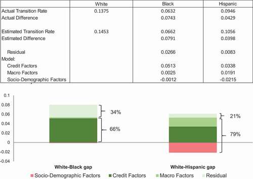
To summarize, Figure 2 presents the actual difference in the transition rate, the fitted difference in the transition rate (under pooled coefficients), and the contribution of sociodemographic, credit, and macro factors to the fitted difference. The residual effect is calculated as the unexplained portion of the estimated White–minority gap in transition rates. Credit factors alone explain 66–79% of this gap. For Hispanics, whereas sociodemographic factors alleviate the gap, macro factors significantly exacerbate the gap. The unexplained residual contributes 21–34% of the White–minority gap. The explanation for this residual gap is unclear, although it may be partly due to differences in factors such as assets, wealth, lender overlays, and consumers’ perceptions about required down payment (Goodman et al., 2017), which we cannot measure in our data.²⁷ For example, based on the National Survey of Mortgage Originations (NSMO), Blacks have slightly higher propensities than Whites to receive gifts and inheritance as a source of down payment.²⁸ However, we cannot observe the source of down payment in our data, which is most likely captured in the unexplained residuals of our models.

Figure 2. Decomposition of the racial/ethnic gap in the transition rate with respect to Whites. Authors' calculations using anonymized credit bureau data from 2012 and 2018

We perform several robustness checks on our baseline specification. Appendix E presents a detailed discussion of the findings from various alternative specifications. Our primary findings are consistent across all of these specifications.

4. Decomposition at the State Level

The U.S. economy is not a monolith, but an aggregate of geographically dispersed economies with varying business cycles. An analysis at the national level across a wide and diverse set of local areas may yield results that mute the effects of the diversity at the state level. Recognizing this, we examine to what extent the racial/ethnic gaps in the mortgage ownership rate persist at the state level and what the largest contributing factors are.

Panel A of Table 8 reports the racial/ethnic transition rates, the White–Black gap in transition rates, and results from the decomposition exercise for each state.²⁹ For accuracy, we report only the results for states with a Black population of more than 10,000 in our sample. For reference, we compute the national decomposition without including the state dummies, as reported in column 1.

Table 8. State-level Blinder–Oaxaca decompositions

Panel A. Decomposition of difference between Black and Non-Hispanic (NH) White transition rates into mortgage ownership
State name	U.S.	Alabama	California	Florida	Georgia	Illinois	Louisiana	Maryland	Michigan	Mississippi
Total	45,39,574	54,585	4,14,609	2,34,053	1,05,348	1,38,258	51,734	66,412	1,15,632	31,288
NH White	30,09,849	35,532	1,94,496	1,38,992	55,959	91,576	29,771	35,889	89,412	16,252
Black	5,13,398	16,371	14,392	30,009	36,414	17,048	17,858	18,340	14,630	13,688
NH White transition rate	0.15	0.13	0.12	0.13	0.14	0.16	0.13	0.18	0.16	0.12
Black transition rate	0.07	0.06	0.06	0.07	0.08	0.05	0.07	0.09	0.05	0.07
NH White-Black gap	0.08	0.07	0.06	0.06	0.07	0.11	0.07	0.08	0.12	0.05
Contributions from racial differences in:
Individual demographics	-0.02	-0.01	-0.01	-0.02	-0.01	-0.02	-0.02	-0.02	-0.02	-0.01
	0.00	0.00	0.00	0.00	0.00	0.00	0.00	0.00	0.00	0.00
	-22%	-20%	-11%	-37%	-20%	-16%	-24%	-23%	-20%	-17%
Household composition	0.01	0.01	0.01	0.01	0.01	0.01	0.01	0.01	0.02	0.00
	0.00	0.00	0.00	0.00	0.00	0.00	0.00	0.00	0.00	0.00
	12%	10%	9%	15%	12%	11%	12%	10%	13%	9%
Income growth	0.00	0.00	0.01	0.00	0.00	0.01	0.00	0.01	0.00	0.00
	0.00	0.00	0.00	0.00	0.00	0.00	0.00	0.00	0.00	0.00
	6%	2%	18%	-2%	0%	9%	4%	10%	2%	-1%
Education	0.00	0.00	0.00	0.00	0.00	0.00	0.00	0.00	0.00	0.00
	0.00	0.00	0.00	0.00	0.00	0.00	0.00	0.00	0.00	0.00
	2%	3%	2%	5%	3%	0%	4%	1%	1%	4%
Credit profiles	0.04	0.02	0.03	0.03	0.03	0.04	0.03	0.04	0.05	0.01
	0.00	0.00	0.00	0.00	0.00	0.00	0.00	0.00	0.00	0.00
	45%	36%	45%	58%	43%	39%	43%	52%	42%	21%
Severe derogatory credit	0.01	0.01	0.00	0.01	0.01	0.01	0.01	0.01	0.01	0.01
	0.00	0.00	0.00	0.00	0.00	0.00	0.00	0.00	0.00	0.00
	9%	18%	-1%	9%	12%	12%	17%	8%	11%	14%
Mortgage inquiries	0.01	0.01	0.01	0.01	0.01	0.01	0.01	0.01	0.01	0.01
	0.00	0.00	0.00	0.00	0.00	0.00	0.00	0.00	0.00	0.00
	11%	13%	16%	10%	11%	9%	15%	9%	9%	15%
Geography	0.00	0.00	0.01	0.01	0.01	0.00	0.00	0.00	0.00	0.01
	0.00	0.00	0.00	0.00	0.00	0.00	0.00	0.00	0.00	0.00
	2%	7%	10%	10%	8%	4%	2%	0%	3%	17%
Percentage explained by all variables	66%	70%	88%	68%	69%	68%	71%	67%	60%	63%
State Name	U.S.	New Jersey	New York	North Carolina	Ohio	Pennsylvania	South Carolina	Tennessee	Texas	Virginia
Total	45,39,574	1,03,723	2,12,868	1,07,975	1,36,912	1,45,006	56,275	74,483	2,83,400	92,375
NH White	30,09,849	62,726	1,28,583	69,781	1,09,936	1,13,548	34,202	57,096	1,46,233	58,416
Black	5,13,398	10,122	24,829	26,803	16,092	13,460	18,415	12,535	28,112	19,101
NH White transition rate	0.15	0.14	0.12	0.14	0.15	0.15	0.15	0.14	0.14	0.16
Black transition rate	0.07	0.06	0.04	0.07	0.06	0.06	0.07	0.07	0.06	0.09
NH White-Black gap	0.08	0.09	0.08	0.07	0.09	0.09	0.08	0.07	0.08	0.07
Contributions from racial differences in:
Individual demographics	-0.02	-0.02	-0.02	-0.01	-0.02	-0.02	-0.01	-0.02	-0.02	-0.01
	0.00	0.00	0.00	0.00	0.00	0.00	0.00	0.00	0.00	0.00
	-22%	-21%	-22%	-19%	-22%	-25%	-17%	-25%	-25%	-19%
Household composition	0.01	0.01	0.01	0.01	0.01	0.01	0.01	0.01	0.01	0.01
	0.00	0.00	0.00	0.00	0.00	0.00	0.00	0.00	0.00	0.00
	12%	13%	10%	9%	16%	15%	8%	17%	10%	8%
Income growth	0.00	0.01	0.00	0.00	0.00	0.00	0.00	0.00	0.01	0.01
	0.00	0.00	0.00	0.00	0.00	0.00	0.00	0.00	0.00	0.00
	6%	15%	2%	2%	-1%	-1%	6%	-1%	9%	10%
Education	0.00	0.00	0.00	0.00	0.00	0.00	0.01	0.00	0.00	0.00
	0.00	0.00	0.00	0.00	0.00	0.00	0.00	0.00	0.00	0.00
	2%	1%	1%	5%	0%	0%	8%	1%	4%	2%
Credit profiles	0.04	0.04	0.03	0.03	0.04	0.05	0.03	0.02	0.04	0.04
	0.00	0.00	0.00	0.00	0.00	0.00	0.00	0.00	0.00	0.00
	45%	44%	41%	48%	43%	50%	34%	36%	49%	53%
Severe derogatory credit	0.01	0.00	0.00	0.01	0.01	0.01	0.01	0.01	0.01	0.01
	0.00	0.00	0.00	0.00	0.00	0.00	0.00	0.00	0.00	0.00
	9%	4%	4%	12%	16%	12%	13%	21%	8%	10%
Mortgage inquiries	0.01	0.01	0.01	0.01	0.01	0.01	0.01	0.01	0.01	0.01
	0.00	0.00	0.00	0.00	0.00	0.00	0.00	0.00	0.00	0.00
	11%	10%	7%	13%	9%	9%	8%	13%	10%	12%
Geography	0.00	0.00	0.03	0.00	0.00	0.00	0.01	0.00	0.00	0.00
	0.00	0.00	0.00	0.00	0.00	0.00	0.00	0.00	0.00	0.00
	2%	5%	41%	1%	0%	5%	8%	4%	2%	3%
Percentage explained by all variables	66%	70%	84%	72%	60%	63%	68%	67%	67%	79%
Panel B. Decomposition of difference between Hispanic and Non-Hispanic White transition rates into mortgage ownership
State Name	U.S.	Arizona	California	Florida	Illinois	New Jersey	New York	Texas
Total	45,39,574	63,912	4,14,609	2,34,053	1,38,258	1,03,723	2,12,868	2,83,400
NH White	30,09,849	41,962	1,94,496	1,38,992	91,576	62,726	1,28,583	1,46,233
Hispanic	6,72,294	15,808	1,42,256	53,259	18,792	17,954	33,866	90,735
NH white transition rate	0.15	0.15	0.12	0.13	0.16	0.14	0.12	0.14
Hispanic transition rate	0.11	0.13	0.10	0.12	0.13	0.09	0.06	0.10
NH white-Hispanic gap	0.04	0.01	0.02	0.01	0.03	0.05	0.06	0.04
Contributions from racial differences in:
Individual demographics	-0.02	-0.02	-0.01	-0.02	-0.03	-0.02	-0.02	-0.03
	0.00	0.00	0.00	0.00	0.00	0.00	0.00	0.00
	-61%	-206%	-50%	-278%	-112%	-46%	-33%	-62%
Household composition	0.00	0.00	0.00	0.00	0.00	0.01	0.00	0.00
	0.00	0.00	0.00	0.00	0.00	0.00	0.00	0.00
	6%	16%	-7%	45%	5%	10%	6%	0%
Income growth	0.00	0.00	0.01	-0.01	0.00	0.00	0.00	0.00
	0.00	0.00	0.00	0.00	0.00	0.00	0.00	0.00
	-7%	5%	24%	-81%	-3%	7%	2%	6%
Education	0.00	0.01	0.00	0.00	0.00	0.00	0.00	0.01
	0.00	0.00	0.00	0.00	0.00	0.00	0.00	0.00
	8%	44%	19%	44%	-4%	1%	3%	25%
Credit profiles	0.03	0.03	0.02	0.02	0.03	0.03	0.02	0.03
	0.00	0.00	0.00	0.00	0.00	0.00	0.00	0.00
	70%	270%	85%	213%	118%	59%	38%	72%
Severe derogatory credit	0.00	0.00	0.00	0.00	0.01	0.00	0.00	0.00
	0.00	0.00	0.00	0.00	0.00	0.00	0.00	0.00
	10%	29%	0%	27%	27%	4%	2%	10%
Mortgage inquiries	0.00	0.00	0.00	0.00	0.00	0.01	0.01	0.01
	0.00	0.00	0.00	0.00	0.00	0.00	0.00	0.00
	7%	36%	16%	18%	6%	10%	10%	14%
Geography	0.01	0.00	0.01	0.01	0.01	0.01	0.04	0.00
	0.00	0.00	0.00	0.00	0.00	0.00	0.00	0.00
	33%	7%	23%	170%	28%	25%	60%	7%
Percentage explained by all variables	66%	-	-	-	66%	72%	87%	71%

Note. Each row gives the coefficient, standard error (in parentheses), and percentage contribution by each category of variables to the racial/ethnic difference in transition gap. The first column gives the national decomposition results, excluding state dummies, in the regression analysis. For states with a small racial/ethnic gap, such as Arizona, California, and Florida, the decomposition exercise is hard to interpret. Hence, the group differences in all included characteristics are not reported.

First, in Maryland and Virginia, both Whites and Blacks are transitioning to new mortgages at a higher rate than the national average. Second, whereas states such as California, Florida, and Mississippi have a White–Black gap in the transition rate that is lower than the national average, states such as Illinois, Michigan, New Jersey, Ohio, and Pennsylvania have White–Black gaps in the transition rate higher than the national average. For example, the racial/ethnic gap in the transition rate in Illinois and Michigan is 11% and 12%, respectively, significantly higher than the national gap of 8%. For almost all states (except Mississippi), credit profiles explain most of the gap, followed by household composition, severe derogatory credit, and mortgage demand. Compared with the national case, the racial/ethnic disparity in income matters substantially more in explaining the racial/ethnic gap for California, Maryland, New Jersey, Texas, and Virginia. Furthermore, in contrast to the national case, geography explains a significant portion of the White–Black gap for New York, Mississippi, California, and Florida. This may be partly because of lower affordability, and partly because of the higher unemployment rates of Blacks residing in these states. For instance, the affordability index for Blacks is significantly higher than that of Whites in New York (1.60 vs. 1.15), indicating that Blacks are concentrated in urban and more expensive pockets within the state. In contrast, the local unemployment rate is substantially higher for Blacks compared with Whites in Mississippi (10.0% vs. 8.5%), making it harder for Blacks to obtain financing for mortgages locally.

Panel B of Table 8 reports the racial/ethnic transition rates, the White–Hispanic gap in transition rates, and results from the decomposition exercise for eight states with a Hispanic population of more than 10,000 in our sample. Column 1 reports the national decomposition calculated without including state fixed effects in the regression model, for reference. Whereas New York and New Jersey have a higher than national average White–Hispanic gap in transition rates, states such as Arizona, California, and Florida have a negligible gap in transition rates.³⁰ Similar to the national case, whereas racial/ethnic disparities in credit profiles play an important role in increasing the racial/ethnic gap in transition rates for most states, racial/ethnic differences in individual demographics shrink the gap. In contrast to the national case, income disparity contributes positively to the racial/ethnic gap in New Jersey, New York, and Texas. Lastly, geography follows an interesting trend. On one hand, it contributes 60% of the gap in New York, which is substantially higher than the national case. The affordability indices for Hispanics and Whites in New York are 1.65 and 1.15, respectively, suggesting that Hispanics are living in cities, suburbs, and exurbs within the state, making it harder for them to afford a mortgage. On the other hand, geography contributes only 7% of the White–Hispanic gap in Texas, which is significantly lower than the national average. The affordability indices for Hispanics and Whites in Texas are 0.67 and 0.69, respectively, indicating that typically, Hispanics are not living in less affordable areas compared with Whites within the state.

In a nutshell, the state-level decomposition exercise reveals considerable heterogeneity within the nation. For example, our findings suggest that geography is a less important barrier to mortgage ownership for Blacks nationally. This is driven by a lower contribution of geography to the White–Black gap in transition rates for most states, which offsets the significantly higher contribution of geography to the White–Black gap in the transition rate in New York and Mississippi. The distribution of income, unemployment, and house prices at the more local level may affect the propensity for mortgage ownership of both minority groups.

5. Conclusion

During the Great Recession and the subprime lending crisis, Black and Hispanic homeowners were disproportionately affected by foreclosures and the tighter lending standards. New HMDA-reported mortgage originations to Black and Hispanic borrowers declined from 25% of originations in 2006 to just 12% by 2009. As of 2018, the White–Black and White–Hispanic mortgage ownership gaps stood at roughly 17 and 16 percentage points, respectively. At the same time, the White–Hispanic and White–Black homeownership rate gaps persisted. This study uses uniquely constructed credit bureau data to answer two questions: How do consumers’ credit profiles determine their decision to enter mortgage ownership? What explains the racial/ethnic gap in rates of transition to obtaining new mortgages?

Our research reveals several interesting findings. First, using a logistic regression model, we find that some of the important determinants of the decision to enter mortgage ownership are age, income growth, marital status, getting a FICO score, the individual’s demand for a mortgage, and local unemployment rates. Consumers with limited credit histories are less likely to transition to acquiring new mortgages. Other factors, such as student loan debt, auto debt, gender, number of children, and educational attainment, play less important roles.

Second, we find that Blacks are one half, and Hispanics are two thirds, as likely as Whites to transition to mortgage ownership in our sample. To allow the impact of credit-related factors to differ, we investigate the racial/ethnic gap in transition rates separately for Black and Hispanic consumers. Using the Blinder–Oaxaca decomposition technique for nonlinear equations, we find that racial/ethnic differences in the distribution of credit attributes explain a large part of the racial/ethnic gap in the rate of transition to mortgage ownership. Specifically, both minority groups have lower credit scores and higher delinquencies, and are more likely to have missing credit scores, than Whites—all of which contribute to the lower average probabilities of entering mortgage ownership for minorities than Whites. We anticipate that this effect may be amplified if lenders are imposing tighter credit standards to minimize rep and warrants risk. The lower credit profiles of Black and Hispanic consumers compared with Whites also, we suggest, explains a large part of the racial/ethnic gap in the homeownership rate.

We also find two key differences between the factors explaining the White–Black and White–Hispanic gaps in transition rates. First, whereas geography matters substantially in explaining the White–Hispanic gap nationally, it explains virtually none of the White–Black gap nationally. Recognizing that decomposition at the national level may mute local effects, we conduct a state-wise decomposition exercise to better understand factors contributing to local homeownership gaps. We find that there is considerable heterogeneity across states, especially regarding the contribution of geography. For example, geography can be an important barrier to homeownership for Blacks residing in New York, mainly because they are concentrated in the city centers or suburbs. This implies the need for strategies that support more employment opportunities, improve access to credit and availability of low-down payment programs, and increase the elasticity of housing supply, driving down prices and improving affordability.

Second, racial/ethnic differences in household composition contribute more in explaining the White–Black gap relative to the White–Hispanic gap. Although lenders are not able to directly influence potential mortgage borrowers in terms of factors such as family structure, including marriage and children, they should be aware of differences and the extent to which credit policies may interact with these differences. Overall, our analysis cannot account for about 33–35% of the White–Black gap and 7–28% of the White–Hispanic gap, which could be due to differences in institutional factors, assets, and wealth.

Our findings suggest that consumers with missing FICO scores and thin files are less likely to qualify for mortgages. Alternative credit data, such as telecom, utility, and rental information, might more accurately identify credit-worthy consumers with missing FICO scores or thin files. Goodman and Zhu (2018) make the case for the inclusion of rental payments in assessing mortgage applications. They compare rental payments with mortgage payments by income level while demonstrating that past mortgage payment history helps predict future loan performance.

Increased funding for programs intended to educate potential minority homeowners to use credit as a tool would be worthwhile. Our results indicate applying the credit profile distribution of White consumers to the Black consumers in our sample would increase the predicted mortgage entry rates of Black consumers by an amount equivalent to roughly 66–79% of the observed gap in mortgage entry rates between Whites and Blacks. Counseling and credit education opportunities could help place minorities in a better position to qualify for a mortgage. It also critical to ensure that homeowners have sustainable mortgages that are less likely to result in default or foreclosure. The use of prepurchase counseling is not universal, and studies suggest it is beneficial. Argento et al. (2019) estimate that 17% of first-time homebuyers receive some form of homebuyer education or counseling. The reported take-up rate was higher for Blacks in their sample, at 41%. Those who report counseling are more likely to report better mortgage knowledge. Peck, Moulton, Bocian, Demarco, and Fiore (2019) find that participants randomly assigned to a homebuyer education and counseling program were more likely to have a credit score of 620 or higher after the program. They also find that participants were more likely to say they would contact a counseling agency or nonprofit prior to missing a mortgage payment, that they were confident that they could find information they needed and were more likely to set up auto payments for their mortgage payments.

Low and no down payment programs backed by enterprises, Ginnie Mae, and state and local housing finance agencies can help overcome the geographic barriers. Furthermore, to the extent that the residual gap is explained by differences in parental wealth (see Hilber and Liu 2008), low and no down payment programs may also help overcome the unexplained residual gap.

Lastly, it would be beneficial for the federal government to provide assistance, such as modifications, payment deferrals, or forbearance, for low-income and minority existing homeowners to stay in their homes. Moulton et al. (2019) find that mortgage payment assistance programs to shield against income shocks, such as the Hardest Hit Fund, can significantly reduce the risk of default of the low-income and vulnerable population. A combination of strategies supporting counseling and credit education opportunities, income and wealth creation, and debt rehabilitation will likely be the most effective in bridging the homeownership gap between Whites and minorities over time.

Acknowledgments

We thank Robert Avery, Laurie Goodman, Raphael Bostic, Steve Ross, Stephanie Moulton, Jaclene Begley, Timothy Lambie-Hansen, Douglas McManus, Cynthia Waldron, Sam Khater, Leonard Kiefer, and Sijie Li for helpful feedback, as well as the participants of the 2019 Urban Economics Association Meeting, 2019 FDIC Economic Inclusion Advisory Committee Meeting, 2019 APPAM Meeting, 2019 Southern Economics Association Meeting, 2019 Urban Institute Data Talk, and Freddie Mac Brown Bag series. This article also benefitted from the input of three anonymous reviewers. The analysis and conclusions in this article are those of the authors and do not necessarily reflect the views of Freddie Mac.

Disclosure Statement

No potential conflict of interest was reported by the authors.

Additional information

Notes on contributors

Jaya Dey

Jaya Dey is a senior economist in the Single-Family Client and Community Engagement division of Freddie Mac. Her area of research is housing policy, with a focus on affordability, access to credit and changing demographics. Prior to arriving at Freddie Mac, she was an assistant professor of economics at Oklahoma State University and a visiting faculty member at Saint Louis University. She holds a PhD in economics from The Ohio State University and a master’s degree from the Indian Statistical Institute, New Delhi.

Lariece M. Brown

Lariece Brown is a senior economist and quantitative analytics director in the Single-Family Client and Community Engagement division of Freddie Mac. She leads a team conducting analytics of and research on underserved markets. She has extensive experience in research to support fair lending, affordable lending, and assessing opportunities to expand access to credit. She has also served as a senior financial economist and section chief with the Federal Deposit Insurance Corporation. She earned her MA in mathematics and PhD in economics from The Ohio State University.

Notes

1. Some economists expect the homeownership rate to decline even further (see Acolin, Goodman, & Watcher 2016; Goodman, Pendall, & Zhu, 2015; Nelson, 2016), whereas others hypothesize that changing demographics will slowly increase the homeownership rate (see Haurin, 2016).

2. The White–Black homeownership gap increased from 28 percentage points in 2007 to 31 percentage points in 2018, according to the U.S. Census Housing Vacancy Survey. The White–Hispanic homeownership rate gap was 26 percentage points in 2007 and 2018.

3. The calculations are for owner-occupied mortgages.

4. We use the ACS PUMS to define individual-level estimates that only identify the household head and spouse as the homeowners, excluding adult children and other adults living in the household. See Appendix A for detailed discussion of our methodology.

5. The CRA, passed in 1997, targets regulated and insured financial institutions and mandates increased mortgage lending in underserved areas. Similarly, the GSE Act, passed in 1992, mandates Fannie Mae- and Freddie Mac-increased purchases of conforming loans in underserved communities. See Gabriel and Rosenthal (2008) for details.

6. The existing literature explores the role of student loan debt in economic well-being and homeownership rates (Fry, Parker, & Rohal, 2014; Mezza et al., 2016). Although richer data are needed to address this issue, our findings suggest that student loan debt has minimal impact on the mortgage ownership rate.

7. Under rep and warrants risk, if the guaranteed loans sold to GSEs default within a given period, GSEs or the Federal Housing Administration will ask the lenders to repurchase it. See Acolin, Goodman, and Wachter (2019).

8. Previous studies have shown married couples are much more likely to be homeowners than unmarried individuals are, because of their generally better socioeconomic status. Dual incomes increase the affordability and accessibility of homeownership for partnered versus single-person households (Drew, 2015; Haurin, Hendershott, & Wachter, 1996; Hendershott, Ong, Wood, & Flatau, 2009). Married couples are also more likely to have children and therefore more likely to desire both large dwellings and locations in neighborhoods close to family-friendly amenities and better schools (Clark & Davies Withers, 2007).

9. For example, Wainer and Zabel (2019) find that low-income households that owned their homes during a period of relative stability enjoyed significant gains in wealth, whereas those households that purchased and owned their houses during a period of relative volatility, such as the Great Recession, experienced little gain in wealth.

10. Bartlett et al. (2019) also warn that statistical biases may still be present in automated algorithms, especially in pricing.

11. Using names and addresses to model race and ethnicity has been done by others, such as the Consumer Financial Protection Bureau. See https://files.consumerfinance.gov/f/201409_cfpb_report_proxy-methodology.pdf

12. We did not include change in FICO score from 2012 to 2018 or FICO score in 2018, because they can be endogenous with obtaining new mortgages by 2018.

13. Estimated tax-reported income is at the pretax level and may include spousal income if taxes are filed jointly. Because we are using income and DTI growth rates, their value levels in two time periods is less relevant.

14. Back-end DTI indicates what percentage of consumer’s gross monthly income goes into paying recurring monthly debt, including mortgage payments (principal, interest, taxes, and insurance).

15. Appendix B, Figure B8 plots the percentage of consumers with clean thin files by age cohort. The figure reveals that the share of population with thin files has a U-shaped pattern with age: it is highest for young millennials, falls with age and then rises again for consumers above 55 years old. Moreover, Hispanics are more likely to have thin files compared with non-Hispanic Whites. This finding is consistent with a recent study done by Brevoort et al. (2015), who find that Blacks and Hispanics are more likely than Whites or Asians to be considered unscorable or credit invisible. A possible explanation for this discrepancy is that Hispanics are skewed younger than the overall population, and a large share of this population comprises recent immigrants with insufficient credit histories.

16. Note that not all of those who inquired about a mortgage in 2012 have a mortgage by 2018.

17. The estimation sample includes the individuals with nonmissing values for certain key independent variables in our model.

18. The indefinite/uncertain category of gender refers to cases where the name could be either male or female, so the classification is unclear. In our overall estimation sample, this category comprises around 0.08%. We maintain this as a separate category throughout our estimation.

19. The coefficients reported in the multivariate results tables are marginal probabilities with t values given in parentheses, instead of logit coefficients. The marginal propensities are obtained by calculating the observation-level marginal effect and then averaging across the observations. For categorical variables, the effect is the discrete first difference from the reference category (Stata v. 15 documentation for margins, dydx). The raw regression results for all model specifications are available from the authors on request.

20. Models 1–4 include different categories of credit attributes. Since these four specifications conducted on our estimation sample use only credit bureau data, they have the same number of records: 2,460,975. Model 5, which is our baseline model, includes the macroeconomic and geographic variables, such as county-level house price and unemployment rates. These variables were separately merged to our credit bureau data and have missing observations for a few counties, reducing the number of observations in Model 5 to 2,347,247.

21. Miller and Park (2016) find that the legal recognition of same-sex marriage is associated with an increase in home purchase mortgage applications from same-sex applicants of 7–13%. The results vary by the timing of the state’s recognition of same-sex marriage relative to the federal-level repeal of the Defense of Marriage Act.

22. A possible explanation for the small impact of credit scores is that they are highly correlated with income. In our sample, the correlation between consumers’ FICO score and income series is 0.50.

23. In Appendix E, we run a robustness check where we consider a single indicator of whether FICO is missing in 2012. Both the likelihood ratio test and the pseudo R² suggest a lower fit compared with our baseline case.

24. The existing literature explores the role of student loan debt in economic well-being and homeownership rates, especially of young adults (Fry et al., 2014; Mezza et al., 2016). Using the instrumental variables approach, Mezza et al. (2016) find that a $1,000 increase in student debt loan accumulated before age 23 is associated with a decrease of 1.5 percentage points in the probability of homeownership. Miller and Nikaj (2018) estimate that a 10% increase in the amount of student loan debt is associated with a decrease of 0.3 percentage points in the probability of homeownership. Our findings suggest that student loan debt, although significant, has only a small effect on transition probability.

25. See Fairlie (1999) for details. The Statistical Analysis System (SAS) codes from the original article are uploaded: https://people.ucsc.edu/~rfairlie/decomposition/

26. Krimmel (2018) shows that HOLC overwhelmingly marked black neighborhoods for credit redlining in 1940, which in turn affected neighborhood quality through both supply and demand channels. On the supply side, this regulation restricted access to credit, mortgage insurance, and new home construction in these neighborhoods. On the demand side, it slowed down housing demand in these neighborhoods as families fled for nonredlined neighborhoods. His findings suggest that HOLC ratings caused declining housing supply and population density in the redlined tracts for decades thereafter.

27. Lenders may impose additional overlays if consumers experienced recent bankruptcies, making it harder for them to transition to new mortgage ownership. Although credit overlays could be present, we are not able to observe them in our matched credit bureau data.

28. In Appendix D, we include a table based on NSMO, which indicates that Blacks rely more than Whites on savings, inheritance, gifts, and grants from family or friends to meet their down payment requirements. The public-use data files are available at https://www.fhfa.gov/nsmodata

29. We only report the decomposition exercise calculated at the pooled coefficients. The coefficient estimates are based on state-level logistic regressions.

30. For states with a small racial/ethnic gap, such as Arizona, California, and Florida, the decomposition exercise is hard to interpret. Hence, the group differences in all included characteristics are not reported.

31. The 2016 ACS estimates for the age cohorts 18–35, 36–55, and 55+ are approximately 32%, 34%, and 35%, respectively.

32. To better understand the implications of this data limitation, we ran a robustness check on our benchmark specification by dropping all records with missing age. Our results are robust to this alternative specification. Please see Appendix E for details.

33. Most of these fragment files get dropped in our estimation sample, which focuses on consumers that are observed in both 2012 and 2018. See Table 1.

34. In Appendix A, we discuss our detailed methodology, comparison, and limitations.

35. The shape of the curve and percentages are consistent with a recent report published by the Urban Institute: https://www.urban.org/research/publication/americans-debt-styles-age-and-over-time

36. The life cycle of foreclosures is largely consistent with New York Fed’s quarterly report on household debt and credit: https://www.newyorkfed.org/medialibrary/interactives/householdcredit/data/pdf/HHDC_2016Q1.pdf

37. Our matched credit bureau data do not include information on origination date or origination loan amount. We are only able to observe the size of the outstanding balance at the time the data were pulled. Without knowing the origination loan amount, just observing the size of the mortgage close to transitions out of mortgage ownership will not inform us about the disposition of the outstanding mortgages.

38. See https://www.fhfa.gov/nsmodata for additional information on the NSMO.

39. There are two reasons why we consider those 55 and younger as new mortgage owners. First, Argento et al. (2019) analyze first-time homebuyers’ counseling and mortgage selection experience using the National Sample of Mortgage Originations. They restrict their analysis to homebuyers younger than 55 to increase the likelihood that the analysis is focused on first-time buyers rather than those who have paid off their mortgages. Second, Figure A1 in Appendix A suggests mortgage ownership typically follows an inverted-U age pattern: it rises with age until the mid-50s and then falls as consumers move to older age groups and are more likely to own their house free and clear. Based on these two lines of evidence, our subsample of consumers 55 and younger are more likely to be first-time homebuyers.

40. By using the transition variable in the baseline case, we are able look more closely at the group with a missing FICO score in 2012 to understand why they appear more likely to obtain a new mortgage. We find that this is driven by those who were able to generate a credit score by 2018. The individuals we observe with a credit score in 2018 but not 2012 are likely to be younger minorities (see Table 2). These individuals could be those taking steps to move into homeownership or increasing their demand for credit in general, which could put them in a better position to obtain a mortgage.

Appendix A.

Defining the Individual-Level Mortgage Ownership Rate in the American Community Survey

The mortgage ownership rate in our credit bureau data is only about one third of the homeownership rate from the American Community Survey public-use microdata (ACS PUMS) in 2018 (30.4% vs. 64.4%). Mortgage ownership rate and homeownership rate are different measures, for at least three reasons.

First, the homeownership rate from ACS PUMS is defined at the household level, whereas the mortgage ownership rate is defined at the individual level. For example, an adult child living with parents in an owner-occupied housing unit or a student renting a room from a homeowner would be identified as a homeowner according to ACS PUMS but would not be considered a mortgage owner in credit bureau data (see Goodman & Li, 2016). Second, our credit bureau data cannot identify the tenure status of individuals. Whereas older consumers are more likely to pay off their mortgage debt and own their houses free and clear, a substantial number of younger consumers purchase homes with cash or receive them as an inheritance. According to the 2017 ACS, about 4% of owners of owner-occupied housing units originally received their homes as a gift or inheritance, and among those who purchased their own homes, about 12% paid cash. Limiting the sample to first-time homeowners, these figures become about 5% and 9%, respectively. These consumers will be counted as homeowners according to ACS PUMS but not mortgage owners according to our matched credit bureau data. Lastly, our data likely underrepresent people who do not interact with the credit system, including immigrants and younger consumers.

Nonetheless, to make the ACS PUMS definition of an owner consistent with the one in our credit bureau data, we create an individual-level ownership status for each person in ACS PUMS following Goodman and Li (2016). First, an owner must be an adult (age 18 or older) living in an owner-occupied housing unit who is either the head of the household or the spouse of the head of the household. We exclude adult children and other adults living in the household (renters, students, or relatives) as owners. Using this approach, we compute homeownership rate at the individual level. Second, to capture mortgage owners in ACS PUMS, we include only those homeowners who own a house with a mortgage or loan. In this way we purge the consumers who own their houses free and clear and cannot be identified in our credit bureau data.

Figure A1 plots the individual homeownership and mortgage ownership rates by age cohort using our definition and 2018 ACS PUMS 1-year estimates. As the figure suggests, homeownership rate typically rises with age until 77, after which it declines. Consumers older than 77 are more likely to downsize, live with children, or live in assisted living facilities. Mortgage ownership typically follows an inverted-U age pattern: it rises with age until mid-50s and then falls as consumers move to older age groups, since they are more likely to own their house free and clear.

Figure A1. Individual-level homeownership rate and mortgage ownership rate in ACS PUMS (2018). Authors' calculations using 2018 ACS PUMS 1-year estimates

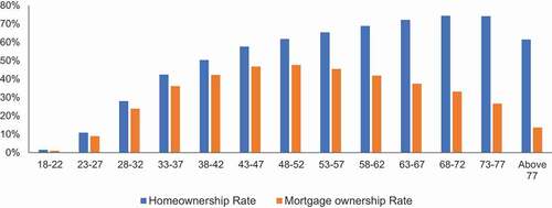
Table A1 presents the individual-level homeownership rate and mortgage ownership rate by race/ethnicity over 2008–2018. According to the table, around 49% and 31% of the adult population overall are homeowners and mortgage owners, respectively, in 2018. This implies that around 52% are renters, 18% (49–31 = 18) own a house free and clear, and 31% own a house with a mortgage or loan. This number is reasonably close to the number calculated using our credit bureau data, which show that 30% of adult consumers are mortgage owners in 2018.

Table A1. Homeownership and mortgage ownership rate at the individual level (%)

	Homeownership rate (individual level)				Mortgage ownership rate (individual level)
Year	Overall (%)	NH White (%)	Black (%)	Hispanic (%)	Overall (%)	NH White (%)	Black (%)	Hispanic (%)
2008	52.7	60.9	32.5	33.4	37.0	41.6	24.9	26.2
2009	51.9	60.3	31.7	32.2	36.2	40.9	24.1	24.9
2010	51.1	60.0	31.2	31.2	35.3	40.3	23.5	23.9
2011	50.1	59.1	30.5	30.5	34.3	39.3	22.7	23.0
2012	49.4	58.5	29.7	30.1	33.5	38.6	21.9	22.4
2013	48.8	57.8	29.2	29.5	32.3	37.3	21.1	21.2
2014	48.3	57.6	28.6	29.3	31.7	36.9	20.5	20.9
2015	48.2	57.6	28.4	29.6	31.4	36.6	20.1	20.8
2016	48.2	57.6	28.3	29.7	31.3	36.6	19.8	20.6
2017	48.8	58.2	28.8	30.8	31.6	36.9	20.1	21.3
2018	49.0	58.6	29.0	31.2	31.2	36.6	20.0	21.0

Note. NH = Non-Hispanic. ACS PUMS 1-year estimates.

Our credit bureau data likely have two sources of undercounting of mortgage owners. First, according to our definition, if a spouse is not a coborrower on the mortgage, the spouse is counted as a nonmortgage owner in our credit bureau data but as an owner in ACS PUMS. Second, home loans taken out for the purchase of manufactured housing do not necessarily show up in credit bureau data as mortgage credit lines (see Critchfield, Dey, Mota, & Patrabansh, 2019). Nationwide, manufactured housing accounts for around 6% of occupied housing (CFPB, 2014). More than 80% of manufactured housing units are titled as personal property, and about half are purchased with cash. Those that are financed primarily involve personal property loans, and are more likely to show up in credit bureau data as auto loans or other miscellaneous debt than as mortgages. In contrast, owners of manufactured housing who purchased with loan will be considered mortgage owners in ACS PUMS regardless of their type of financing.

One caveat is that the propensities for homeownership and mortgage ownership can differ systematically across racial/ethnic groups. For example, the housing structure type differs across these groups, on average, with Whites more likely to own the single-family detached properties that tend to carry a traditional mortgage and Hispanics more likely to own manufactured housing, which is underrepresented in credit data. However, these differences are minor and do not explain the White–minority gap in mortgage ownership rate that remains substantial over the decade. Furthermore, this article aims to define changes in mortgage ownership status, or transition rates, which capture the inflow/outflow of mortgage ownership and are less affected by the stock of mortgage ownership at a given point in time.

Appendix B.

Summary Statistics of the Matched Credit Bureau Data (2016)

The credit bureau panel data were constructed as a random sample of the credit-visible population in 2016. For everyone in our panel, we have individual- and household-level information for 2012, 2016, and 2018. Table B1 presents the frequencies and median values of individual-level and household-level variables in the sample for 2016, when our sample was drawn. It also reports similar statistics for the adult population from 2016 American Community Survey public-use microdata (ACS PUMS) 1-year estimates. The median age of consumers in our sample is 50, which is higher than the median age reported in the ACS (46). This disparity occurs mainly because our population with credit records is skewed older, with only adult credit-visible consumers. As the table suggests, 21% of consumers in our data are 18–35 years of age, 28% of consumers are 36–55, and another 28% are older than 55, which is systematically lower than the ACS estimates.³¹ Information on age is missing for 23% of our population. An explanation for consumers with missing age is the existence of fragment files in credit bureau data—that is, some consumers having multiple credit records containing a portion of the consumer’s credit histories that exist outside their primary file (Brevoort, Grimm, & Kambara, 2015). Over time, as more information becomes available, the National Credit Rating Agency may determine that these fragment files belong to a consumer with an existing credit record. Consequently, the information from the fragment files is merged into the consumer’s primary credit record, and the fragment files disappear. By using data from 2012 and 2018, we are able to construct a more complete picture of the consumers’ credit records. This helps us work around the fragment files in our estimation sample, which focuses on consumers that are observed in both 2012 and 2018. Note that the summary statistics for our estimation sample (see Table 1) indicate it is missing ages for only 5% of the observations.³²

The percentages of non-Hispanic White, Hispanic, and Black consumers in our sample are 63.2%, 16.9%, and 11.7%, respectively, values that are very similar to the ACS estimates of 64.1%, 15.7%, and 12% of non-Hispanic Whites, Hispanics, and Blacks, respectively. Other race/ethnicities, comprising Asians, Pacific Islanders, and Native Americans, constitute 6% of our sample. As shown in Table B1, the percentages of male and female consumers are both around 41%, which are lower than the ACS estimates of 49% and 51%, respectively. The gender of around 5% of our consumers is unknown and is likely to be distributed evenly across male and female. Furthermore, the percentage of married consumers is 48%, which is consistent with the ACS estimates. The percentage of the sample population with at least a high school diploma in 2016 is 74%, and that with at least a bachelor’s degree in 2016 is 23%, lower than the ACS estimates of 87% and 29%, respectively. Information on gender, marital status, and education is missing for 12% of our sample, partly because there was no match between these consumers’ credit database and marketing data, and partly because they are fragment files.³³ Next, the median tax-reported income in our data is $64,000, which is slightly higher than the median family income in ACS because our sample is restricted to the credit-visible population, who tend to have higher income. Except for the Other race category, median tax-reported income for all race/ethnicity is similar to its ACS counterpart.

Table B1. Comparison with the American Community Survey

Characteristics	2016 Credit Bureau Data	2016 ACS PUMS 1-year estimate (ages 18 and above)
Age
18 ≤ age ≤25	6.10%	14.34%
26 ≤ age ≤ 35	15.05%	17.65%
36 ≤ age ≤ 45	13.66%	16.36%
46 ≤ age ≤ 55	14.00%	17.14%
56 ≤ age ≤ 65	12.90%	16.21%
66 ≤ age ≤ 70	5.05%	6.35%
Above 70	9.83%	11.94%
Missing	23.43%	-
Median Age	50	46
Race/ethnicity
Non-Hispanic White	63.20%	64.11%
Black	11.69%	11.98%
Hispanic	16.87%	15.66%
Other	6.09%	6.54%
Missing	2.15%	-
Gender
Male	41.09%	48.64%
Female	41.02%	51.36%
Unknown	5.74%	-
Missing	12.00%	-
Marital status
Married	47.53%	49.89%
Single	17.95%	50.11%
Unknown	22.53%	-
Missing	12.00%	-
Education
High school dropout	12.37%	12.64%
High school diploma	26.10%	27.63%
Some college	24.86%	30.95%
Bachelor’s degree	14.47%	18.21%
Graduate degree	8.25%	10.57%
Unknown	1.95%	-
Missing	12.00%	-
Median income ($)
Overall	64,000	63,900
Non-Hispanic White	71,000	70,000
Black	45,000	47,200
Hispanic	49,000	50,300
Other	68,000	80,000
Mortgage ownership
Overall	25.96%	31.30%
Non-Hispanic White	30.85%	36.64%
Black	14.76%	19.83%
Hispanic	16.79%	20.57%
Other	22.34%	27.76%

Note. Credit bureau (2016) and ACS PUMS (2016). Other includes Asian, Native American, and Pacific Islander. The race/ethnicity categories are mutually exclusive.

Lastly, our credit bureau data include the total number of open mortgage-type trade lines reported in the previous 6 months. This attribute allows us to track individual-level mortgage ownership status in 2016. Using this attribute, we calculate the mortgage ownership rate at the individual level for the overall population and by race/ethnicity. As the table suggests, the overall mortgage ownership rate in 2016 is around 26%. Whereas for non-Hispanic Whites mortgage ownership rate is around 31%, for the two minority groups it is between 15% and 17%. For comparison, we compute the ACS counterpart of the individual mortgage ownership rate.³⁴ Based on our methodology, the overall mortgage ownership rate in the 2016 ACS is around 31%, which is reasonably close to the estimates in our sample. Note that the estimates of mortgage ownership rate are slightly lower in our sample compared with the ACS PUMS. This is likely because the credit bureau data undercount mortgage owners. For example, if a spouse is not a coborrower on the mortgage, the spouse is counted as a nonmortgage owner in our sample but as an owner in ACS PUMS according to our definition (see Appendix A).

Next, we describe various credit attributes of our primary sample by age cohort in 2016. We look at the distribution of credit scores, DTI measures, foreclosures, and bankruptcies by age and race/ethnicity. Figure B1 plots the median FICO score in 2012 by age cohort for the overall population (black line), non-Hispanic Whites (gray line), Hispanic population (orange line), and Black population (blue line). The median FICO score typically rises with consumers’ age as people tend to become more credit established with age. Whereas non-Hispanic Whites tend to have higher credit scores than the overall population across all age groups, Black and Hispanic consumers tend to have lower median credit scores compared with the overall population.

Panel A of Figure B2 plots the percentage of consumers with any debt in 2016. More non-Hispanic Whites in their 50s and 60s have debt, compared with the others. Panel B plots the median total debt (in dollars) in 2016 by age cohort for each demographic. The median debt balance typically follows an inverted-U age pattern: it increases from $15,000 in consumers’ mid-20s to $50,000 in consumers’ 30s and 40s, and then declines to $4,000 in the mid-70s, for the overall population. For most age cohorts, non-Hispanic Whites have higher median debt than the overall population, whereas both minority groups have lower median debt than the overall population.

Panel A of Figure B3 plots the percentage of consumers with some student loan debt in 2016. Around 10% of the overall population has student loan debt. More consumers in their 20s and 30s have student loan debt.³⁵ For all age cohorts, fewer Hispanics have student loan debt compared with non-Hispanic Whites. Whereas fewer Blacks in their 20s have student loan debt compared with Whites, more Blacks in their 40s have student loan debt compared with Whites. Panel B, which plots the median student loan debt in dollars for those who have student loan debt, shows that median debt is lower for minorities compared with non-Hispanic Whites for almost all age cohorts.

Panel A of Figure B4, which plots the percentage of consumers with some credit card loan debt in 2016, shows that fewer Blacks and Hispanics have credit card debt compared with non-Hispanic Whites. Panel B shows that the median credit card debt is lower for Hispanics and Blacks than for non-Hispanic Whites.

Panel A of Figure B5, which plots the percentage of consumers with auto trades in 2016, shows that fewer minorities in their 20s through 50s have auto debt compared with non-Hispanic Whites. Panel B shows that whereas median auto debt is higher for Hispanics compared with Whites for the younger and older population, it is higher for Blacks compared with Whites only for the older population.

Figure B6 and Figure B7 plot the percentage of consumers with any foreclosures in the last 84 months (since September 2016) and any bankruptcies in the last 84 months (since September 2016), respectively. The figures show that the relationship of foreclosures and bankruptcies with age follows an inverse U-shaped pattern: they rise with age and then fall as consumers move to older age groups.³⁶ In addition, both minority groups in older age cohorts tend to have more foreclosures and bankruptcies than non-Hispanic Whites do.

Lastly, Figure B8 plots the percentage of consumers with so-called thin files and with clean credit records by age cohort. We define consumers with thin files and with clean credit records as those with few trade lines (two or fewer) reported in their credit records and no delinquencies in the last 180 days, no foreclosures in the last 84 months, and no bankruptcies in the last 84 months, and whose back-end debt-to-income (DTI) ratio does not exceed 25. Hence, consumers with thin files do not have bad credit but have credit records that are considered unscorable: that is, they contain insufficient credit histories to generate a credit score. Figure B8 reveals that share of population with thin files has a U-shaped pattern with age: it is highest for young millennials, falls with age, and then rises again for consumers above 55 years old. Moreover, Hispanics are more likely to have thin files compared with non-Hispanic Whites. This finding is consistent with a recent study done by Brevoort et al. (2015), who find that Blacks and Hispanics are more likely than Whites or Asians to be unscorable or credit invisible. A possible explanation for this discrepancy is that Hispanics are skewed younger than the overall population, with a large share of the Hispanic population being recent immigrants with insufficient credit histories. Throughout this article, these characteristics fit consumers designated as having thin files.

Figure B1. Median FICO score by age cohort, 2016

Note: Authors' calculations using anonymized credit bureau data from 2016.

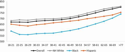
Figure B2. Median balance in any debt by age cohort, 2016

Note: Authors' calculations using anonymized credit bureau data from 2016.

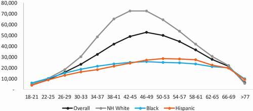
Figure B3. Student debt

Panel A. Percentage of consumers with student loan debt by age cohort, 2016.

Panel B. Median student loan balance (in dollars) in the population with student loan debt, 2016. Note: Authors' calculations using anonymized credit bureau data from 2016.

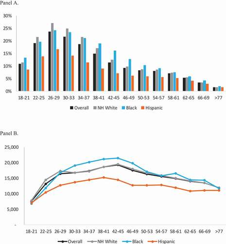
Figure B4. Credit card debt

Panel A. Percentage of consumers with some credit card debt by age cohort, 2016.Panel B. Median credit card debt balance (in dollars) in the population with credit card debt, 2016. Note: Authors' calculations using anonymized credit bureau data from 2016.

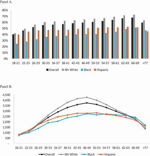
Figure B5. Auto debt

Panel A. Percentage of consumers with some auto debt by age cohort, 2016. Panel B. Median auto loan debt balance (in dollars) in the population with auto loan debt, 2016. Note: Authors' calculations using anonymized credit bureau data from 2016.

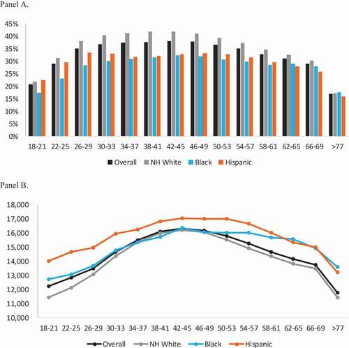
Figure B6. Population share with any foreclosures in the past 84 months (since September 2016) by age cohort

Note: Authors' calculations using anonymized credit bureau data from 2016.

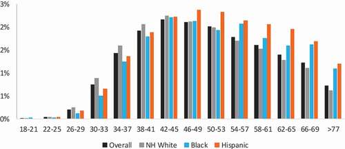
Figure B7. Population share with any bankruptcies in the past 84 months (since September 2016) by age cohort

Note: Authors' calculations using anonymized credit bureau data from 2016.

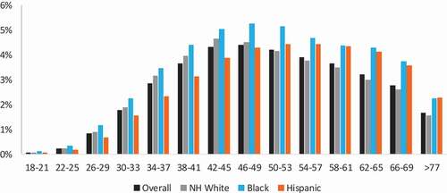
Figure B8. Population share with thin files and with clean credit records by age cohort, 2016

Consumers with thin files with clean credit records are defined as those with few trade lines (two or fewer) reported in their credit records and no delinquencies in the last 180 days, no foreclosures in the last 84 months, and no bankruptcies in the last 84 months, and whose back-end debt-to-income (DTI) ratio does not exceed 25. NOTE: Authors' calculations using anonymized credit bureau data from 2016.

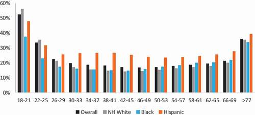
Appendix C.

Racial/Ethnic Mortgage Ownership Patterns, 2012–2018.

Our credit bureau data capture the total number of open mortgage-type trade lines reported in the previous 6 months for all 3 years. This field allows us to track mortgage ownership status over time. Panel A in Table C1 shows the 2018 mortgage ownership status by the 2012 mortgage ownership status for the overall, non-Hispanic White, Black, and Hispanic populations, respectively. Whereas 61.3% of the overall population did not have a mortgage in either year, 21.9% of them had mortgages in both years. Another 8.31% of borrowers had a mortgage in 2012 but were no longer mortgage owners by 2018. Most importantly, 8.40% of the overall population did not have a mortgage in 2012 and transitioned into mortgage ownership by 2018. These percentages are 8.99% for non-Hispanic Whites, 5.16% for Blacks, and 7.43% for Hispanics. In Table C2, we investigate whether these estimated racial differences in rates of transition to new mortgages are statistically meaningful. Both the pooled (equal variance) and Satterthwaite (unequal variance) test results indicate that White–Black and White–Hispanic gaps in transition rates are highly statistically significant.

In panel B of Table C1, we define the rate of transition to mortgage ownership as the percentage of 2012 nonmortgage owners who obtained a new mortgage by 2018. Overall, the rate of transition to mortgage ownership is around 12%. Black and Hispanic consumers transitioned into mortgage ownership at a much lower rate than non-Hispanic White consumers (6.3%, Black; 9.5%, Hispanic; 13.8%, White). The estimates indicate that Blacks and Hispanics are approximately one half and two thirds as likely to enter into mortgage ownership as Whites, respectively. Furthermore, Table C3 reports the rate of transition to new mortgages from 2012 to 2016 by race/ethnicity and indicates that the racial/ethnic transition rate gap is widening over time.

Panel C of Table C1 reports the percentage of 2012 mortgage owners who transitioned out of mortgage ownership by 2018. Since the estimated share of individuals who transitioned out of a mortgage likely includes both (a) those who paid off their mortgage and (b) those who lost their home to foreclosure, we separate the estimated share of who transitioned out by those with observed foreclosure and those without observed foreclosure between 2011 and 2018. As Table C1 suggests, most 2012 mortgage holders who transitioned out by 2018 did not have any observed foreclosure in the prior 7 years (around 26%). Overall, only 1.4% of 2012 mortgage holders who transitioned out of mortgages by 2018 had an observed foreclosure in the prior 7 years. This percentage is slightly higher for minorities compared with non-Hispanic Whites (Blacks: 2.9%; Hispanics: 1.9%; non-Hispanic Whites: 1.3%).

There could be several reasons for exiting mortgage ownership, such as short sales, severe delinquencies leading to foreclosure of the property, or paying off the mortgage debt. Unfortunately, our data do not allow us to disentangle these possibilities because we cannot observe the tenure status of consumers, origination date, or origination loan amount.³⁷ In Table C4, we look into the age distribution of this population and find that consumers who transitioned out of mortgage ownership are more likely to be older. In particular, they are more likely to be age 66+, and hence are more likely to own their home free and clear.

Table C1. Mortgage ownership rate by year and mortgage transition rates, 2012–2018

Panel A: 2018 Mortgage Ownership Status
	Overall		Non-Hispanic White		Black		Hispanic
	N = 4,539,574		N = 3,009,849		N = 513,398		N = 672,294
	NoMortgage	Has amortgage	NoMortgage	Has amortgage	NoMortgage	Has amortgage	NoMortgage	Has amortgage
No mortgage in 2012	61.34%	8.40%	56.38%	8.99%	76.52%	5.16%	71.17%	7.43%
Had a mortgage in 2012	8.31%	21.95%	9.45%	25.17%	5.46%	12.85%	5.87%	15.52%
Panel B: Transition Into Mortgage Ownership (2012-2018)
	Overall		Non-Hispanic White		Black		Hispanic
	N=3,165,899		N=1,967,538		N=419,343		N=528,423
Percent of 2012 non-mortgage holders who are new mortgage holders in 2018	12.05%		13.75%		6.32%		9.46%
Panel C: Transition Out of Mortgage Ownership (2012-2018)
	Overall		Non-Hispanic White		Black		Hispanic
	N = 1,373,675		N = 1,042,010		N = 94,003		N = 143,804
Percent of 2012 Mortgage holders who are non-mortgage holders in 2018 (with observed foreclosure)	1.43%		1.27%		2.85%		1.92%
Percent of 2012 Mortgage holders who are non-mortgage holders in 2018 (without observed foreclosure)	26.03%		26.04%		26.97%		25.54%

Table C2. Results from t-test on White–Black and White–Hispanic gaps in rates of transition to new mortgages from 2012 to 2018

Variable: Race	N	Mean	SD	SE	Min	Max
NH White	30,09,849	0.0899	0.2860	0.0002	0	1
Black	5,13,398	0.0516	0.2212	0.0003	0	1
Difference (NH White- Black)		0.0383	0.2775	0.0004
Variable: Race	Method	Mean		95% CL Mean	SD		95% CL SD
NH White		0.0899	0.0896	0.0902	0.286	0.2858	0.2863
Black		0.0516	0.051	0.0522	0.2212	0.2208	0.2216
Difference (NH White- Black)	Pooled	0.0383	0.0375	0.0391	0.2775	0.2773	0.2777
Difference (NH White- Black)	Satterthwaite	0.0383	0.0376	0.039
Method	Variances	DF	t Value	Pr > |t|
Pooled	Equal	35,20,000	91.41	<.0001
Satterthwaite	Unequal	8,36,428	109.45	<.0001
Equality of Variances
Method	Num DF	Den DF	F Value	Pr > F
Folded F	30,10,000	5,13,397	1.67	<.0001
Variable: Race	N	Mean	SD	SE	Min	Max
NH White	30,09,849	0.0899	0.2860	0.0002	0	1
Hispanic	6,72,294	0.0743	0.2623	0.0003	0	1
Difference (NH White- Hispanic)		0.0155	0.2818	0.0004
Variable: Race	Method	Mean		95% CL Mean	SD		95% CL SD
NH White		0.0899	0.0896	0.0902	0.286	0.2858	0.2863
Black		0.0743	0.0737	0.075	0.2623	0.2619	0.2628
Difference (NH White- Hispanic)	Pooled	0.0155	0.0148	0.0163	0.2818	0.2816	0.2821
Difference (NH White- Hispanic)	Satterthwaite	0.0155	0.0148	0.0162
Method	Variances	DF	t Value	Pr > |t|
Pooled	Equal	36,80,000	40.88	<.0001
Satterthwaite	Unequal	10,60,000	43.18	<.0001
Equality of Variances
Method	Num DF	Den DF	F Value	Pr > F
Folded F	3.01E+06	672293	1.19	<.0001

Note. NH = Non-Hispanic. SD = standard deviation. SE = standard error.

Table C3. Mortgage ownership rates by year and rates of transition to mortgage ownership, 2012–2016

Panel A: 2016 Mortgage Ownership Status
	Overall		Non-Hispanic White		Black/African American		Hispanic
	N = 4,539,574		N = 3,009,849		N = 513,398		N = 672,294
	No Mortgage	Has a mortgage	No Mortgage	Has a mortgage	No Mortgage	Has a mortgage	No Mortgage	Has a mortgage
No mortgage in 2012	63.55%	6.19%	58.64%	6.74%	78.03%	3.65%	73.41%	5.19%
Had a mortgage in 2012	6.21%	24.05%	7.04%	27.59%	4.15%	14.16%	4.50%	16.89%
Panel B: Transition Into Mortgage Ownership (2012-2016)
New Mortgage Holders as a percent of 2012 Non-Mortgage Holders	Overall		Non-Hispanic White		Black/African American		Hispanic
	8.88%		10.25%		4.49%		6.63%

The rate of transition to mortgage ownership gives the share of nonmortgage holders in 2012 who entered mortgage ownership in 2016.

Table C4. Age distribution of mortgage holders, 2012

Variable	Category	Mortgage Holders in 2012	Transition out of mortgages by 2018	Did not transition out of mortgages by 2018
		N = 1,373,637	N = 377,217	N = 996,420
Age cohort (2018)	Missing	0.0044	0.0091	0.0026
Age cohort (2018)	18 ≤ age ≤25	0.0003	0.0003	0.0003
Age cohort (2018)	26 ≤ age ≤ 35	0.0458	0.0408	0.0477
Age cohort (2018)	36 ≤ age ≤ 45	0.1707	0.1345	0.1844
Age cohort (2018)	46 ≤ age ≤ 55	0.2528	0.2048	0.2709
Age cohort (2018)	56 ≤ age ≤ 65	0.2711	0.2717	0.2709
Age cohort (2018)	66 ≤ age ≤ 70	0.1051	0.1233	0.0981
Age cohort (2018)	Above 70	0.1498	0.2154	0.1250
Mean Age (2018)		56.6317	59.5024	55.5519

Appendix D.

Sources of Down Payment by Race/Ethnicity

In this Appendix, we report the different sources of down payment used by mortgage borrowers based on the National Survey of Mortgage Originations (NSMO). The survey is jointly funded and managed by the Federal Housing Finance Agency (FHFA) and Consumer Financial Protection Bureau (CFPB) and is a component of the National Mortgage Database (NMDB).³⁸ The NSMO is a nationally representative, quarterly survey of new mortgage loans. The survey asks borrowers about the source of the down payment on their recent purchase of a home. For our analysis, we use the NSMO survey data for mortgages originated from 2013 through 2017.

Table D1 gives the percentage of White and Black respondents who used the listed sources for their down payments. As the table suggests, Blacks rely more than Whites on savings, inheritance, gifts, and grants from family or friends to meet their down payment requirements. On the other hand, compared with Whites, Blacks rely less on proceeds from the sale of another property.

Table D1. Percentages of the White and Black respondents using different sources for the down payment

Year	Race	Savings, retirement account, inheritance, or other assets	Proceeds from sale of another property	Assistance or loan from a nonprofit or government agency	A sceond lien, home equity loan, or home equity line of credit	Gift or loan from family or friend	Seller contribution
2013	White	79%	23%	5%	0%	20%	16%
	Black	82%	7%	12%	0%	27%	24%
2014	White	75%	27%	6%	0%	23%	15%
	Black	82%	7%	18%	0%	18%	27%
2015	White	73%	29%	6%	4%	21%	17%
	Black	81%	10%	16%	5%	23%	28%
2016	White	70%	31%	7%	3%	21%	15%
	Black	75%	15%	19%	4%	24%	30%
2017	White	70%	30%	8%	3%	21%	18%
	Black	77%	17%	16%	1%	23%	36%

The percentages do not add up to 100% as the respondents chose more than one option in some instances.

Appendix E.

Robustness Check

We perform several robustness checks on our results. All the specifications discussed below are computed at pooled coefficients. For each specification, we compare the model fit, marginal probabilities, and results from the decomposition exercise with our baseline specification.

Age: Around 5% of our estimation sample is missing age data. Since age is an important determinant of mortgage borrowing, we test the implications of this data limitation. We run an alternative specification by dropping all consumers with missing age (see Table E1, column heading Excluding missing age). Table E1 shows that our regression results remain unchanged and estimated coefficients are similar to the baseline case for almost all variables. Table E2 gives the results from the decomposition exercise, which reveal that most of the baseline results hold. In particular, credit profile explains most of the racial/ethnic gap in the transition rate, followed by severe derogatory credit. Whereas geography consistently matters more in explaining the White–Hispanic gap, household composition explains more of the White–Black gap.

Next, one could argue that some individuals in our estimation sample who did not transition to mortgage ownership between 2012 and 2018 might own their house free and clear. These homeowners are likely to be older and have more established credit profiles compared with the renters. Further, older borrowers who own their house free and clear may acquire a new mortgage for reasons other than purchasing a home, such as paying for the education of a child or healthcare bills, which is difficult for us to disentangle. Recognizing this, we focus on the population that is more likely to be representative of new mortgage owners who have not yet paid off their mortgage debt as a robustness check (see Table E2, column headed Age ≤55). To this end, we purge the older consumers by restricting the individuals in our sample to those 55 and younger. This population is more likely to be representative of first-time homebuyers who have not yet paid off their mortgage debt.³⁹ As Tables E1 and E2 suggest, our results are largely robust, with a few differences. First, the racial/ethnic difference in age distribution plays a lesser role in explaining the White–minority gap in the transition rate. Second, the contribution of credit profile also declines (35% to 38%), compared with the baseline specification, as the racial/ethnic difference in credit scores declines when the population is skewed younger. Lastly, income growth positively contributes to the White–Hispanic gap because Hispanic income grew at a lower rate than that of Whites for this population.

Credit scores: In our benchmark specification, we have four transition missing FICO indicators. One could argue that the indicator for individuals who had a missing FICO score in 2012 but an observed FICO score by 2018 may be endogenous to mortgage receipt. To address this, we ran a robustness check in which we consider a single indicator of whether FICO is missing in 2012 (see Tables E1 and E2, column headed No missing transition FICO indicators). Both the likelihood ratio test and pseudo R² reported in Table E1 suggest a lower fit compared with our baseline case. Moreover, the regression results indicate that, compared with consumers with a FICO score in 2012, consumers who had a missing FICO score in 2012 are more likely to transition to new mortgages by 2018, which is counterintuitive.⁴⁰ Despite this, Table E2 indicates that credit profile consistently explains most of the White–minority gap in this specification. By using the transition variables in our baseline specification, we are able look more closely at the group with a missing FICO score in 2012 to understand why they appear more likely to obtain a new mortgage. These individuals could be those taking steps to move into homeownership or increasing their demand for credit in general, which could put them in a better position to obtain a mortgage.

Next, FICO score can have a nonlinear relationship with the propensity to own a mortgage. To investigate, we run an alternative specification with FICO buckets instead of a continuous FICO score (see Table E1, column headed FICO buckets). Under this specification, consumers’ FICO score in 2012 is transformed into four categories: missing, less than 620, 620–700, and more than 700. We use the last category as the reference category. The marginal probabilities under this specification, as given in Table E1, do not suggest a nonlinear relationship between FICO and transition probability. For example, compared with consumers who had FICO scores of more than 700, consumers with lower FICO scores (less than 620, 620–700) have monotonically lower transition probabilities to mortgage ownership. Furthermore, whereas the goodness-of-fit tests indicate a lower fit of this specification compared with the baseline case, our decomposition exercise in Table E2 reveals our baseline results are robust to this alternative specification.

An important component of the credit profile that primarily contributes to the White–minority gap is the FICO score. In our benchmark case, we use the FICO score as a measure of credit risk because it was the most common industry practice at the time of the study. How sensitive are our results to alternative credit scoring models? Our credit bureau data include borrower-level information on VantageScore 3.0 (see Table E1, column headed Vantage score), which allows us to carry this sensitivity test. Table E3 presents the average Vantage score, the percentage with a missing Vantage score, and the adjusted Vantage score in 2012. Less than 0.5% of our sample had a missing Vantage score in 2012, suggesting that the Vantage score has much better coverage compared with the FICO score. Because the percentage of missing Vantage scores is so low, adjusted Vantage scores are very similar to unadjusted ones. Moreover, both minority groups have a lower average adjusted Vantage score compared with non-Hispanic Whites (Whites: 662.85; Blacks: 582.92; Hispanics: 618.87). The results from the decomposition exercise in Table E2 suggest that when the Vantage score is used instead of the FICO score, the racial/ethnic differences in credit profiles continue to dominate all factors in contributing to the White–minority gap, hence reinforcing our baseline results.

Severe derogatory credit: In our baseline model specification, we included indicators of any foreclosures and bankruptcies in the 84 months prior to September 2018. One could argue that because foreclosure and bankruptcy may lead to homeownership exit, including 2018 values of these variables may be endogenous to mortgage transition by 2018. To this end, we run an alternative specification that includes 2012 values of these variables. Table E4 gives the marginal probabilities under this specification (column headed Foreclosure and bankruptcies in 2012) and indicates that compared with consumers with no bankruptcies, consumers who have experienced bankruptcies (recent and old) are more likely to transition to mortgage ownership, which is counterintuitive. Furthermore, the results from the decomposition exercise reveals that severe derogatory credit explains 12% of the White–minority gap under this specification, which is similar to the baseline specification (see Table E5).

Next, credit scores are likely to be highly correlated with delinquencies, which may cause instability in the model. The proprietary nature of credit scoring models makes it impossible to know the extent to which delinquencies impact credit scores. To investigate, we run an alternative specification, dropping the 90-day delinquency indicator. Table E4 indicates marginal probabilities for credit scores under this alternative specification (see the column headed Excluding 90-day delinquency indicator) are almost unchanged compared with baseline specification. Moreover, the model fit is slightly worse than the baseline specification. Whereas credit scores and delinquencies may be highly correlated, other factors in the credit scoring model matter as well. Hence, any potential degree of correlation with delinquency does not affect the overall predictiveness of the model.

Income and debt-to-income ratio: Next, in our baseline model specification, we used the estimated tax-reported income included in our credit bureau data to construct income growth. As a robustness check, we ran a version of our model by substituting estimated tax-reported income with income data at the census-tract level. Using 5-year estimates from 2012 and 2018 from the ACS, we computed income growth rate at the census-tract level. Table E5, which gives the decomposition results under this specification (see the column headed Census tract income), suggests our results are robust to alternative measures of income. Whereas credit profile is still a dominant source of the White–minority gap, income growth plays a less important role.

A few independent variables, such as income and DTIs, enter in our benchmark specification as growth rates. However, it is possible that the changes in these variables are endogenous to the change in tenure status. For example, consumers with higher income growth from 2012 to 2018 are more likely to own a house. To address the possible endogeneity, we run a version of our model with 2012 values of income and DTI levels (see Table E5, column headed Level values (income, DTI)). The decomposition results in Table E5 suggest that the income level in 2012 explains around 21–35% of the White–minority gap. This is mainly because in 2012 Whites had a higher average income compared with both minority groups under this specification (White: $79,115; Black: $55,383; Hispanic: $60,278). Furthermore, DTI levels in 2012 are less predictive of the probability of transitioning to mortgage by 2018 (see Table E4), especially for consumers who transitioned closer to 2018. Hence, the contribution of the credit profile category, which includes DTIs, to explaining the White–minority gap declined slightly, from 45–68% in the benchmark case to 40–56% in this case. Despite this, credit profile continues to be a dominant factor in explaining the gap.

Mortgage inquiry: As mentioned, an important factor that contributes to a consumer’s decision to transition to homeownership is mortgage demand. Estimation of the effect of mortgage inquiries on homeownership is complicated by the presence of other factors that influence both mortgage demand and homeownership decisions. For example, consumers preparing for homeownership in the near future might inquire more about mortgages and also might be more likely to own a home in future. We check the sensitivity of our results by excluding mortgage inquiries from our baseline model with pooled racial/ethnic groups (see Table E5, colomn headed Excluding mortgage inquiries). Table E4 shows that our regression results remain unchanged and estimated coefficients are similar to the baseline case for almost all the variables. Table E5 presents the results from the decomposition exercise under this specification. Most of the baseline results hold. In particular, credit profile explains most of the racial/ethnic gap in the transition rate, followed by severe derogatory credit. Whereas geography consistently matters more in explaining the White–Hispanic gap, household composition explains more of the White–Black gap.

Affordability index: Although it is at a historic low, geographic mobility may affect an individual’s propensity to apply for new mortgages. For example, young individuals moving to New York or San Francisco face different housing affordability constraints than do young individuals moving to Nashville or Dallas. Even though investigating the relationship between geographic mobility and homeownership falls out of the scope of this article, we run an alternative specification by controlling for affordability index ex post obtaining new mortgages. In particular, we include house price-to-income ratio in 2018 instead of 2012, as a proxy for migration (see Tables E4 and E5, colum headed Affordability index, 2018). Our results from both the regression exercise (see Table E4) and the decomposition exercise (see Table E5) suggest that all our baseline results hold under this specification.

Table E1. Logit models of transition to mortgage ownership under alternative specifications (age, credit score)

Variable	Category	Baseline Model (Pooled coefficients)	Excluding missing age	Age ≤ 55	No missing transition FICO indicators	FICO buckets	Vantage score
Gender	Female	-0.0213***	-0.0223***	-0.0268***	-0.019***	-0.0187***	-0.0186***
		(-52.97)	(-52.69)	(-47.41)	(-47.2)	(-46.44)	(-46.3)
Gender	Indefinite/Uncertain	-0.049***	-0.0534***	-0.0679***	-0.052***	-0.0521***	-0.0519***
		(-6.59)	(-6.8)	(-6.83)	(-7.32)	(-7.38)	(-7.34)
Gender	Unknown	-0.0392***	-0.0412***	-0.0475***	-0.0406***	-0.0411***	-0.0406***
		(-46.7)	(-46.37)	(-42.94)	(-49.45)	(-50.31)	(-49.84)
Age cohort	Missing	-0.0266***	-	-	-0.0333***	-0.04***	-0.0347***
		(-29.92)	-	-	(-55.04)	(-67.03)	(-67.86)
Age cohort	18 ≤ age ≤25	0.0308***	0.0318***	-	0.0423***	0.0269***	0.0474***
		(26.95)	(26.83)	-	(34)	(23.35)	(37.35)
Age cohort	26 ≤ age ≤ 35	0.0993***	0.1034***	0.0677***	0.1078***	0.096***	0.1157***
		(167.7)	(167.76)	(57)	(179.93)	(160.45)	(190.09)
Age cohort	36 ≤ age ≤ 45	0.1265***	0.1317***	0.0983***	0.1322***	0.1226***	0.1368***
		(187.64)	(188.07)	(76.43)	(193.92)	(178.8)	(199.71)
Age cohort	46 ≤ age ≤ 55	0.1111***	0.1157***	0.0794***	0.1146***	0.107***	0.1168***
		(162.45)	(162.79)	(60.19)	(166.78)	(153.48)	(170.47)
Age cohort	56 ≤ age ≤ 65	0.0777***	0.0809***	-	0.08***	0.0768***	0.0803***
		(123.37)	(123.55)	-	(127.38)	(117.8)	(129.39)
Age cohort	66 ≤ age ≤ 70	0.0476***	0.0496***	-	0.0495***	0.0497***	0.049***
		(61.27)	(61.34)	-	(63.86)	(60.74)	(64.44)
Number of children (2018)		-0.0015***	-0.0016***	-0.0031***	-0.0012***	-0.0012***	-0.0011***
		(-6.09)	(-6.35)	(-9.86)	(-4.8)	(-4.81)	(-4.55)
Marital status (2012)	Single	-0.0628***	-0.0664***	-0.0824***	-0.066***	-0.0672***	-0.0632***
		(-96.38)	(-96.52)	(-89.68)	(-101.66)	(-104.01)	(-97)
Marital status (2012)	Unknown	-0.0201***	-0.0214***	-0.0303***	-0.0211***	-0.0223***	-0.0195***
		(-43.24)	(-43.69)	(-44.96)	(-44.75)	(-47.5)	(-41.74)
Marital status transition	2012=single; 2018=married	0.0789***	0.0832***	0.0989***	0.0811***	0.0816***	0.0796***
		(79.66)	(79.57)	(76.14)	(81.75)	(82.25)	(80.34)
Marital status transition	2012=married; 2018=single	-0.0651***	-0.0688***	-0.0861***	-0.0661***	-0.0676***	-0.0636***
		(-65.51)	(-65.63)	(-65.73)	(-66.17)	(-67.69)	(-63.93)
Income (growth rate)		0.1305***	0.1374***	0.1651***	0.1398***	0.1383***	0.1448***
		(284.67)	(283.92)	(270.28)	(299.01)	(295.23)	(312.5)
Education level (2018)	HS diploma	-0.0175***	-0.0185***	-0.0227***	-0.0166***	-0.016***	-0.0164***
		(-26.24)	(-26.19)	(-23.92)	(-25.1)	(-24.27)	(-24.75)
Education level (2018)	Some College	0.0089***	0.0094***	0.0091***	0.0116***	0.0122***	0.0116***
		(13.19)	(13.29)	(9.85)	(17.3)	(18.22)	(17.37)
Education level (2018)	Bachelors degree	0.0117***	0.0125***	0.0093***	0.0145***	0.0164***	0.013***
		(15.91)	(16)	(9.22)	(19.63)	(22.25)	(17.7)
Education level (2018)	Graduate degree	0.0139***	0.0149***	0.0127***	0.0161***	0.0188***	0.0138***
		(16.66)	(16.87)	(11.05)	(19.17)	(22.39)	(16.56)
Education level (2018)	Unknown	-0.0222***	-0.0234***	-0.0345***	-0.0269***	-0.026***	-0.0277***
		(-9.68)	(-9.65)	(-8.64)	(-12.46)	(-12.09)	(-12.95)
Adjusted FICO score (2012)		0.0003***	0.0004***	0.0006***	0.0004***	-	-
		(116.54)	(116.5)	(148.52)	(132.24)	-	-
Missing FICO indicator	2012=missing, 2018=not missing	0.202***	0.2126***	0.3563***	-	-	-
		(100.28)	(99.98)	(127.4)	-	-	-
Missing FICO indicator	2012=not missing, 2018=missing	-0.6517***	-0.6854***	-0.7683***	-	-	-
		(-22.34)	(-22.28)	(-18.12)	-	-	-
Missing FICO indicator	2012=missing, 2018=missing	-0.3468***	-0.3633***	-0.3305***	-	-	-
		(-20.45)	(-20.31)	(-11.42)	-	-	-
Missing FICO indicator	2012=missing	-	-	-	0.1936***	-	-
		-	-	-	(96.84)	-	-
FICO bucket	Less than 620	-	-	-	-	-0.098***	-
		-	-	-	-	(-135.72)	-
FICO bucket	620 ≤ FICO <700	-	-	-	-	-0.0247***	-
		-	-	-	-	(-37.19)	-
FICO bucket	Missing	-	-	-	-	-0.1019***	-
		-	-	-	-	(-133.51)	-
Vantage score (2012)		-	-	-	-	-	0.0005***
		-	-	-	-	-	(171.81)
Missing Vantage indicator	2012=missing	-	-	-		-	0.213***
		-	-	-		-	(36.56)
Thin file indicator (2012)		-0.035***	-0.036***	-0.0413***	-0.0414***	-0.0462***	-0.0442***
		(-66.01)	(-64.32)	(-56.68)	(-77.82)	(-87.65)	(-84.7)
Household DTI growth	Student Debt	-0.0131***	-0.0138***	-0.0155***	-0.0127***	-0.0122***	-0.0126***
		(-36.59)	(-36.62)	(-34.91)	(-35.35)	(-33.8)	(-34.75)
Household DTI growth	Auto Debt	0.0092***	0.0097***	0.0141***	0.014***	0.0153***	0.0126***
		(18.83)	(18.84)	(22.23)	(27.56)	(30.06)	(25)
Household DTI growth	Credit Card	0.049***	0.0513***	0.0652***	0.0526***	0.058***	0.0475***
		(53.49)	(53.11)	(54.46)	(55.75)	(60.89)	(50.94)
All 90D indicator (2012)		-0.0282***	-0.0297***	-0.0268***	-0.0338***	-0.0328***	-0.0237***
		(-44.04)	(-44)	(-30.71)	(-52.1)	(-51.55)	(-37.36)
Foreclosure in 84 months indicator (2018)		0.0249***	0.026***	0.0163***	0.0286***	0.0263***	0.031***
		(7.12)	(7.04)	(3.31)	(8.19)	(7.49)	(8.89)
Bankruptcy (2018)	0< bankruptcy <12 (months ago)	-0.0875***	-0.0923***	-0.1119***	-0.0862***	-0.0875***	-0.0842***
		(-40.36)	(-40.28)	(-35.64)	(-38.88)	(-40.52)	(-36.77)
Bankruptcy (2018)	12≤ bankruptcy <24 (months ago)	-0.086***	-0.0907***	-0.1067***	-0.0883***	-0.0895***	-0.0863***
		(-38.3)	(-38.22)	(-32.18)	(-41.76)	(-43.27)	(-39.36)
Bankruptcy (2018)	24≤ bankruptcy <36 (months ago)	-0.0828***	-0.0873***	-0.1055***	-0.0839***	-0.0856***	-0.0816***
		(-33.12)	(-33.05)	(-29.2)	(-34.51)	(-36.33)	(-32.35)
Bankruptcy (2018)	36≤ bankruptcy <48 (months ago)	-0.0552***	-0.0583***	-0.0652***	-0.0553***	-0.0575***	-0.0522***
		(-17.89)	(-17.91)	(-14.52)	(-18.06)	(-19.24)	(-16.52)
Bankruptcy (2018)	48≤ bankruptcy <60 (months ago)	-0.0092***	-0.0096***	-0.0103**	-0.0072**	-0.0124***	-0.0032
		(-2.64)	(-2.61)	(-2.07)	(-2.04)	(-3.62)	(-0.88)
Bankruptcy (2018)	60≤ bankruptcy <72 (months ago)	0.0349***	0.0369***	0.0422***	0.0402***	0.035***	0.0442***
		(8.25)	(8.28)	(7.13)	(9.21)	(8.2)	(9.99)
Bankruptcy (2018)	≥72 (months ago)	0.1019***	0.1075***	0.0982***	0.1128***	0.1209***	0.0962***
		(25.57)	(25.61)	(18)	(26.87)	(28.2)	(23.93)
Mortgage inquiry indicator (2012)		0.1245***	0.131***	0.1306***	0.1298***	0.1284***	0.13***
		(243.84)	(243.3)	(182.24)	(251.16)	(248.61)	(252.01)
Unemployment rate (2012)		-0.415***	-0.4386***	-0.5705***	-0.4215***	-0.4422***	-0.4078***
		(-29.75)	(-29.77)	(-28.54)	(-30.11)	(-31.6)	(-29.25)
House price-to -income ratio (2012)	Single Family, median value and logged	-0.0576***	-0.0609***	-0.0859***	-0.0577***	-0.0579***	-0.0598***
		(-67.92)	(-67.91)	(-71.68)	(-67.62)	(-67.94)	(-70.24)
State dummies		yes	yes	yes	yes	yes	yes
-2Log L		1371811.58	1366154.2	9,54,072.02	14,17,050.82	14,15,252.70	14,09,755.34
chi2		464350.02	430876.16	3,32,592.33	4,19,110.79	4,20,908.90	4,26,406.26
Pseudo R squared		0.2529	0.2398	0.2585	0.2283	0.2292	0.2322
Number of observations used		23,94,597	22,64,541	14,39,986	23,94,597	23,94,597	23,94,597

Note. All 90D = an indicator for 90-day delinquencies in 2012. DTI = debt to income ratio. FICO = Fair Isaac Corporation. Indefinite/uncertain gender = name could be either male or female.

The dependent variable is the binary indicator of mortgage transition by 2018 for a sample of nonmortgage holders in 2012. The reported coefficients are the marginal probability with respect to explanatory variables. t statistics are reported in parentheses. Likelihood ratio test results, which evaluate the goodness of fit in the case of incremental inclusion, are reported.

*p < .05. **p < .01. ***p < .001.

Table E2. Decomposition results under alternative specifications (age, credit score)

Panel A. Decomposition of difference between Black and Non-Hispanic (NH) White transition rates into mortgage ownership
Mean Values of Decomposition Runs (NH White-Black gap)	Baseline Model (Pooled coefficients)	Excluding missing age	Age ≤ 55	No missing transition FICO indicators	FICO buckets	Vantage score
NH White transition rate	0.1453	0.1532	0.1789	0.1453	0.1453	0.1453
Black transition rate	0.0662	0.0684	0.0697	0.0662	0.0662	0.0662
NH White-Black gap	0.0791	0.0847	0.1091	0.0791	0.0791	0.0791
Contributions from racial differences in:
Individual demographics	-0.017	-0.017	-0.004	-0.021	-0.018	-0.023
	0.000	0.000	0.000	0.000	0.000	0.000
	-21%	-20%	-3%	-27%	-22%	-29%
Household composition	0.009	0.010	0.007	0.010	0.009	0.010
	0.000	0.000	0.000	0.000	0.000	0.000
	11%	11%	7%	12%	12%	12%
Income growth	0.005	0.005	0.010	0.004	0.004	0.003
	0.000	0.000	0.000	0.000	0.000	0.000
	6%	6%	9%	5%	5%	4%
Education	0.002	0.002	0.002	0.002	0.002	0.002
	0.000	0.000	0.000	0.000	0.000	0.000
	2%	2%	2%	3%	3%	2%
Credit profiles	0.035	0.038	0.042	0.037	0.033	0.046
	0.000	0.000	0.000	0.000	0.000	0.000
	45%	44%	38%	47%	42%	58%
Severe derogatory credit	0.007	0.008	0.006	0.009	0.008	0.006
	0.000	0.000	0.000	0.000	0.000	0.000
	9%	9%	5%	11%	11%	7%
Mortgage inquiry	0.009	0.009	0.009	0.009	0.009	0.009
	0.000	0.000	0.000	0.000	0.000	0.000
	11%	11%	9%	12%	12%	12%
Geography	0.002	0.003	0.003	0.002	0.002	0.002
	0.000	0.000	0.000	0.000	0.000	0.000
	3%	3%	3%	3%	3%	3%
Percentage explained by all variables included	66%	67%	70%	65%	65%	69%
Mean Values of Decomposition Runs (NH White-Hispanic gap)	Baseline Model (Pooled coefficients)	Excluding missing age	Age ≤ 55	No missing transition FICO indicators	FICO buckets	Vantage score
Panel B. Decomposition of difference between Hispanic and Non-Hispanic (NH) White transition rates into mortgage ownership
NH White transition rate	0.1453	0.1532	0.1789	0.1453	0.1453	0.1453
Hispanic transition rate	0.1056	0.1116	0.1156	0.1056	0.1056	0.1056
NH White-Hispanic gap	0.0398	0.0416	0.0633	0.0398	0.0398	0.0398
Contributions from racial differences in:
Individual demographics	-0.024	-0.025	-0.007	-0.027	-0.024	-0.029
	0.000	0.000	0.000	0.000	0.000	0.000
	-61%	-60%	-11%	-69%	-59%	-73%
Household composition	0.002	0.003	0.000	0.002	0.002	0.003
	0.000	0.000	0.000	0.000	0.000	0.000
	6%	6%	0%	6%	5%	6%
Income growth	-0.003	-0.004	0.005	-0.005	-0.004	-0.006
	0.000	0.000	0.000	0.000	0.000	0.000
	-7%	-8%	7%	-12%	-11%	-15%
Education	0.003	0.003	0.004	0.004	0.004	0.003
	0.000	0.000	0.000	0.000	0.000	0.000
	8%	8%	6%	9%	10%	8%
Credit profiles	0.027	0.028	0.022	0.031	0.025	0.035
	0.000	0.000	0.000	0.000	0.000	0.000
	68%	68%	35%	78%	62%	88%
Severe derogatory credit	0.004	0.004	0.002	0.005	0.004	0.003
	0.000	0.000	0.000	0.000	0.000	0.000
	10%	10%	4%	12%	11%	7%
Mortgage inquiry	0.003	0.003	0.004	0.003	0.003	0.003
	0.000	0.000	0.000	0.000	0.000	0.000
	6%	6%	6%	8%	8%	8%
Geography	0.019	0.020	0.024	0.019	0.019	0.019
	0.000	0.000	0.000	0.000	0.000	0.000
	48%	49%	38%	47%	48%	49%
Percentage explained by all variables included	79%	78%	85%	79%	75%	79%

Note. Each row gives the coefficient, standard errors (in parentheses) and percentage contribution by each category of variables to the racial/ethnic difference in transition gap.

Table E3. Average Vantage 3.0 score and percentage of missing Vantage scores for the estimation sample

	Full estimation sample	Transitioned to mortgage by 2018	Did not transition to mortgage by 2018
	N = 2,347,247	N = 301,156	N = 2,046,091
Mean Vantage (2012)	648.77	688.92	642.84
Missing Vantage (%)	0.34	0.09	0.37
Mean adjusted Vantage (2012)	646.58	688.30	640.44

Table E4. Logit models of transition to mortgage ownership under alternative specifications (severe derogatory credit, income, debt-to-income ratio [DTI], mortgage inquiry, affordability index)

Variable	Category	Baseline Model (Pooled coefficients)	Foreclosure and Bankruptcies in 2012	Excluding 90 days delinquency indicator	Census tract income	Level values (income, DTI)	Excluding mortgage inquiries	Affordability index, 2018
Gender	Female	-0.0213***	-0.0208***	-0.0212***	-0.0233***	-0.0227***	-0.0238***	-0.0211***
		(-52.97)	(-52.2)	(-52.83)	(-55.32)	(-55.45)	(-57.96)	(-51.85)
Gender	Indefinite/Uncertain	-0.049***	-0.0482***	-0.0491***	-0.0506***	-0.0476***	-0.0525***	-0.048***
		(-6.59)	(-6.45)	(-6.58)	(-6.44)	(-6.14)	(-6.97)	(-6.35)
Gender	Unknown	-0.0392***	-0.0375***	-0.0391***	-0.0386***	-0.0362***	-0.0433***	-0.0392***
		(-46.7)	(-44.41)	(-46.46)	(-43.29)	(-41.28)	(-50.95)	(-46.14)
Age cohort	Missing	-0.0266***	-0.0264***	-0.026***	-0.0188***	-0.0188***	-0.0243***	-0.0271***
		(-29.92)	(-29.07)	(-29.37)	(-25.39)	(-28.57)	(-31.05)	(-30.17)
Age cohort	18 ≤ age ≤25	0.0308***	0.0328***	0.0337***	0.0724***	0.0806***	0.0295***	0.0307***
		(26.95)	(28.08)	(28.99)	(49.1)	(53.3)	(27.05)	(26.55)
Age cohort	26 ≤ age ≤ 35	0.0993***	0.1041***	0.1013***	0.152***	0.164***	0.1046***	0.0993***
		(167.7)	(172.29)	(171.67)	(252.43)	(252.84)	(180.31)	(165.42)
Age cohort	36 ≤ age ≤ 45	0.1265***	0.1251***	0.1273***	0.1472***	0.1494***	0.142***	0.1264***
		(187.64)	(185.85)	(189.5)	(220.13)	(230.25)	(210.86)	(184.98)
Age cohort	46 ≤ age ≤ 55	0.1111***	0.1049***	0.1115***	0.1139***	0.1129***	0.1247***	0.1109***
		(162.45)	(155.44)	(163.65)	(174.79)	(181.23)	(181.56)	(160.08)
Age cohort	56 ≤ age ≤ 65	0.0777***	0.0738***	0.0779***	0.0737***	0.0718***	0.0838***	0.0776***
		(123.37)	(118.71)	(124.32)	(129.09)	(132.66)	(134.12)	(121.71)
Age cohort	66 ≤ age ≤ 70	0.0476***	0.046***	0.0476***	0.042***	0.0403***	0.0492***	0.0476***
		(61.27)	(59.8)	(61.65)	(61.87)	(63.09)	(64.66)	(60.53)
Number of children (2018)		-0.0015***	-0.0024***	-0.0016***	-0.0038***	-0.0042***	0.0002	-0.0014***
		(-6.09)	(-10.22)	(-6.5)	(-15.14)	(-16.96)	(0.8)	(-5.73)
Marital status (2012)	Single	-0.0628***	-0.0592***	-0.063***	-0.0647***	-0.0603***	-0.0693***	-0.0624***
		(-96.38)	(-90.05)	(-96.73)	(-95.55)	(-89.88)	(-105.96)	(-94.58)
Marital status (2012)	Unknown	-0.0201***	-0.0188***	-0.02***	-0.0182***	-0.0156***	-0.0235***	-0.0199***
		(-43.24)	(-40.68)	(-42.93)	(-37.24)	(-32.59)	(-49.43)	(-42.3)
Marital status transition	2012=single; 2018=married	0.0789***	0.0777***	0.079***	0.087***	0.0849***	0.0836***	0.0785***
		(79.66)	(78.59)	(79.71)	(83.8)	(83.77)	(82.15)	(78.4)
Marital status transition	2012=married; 2018=single	-0.0651***	-0.0635***	-0.0653***	-0.0715***	-0.0684***	-0.0703***	-0.0643***
		(-65.51)	(-64.2)	(-65.68)	(-68.01)	(-66.74)	(-68.88)	(-64.17)
Income (growth rate)		0.1305***	0.1334***	0.132***	-0.0081***	-	0.1366***	0.1307***
		(284.67)	(292.22)	(288.33)	(-6.27)	-	(292.05)	(280.98)
Income level (2012)	logged	-	-	-	-	0.0307***	-	-
		-	-	-	-	(59.41)	-	-
Education level (2018)	HS diploma	-0.0175***	-0.0181***	-0.0176***	-0.0178***	-0.019***	-0.0202***	-0.0178***
		(-26.24)	(-26.99)	(-26.35)	(-25.7)	(-27.85)	(-29.61)	(-26.31)
Education level (2018)	Some College	0.0089***	0.0071***	0.0089***	0.0122***	0.01***	0.0094***	0.009***
		(13.19)	(10.62)	(13.19)	(17.42)	(14.58)	(13.59)	(13.25)
Education level (2018)	Bachelors degree	0.0117***	0.0101***	0.0119***	0.0208***	0.0161***	0.0125***	0.0117***
		(15.91)	(13.7)	(16.08)	(26.79)	(21.12)	(16.47)	(15.55)
Education level (2018)	Graduate degree	0.0139***	0.0127***	0.0141***	0.0246***	0.0189***	0.015***	0.0137***
		(16.66)	(15.15)	(16.83)	(27.79)	(21.86)	(17.41)	(16.17)
Education level (2018)	Unknown	-0.0222***	-0.0233***	-0.0223***	-0.0232***	-0.0265***	-0.024***	-0.0218***
		(-9.68)	(-10.23)	(-9.77)	(-9.95)	(-11.73)	(-10.27)	(-9.38)
Adjusted FICO score (2012)		0.0003***	0.0004***	0.0004***	0.0003***	0.0003***	0.0003***	0.0003***
		(116.54)	(127.05)	(197.52)	(112.55)	(82.39)	(114.85)	(114.55)
Missing FICO indicator	2012=missing, 2018=not missing	0.202***	0.224***	0.2527***	0.1803***	0.1407***	0.1956***	0.2012***
		(100.28)	(109.65)	(152.31)	(86.19)	(64.66)	(94.85)	(98.65)
Missing FICO indicator	2012=not missing, 2018=missing	-0.6517***	-0.6443***	-0.6543***	-0.7211***	-0.7116***	-0.6896***	-0.6517***
		(-22.34)	(-22.26)	(-22.39)	(-22.01)	(-23.14)	(-22.6)	(-22.29)
Missing FICO indicator	2012=missing, 2018=missing	-0.3468***	-0.3122***	-0.2986***	-0.4097***	-0.4538***	-0.3827***	-0.3473***
		(-20.45)	(-18.55)	(-17.62)	(-22.82)	(-25.39)	(-21.58)	(-20.43)
Thin file indicator (2012)		-0.035***	-0.0311***	-0.0257***	-0.0362***	-0.034***	-0.0451***	-0.0351***
		(-66.01)	(-58.72)	(-52.56)	(-65.42)	(-62.79)	(-83.15)	(-65.44)
Household DTI growth	Student Debt	-0.0131***	-0.0137***	-0.0133***	-0.0122***	-	-0.0139***	-0.013***
		(-36.59)	(-38.63)	(-37.41)	(-30.95)	-	(-37.88)	(-36.19)
Household DTI growth	Auto Debt	0.0092***	0.0085***	0.0084***	0.0051***	-	0.0075***	0.0094***
		(18.83)	(17.43)	(17.2)	(9.67)	-	(14.97)	(18.91)
Household DTI growth	Credit Card	0.049***	0.0459***	0.0465***	0.034***	-	0.056***	0.0489***
		(53.49)	(51)	(51.18)	(35.7)	-	(59.01)	(52.77)
Household DTI level (2012)	Student Debt	-	-	-	-	0.0035***	-	-
		-	-	-	-	(8.18)	-	-
Household DTI level (2012)	Auto Debt	-	-	-	-	0.012***	-	-
		-	-	-	-	(23.96)	-	-
Household DTI level (2012)	Credit Card	-	-	-	-	-0.0198***	-	-
		-	-	-	-	(-22.5)	-	-
All 90D indicator (2012)		-0.0282***	-0.0342***		-0.0413***	-0.0412***	-0.0343***	-0.0279***
		(-44.04)	(-52.75)		(-61.47)	(-62.66)	(-52.25)	(-43.01)
Foreclosure in 84 months indicator (2018)		0.0249***		0.0232***	0.0086**	0.0062*	0.0574***	0.0262***
		(7.12)		(6.62)	(2.28)	(1.71)	(16.33)	(7.44)
Foreclosure in 84 months indicator (2012)		-	0.0638***	-	-	-	-	-
		-	(57.45)	-	-	-	-	-
Bankruptcy (2018)	0< bankruptcy <12 (months ago)	-0.0875***	-	-0.0873***	-0.0985***	-0.0991***	-0.0831***	-0.0876***
		(-40.36)	-	(-40.04)	(-55.97)	(-59.18)	(-34.17)	(-40.18)
Bankruptcy (2018)	12≤ bankruptcy <24 (months ago)	-0.086***	-	-0.0857***	-0.0963***	-0.0968***	-0.0812***	-0.0862***
		(-38.3)	-	(-37.89)	(-50.88)	(-53.89)	(-32.11)	(-38.23)
Bankruptcy (2018)	24≤ bankruptcy <36 (months ago)	-0.0828***	-	-0.0824***	-0.0939***	-0.0941***	-0.0774***	-0.0829***
		(-33.12)	-	(-32.68)	(-44.58)	(-46.71)	(-27.45)	(-32.94)
Bankruptcy (2018)	36≤ bankruptcy <48 (months ago)	-0.0552***	-	-0.0548***	-0.0679***	-0.0698***	-0.0475***	-0.0549***
		(-17.89)	-	(-17.68)	(-24.1)	(-26.2)	(-13.87)	(-17.66)
Bankruptcy (2018)	48≤ bankruptcy <60 (months ago)	-0.0092***	-	-0.0086**	-0.0238***	-0.0266***	0.0001	-0.0088**
		(-2.64)	-	(-2.44)	(-7.03)	(-8.26)	(0.03)	(-2.49)
Bankruptcy (2018)	60≤ bankruptcy <72 (months ago)	0.0349***	-	0.034***	0.0245***	0.0195***	0.0436***	0.0348***
		(8.25)	-	(8.06)	(5.66)	(4.74)	(9.82)	(8.19)
Bankruptcy (2018)	≥72 (months ago)	0.1019***	-	0.0916***	0.1104***	0.1065***	0.1129***	0.1018***
		(25.57)	-	(23.53)	(25.64)	(25.54)	(27.42)	(25.35)
Bankruptcy (2012)	0< bankruptcy <12 (months ago)	-	0.1201***	-	-	-	-	-
		-	(52.96)	-	-	-	-	-
Bankruptcy (2012)	12≤ bankruptcy <24 (months ago)	-	0.1366***	-	-	-	-	-
		-	(61.76)	-	-	-	-	-
Bankruptcy (2012)	24≤ bankruptcy <36 (months ago)	-	0.1019***	-	-	-	-	-
		-	(46.69)	-	-	-	-	-
Bankruptcy (2012)	36≤ bankruptcy <48 (months ago)	-	0.0828***	-	-	-	-	-
		-	(31.15)	-	-	-	-	-
Bankruptcy (2012)	48≤ bankruptcy <60 (months ago)	-	0.0636***	-	-	-	-	-
		-	(18.09)	-	-	-	-	-
Bankruptcy (2012)	60≤ bankruptcy <72 (months ago)	-	0.0574***	-	-	-	-	-
		-	(12.01)	-	-	-	-	-
Bankruptcy (2012)	≥72 (months ago)	-	0.0514***	-	-	-	-	-
		-	(5.55)	-	-	-	-	-
Mortgage inquiry indicator (2012)		0.1245***	0.1217***	0.1254***	0.132***	0.1294***	-	0.125***
		(243.84)	(240.01)	(245.91)	(249.38)	(250.26)	-	(241.73)
Unemployment rate (2012)		-0.415***	-0.4007***	-0.4138***	-0.5202***	-0.496***	-0.4517***	-0.278***
		(-29.75)	(-28.75)	(-29.63)	(-35.13)	(-34.54)	(-31.58)	(-20.81)
House price-to -income ratio (2012)	Single Family, median value and logged	-0.0576***	-0.0567***	-0.0572***	-0.0491***	-0.05***	-0.061***	-
		(-67.92)	(-66.98)	(-67.28)	(-54.99)	(-57.5)	(-70.3)	-
House price-to -income ratio (2018)	Single Family, median value and logged	-	-	-	-	-	-	-0.0364***
		-	-	-	-	-	-	(-54.73)
State dummies		yes	yes	yes	yes	yes	yes	yes
-2Log L		1371811.58	1360623.38	1373744.12	13,87,514.86	14,49,079.72	14,23,322.78	13,44,103.24
chi2		464350.02	475538.22	462417.48	3,70,100.05	3,90,290.12	4,12,838.83	452592.06
Pseudo R squared		0.2529	0.2590	0.2518	0.2106	0.2122	0.2248	0.2519
Number of observations used		23,94,597	23,94,597	23,94,597	22,92,579	24,06,297	23,94,597	23,41,008

Note. All 90D = an indicator for 90-day delinquencies in 2012. DTI = debt to income ratio. FICO = Fair Isaac Corporation. Indefinite/Uncertain gender = name could be either male or female. The dependent variable is the binary indicator of mortgage transition by 2018 for a sample of nonmortgage holders in 2012. The reported coefficients are the marginal probability with respect to explanatory variables. t statistics are reported in parentheses. Likelihood ratio test results, which evaluate the goodness of fit in the case of incremental inclusion, are reported, as there is no direct analog of R² in the context of logistic regression.

*p < .05. **p < .01. ***p < .001.

Table E5. Decomposition results under alternative specifications (severe derogatory credit, income, debt-to-income ratio, mortgage inquiry, affordability index)

Panel A. Decomposition of difference between Black and non-Hispanic White rates of transition to mortgage ownership
Mean values of decomposition runs (non-Hispanic White–Black gap)	Baseline model (pooled coefficients)	Foreclosure and bankruptcies in 2012	Excluding 90-day delinquency indicator	Census tract income	Level values (income, DTI)	Excluding mortgage inquiries	Affordability index, 2018
Non-Hispanic White transition rate	0.1453	0.1453	0.1453	0.1453	0.1453	0.1453	0.1454
Black transition rate	0.0662	0.0662	0.0662	0.0662	0.0662	0.0662	0.0664
Non-Hispanic White–Black gap	0.0791	0.0791	0.0791	0.0791	0.0791	0.0791	0.0790
Contributions from racial differences in:
Individual demographics	− 0.017	− 0.017	− 0.017	− 0.027	− 0.030	− 0.020	− 0.017
	0.000	0.000	0.000	0.000	0.000	0.000	0.000
	− 21%	− 21%	− 22%	− 34%	− 38%	− 25%	− 21%
Household composition	0.009	0.009	0.009	0.011	0.011	0.010	0.009
	0.000	0.000	0.000	0.000	0.000	0.000	0.000
	11%	11%	12%	15%	14%	13%	11%
Income growth	0.005	0.003	0.005	0.000	-	0.006	0.005
	0.000	0.000	0.000	0.000	-	0.000	0.000
	6%	4%	6%	0%	-	8%	6%
Income level	-	-	-	-	0.016	-	-
	-	-	-	-	0.000	-	-
	-	-	-	-	21%	-	-
Education	0.002	0.002	0.002	0.003	0.002	0.002	0.002
	0.000	0.000	0.000	0.000	0.000	0.000	0.000
	2%	2%	2%	4%	3%	3%	2%
Credit profiles	0.035	0.038	0.041	0.042	0.031	0.040	0.035
	0.000	0.000	0.000	0.000	0.000	0.000	0.000
	45%	48%	52%	52%	40%	50%	45%
Severe derogatory credit	0.007	0.009	0.001	0.011	0.011	0.010	0.007
	0.000	0.000	0.000	0.000	0.000	0.000	0.000
	9%	12%	1%	14%	14%	12%	9%
Mortgage inquiry	0.009	0.008	0.009	0.008	0.008	-	0.009
	0.000	0.000	0.000	0.000	0.000	-	0.000
	11%	11%	11%	10%	10%	-	11%
Geography	0.002	0.002	0.002	0.003	0.003	0.003	0.002
	0.000	0.000	0.000	0.000	0.000	0.000	0.000
	3%	2%	3%	4%	4%	4%	3%
Percentage explained by all included variables	66	68	65	65	68	65	66
Panel B. Decomposition of difference between Hispanic and non-Hispanic White rates of transition to mortgage ownership
Mean values of decomposition runs (non-Hispanic White–Black gap)	Baseline model (pooled coefficients)	Foreclosure and bankruptcies in 2012	Excluding 90-day delinquency indicator	Census tract income	Level values (income, DTI)	Excluding mortgage inquiries	Affordability index, 2018
Non-Hispanic White transition rate	0.1453	0.1453	0.1453	0.1453	0.1453	0.1453	0.1454
Hispanic transition rate	0.1056	0.1056	0.1056	0.1056	0.1056	0.1056	0.1056
Non-Hispanic White–Hispanic gap	0.0398	0.0398	0.0398	0.0398	0.0398	0.0398	0.0399
Contributions from racial differences in:
Individual demographics	− 0.024	− 0.024	− 0.025	− 0.035	− 0.038	− 0.029	− 0.024
	0.000	0.000	0.000	0.000	0.000	0.000	0.000
	− 61%	− 61%	− 62%	− 87%	− 95%	− 72%	− 61%
Household composition	0.002	0.002	0.003	0.004	0.004	0.003	0.003
	0.000	0.000	0.000	0.000	0.000	0.000	0.000
	6%	6%	6%	10%	10%	7%	7%
Income growth	− 0.003	− 0.005	− 0.003	0.002	-	− 0.002	− 0.003
	0.000	0.000	0.000	0.000	-	0.000	0.000
	− 7%	− 12%	− 7%	6%	-	− 4%	− 7%
Income level	-	-	-	-	0.014	-	-
	-	-	-	-	0.000	-	-
	-	-	-	-	35%	-	-
Education	0.003	0.003	0.003	0.006	0.004	0.004	0.003
	0.000	0.000	0.000	0.000	0.000	0.000	0.000
	8%	6%	8%	14%	11%	9%	8%
Credit profiles	0.027	0.029	0.031	0.028	0.022	0.031	0.027
	0.000	0.000	0.000	0.000	0.000	0.000	0.000
	68%	73%	79%	71%	56%	78%	68%
Severe derogatory credit	0.004	0.005	0.000	0.006	0.006	0.006	0.004
	0.000	0.000	0.000	0.000	0.000	0.000	0.000
	10%	12%	1%	16%	16%	15%	10%
Mortgage inquiry	0.003	0.002	0.003	0.002	0.002	-	0.002
	0.000	0.000	0.000	0.000	0.000	-	0.000
	6%	6%	6%	5%	6%	-	6%
Geography	0.019	0.019	0.019	0.016	0.017	0.019	0.019
	0.000	0.000	0.000	0.000	0.000	0.000	0.000
	48%	47%	48%	41%	43%	48%	48%
Percentage explained by all included variables	79	79	79	76	82	81	79

Note. Each row gives the coefficient, standard error (in parentheses) and percentage contribution by each category of variables to the racial/ethnic difference in the transition gap.

References

- Acolin, A., Goodman, L. S., & Wachter, S. M. (2016). A renter or homeowner nation? Cityscape: A Journal of Policy Development and Research, 18(1), 145–158.
- Acolin, A., Goodman, L. S., & Wachter, S. M. (2019). Accessing homeownership with credit constraints. Housing Policy Debate, 29(1), 108–125.
- Acolin, A., Lin, D., & Wachter, S. M. (2019). Endowments and minority homeownership. Cityscape: A Journal of Policy Development and Research, 21(1), 135–150.
- Appel, I., & Nickerson, J. (2016). Pockets of poverty: The long-term effects of redlining. Working paper. Available at SSRN 2852856.
- Argento, R., Brown, L. M., Koulayev, S., Li, G., Myhre, M., Pafenberg, F., & Patrabansh, S. (2019). First-time homebuyer counseling and the mortgage selection experience in the United States: Evidence from the national survey of mortgage originations. Cityscape: A Journal of Policy Development and Research, 21, 2.
- Bartlett, R., Morse, A., Stanton, R., & Wallace, N. (2019). Consumer lending discrimination in FinTech era. Working Paper, November 2019 version. Retrieved from https://faculty.haas.berkeley.edu/morse/research/papers/discrim.pdf
- Bocian, D. G., Ernst, K. S., & Li, W. (2010). Foreclosures by race and ethnicity: The demographics of a crisis. Center for Responsible Lending research report. Retrieved from https://www.responsiblelending.org/mortgage-lending/research-analysis/foreclosures-by-race-and-ethnicity.pdf
- Boehm, T. P., & Schlottmann, A. M. (2008). Wealth accumulation and homeownership: Evidence for low-income households. Cityscape: A Journal of Policy Development and Research, 10(2), 225–257.
- Borjas, G. J. (2002). Homeownership in the immigrant population. Working Paper No. 02-01. Washington, DC: Research Institute for Housing America.
- Bostic, R. W., & Surette, B. J. (2001). Have the doors opened wider? Trends in homeownership rates by race and income. The Journal of Real Estate Finance and Economics, 23(3), 411–434.
- Brevoort, K. P., Grimm, P., & Kambara, M. (2015). Data point: credit invisibles. The CFPB Office of Research report. Retrieved from https://www.consumerfinance.gov/data-research/research-reports/data-point-credit-invisibles/
- Carrillo, P., & Yezer, A. (2009). Alternative measures of homeownership gaps across segregated neighborhoods. Regional Science and Urban Economics, 39(5), 542–552.
- Charles, K. K., & Hurst, E. (2002). The transition to home ownership and the Black-White wealth gap. Review of Economics and Statistics, 84(2), 281–297.
- Choi, J. H., McCargo, A., Neal, M., Goodman, L., & Young, C. (2019). Explaining the Black-White homeownership gap: A closer look at disparities across local markets. Urban Institute research report.
- Clark, W. A. V., & Davies Withers, S. (2007). Family migration and mobility sequences in the United States: Spatial mobility in the context of the life course. Demographic Research, 17(20), 591.
- Consumer Financial Protection Bureau (CFPB). (2014). Manufactured-housing consumer finance in the United States. September. Retrieved from http://files.consumerfinance.gov/f/201409_cfpb_report_manufactured-housing.pdf
- Coulson, N. E. (1999). Why are hispanic and Asian-American homeownership rates so low? Immigration and other factors. Journal of Urban Economics, 45, 209–227.
- Critchfield, T., Dey, J., Mota, N., & Patrabansh, S. (2019). Mortgage experiences of rural borrowers in the United States: Insights from the national survey of mortgage originations. Cityscape: A Journal of Policy Development and Research, 21(2), 9–32.
- DeSilva, S., & Elmelech, Y. (2012). Housing Inequality in the United States: Explaining the White minority disparities in homeownership. Housing Studies, 27(1), 1–26.
- Drew, R. B. (2014). Believing in homeownership: Behavioral drivers of housing tenure decisions. Working Paper W14-3, Joint Center for Housing Studies, Harvard University. Retrieved from http://www.jchs.harvard.edu/sites/jchs.harvard.edu/files/w14-3_drew.pdf
- Drew, R. B. (2015). Effect of changing demographics on young adult homeownership rates. Working Paper W15-2, Cambridge, MA: Joint Center for Housing Studies. Harvard University.
- Fairlie, R. W. (1999). The absence of the African-American-owned business: An analysis of the dynamics of self-employment. Journal of Labor Economics, 17(1), 80–108.
- Fairlie, R. W. (2005). An extension of the Blinder–Oaxaca decomposition technique to logit and probit models. Journal of Economic and Social Measurement, 30(4), 305–316.
- Fry, R., Parker, K., & Rohal, M. (2014). The changing profiles of student borrowers. Pew Research Center Report. Retrieved from https://www.pewsocialtrends.org/2014/10/07/the-changing-profile-of-student-borrowers/
- Gabriel, S. A., & Rosenthal, S. S. (2005). Homeownership in the 1980s and 1990s: Aggregate trends and racial/ethnic gaps. Journal of Urban Economics, 57(1), 101–127.
- Gabriel, S. A., & Rosenthal, S. S. (2008). The GSEs, CRA, and homeownership in targeted underserved neighborhoods. In Conference on Built Environment: Access, Finance, and Policy. Cambridge, MA: Lincoln Institute of Land Policy.
- Goodman, L., & Li, W. 2016. Comparing credit profiles of American renters and owners. Urban Institute Report.
- Goodman, L., McCargo, A., Golding, E., Bai, B., Ganesh, B., & Strochak, S. (2017). Barriers to Accessing Homeownership. Urban Institute Report.
- Goodman, L., McCargo, A., & Zhu, J. 2018. A closer look at the fifteen-year drop in Black homeownership. Urban Institute Report.
- Goodman, L., Pendall, R., & Zhu, J. 2015. Headship and homeownership: What does the future hold? Urban Institute Report.
- Goodman, L., & Zhu, J. (2018). Rental pay history should be used to assess the creditworthiness of mortgage borrowers. Urban Wire (blog). Urban Institute. Retrieved from https://www.urban.org/urban-wire/rental-pay-history-should-be-used-assess-creditworthiness-mortgage-borrowers
- Haurin, D. R. (2016). The future course of U.S. homeownership rates. Cityscape: A Journal of Policy Development and Research, 18(1), 159–162.
- Haurin, D. R., Hendershott, P. H., & Wachter, S. (1996). Wealth accumulation and housing choices of young households: An exploratory investigation. Journal of Housing Research, 7(1), 33–57.
- Haurin, D. R., Hendershott, P. H., & Wachter, S. M. (1997). Borrowing constraints and the tenure choice of young households. Journal of Housing Research, 8(2), 137–154.
- Hendershott, P. H., Ong, R., Wood, G. A., & Flatau, P. (2009). Marital history and home ownership: Evidence from Australia. Journal of Housing Economics, 18(1), 13–24.
- Hilber, A. L. C., & Liu, Y. (2008). Explaining the Black–White homeownership gap: The role of own wealth, parental externalities and locational preferences. Journal of Housing Economics, 17(2), 152–174.
- Jo, Y., Liu, F., Skhirtladze, A., & Barriere, L. (2020). Data point: 2019 mortgage market activity and trend. Consumer Financial Protection Bureau, June 2020. Retrieved rom https://files.consumerfinance.gov/f/documents/cfpb_2019-mortgage-market-activity-trends_report.pdf
- Krimmel, J. (2018). Persistence of prejudice: Estimating the long-term effects of redlining. Working paper. DOI: https://doi.org/10.31219/osd.io/jdmq9
- Linneman, P., & Wachter, S. (1989). The impacts of borrowing constraints on homeownership. Real Estate Economics, 17(4), 389–402.
- Mezza, A., Ringo, D., Sherlund, S. M., & Sommer, K. 2016. On the effect of student loans on access to homeownership. (Working Paper 2016-010). Washington, DC: Federal Reserve Board.
- Miller, J. J., & Nikaj, S. (2018). Student loan debt, educational attainment, and tenure choice. Education Economics, 26(4), 393–410.
- Miller, J. J., & Park, K. A. 2016. Same-sex marriage laws and demand for mortgage credit. (Working Paper Series No. HF-020). Washington, DC: U.S. Department of Housing and Urban Development Housing Finance.
- Moulton, S., Yung, C., Casey Pierce, S., Holtzen, H., Quercia, R., & Riley, S. (2019). Stabilizing mortgage payments during income shocks: Analyzing the effects of the hardest hit fund program on long-term loan performance. Working paper.
- Munnell, A., Tootell, G. M. B., Browne, L. E., & McEneaey, J. (1996). Mortgage lending in Boston: Interpreting HMDA data. American Economic Review, 86(1, March), 25–53.
- Nelson, A. C. (2016). On the plausibility of a 53-percent homeownership rate by 2050. Cityscape: A Journal of Policy Development and Research, 18(1), 125–130.
- Newman, S., Holupka, S., & Ross, S. L. (2018). There’s no place like home: Racial disparities in household formation in the 2000s. Journal of Housing Economics, 40, 142–156.
- Newman, S. J., & Holupka, S. (2016). Is timing everything? Race, homeownership and net worth in the tumultuous 2000s. Real Estate Economics, 44(2), 307–354.
- Painter, G., Gabriel, S., & Myers, D. (2001). Race, immigrant status, and housing tenure choice. Journal of Urban Economics, 49(1), 150–167.
- Park, K. A., Herbert, C., & Quercia, R. G. (2014). Tenure choice and the future of homeownership. Working Paper, UNC Center for Community Capital. Retrieved from http://communitycapital.unc.edu/files/2014/11/Tenure-Choice-and-the-Future-of-Homeownership.pdf
- Peck, L. R., Moulton, S. R., Bocian, D. G., Demarco, D., & Fiore, N. (2019). Short-term impact report: The HUD first-time homebuyer education and counseling demonstration preliminary findings. U.S. Department of Housing and Urban Development report. Retrieved from https://www.huduser.gov/portal/sites/default/files/pdf/Short-Term-Impact-Report.pdf
- Rothstein, R. (2017). The color of law: A forgotten history of how our government segregated America. New York: Liveright Publishing.
- Schill, M. H., & Wachter, S. M. (1995). The spatial bias of federal housing law and policy: Concentrated poverty in Urban America. University of Pennsylvania Law Review, 143(5), 1285–1342.
- Seah, K. Y., Fesselmeyer, E., & Le, K. (2017). Estimating and decomposing changes in the White– Black homeownership gap from 2005 to 2011. Urban Studies, 54(1), 119–136.
- Wachter, S. M., & Megbolugbe, I. F. (1992). Racial/ethnic and ethnic disparities in homeownership. Housing Policy Debate, 3(2), 333–370.
- Wainer, A., & Zabel, J. (2019). Homeownership and wealth accumulation for low-income households. Journal of Housing Economics. doi:https://doi.org/10.1016/j.jhe.2019.03.002
- Zabel, J. (2019). Exit from homeownership by low-income households. Paper presented at a national Symposium on Housing Tenure and Financial Security, hosted by the Harvard Joint Center for Housing Studies and Fannie Mae, Boston, Massachusetts, USA.