Deductible Choice in Flood Insurance: Who Chooses the Maximum?

Abstract

Although some have proposed eliminating the National Flood Insurance Program (NFIP) to reduce government expenditures, other alternatives exist that could reduce the cost of the program and increase its viability, such as increasing deductibles, which may increase participation and revenue. The​ recently released FIMA NFIP Redacted Policies Data Set provides unprecedented opportunities to examine homeowner deductible choices for flood insurance policies using policy-level data. The menu of deductibles currently ranges from $1,000 to $10,000 in Special Flood Hazard Areas (SFHAs), but until April 1, 2015, the maximum deductible was $5,000. Using a matched sample of 252,280 SFHA policies that were active for the 2013–2019 time period, we provide insight regarding characteristics of homeowners who chose the maximum deductible as well as those who switched from the $5,000 to the new $10,000 deductible. Consistent with nudge theory and stickiness, we show that the majority of the homeowners accept the default deductible option. Individuals in high-income and high-premium areas were more likely to select the maximum dedu​ctible. Level of education and past flood events do not impact whether people decide to select the maximum deductible option.

Keywords:

• National Flood Insurance Program
• flood insurance
• flood hazard
• insurance gap
• natural disasters
• FEMA

“Everyone lives in a flood zone,” as the Federal Emergency Management Agency (FEMA) points out.¹ Everyone is exposed to flood risks, but not everyone has flood insurance. Despite FEMA’s efforts to increase flood insurance penetration and federal laws requiring flood insurance for mortgaged properties in high-flood risk areas, a significant insurance​ gap persists.​ Most of the buildings flooded by Hurricanes Sandy, Irma, and Harvey were not insured (Kousky et al., 2018). The large flood insurance gap in the United States could undermine the nation’s ability to cope with flood events and rebuild quickly. Further, low flood insurance penetration has contributed to concerns about the financial soundness of the National Flood Insurance Program (NFIP), which owes more than $20 billion in debt.² Reducing the cost of flood insurance could help increase flood insurance penetration and improve the fiscal soundness of the NFIP (Kousky & Kunreuther, 2014). In this paper, we use the recently released NFIP policies data to evaluate households’ deductible choices. We provide evidence that increasing the affordability of flood insurance by (a) expanding​ the deductible menu of flood insurance policies, and (b) setting a higher default deductible option could assist with closing the insurance gap and aid in reducing the NFIP’s budget deficit. Specifically, our analysis contributes to answering the following questions: Do homeowners tend to choose the default deductible option? Does stickiness explain the continued selection of the $5,000 deductible (the previous maximum deductible) after the $10,000 maximum deductible became available on April 1, 2015 for properties in high-risk areas denoted as Special Flood Hazard Areas (SFHAs)? Who chooses the maximum deductible?

Using detailed data of flood insurance policies active from 2013 to 2019, we show that more than 50% of SFHA policyholders who have multiple deductible choices pick the default minimum deductible option despite significant premium savings at higher deductible levels. This suggests that the default deductible choice acts as a “nudge” (Sunstein & Thaler, 2003) to most homeowners. Therefore, increasing the default deductible would provide for a more affordable initial quote, and perhaps be effective in increasing flood insurance penetration. This is particularly relevant for households who live in low-flood risk areas who are offered only one deductible choice.

After showing that the majority of the households stick with the default deductible choice, we next study the households who choose the maximum allowed deductible. Despite significant potential premium savings, less than 25% of the SFHA policyholders choose the maximum deductible option. We find that households who live in high premium areas and high income areas are more likely to pick the maximum available deductible. Consistent with the idea that the deductible choice is sticky, we find that only a small fraction of policyholders who chose the old maximum deductible of $5,000 switch to the newly available higher deductible option of $10,000 after April 2015. Our results suggest that households in high income areas are more likely to switch to the new maximum and, surprisingly, households in high premium areas are less likely to switch. The level of education and past flood events do not impact the decision to select the maximum deductible option.

Overall, our results suggest that most homeowners do not deviate from the default deductible option. Therefore, a higher default deductible could assist with increasing demand for flood insurance and aid in reducing the NFIP’s budget deficit. Currently, homeowners in low-risk areas are not given a deductible choice. In low-risk areas (outside a SFHA) flood insurance is not mandatory and the current take-up rate is less than 5% (Ratnadiwakara & Venugopal, 2019). We argue that expanding deductible choice in these areas would be particularly effective in increasing flood insurance take-up and improving the NFIP’s balance sheet.

To our knowledge this is the first paper to provide a detailed analysis of the deductible choice in flood insurance policies. In addition, we contribute to a few different areas of literature. First, we contribute to the literature on nudge theory by providing evidence that the default deductible choice acts as a nudge for most homeowners. Sunstein and Thaler (2003) argue that the assumption that everyone makes optimal choices is false and that people interpret the default options as suggestions, leading to many choosing the default. Second, we contribute to the behavioral economics literature by providing evidence that the default deductible choice is sticky. Homeowners are less likely to reevaluate their original deductible choice when new deductible choices are available. Studies such as Beshears et al. (2009), DellaVigna and Malmendier (2006), and Johnson and Goldstein (2003) find similar effects. We also contribute to the smaller body of literature on determinants of flood insurance take-up. Blanchard-Boehm et al. (2001) and Browne and Hoyt (2000) study factors that impact flood insurance demand. Rees et al. (2008) show that insurance demand depends upon the perceived likelihood of loss and the size of the conditional loss. Gallagher (2014) has shown that flood insurance demand increases following a disaster. In a recent working paper using pre-2010 NFIP data, Collier et al. (2019) find that consumers are willing to pay flood insurance premiums well above the expected value of their contracts, explaining that consumers may be overweighting small probabilities.

The paper is organized as follows: The next section presents the menu of deductibles gathered from biannual NFIP manuals. This section also considers the process of purchasing NFIP flood insurance, including agent duties as described in the “How to Write” section of the NFIP Manual. Next, we briefly review some relevant literature. The following section describes the NFIP data and graphs the deductible choices of policies in effect within SHFA and non-SFHA zones on a month-by-month basis. Subsequently, we present an empirical analysis of a matched sample of 252,280 policies that we are able to track for 78 months, centered around April 1, 2015, when the maximum deductible was raised to $10,000. The penultimate section provides a brief discussion of the relationship between deductible choices and take-up rates prior to the conclusion.

The Flood Insurance Deductible Menu and “How to Write”

In this section, we first provide a brief overview of the relevant classifications that determine the menu of deductible options for policyholders. This is followed by a description of the deductible options available for these various policy classifications and a review of the ratings process. At the end of the section, we provide some preliminary evidence of homeowners choosing the default deductible option.

Types of Flood Insurance Policies

Before delving into the various deductible choices that are available to NFIP policyholders, a brief review of the relevant acronyms and classifications may allow for a clearer understanding of options that homeowners have. The first of these is the classification of a property being in a Special Flood Hazard Area (SFHA), which is land that has a 1% or more probability of flooding in a given year. The NFIP’s floodplain management regulations are enforced in these areas and the mandatory purchase of flood insurance applies if homeowners have federally-backed mortgages. Most properties that lie outside of a SFHA (non-SFHA) are eligible for a Preferred Risk Policy (PRP), which have a single prescribed deductible but substantially lower premiums.

Another relevant distinction for properties when it comes to the menu of deductible options is whether FEMA has produced a Flood Insurance Rate Map (FIRM) for the property’s community. These FIRMs depict the boundaries of SFHAs in communities in addition to various other items such as the base flood elevation and the risk premium zones applicable to the community. Properties classified as Post-FIRM are those that have structures constructed after the effective date of the first FIRM for a community. These Post-FIRM properties are generally eligible for lower deductible options than their Pre-FIRM counterparts, which are those properties with structures built prior to the effective date of the community’s first FIRM.

The Deductible Menu for Non-PRP Properties

Table 1 provides a quick-reference menu of NFIP deductible choices in effect as listed within FEMA’s Flood Insurance Manuals (hereafter, manual[s]) on a manual-by-manual basis for each revision and update from the October 1, 2008 manual to the October 1, 2019 manual. The manual is updated approximately twice each year. The major changes regarding deductibles occur in the manuals effective October 1, 2009; June 1, 2014; and April 1, 2015.

Table 1. NFIP deductible menu for October 2008 – October 2019.

Standard Deductibles	10/1/2008	5/1/2009	10/1/2009	5/1/2010	10/1/2010	1/1/2011	5/1/2011	10/1/2011	5/1/2012	1/1/2013	5/1/2013	10/1/2013
Post-FIRM (all coverages)	$500	$500	$1,000	$1,000	$1,000	$1,000	$1,000	$1,000	$1,000	$1,000	$1,000	$1,000
Pre-FIRM (all coverages)	$1,000	$1,000	$2,000	$2,000	$2,000	$2,000	$2,000	$2,000	$2,000	$2,000	$2,000	$2,000
Buy-Back Deductibles (all coverages)
Pre-FIRM Only	$500	$500	$1,000	$1,000	$1,000	$1,000	$1,000	$1,000	$1,000	$1,000	$1,000	$1,000
Emergency Program (all coverages)	$1,000	$1,000	$2,000	$2,000	$2,000	$2,000	$2,000	$2,000	$2,000	$2,000	$2,000	$2,000
Higher Deductible Choices	$1,000	$1,000
	$2,000	$2,000	$2,000	$2,000	$2,000	$2,000	$2,000	$2,000	$2,000	$2,000	$2,000	$2,000
	$3,000	$3,000	$3,000	$3,000	$3,000	$3,000	$3,000	$3,000	$3,000	$3,000	$3,000	$3,000
	$4,000	$4,000	$4,000	$4,000	$4,000	$4,000	$4,000	$4,000	$4,000	$4,000	$4,000	$4,000
	$5,000	$5,000	$5,000	$5,000	$5,000	$5,000	$5,000	$5,000	$5,000	$5,000	$5,000	$5,000
Standard Deductibles	6/1/2014	10/1/2014	4/1/2015	11/1/2015	4/1/2016	10/1/2016	4/1/2017	10/1/2017	4/1/2018	10/1/2018	4/1/2019	10/1/2019
Post-FIRM
Building Coverage < = $100K	$1,000	$1,000	$1,000	$1,000	$1,000	$1,000	$1,000	$1,000	$1,000	$1,000	$1,000	$1,000
Building Coverage > $100K	$1,250	$1,250	$1,250	$1,250	$1,250	$1,250	$1,250	$1,250	$1,250	$1,250	$1,250	$1,250
Pre-FIRM
Building Coverage < = $100K	$1,500	$1,500	$1,500	$1,500	$1,500	$1,500	$1,500	$1,500	$1,500	$1,500	$1,500	$1,500
Building Coverage > $100K	$2,000	$2,000	$2,000	$2,000	$2,000	$2,000	$2,000	$2,000	$2,000	$2,000	$2,000	$2,000
Emergency Program
Building Coverage < = $100K	$1,500	$1,500	$1,500	$1,500	$1,500	$1,500	$1,500	$1,500	$1,500	$1,500	$1,500	$1,500
Building Coverage > $100K	$2,000	$2,000	$2,000	$2,000	$2,000	$2,000	$2,000	$2,000	$2,000	$2,000	$2,000	$2,000
Higher Deductible Choices	$1,250	$1,250	$1,250	$1,250	$1,250	$1,250	$1,250	$1,250	$1,250	$1,250	$1,250	$1,250
	$1,500	$1,500	$1,500	$1,500	$1,500	$1,500	$1,500	$1,500	$1,500	$1,500	$1,500	$1,500
	$2,000	$2,000	$2,000	$2,000	$2,000	$2,000	$2,000	$2,000	$2,000	$2,000	$2,000	$2,000
	$3,000	$3,000	$3,000	$3,000	$3,000	$3,000	$3,000	$3,000	$3,000	$3,000	$3,000	$3,000
	$4,000	$4,000	$4,000	$4,000	$4,000	$4,000	$4,000	$4,000	$4,000	$4,000	$4,000	$4,000
	$5,000	$5,000	$5,000	$5,000	$5,000	$5,000	$5,000	$5,000	$5,000	$5,000	$5,000	$5,000
			$10,000	$10,000	$10,000	$10,000	$10,000	$10,000	$10,000	$10,000	$10,000	$10,000

On October 1, 2009 the minimum deductible increased from $500 to $1,000 for Post-FIRM properties and for Pre-FIRM properties with a Buy-Back Deductible Option. At the same time, the minimum deductible for Pre-FIRM properties and Emergency Program properties increased from $1,000 to $2,000.

The June 1, 2014 manual saw major revisions that included new deductible minimums based on building coverage. The minimum deductible increased from $1,000 to $1,250 for Post-FIRM properties with more than $100,000 in building coverage. Pre-FIRM properties as well as Emergency Program properties covered for $100,000 or less actually experienced a drop in the minimum deductible, decreasing from $2,000 to $1,500.

Effective April 1, 2015 (to present), the maximum deductible doubled from $5,000 to $10,000. However, if a policyholder obtains a $10,000 building deductible, then the contents deductible is also required to be $10,000, whereas with the other deductible choices there can be unequal combinations of building/content deductibles (e.g., $5,000/$2,000 building/contents; $4,000/$3,000; $5,000/$1,250; etc.).

The deductible options outlined in Table​ 1 are applicable only for properties located within SFHAs. Most properties in non-SFHAs qualify as PRPs and receive substantial premium discounts. PRPs are distinct in that they only have a single prescribed deductible, given the building coverage. The deductible for a PRP is set at $1,000 for policies with building coverages of $100,000 or less. On April 1, 2015 the deductible was raised from $1,000 to $1,250 for policies with building coverage greater than $100,000.

Although the vast majority of non-SFHA properties are eligible for PRPs, the loss and claims history of a property may disqualify it from receiving PRP status.³ In such cases, the property must be rated as a full-risk property. We also note that within an SFHA it is possible to obtain a PRP for a property for a limited time, but these are excluded from our sample.⁴

The Ratings Process: “How to Write”

FEMA’s website for the anticipated Risk Rating 2.0^5,6 lists six bullet point answers to the question “What are the Benefits of Risk Rating 2.0?” Two bullet points refer specifically to agents: (a) “Provides rates that are easier to understand for agents and policyholders,” and (b) “Reduces complexity for agents to generate a quote.” Clearly, FEMA understands the need to simplify the quote process for the agent.

To get an idea of the current process of NFIP flood policy writing, we consider the “How to Write” section of the most recent NFIP manual effective October 1, 2019.⁹ A competent agent should be adept not only at distinguishing Pre-FIRM, Optional Post-FIRM, PRP, Full-risk, Newly Mapped, and Grandfathered, but also at deciphering the several tables with lists of conditions for “disqualification” and “ineligibility.” These 106-pages of the “How to Write” section are interspersed with “NOTE” boxes that warn the agent of, for example, the importance of deciding whether a non-elevated building has a subgrade crawlspace by calculating whether or not “the​ subgrade under-floor area is no more than 5 feet below the top of the next higher floor (living floor) and no more than 2 feet below the lowest adjacent grade (ground) level on all sides.”

In addition to the 106 pages of the “How to Write” section of the manual, our summary data reinforce the theory that a high likelihood of agent errors exists. For example, consider Table​ 2 Panel D. The summary reveals that over 1.5 million policies from 2009 to 2019 were rated as a non-PRP, even though the properties were outside of SFHA zones. Though it is possible for a policy to be a non-PRP in a non-SFHA, there must be a significant disaster claims history to warrant such a penalty. Given that the average PRP in a non-SFHA has a premium of $384.32 and the average non-PRP in a non-SFHA zone has a premium of $868.84, any mis-rating of a PRP as a full-risk policy is a costly mistake.⁷ It is possible that many of these properties were inaccurately rated initially, and the errors have lingered for years via renewal for thousands (if not tens of thousands) of policies.

Perhaps in some of the non-PRP/non-SFHA cases the agent was asked to quote a policy using a high deductible (say, $10,000), with the homeowner incorrectly assuming that a higher deductible would equate to a lower premium. However, an agent who quotes a non-SFHA policy using a $10,000 deductible automatically must forfeit PRP status for the homeowner, quoting a much more costly full-risk non-PRP policy.

To summarize “How to Write,” given the complexity of the overall ratings process and potential misunderstandings regarding higher deductibles, careful consideration of a deductible may not occur. The tendency may be to continue with the default deductible, nudging homeowners to the minimum if alternatives are not suggested.

The Deductible Choices Revealed in the NFIP Data

Our data begin with the entire FIMA​ NFIP Redacted Policy Data Set ​that is publicly available on the FEMA website.⁸ There are 43 usable variables in the dataset which have been categorized as Zone/Elevation/Ratings,​ Locational​, Structural, Occupancy, Policy​ Terms​, and Premiums ​(Dombrowski et al., 2019).

We require the one-digit code variable Occupancy​ Type to be equal to one, meaning single-family residence. We also require the indicator variable Primary​ Residency to equal one. We require all other indicator variables in the Occupancy​ ​category (Agricultural​​, Small​ Business, House of Worship​​, and Non-Profit​ ​) to equal zero.

Table 2 provides descriptive statistics for the 33.8 million owner-occupied single-family policies in the NFIP dataset from 2009 through 2019. This includes 16.8 million SFHA policies separated into 10.9 million with elevation reported and 5.9 million without elevation reported.⁹ Of the 17 million non-SFHA policies, 15.5 million are PRP, and 1.5 million are indicated as non-PRP.

Table 2. Owner-occupied single-family dwellings, NFIP policy effective 01/01/2009–06.

Variable		Mean		Std. Dev.	Median	Pct(75)	N	Pct(25)
Panel A: Descriptive Statistics for SFHA with Elevation Reported
Policy Premium		666.33		599.08	392	501	727	10,874,500
Deductible Amount		1,609.38		1,451.37	1,000	1,000	1,250	10,874,500
Total Coverage		253,326.20		86,661.04	196,100	255,900	344,900	10,874,500
Post FIRM Construction		0.74		0.44	0	1	1	10,874,500
Elevation Difference		1.67		31.31	0	1	3	10,874,500
CRS Discount		0.13		0.09	0.05	0.2	0.2	10,874,500
Panel B: Descriptive Statistics for SFHA with no Elevation Reported
Policy Premium		1,365.96		839.80	751	1,199	1,801	5,932,885
Deductible Amount		2,704.40		1,879.11	1,500	2,000	5,000	5,932,885
Total Coverage		166,089.00		91,917.52	88,700	159,100	250,000	5,932,885
Post FIRM Construction		0.04		0.19	0	0	0	5,932,885
CRS Discount		0.08		0.09	0	0.05	0.2	5,932,885
Panel C: Descriptive Statistics for non-SFHA, PRPs
Policy Premium		384.32		74.37	348	390	450	15,499,351
Deductible Amount		1,051.90		201.06	1,000	1,000	1,250	15,499,351
Total Coverage		290,287.00		91,683.57	210,000	350,000	350,000	15,499,351
Panel D: Descriptive Statistics for non-SFHA, non-PRPs
Policy Premium		868.84		507.76	475	667	1,168	1,543,867
Deductible Amount		1,588.28		1,344.72	1,000	1,250	1,250	1,543,867
Total Coverage		232,452.20		110,411.90	141,700	250,000	350,000	1,543,867

Table 3. 2015 summary statistics for matched policies (2013–2019).

Variable	Mean	Std. Dev.	Pct(25)	Median	Pct(75)	N
Total Coverage	252,613.90	92,930.62	193,200	250,000	350,000	252,280
Premium for $100,000	536.75	586.85	177.5	286.2	887.0	252,280
Coastal State	0.81	0.39	1	1	1	252,280
Contents Covered	0.64	0.48	0	1	1	252,280
Deductible Amount	2,143.91	1,702.82	1,250	1,250	2,000	252,280
Minimum Deductible	0.76	0.43	1	1	1	252,280
Maximum Deductible	0.16	0.37	0	0	0	252,280
Changed to 10000	0.02	0.14	0	0	0	252,280

Note. This table presents summary statistics for the 252,280 policies that we are able to trace over the period of 2013–2019. The sample begins with policies from 2013 for owner-occupied SFDs located in SFHAs. Subsequent policies for these properties are matched using the following variables: census tract, original policy date, construction date, city, latitude and longitude (with one decimal of precision), and the number of floors.

Home purchasers (as well as existing homeowners) who purchase flood insurance can be divided into the two categories: (a) mandatory policyholders, and (b) voluntary policyholders. A flood insurance policy is mandatory for homeowners with federally-backed mortgages who reside within an SFHA.¹⁰ Mandatory policies have a minimum building coverage of the mortgage amount or $250,000, whichever is less. Contents coverage is available up to $100,000, but is voluntary.

For the 10.9 million SFHA policies with elevation reported (with-elevation), the average policy cost is $666.33, which is less than half of the average cost of policies without elevation reported (no-elevation) of $1,365.96. This is despite a much lower total coverage and higher deductible for the no-elevation policies. Total coverage for the no-elevation policies averages $166,089 vs. $253,326 for those with-elevation. Likewise, the average building deductible for the SFHA with-elevation policies is $1,609.38, about 60% of the building deductible for the SFHA no-elevation policies.

The Post-FIRM variable indicates that 73.52% of the single-family owner-occupied policies in SFHAs with-elevation from 2009 to present have been for properties constructed after the FIRMs were made available for the properties’ communities. Only 3.67% of the SFHA no-elevation policies are Post-FIRM. The NFIP manual indicates that this can occur when Pre-FIRM buildings located in SFHAs are no longer eligible for Pre-FIRM subsidized rates because there has been a lapse in coverage at some point.¹¹ The CRS​ discount ​indicates that properties receive a Community Rating System (CRS) discount of 13.36% on average for SFHAs with-elevation and 8.37% for the no-elevation policies. Both averages include those that receive no discount (0%).

All policies in non-SFHAs are voluntary. Of the 17 million non-SFHA properties, 91% are PRP. Properties rated as PRP do not currently have a choice of deductible. These 15.5 million non-SFHA PRP policy observations reveal an average premium of $384.32 per policy. During our period of study, the PRP deductible rose from $1,000 to $1,250 effective April 1, 2015, but only for building coverage amounts greater than $100,000. The non-SFHA, non-PRP properties in the data have a substantially larger average premium ($868.84) than their PRP counterparts ($384.32). In addition to the higher premiums, the average total coverage for these non-SFHA, non-PRP properties is 20% smaller ($232,452) than the total coverage for the PRPs ($290,287).

Figures 1 and 2 depict the distribution of deductibles for SFHA and non-SFHA policies at a monthly frequency from 2010 to 2019 respectively. These figures demonstrate the comparison between the greater variation in deductible options for SFHA policies (Figure 1)​ and the mostly homogenous deductibles for the non-SFHA policies (Figure 2).​ In addition to these differences, the figures show the transitions of deductible choices following the major changes to the deductible menus.

Figure 1. Total SFHA policies by deductible (January 2010 – July 2019).

Note. Figure 1 presents the total number of NFIP flood insurance policies in effect by month for owner-occupied single-family dwellings in SFHAs. This stacked line graph makes obvious a) the raising of the minimum deductible from $500 to $1000, b) the raising of the minimum from $1,000 to $1,250, c) the availability of the $1,500 deductible, and d) the raising of the maximum deductible from $5,000 to $10,000 on April 1, 2015. The figure also reveals the considerable drop in the number of policies in effect during the two-year period following the beginning (October 2013) of the implementation of the Biggert-Waters Flood Insurance Reform Act of 2012.

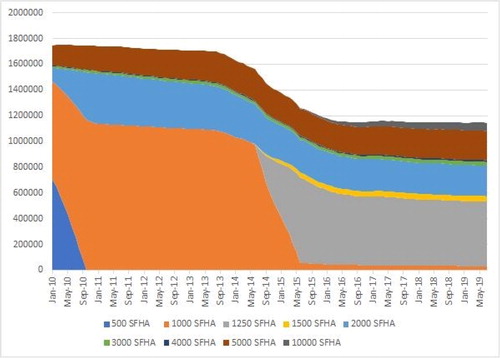
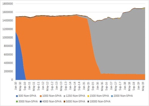
Figure 2. Total non-SFHA policies by deductible (January 2010 – July 2019).

Note. Figure 2 presents the total number of National Flood Insurance Program policies by deductible ($500, $1,000, $1,250, $1,500, $2,000, $3,000, $4,000, $5,000, or $10,000) in effect by month from January 2010 through July 2019 for owner-occupied single-family dwellings that are outside of Special Flood Hazard Areas. This stacked line graph makes obvious a) the raising of the minimum deductible from $500 to $1000, and b) the raising of the minimum from $1,000 to $1,250 for building coverage greater than $100,000. The figure is dominated by Preferred Risk Policies which constitute over 90% of the non-SFHA policies in our sample.

Figure 1 presents the total number of SFHA policies stacked by deductibles that were in effect from January 2010 through July 2019 by month. We consider a policy to be in effect for the month if its Effective Date is earlier than or equal to the first day of the month and its Termination Date is later than or equal to the last day of the month. The color version of our stacked line graph first makes obvious the raising of the minimum deductible from $500 to $1,000. An SFHA policy is considered voluntary if it is not mortgaged or if the mortgage is not government-backed. We do not have any way of determining the number of SFHA policies that are voluntary. Second, the graph demonstrates the raising of the minimum from $1,000 to $1,250, third the availability of the $1,500 deductible, and fourth the raising of the maximum deductible from $5,000 to $10,000 on April 1, 2015. Figure 1 also reveals the 27% drop in the number of policies in effect during the two year period following the implementation of Biggert-Waters Flood Insurance Reform Act of 2012.

Figure 2 presents the total number of non-SFHA owner-occupied SFD policies stacked by deductibles that were in effect from January 2010 through July 2019 by month. As Table 2 Panels C and D indicate, PRPs compose over 90% of non-SFHA policies, dominating Figure 2. The color version of the stacked line graph makes obvious: (a) the raising of the minimum deductible from $500 to $1000; and (b) the raising of the minimum from $1,000 to $1,250 for PRPs with building coverage greater than $100,000.

The percentage of SFHA policies in effect at the minimum deductible on a month-by-month basis from January 2010 through July 2019 is presented in Figure 3. The month of October 2010 has largest percentage (87%) of SFHA policies at the minimum. Figure 3 reveals a steady decline until July 2019 when the percentage of policies at the minimum reaches 62%.

Figure 3. Minimum deductible choice in SFHAs percentage of owner-occupied SFDs.

Note. Figure 3 presents the time series for the percentage of SFHA policies in effect that have the minimum deductible available for the given properties. The minimum deductible option depends on a variety of factors, including the amount of building coverage and whether the property is pre-FIRM, post-FIRM, or part of the Emergency Program. For more details regarding the menu of deductible options over this time frame and what minimum deductibles are applied, see Table 1.

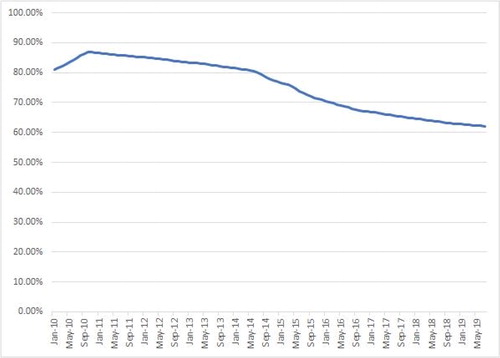
Figure 4. Maximum deductible choice in SFHAs percentage of owner-occupied SFDs.

Note. Figure 4 presents the time series for the percentage of SFHA policies in effect that have the maximum deductible available. Prior to April 2015, the maximum deductible option for SFHA properties was $5,000, and beginning in April 2015, a new maximum of $10,000 was made available. The drop in the percentage of policies at the maximum deductible in April 2015 reflects this change, and the slow take-up of this new maximum is demonstrated by the subsequent increase.

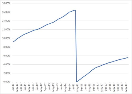
The examination of the changes to the distribution of deductibles in effect following the changes to the deductible options can also provide some information regarding the stickiness of existing policies. Figure 4 demonstrates one aspect of this stickiness where the increase to the maximum deductible in April 2015 results in a drastic drop in the percentage of policies at the maximum. Although a substantial drop may be expected, the slow conversion to the $10,000 deductible demonstrates the stickiness of the $5,000 option.

Figures 5 and 6 show the combined effect of the policyholders who chose either a $5,000 deductible or a $10,000 deductible. Prior to April 1, 2015, Figure 5 presents​ the percentage of policies that were at the maximum $5,000 deductible. Beginning April 1, 2015, Figure 5 includes the $10,000 deductible policies in addition to the $5,000 deductible policies. Together with Figure 3, Figure 5 shows the general trend for higher deductible choices. As the choice for a higher deductible gradually increases from about 9% of properties to nearly 25% of properties, the decision for the minimum deductible steadily decreases from over 80% to about 62% of policies. Figure 6 provides a stacked line graph of the absolute count of policies, rather than percentages. Figures 5 and 6 taken together reveal that, while the total number of policies decrease in general after Biggert-Waters, the percentage of policies written at higher deductibles continue to increase.

Figure 5. $5,000 and $10,000 deductibles in SFHAs: Percentage of policies in effect before and after April 1, 2015 owner-occupied SFDs.

Note. Figure 5 presents the time series for the percentage of SFHA policies that had either a $5,000 or $10,000 deductible. This plot is identical to the one in Figure 4 up until the increase to the maximum deductible in April 2015. For the subsequent period, the percentage includes policies with either the old maximum of $5,000 or the new maximum of $10,000.

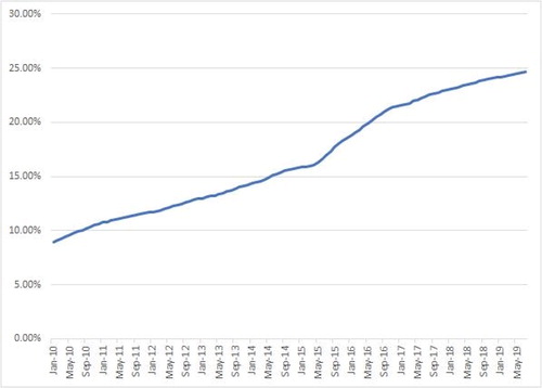
Figure 6. $5,000 and $10,000 deductibles in SFHAs: Count of policies in effect before and after April 1, 2015 owner-occupied SFDs.

Note. Figure 6 presents the total counts for SFHA policies with either $5,000 or $10,000 deductibles. This plot demonstrates the reduction in policies following the implementation of Biggert-Waters in October 2014, and then the take-up of the $10,000 deductible option after it was made available in April 2015. After the addition of the new maximum option, it can be seen that the majority of the policy growth since 2015 can be attributed to the $10,000 option.

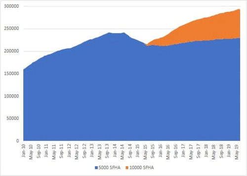
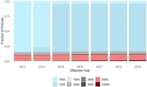
Figure 7. Distribution of deductibles by year (for our 252,280 matched policies).

Regression Analysis

For our empirical analysis of the deductible choices of policyholders, we begin by identifying policies from 2013 for single-family owner-occupied residences located within an SFHA. Since most non-SFHA properties are eligible for a PRP, which only has a single deductible option, the SFHA policies provide a meaningful amount of variation in deductibles for examination.

With this initial set of policies, we identify the subsequent policies for these properties using the following set of variables: census tract, original policy date, construction date, city, longitude (one decimal degree), latitude (one decimal degree), and number of floors. Using these variables to match subsequent policies, we are able to trace 252,280 policies throughout the 2013–2019 period. Table 3 presents summary statistics for these matched policies. The statistics reported are for the year 2015. The mean coverage in 2015 is $252,614 and the mean cost for $100,000 worth of coverage is $537. Sixty-three percent of the policies have contents coverage and 80% of the sample is in coastal states (Texas to Maine). Figure 7 depicts the distribution of deductible choices for these policies annually from 2013 to 2019.

The most substantial change to the distribution of deductibles in Figure 7 results from the increase in the minimum deductible from $1,000 to $1,250 in June 2014. However, the roughly 5% of policies with a $1,000 deductible after 2014 demonstrates the stickiness of the deductible choice, since policyholders that had the $1,000 deductible prior to the change were able to keep this level for future renewals. Perhaps if the policyholders that switched from $1,000 to $1,250 were aware that they could keep the lower option, then this proportion may have been even larger.

Similarly, the addition of the $10,000 deductible option in April 2015 is evident in Figure 7, with the red bar at the bottom slowly capturing some of the market share from the $5,000 deductible option. Figure 8 shows the cumulative share of policyholders that had a $5,000 deductible in 2013 that switched to the new maximum of $10,000 after it was made available. As seen in Figure 8, the transition to the new maximum occurred gradually, as opposed to suddenly, once the option was made available.

Figure 8. Fraction of individuals at the $5k deductible who chose to switch to the $10k deductible (252,280 matched policies).

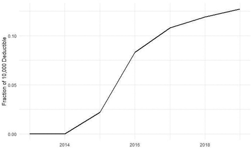
Figure 9. Premiums paid by those at the maximum deductible (252,280 matched policies).

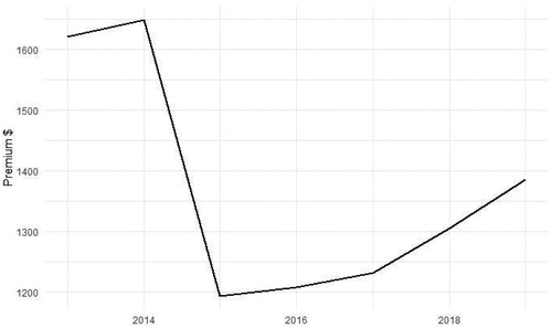
Figure 10. Selection of the maximum deductible by risk level.

Note. Figure 10 plots the estimates of β from Equation (1)(1) $$Ma{x}_{\mathit{its}}={\beta }_{}\times x+{\mu }_s+{\mu }_t+\epsilon$$(1) where the independent variable is the binned flood insurance premium for a policy with the maximum coverage and minimum deductible. The estimates for each bin indicator are plotted along with the corresponding 95% confidence interval derived from the standard errors, which are clustered at state level. The sample includes all the SFHA policies in the main analytic sample.

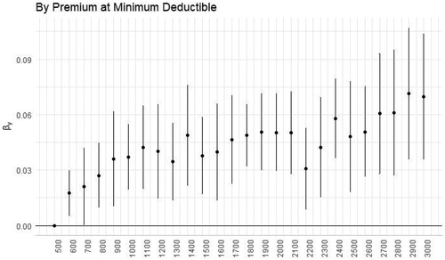
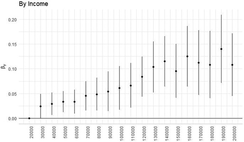
Figure 11. Selection of the maximum deductible by income level.

Note. Figure 11 plots the estimates of β from Equation (1)(1) $$Ma{x}_{\mathit{its}}={\beta }_{}\times x+{\mu }_s+{\mu }_t+\epsilon$$(1) where the independent variable is the binned median income in the corresponding census tract. The estimates for each bin indicator are plotted along with the corresponding 95% confidence interval derived from the standard errors, which are clustered at state level. The sample includes all the SFHA policies in the main analytic sample.

As can be seen in Figure​ 9, there is a substantial premium drop of about $450 for policyholders who switch to the new maximum. The figure shows that the average premium for policyholders at the maximum deductible sees a sharp drop in 2015 when the maximum deductible switches from $5,000 to $10,000. Despite this significant drop in premium, less than 20% of the policyholders choose to switch to the new maximum. Next, we examine which factors contributed to policyholders' decisions regarding whether or not to switch to the maximum.

To examine the determinants of flood insurance deductible choice, we make use of the median income and percentage of college graduates at the census tract level from the American Community Survey 5-year estimates. We expect homeowners with higher incomes are more likely to reduce annual premiums by choosing the maximum deductible (and to switch to the $10,000 deductible when available) since they can afford to pay a higher deductible in the event of a flood. We also expect that more educated people are less likely to pick the default deductible option, as they are more likely to be financially literate and may be in a better position to evaluate the costs and benefits of their deductible choices. Additionally, we proxy the census tract level cost of flood insurance by the premium of a policy with the maximum coverage and minimum deductible. Lastly, we create a variable for the claim history in a given census tract using the mean of the fraction of policies that have any claims in the previous three years. This variable serves as a proxy for the probability of future flood events. People who recently experienced a flood event are more likely to be risk averse and assign a higher probability to future flood events, leading to lower deductible amounts (Gallagher, 2014).

Who Chooses the Maximum Deductible?

We start by analyzing the policyholder’s decision to choose the maximum deductible coverage at the time of policy origination. This is accomplished with the following fixed effects regression specification using the policy-year panel data sample that we constructed: (1) $$Ma{x}_{\mathit{its}}={\beta }_{}\times x+{\mu }_s+{\mu }_t+\epsilon$$(1) where the subscripts of i, t, and s refer to the policy, year, and state of the observation respectively. The dependent variable Max_its indicates whether the deductible for policy i is $5,000 or more in year t. The independent variable x represents the characteristic of interest. μ_s and μ_t refer to state and time fixed effects respectively, and ε is an error term.¹² We cluster standard errors at state level.

The regression results in Tables​ 4 and 5 present the estimated marginal effects for the linear probability model in Equation (1)(1) $$Ma{x}_{\mathit{its}}={\beta }_{}\times x+{\mu }_s+{\mu }_t+\epsilon$$(1) for each of the following characteristics: flood insurance premiums for a policy with the maximum coverage and minimum deductible, median income in the census tract, percentage of the population with a college degree at the census tract level, and mean percentage of policies with claims in the prior three years. Of these results, only the estimates for the premium and median income produce statistically significant coefficients. This suggests that homeowners of properties in higher premium areas are more likely to select the maximum deductible option. Additionally, homeowners with higher incomes are more likely to select the maximum deductible. This is consistent with higher income borrowers being more capable of individually managing the losses from mild to moderate disasters and simply wishing to insure against major losses.

Table 5 estimates Equation (1)(1) $$Ma{x}_{\mathit{its}}={\beta }_{}\times x+{\mu }_s+{\mu }_t+\epsilon$$(1) using a logistic regression model and finds similar results for the premium and median income. The logistic regression also finds a significant negative relationship between education level and the likelihood of selecting the maximum deductible. Although the fraction of claims loads significantly in the univariate results, its significance dissipates in the multivariate regression in Column 5.

Table 5. Logistic regression models for selecting the maximum deductible option.

	Dependent Variable: Max Deductible
	(1)	(2)	(3)	(4)	(5)
log(Policy premium) (s.e.)	0.314*** (0.007)				0.519*** (0.009)
log(Median income) (s.e.)		0.412*** (0.007)			0.506*** (0.009)
Fraction with a college degree (s.e.)			−0.900*** (0.049)		−0.234*** (0.057)
Fraction of claims (s.e.)				0.097*** (0.034)	0.038 (0.035)
Fixed Effects	State, Year	State, Year	State, Year	State, Year	State, Year
Observations	1,350,973	1,328,826	1,326,537	1,096,904	1,096,904

Note. This table presents the regression estimates for the logistic regression model described in Equation (1)(1) $$Ma{x}_{\mathit{its}}={\beta }_{}\times x+{\mu }_s+{\mu }_t+\epsilon$$(1) . In each regression, the dependent variable is an indicator equal to one if a policy has the maximum available deductible, and zero otherwise. The independent variables refer to proxies for the risk level of a property, policyholder income, education, and prior claims history respectively.

*p < 0.1.

**p < 0.05.

***p < 0.01.

For more clarity on these relationships, Figures 10–13 present the linear probability model regression results where each of the characteristics are separated into various bins. Specifically, we bin the independent variable x​ into equal-sized bins as indicated by the horizontal axis of the plot and use dummy variables to represent each bin in Equation (1)(1) $$Ma{x}_{\mathit{its}}={\beta }_{}\times x+{\mu }_s+{\mu }_t+\epsilon$$(1) in place of the continuous variable x​ ​. These figures allow us to understand the exact nature of the relationship and the impact of outliers on the regression estimates in Tables 4 and 5. These figures plot the coefficient estimates of these dummy variables and the corresponding 95% confidence intervals. The standard errors are clustered at state level. The upward trend in Figure 10 suggests that the relationship in Table 4 Column 1 is robust; individuals who pay a higher premium are more likely to select the maximum deductible option. Figure 11 confirms that homeowners with higher incomes opt for the maximum deductible more often than lower-income homeowners.

Table 4. Linear probability models for selecting the maximum deductible option.

	Dependent Variable: Max Deductible
	(1)	(2)	(3)	(4)	(5)
log(Policy premium) (s.e.)	0.040*** (0.010)				0.068**** (0.010).
log(Median income) (s.e.)		0.049*** (0.014)			0.064**** (0.013)
Fraction with a college degree (s.e.)			−0.109 (0.068)		−0.027 (0.073)
Fraction of claims (s.e.)				0.008 (0.028)	−0.002* (0.024)
Fixed Effects	State, Year	State, Year	State, Year	State, Year	State, Year
Observations	1,350,973	1,328,826	1,326,537	1,096,904	1,096,904
Adjusted R^2	0.063	0.063	0.061	0.054	0.059

Note. This table presents the regression estimates for the linear probability model described in Equation (1)(1) $$Ma{x}_{\mathit{its}}={\beta }_{}\times x+{\mu }_s+{\mu }_t+\epsilon$$(1) . In each regression, the dependent variable is an indicator equal to one if a policy has the maximum available deductible, and zero otherwise. The independent variables refer to proxies for the risk level of a property, policyholder income, education, and prior claims history respectively. Standard errors are clustered at state level.

*p < 0.1.

**p < 0.05.

***p < 0.01.

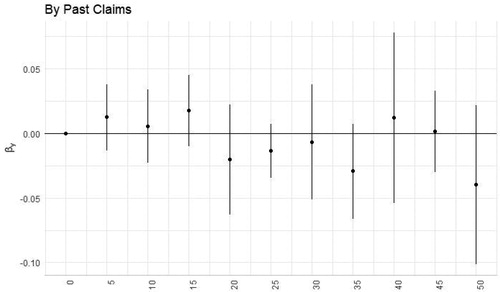
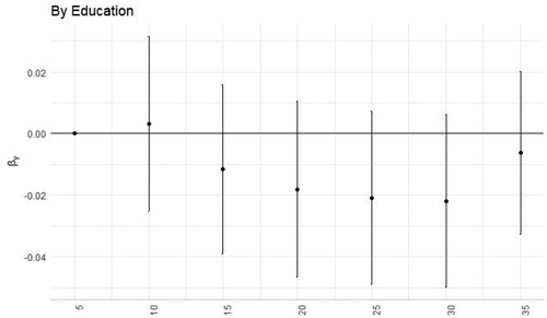
The results in Figure 12 for the proportion of college educated homeowners in a census tract do not appear to show any clear pattern, and none of the bins produce a coefficient significantly different from zero. Similarly, the results in Figure 13 for the mean percentage of policies with claims in the prior three years do not show any significant impact on the likelihood of homeowners to select the maximum deductible option.

Who Increases to a New Maximum Deductible When the Limit is Increased?

The addition of a $10,000 deductible option beginning in April 2015 provides a setting where we can further examine which homeowners prefer to select the maximum available option. Beginning with the set of policies that were active from 2013 to 2019, we identify those that had a $5,000 deductible prior to 2015, and examine the proportion of those policies that switch to the $10,000 deductible option in the years following its availability. This is accomplished with the following cross-sectional regression estimated using the cross section of policies in 2019: (2) $$d1{0000}_{is}=\mathrm{ }{\beta }_{}\times x+\mathrm{ }{\mu }_s+\mathrm{ }\epsilon$$(2) where all of the variables on the right side are identical to those in Equation (1)(1) $$Ma{x}_{\mathit{its}}={\beta }_{}\times x+{\mu }_s+{\mu }_t+\epsilon$$(1) , the independent variable d10000_its is an indicator of whether the deductible for policy i is $10,000 in year 2019, and ε is an error term.

Table 6 presents the results for the linear probability model for the same four characteristics from the previous section. Table 7 presents the logistic regression estimates. Of these results, the income variable produces an estimate that is positive and statistically significant. This is again consistent with the idea that homeowners with higher incomes are more capable of withstanding the losses from low- to moderate-severity disasters and aiming to minimize their premiums to only insure against major disasters. Although the premium is significant in univariate regressions, it is insignificant in the multivariate cases. In the logistic regressions, the fraction of claims produces a significant negative result, which suggests that homeowners that experienced recent flood damage are less likely to increase to the new maximum deductible. This is consistent with the idea from Gallagher (2014) that people with recent flood experiences are more likely to be risk averse, assign a higher probability to future flood events, and opt for lower deductible amounts.

Table 6. Linear probability models for switching from $5,000 to $10,000 deductible.

	Dependent Variable: New Max Deductible
	(1)	(2)	(3)	(4)	(5)
log(Policy premium) (s.e.)	−0.009** (0.004)				−0.0004 (0.005)
log(Median income) (s.e.)		0.033*** (0.009)			0.036*** (0.008)
Fraction with a college degree (s.e.)			0.043 (0.074)		0.093 (0.061)
Fraction of claims (s.e.)				−0.025 (0.026)	−0.030** (0.013)
Fixed Effects	State	State	State	State	State
Observations	37,834	36,772	36,679	30,105	30,105
Adjusted R^2	0.004	0.005	0.004	0.005	0.006

Note. This table presents the regression estimates for the linear probability model described in Equation (2)(2) $$d1{0000}_{is}=\mathrm{ }{\beta }_{}\times x+\mathrm{ }{\mu }_s+\mathrm{ }\epsilon$$(2) . In each regression, only policies that had a deductible of $5,000 (the old maximum) prior to April 2015 are included. The dependent variable is an indicator equal to one if a subsequent policy for the same property switches to the new maximum ($10,000), and zero otherwise. The independent variables respectively refer to proxies for the risk level of a property, policyholder income, education, and prior claims history. Standard errors are clustered at state level.

*p < 0.1.

**p < 0.05.

***p < 0.01.

Table 7. Logistic regression models for switching from $5,000 to $10,000 deductible.

	Dependent Variable: New Max Deductible
	(1)	(2)	(3)	(4)	(5)
log(Policy premium) (s.e.)	−0.082*** (0.009)				−0.006 (0.041)
log(Median income) (s.e.)		0.323*** (0.049)			0.368*** (0.054)
Fraction with a college degree (s.e.)			0.300 (0.315)		1.009*** (0.341)
Fraction of claims (s.e.)				−0.226*** (0.087)	−0.344*** (0.088)
Fixed Effects	State	State	State	State	State
Observations	37,834	36,772	36,679	30,105	30,105

Note. This table presents the logistic regression estimates for the model described in Equation (2)(2) $$d1{0000}_{is}=\mathrm{ }{\beta }_{}\times x+\mathrm{ }{\mu }_s+\mathrm{ }\epsilon$$(2) . In each regression, only policies that had a deductible of $5,000 (the old maximum) prior to April 2015 are included. The dependent variable is an indicator equal to one if a subsequent policy for the same property switches to the new maximum ($10,000), and zero otherwise. The independent variables refer to proxies for the risk level of a property, policyholder income, education, and prior claims history respectively. Standard errors are clustered at state level.

*p < 0.1.

**p < 0.05.

***p < 0.01.

Figures 14–17 present the regression results for the four characteristics when separated in various bins. As before, we use dummy variables to represent each bin and figures plot the coefficient estimates and corresponding 95% confidence intervals. Of these results, the most notable comes from Figure 15 where census tracts with median incomes of $180,000+ are substantially more likely to increase from the $5,000 deductible to the new maximum of $10,000. Again, this aligns with the idea that these high-income homeowners are more capable of bearing the risk of mild disasters and simply wish to minimize premiums or reduce the likelihood of having to go through an arduous claims process.

Figure 13. Selection of the maximum deductible by claim history.

Note. Figure 13 plots the estimates of β from Equation (1)(1) $$Ma{x}_{\mathit{its}}={\beta }_{}\times x+{\mu }_s+{\mu }_t+\epsilon$$(1) where the independent variable is the binned mean percentage policies with claims in the previous three years. The estimates for each bin indicator are plotted along with the corresponding 95% confidence interval derived from the standard errors, which are clustered at state level. The sample includes all the SFHA policies in the main analytic sample.

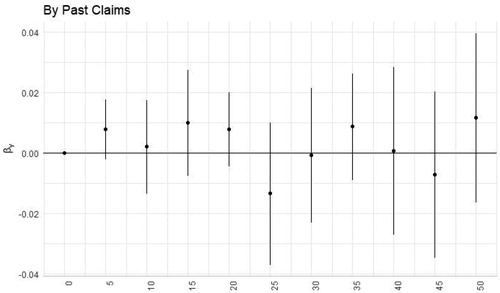
Figure 14. Likelihood of increasing deductible to new maximum by risk level.

Note. Figure 14 plots the estimates of β from Equation (2)(2) $$d1{0000}_{is}=\mathrm{ }{\beta }_{}\times x+\mathrm{ }{\mu }_s+\mathrm{ }\epsilon$$(2) where the independent variable is the binned flood insurance premium for a policy with the maximum coverage and minimum deductible. The estimates for each bin indicator are plotted along with the corresponding 95% confidence interval derived from the standard errors, which are clustered at state level. The sample includes all the SFHA policies in the main analytic sample that are active from 2013 to 2019 and are observed to have a $5,000 deductible prior to 2015.

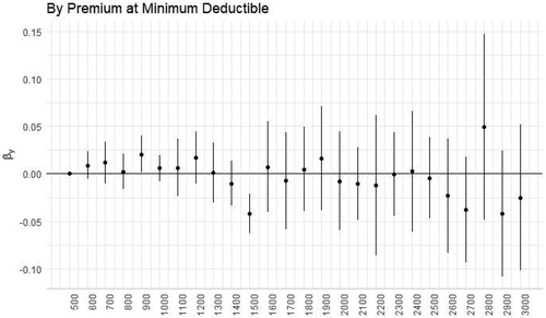
Figure 15. Likelihood of increasing deductible to new maximum by income level.

Note. Figure 15 plots the estimates of β from Equation (2)(2) $$d1{0000}_{is}=\mathrm{ }{\beta }_{}\times x+\mathrm{ }{\mu }_s+\mathrm{ }\epsilon$$(2) where the independent variable is the binned median income in the corresponding census tract. The estimates for each bin indicator are plotted along with the corresponding 95% confidence interval derived from the standard errors, which are clustered at state level. The sample includes all the SFHA policies in the main analytic sample that are active from 2013 to 2019 and are observed to have a $5,000 deductible prior to 2015.

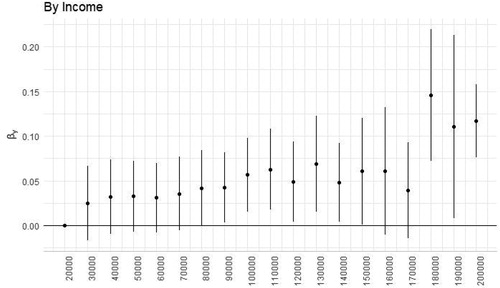
Figure 16. Likelihood of increasing deductible to new maximum by education level.

Note. Figure 16 plots the estimates of β from Equation (2)(2) $$d1{0000}_{is}=\mathrm{ }{\beta }_{}\times x+\mathrm{ }{\mu }_s+\mathrm{ }\epsilon$$(2) where the independent variable is the binned percentage of the population with a college degree at the census tract level. The estimates for each bin indicator are plotted along with the corresponding 95% confidence interval derived from the standard errors, which are clustered at state level. The sample includes all the SFHA policies in the main analytic sample that are active from 2013 to 2019 and are observed to have a $5,000 deductible prior to 2015.

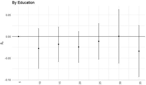
Figure 17. Likelihood of increasing deductible to new maximum by claim history.

Note. Figure 17 plots the estimates of β from Equation (2)(2) $$d1{0000}_{is}=\mathrm{ }{\beta }_{}\times x+\mathrm{ }{\mu }_s+\mathrm{ }\epsilon$$(2) where the independent variable is the binned mean percentage policies with claims in the previous three years. The estimates for each bin indicator are plotted along with the corresponding 95% confidence interval derived from the standard errors, which are clustered at state level. The sample includes all the SFHA policies in the main analytic sample that are active from 2013 to 2019 and are observed to have a $5,000 deductible prior to 2015.

Discussion: Deductible Choice and Insurance Take-up

The menu of deductible choices offered by the NFIP may have an impact on bringing in the newly insured and improving take-up rates. One such example is when the variety of deductible options was expanded effective April 1, 2015 and the maximum allowable deductible was increased from $5,000 to $10,000. This higher deductible option may attract new customers in more ways than one. Most directly, this higher deductible may attract high-income homeowners who aim to minimize their premiums or simply wish to insure against major disasters and avoid the complicated claims process for mild to moderate damage.

Another way that the expanded deductible menu may impact take-up rates for flood insurance is through publicity (the week including April 1 is the third highest spike in search interest for “flood insurance deductible,” as per Google Trends). Even if a SFHA homeowner is not interested in a $10,000 deductible or is eligible for a PRP, it is possible that mention of the additional deductible option sparked an interest in the topic. This might explain a smaller, indirect increase to flood insurance demand and lead to take-up rates for other deductible options or PRPs.

As FEMA aims to improve flood insurance take-up rates and if one of the goals of this increased deductible choice is to encourage participation in the NFIP, then an examination of this new option may shed some light on its ability to stimulate quantity demanded. When examining the take-up of the new $10,000 deductible option, it is important to distinguish between existing policyholders that decide to switch to the new option and new customers who are taking up a new policy.

The selection of flood insurance deductibles is unlikely to be a random assignment across borrowers. Although most non-SFHA homeowners are eligible for PRP policies, examination of deductible choice among SFHA homeowners reveals some interesting facts regarding who selects each of the various deductible options.

Conclusion

The viability of and costs associated with NFIP insurance are important to a well-functioning housing market. When congressional authorization for the NFIP lapsed in June 2010, the number of home transactions that were canceled or delayed in SFHAs was greater than 1,400 per day on average for the month.¹³ This disturbance to the housing market during the lapse was a result of the mandate that homeowners with federally-backed mortgages buy flood insurance for SFHA properties. The unavailability of NFIP flood insurance created a barrier for many would-be purchasers.

On October 1, 2013, as Biggert-Waters began to take effect, the housing market experienced difficulties in several areas of the country.¹⁴ Faced with the expectation of increases in premiums, many deals became infeasible. The total number of NFIP Policies in effect within SFHAs dropped over 27% during the two-year period beginning September 2013, consistent with movement toward private flood insurance.

From the threat of another lapse, to the likelihood of new congressional rules, to questions about the potential FIRM changes, the NFIP is surrounded by uncertainty. In addition, there are persistent funding issues. Due to the gap between premiums collected and claims paid, the National Flood Insurance Fund is over $20 billion in debt. Many solutions to these and other NFIP problems have been proposed.¹⁵ Rather than radical solutions, perhaps smaller fixes such as altering the available menu of deductibles might increase the health of the NFIP while preserving its valuable insurance function (e.g., Frame, 2001).

Our analysis of flood insurance deductible choice begins with 33,850,603 NFIP policies for owner-occupied single-family dwellings. We take advantage of the publicly available data with effective start dates from January 1, 2009 to June 19, 2020.¹⁶ Our results reveal that the percentage of SFHA policies in​ effect ​at the minimum deductible from January 2010 through July 2019 peaked at 87% in October 2010 and gradually declined to 62% by July 2019. Over the same time period, the percentage of SFHA policies at the maximum deductible of $5,000 grew steadily from 9% during January 2010 to 16% in March 2015. For the month that the maximum deductible was increased from $5,000 to $10,000 in April 2015, the policies at the new maximum deductible understandably plummeted to 0.01%. However, the percentage of $10,000 deductible policies continuously grew to 5.58% by July 2019. When considered together, the SFHA policies in effect at either the $5,000 or $10,000 level grew from 9% to 25% from January 2010 to July 2019, indicating a growing demand for high-deductible policies among owner-occupied single-family dwellings in SFHAs over the period. For the non-SFHA properties, approximately 10% are non-PRP, meaning that the deductible is set at either $1,000 or $1,250, depending on building coverage and time. For the non-SFHA non-PRPs, the average deductible was $1,588.28.

So who chooses the maximum deductible? Generating a matched sub-sample of 252,280 policies that we follow from 2013 to 2019, we find that those in higher flood risk locations are more likely to choose the maximum deductible. Additionally, individuals with higher income are also more likely to choose the maximum. However, homeowners who live in areas with higher disaster claims in the past three years are less likely to choose the maximum.

Who took the initiative to switch to the new $10,000 deductible? Again, using our matched sub-sample and identifying those at the $5,000 maximum deductible prior to April 1, 2015, we were able to identify that individuals with higher incomes were more likely to switch.

Since our data contains effective policy start date for policies effective January 1, 2009 and beyond, we do not know the number of policies that are “in effect” during 2009. Therefore, it is necessary for us to begin the monthly analysis starting January 2010. Those in higher-premium areas were less likely to switch;¹⁷ however, this result diminishes in a multivariate setting. Lastly, homeowners who lived in areas that experienced disasters in the last three years were less likely to switch.

A mandate within Biggert-Waters was that FEMA investigate the possibility of private market assistance. Since then, there have been interesting developments. During February 2020, FloodSmart Re Ltd. issued a $300 million catastrophe bond (Series 2020-1), joining two others from 2018 and 2019 which provide capital market reinsurance coverage for the NFIP. The private market has developed parametric insurance for disasters based upon trigger events.¹⁸ StormPeace, a private parametric insurer, promises payments within 24–72 hours based only on strength of a named storm and distance of the storm from the insured. The insured receives quick payment with no deductible and without the need for an adjuster.¹⁹

Should Risk Ratings 2.0 go farther in expanding deductible choices for greater participation? FEMA believes Risk Ratings 2.0 will help reduce the insurance gap. It may be argued that the current strategy increases premiums, but what might happen if more choices were provided? If the goal is increased take-up rates, perhaps the availability of lower premium options (higher deductibles) would be a better strategy toward those who do not currently believe they need insurance. Rather than not having flood insurance at all, a higher deductible plan would allow non-participants to better control costs. Additionally, current participants contemplating allowing their flood insurance to lapse would have an intermediate option between no insurance and insurance with a low deductible. Given nudge theory and stickiness, should FEMA continue to guide the PRP insured towards having a single low-deductible?

Figure 12. Selection of the maximum deductible by education level.

Note. Figure 12 plots the estimates of β from Equation (1)(1) $$Ma{x}_{\mathit{its}}={\beta }_{}\times x+{\mu }_s+{\mu }_t+\epsilon$$(1) where the independent variable is the binned percentage of the population with a college degree at the census tract level. The estimates for each bin indicator are plotted along with the corresponding 95% confidence interval derived from the standard errors, which are clustered at state level. The sample includes all the SFHA policies in the main analytic sample.

Notes

Notes

1 “Everyone Lives in a Flood Zone” (updated January 3, 2018). https://www.fema.gov/news-release/2007/06/21/everyone-lives-flood-zone

2 The number would surpass $36 billion if not for the forgiveness of $16 billion in National Flood Insurance Fund (NFIF) debt on October 26, 2017. Despite current NFIF debt levels, FEMA has never yet failed to honor existing flood insurance contracts.

3 Properties with more than one building/home require separate policies for each structure. As we refer to “property” throughout this paper, we are technically referring to a particular building for NFIP purposes.

4 We exclude 66,390 SFHA policies that are PRPs. SFHA PRPs are special cases where a) each property was previously in a non-SFHA, and b) the homeowner wisely opted to be “grandfathered in” and remain with a PRP rating (usually up to 2 years). Since these 66,390 policies are less than 0.2% of the policies, they have been excluded from our sample.

5 Risk Ratings 2.0, previously scheduled for implementation on October 1, 2020, is currently delayed one year until the anticipated date of October 21, 2021.

6 ​See https://www.fema.gov/nfiptransformation and ​https://www.fema.gov/media-library/assets/documents/183086

7 Actually, any uncertainty regarding current or future flood zone status is not harmless with regards to property valuation in general (see Chang et al., 2010).

8 See ​https://www.fema.gov/media-library/assets/documents/180376

9 The NFIP codes ​elevationDifference ​as 9999 when the elevation difference between the lowest floor used for rating and the base flood elevation is not reported and/or used for this policy. In addition to 9999, the code 999 is also used in the publicly available data.

10 Although federal law requires flood insurance in SFHAs when the mortgage is federally-backed, research has questioned​ whether the mandate is actually enforced, especially after the first year of purchase (e.g., Kousky, 2011; Landry & Jahan-Parvar, 2011; Michel-Kerjan et al., 2012; Michel-Kerjan & Kousky, 2010).

11 For early research testing the impact of subsidized and non-subsidized flood insurance on properties, see Shilling et al. (1989).

12 The included fixed effects capture some of the unobserved variation at the census tract level. However, there may still be additional local dynamic variables such as household wealth and employment status that could potentially improve the explanatory power of the regressions.

13 Horn, D. P. (2019, November 26). What Happens if the National Flood Insurance Program (NFIP) Lapses? (IN10835) U.S. Congressional Research Service.

14 Alvarez, L., & Robertson, C. (2013, Oct. 22). Cost of Flood Insurance Rises, Along with Worries. ​New York Times. https://www.nytimes.com/2013/10/13/us/cost-of-flood-insurance-rises-along-with-worries.html

15 Baen and Dermisi (2007) provide detailed recommendations for government actions and government-related activities.

16 A policy can be purchased well in advance of its effective start date.

17 ​On August 13, 2015, the U.S. Department of Homeland Security formally presented FEMA’s 381-page report to Congress. ​https://www.artemis.bm/deal-directory/floodsmart-re-ltd-series-2020-1/

18 ​Van Nostrand and Nevius (2011) explain that parametric insurance is a promising alternative for traditional insurance because of its immediate availability after a disaster.

19 In fact, it is not even necessary that the insured has sustained any damages.​

References

- Baen, J., & Dermisi, S. (2007). The New Orleans-Katrina case for new federal policies and programs for high-risk areas. Journal of Real Estate Literature, 15(2), 229–252.
- Beshears, J., Choi, J. J., Laibson, D., & Madrian, B. C. (2009). The importance of default options for retirement saving outcomes: Evidence from the United States. In Social security policy in a changing environment (pp. 167–195). University of Chicago Press.
- Blanchard-Boehm, R. D., Berry, K. A., & Showalter, P. S. (2001). Should flood insurance be mandatory? Insights in the wake of the 1997 New Year’s Day flood in Reno–Sparks, Nevada. Applied Geography, 21(3), 199–221.
- Botzen, W. W., & van den Bergh, J. C. (2012). Risk attitudes to low-probability climate change risks: WTP for flood insurance. Journal of Economic Behavior & Organization, 82(1), 151–166.
- Bradt, J. (2019). Comparing the effects of behaviorally informed interventions on flood insurance demand: An experimental analysis of ‘boosts’ and ‘nudges’. Behavioural Public Policy, 1–31.
- Brough, A., Isaac, M., & Chernev, A. (2008). The “sticky choice” bias in sequential decision-making. ACR North American Advances.
- Browne, M. J., & Hoyt, R. E. (2000). The demand for flood insurance: Empirical evidence. Journal of Risk and Uncertainty, 20(3), 291–306.
- Burrus, R., Dumas, C., & Graham, E. (2008). Coastal homeowner responses to hurricane risk perceptions. Journal of Housing Research, 17(1), 49–60.
- Chang, C. H., Dandapani, K., & Johnson, K. (2010). Flood zone uncertainty and the likelihood of marketing success. Journal of Housing Research, 19(2), 171–184.
- Cohen, A,, & Einav, L. (2007). Estimating risk preferences from deductible choice. American Economic Review, 97(3), 745–788.
- Collier, B., Schwartz, D., Kunreuther, H., & Michel-Kerjan, E. (2019). Characterizing households' large (and small) stakes decisions: Evidence from flood insurance. SSRN. https://papers.ssrn.com/sol3/papers.cfm?abstract_id=3506843
- DellaVigna, S., & Malmendier, U. (2006). Paying not to go to the gym. American Economic Review, 96(3), 694–719.
- Dombrowski, T., Ratnadiwakara, D., & Slawson Jr, V. C. (2019). The FIMA NFIP’s redacted policies and redacted claims data sets. SSRN. https://papers.ssrn.com/sol3/papers.cfm?abstract_id=3464626
- Frame, D. E. (2001). Insurance and community welfare. Journal of Urban Economics, 49(2), 267–284.
- Gallagher, J. (2014). Learning about an infrequent event: Evidence from flood insurance take-up in the United States. American Economic Journal: Applied Economics, 206–233.
- Harrison, D., T. Smersh, G., & Schwartz, A. (2001). Environmental determinants of housing prices: The impact of flood zone status. Journal of Real Estate Research, 21(1–2), 3–20.
- Johnson, E. J., & Goldstein, D. (2003). Do defaults save lives? Science (302) 5649, 1338–1339.
- Kousky, C. (2011). Understanding the demand for flood insurance. Natural Hazards Review, 12(2), 96–110.
- Kousky, C., Kunreuther, H., Lingle, B., & Shabman, L. (2018). The emerging private residential flood insurance market in the United States. Wharton Risk Management and Decision Processes Center.
- Kousky, C., & Kunreuther, H. (2014). Addressing affordability in the national flood insurance program. Journal of Extreme Events, 1(01), 1450001.
- Landry, C. E., & Jahan‐Parvar, M. R. (2011). Flood insurance coverage in the coastal zone. Journal of Risk and Insurance, 78(2), 361–388.
- Michel‐Kerjan, E., Lemoyne de Forges, S., & Kunreuther, H. (2012). Policy tenure under the US national flood insurance program (NFIP). Risk Analysis: An International Journal, 32(4), 644–658.
- Michel‐Kerjan, E. O., & Kousky, C. (2010). Come rain or shine: Evidence on flood insurance purchases in Florida. Journal of Risk and Insurance, 77(2), 369–397.
- Morgan, A. (2007). The impact of Hurricane Ivan on expected flood losses, perceived flood risk, and property values. Journal of Housing Research, 16(1), 47–60.
- Van Nostrand, J. M., & Nevius, J. G. (2011). Parametric insurance: Using objective measures to address the impacts of natural disasters and climate change. Environmental Claims Journal, 23(3–4), 227–237.
- Petrolia, D. R., Landry, C. E., & Coble, K. H. (2013). Risk preferences, risk perceptions, and flood insurance. Land Economics, 89(2), 227–245.
- Ratnadiwakara, D., & Venugopal, B. (2019). Climate risk perceptions and demand for flood insurance. https://papers.ssrn.com/sol3/papers.cfm?abstract_id=3531380
- Rees, R., & Wambach, A. (2008). The microeconomics of insurance. Now Publishers Inc.
- Shilling, J. D., Sirmans, C. F., & Benjamin, J. D. (1989). Flood insurance, wealth redistribution, and urban property values. Journal of Urban Economics, 26(1), 43–53.
- Sunstein, C. R., & Thaler, R. H. (2003). Libertarian paternalism is not an oxymoron. The University of Chicago Law Review, 1159–1202.
- Willis, L. E. (2013). When nudges fail: Slippery defaults. The University of Chicago Law Review, 1155–1229.
- Zhang, L., & Leonard, T. (2019). Flood hazards impact on neighborhood house prices. The Journal of Real Estate Finance and Economics, 58(4), 656–674.