Do strict decision criteria hamper productivity in the pharmaceutical industry?

ABSTRACT

The discouragingly high rates of attrition in drug development, and in particular in Phase 2, warrant a closer look at the decision criteria applied for investment in the next phase (Phase 3). We have in this article evaluated Stop/Go criteria after Phase 2, based on a model encompassing both Phase 2 and 3, as well as the eventual outcome on the market. The results indicate that the value of a drug project is often maximized if rather liberal decision criteria are applied. The routine adherence to standard criteria, e.g. requiring significance at 5% level, may lead to an unduly high rate of false negative decisions. This might ultimately hamper the productivity of drug development and leading to potentially useful drugs not being taken forward to benefit the intended patients.

KEYWORDS:

• Drug development
• net present value
• productivity index
• return on investment
• false negative decisions

1. Introduction

It is a well-known fact that a majority of drug candidates will fail, not reaching the market and consequently not bring benefit to the intended patients. The highest attrition rate is found in Phase 2 and the most common reason for project failures is the lack of desired efficacy (DiMasi et al. 2016; Hay et al. 2014; Wong et al. 2019). While the highest attrition rates are found in Phase 2, the consequences in terms of both costs and number of patients involved can be even larger in Phase 3. De Martini (2020) makes the remarkable estimate that over 800 000 patients might be recruited every year to a Phase 3 trial that fails.

A great deal of attention has been given to the issue of potential false positive outcomes from Phase 2, primarily focusing on the efficacy-based failures. Pereira et al. (2012) gives an overview over projects where exceptionally good results have not been replicated in later trials, and the problem has also been studied by several other authors, e.g. Ioannidis (2005), Chuang-Stein and Kirby (2014). The U.S. Food and Drug Administration, FDA (2017) has presented a study of examples where the Phase 3 results did not correspond to what was previously seen in Phase 2. Part of the explanation for late phase disappointments is the existence of ‘regression to the mean’ effects, which several authors have paid attention to from slightly different perspectives (De Martini 2011; Kirby et al. 2012).

De Martini (2020) proposes some alternatives for remedy of the risk of Phase 3 failures. His main suggestion is on enlarging the Phase 2 trials to enable Go/NoGo decisions for starting Phase 3 to be based on more accurate data. Huang et al. (2019) arrives at a similar conclusion, stating that an increase in the sample size in Phase II will result in greater increase in success probability of Phase III than increasing the Phase III sample size by an equal amount.

Investigations as mentioned above have often focused on the disappointments and failures in Phase 3. In other words, there has been a focus on the problem of false positive decisions in Phase 2. A conclusion that is often drawn, at least implicitly, is that very high requirements should be placed on the results from Phase 2 and that strict decision criteria should be implemented for a Phase 3 investment to be made.

While much interest has been paid to the issue of false positives, the occurrence of false negatives has not been given the same attention. Just as it is easy to understand that regression to the mean can occur on the positive side, it should be obvious that it can also occur on the negative side. Phase 2 trials are typically small, leading to a large random component and a large uncertainty in the observed results. A consequence is that good drug candidates may have bad luck in Phase 2 and would have shown good results in Phase 3. The termination of such projects would correspond to false negative decisions. The occurrence and impact of such decisions are more difficult to study, simply because we do not know what the next phase outcome would have been.

This background together with the very high attrition rate in Phase 2 warrants a question to be raised: does the pharmaceutical industry in fact place too high hurdles for proceeding to later phase trials? Does the industry unnecessarily abandon many drug candidates that would have had the potential to ultimately benefit patients, should they not have been terminated early?

Miller and Burman (2018) developed a decision theoretical model for studying investment decisions and licensing approvals. Their model was built to both account for, and maximize, the revenue of both drug development sponsors, as well as the public welfare. Among the conclusions, they argued for the importance that the “consequences of type I and type II errors are factored in when determining the relation between type I and type II error rates”. Underlying this conclusion are some results indicating that the type I error rate should in many situations be much higher than the values normally selected for design and decision-making (i.e. much higher than 5%). Chen and Beckman (2009) derive a model to find optimal decision criteria for maximizing a benefit cost ratio. Their study has a particular focus on oncology trials, and the results indicate that the empirical bar to proceed from PoC trials to Phase 3 development should be substantially lower than the effect size, ∆, anticipated in the design phase. The optimal decision criteria for ∆ are shown to correspond to a type I error rate (α) that is generally higher than what is usually applied in clinical trials. Lindborg et al. (2014) build a model to evaluate the expected cost per launch of a new drug. The choice of risks for false positive (cf type I error rate, α) and false negative decision (cf type II error rate, β) in Phase 2 are then evaluated, to minimize expected cost. The authors conclude that the false positive risk should be selected substantially higher than the usual 5%, and the false negative decision risk rather lower than commonly applied. Contributions on related topics have also been made by Mudge et al. (2012), on the optimal choice of type I error from a frequentist perspective, and more recently by Walley and Grieve (2021), dealing with the trade-off between type I and II error rates in the context of a Bayesian analysis.

The findings mentioned above indicate that the existence of false negative decisions might be a larger problem than has previously been reflected in the literature, and that the current practice of strict decision criteria might be counter-productive for the sponsors and for the public welfare. It is the purpose of this paper to further investigate this issue. Our approach is not to strive for an optimal analytical solution in a model with relatively few parameters, but rather to set the issue in a context of a model that should be flexible enough to realistically represent the drug development process. As a consequence, we will use simulations to produce the numerical results.

The remainder of the article is structured as follows. The next chapter outlines the general model to be used for the evaluation, followed by a description of the simulation study conducted to generate the results. The outcome of the simulation study is then presented in a Results section and a discussion section concludes the article.

2. A model of the drug development process

2.1. General modelling concept

The main objective of this study is to evaluate the performance of a drug development process for different decision criteria. To enable a realistic evaluation, it is important to capture the key aspects of a drug project in the model on which the evaluation is based. We will to a large extent follow the modelling framework laid out by Wiklund (2019), but also borrow some aspects of the model from Miller and Burman (2018). The framework includes the following main parts:

• Cost and duration

• Treatment effect distributions

• Sample size of key clinical trials

• Criteria for stop/go decisions

• Market and sales revenue

• Outcome measures

We will in the following sections present these model components in some more detail. It may be noted already at the outset that the model as presented here does reflect standard study designs and the traditional separation of Phase 2 and Phase 3. There are obviously many cases in which the situation is different. In rare diseases and some oncology indications, early data from single arm trials are sometimes sufficient to proceed to Phase 3. Adaptive and flexible designs, often including interim analyses, are becoming more common. While it is beyond the scope of this article to tailor the model to these special cases, the proposed modeling framework should be applicable to specific situations with some appropriate adjustment to model components and numerical parameter values.

2.2. Cost and duration

The cost incurred and the time it takes to complete each phase are key components when modelling the drug development process. For each phase, j∈{2, 3}, we define the cost, C_j, and duration, T_j. The cost is modelled to be proportional to the number of patients in the key clinical trial(s) of the phase, plus a fix cost representing all other activities in this phase, i.e.

$C_j=C_j^0+N_j{C}_j^N$

where $N_j$ is the number of patients in key clinical trials, $C_j^N$ is the cost per patient and $C_j^0$ is the additional fix cost of the phase. For the registration phase, we assume a fixed cost, C_reg.

The duration of a phase is modelled to be dependent on the time it takes to recruit patients to the key trial(s) of the phase. If the recruitment rate is $Q_j$ patients per year, the duration of the phase is given by

$T_j=T_j^0+N_j/Q_j$

making the duration of a phase proportional to the sample size plus an additive component, $T_j^0$. The recruitment and sample size dependent part of the duration would typically be related to the time between ‘first patient in’ to ‘last patient in’. The additive component would capture the time for any other parts of the study, including (but not limited to) the treatment period and/or follow-up period (e.g. the time between ‘last patient in’ to ‘last patient out’). The additive component would also capture any additional activities on the critical path of the development program. It could be argued that the additive component might on average be longer when a time-to-event endpoint is used for the key clinical trial, but that would simply be accounted for by assigning a higher value to $T_j^0$ when using the model to produce numerical results. For the registration phase, we assume a fixed duration, T_reg. The parameter values assigned to the cost and duration parameters in the subsequent simulation study are summarized in Appendix, Table 1.

2.3. Treatment effect

The most common reason for the failure of drug projects is a lack of sufficient efficacy. Our model to capture this is based on assuming that the drug has a true treatment effect, $E_j$. In the clinical trials we may then estimate the efficacy, ${\hat{E}}_j$. This observed efficacy is representing the underlying true treatment efficacy, plus a random error corresponding to the standard error of the efficacy estimate, ${\hat{E}}_j=E_j+{\epsilon }_j$.

The true treatment effect is unknown, and we will model the corresponding uncertainty by assigning a stochastic (prior) distribution to $E_j$. Wiklund and Burman (2021) evaluated different choices for the distribution and based on their results we will use the lognormal distribution, $E_j\sim logN\left({\mu }_j,{\gamma }_j\right)$ in our evaluations. Additional evaluations will be made using a two-point distribution:

$E_j=\left\{\begin{array}{c}{E}_{0}withprobability{p}_j\\ 0withprobability1-p_j\end{array}\right.$

where $p_j$ denotes the probability that the project has a positive true treatment effect. The two-point distribution is consistent with the approach taken by e.g. Chen and Beckman (2009) and Mudge et al. (2012).

We will assume that the observed efficacy is representing the comparison between two treatment groups (investigational treatment versus control), and for simplicity let the analyses be approximated by the comparison of two group means. The observational error, ${\epsilon }_j$, is then approximated by a normal distribution with mean zero and the standard error being ${\sigma }_j\sqrt{2/n_j}$, where $n_j$ is the number of patients in each of the two treatment arms. While this approach is derived from the simple situation of the comparison of two group means, as noted by Miller and Burman (2018) this formulation is quite general and, due to the central limit theorem, applicable to different types of responses. Hence it may be a reasonable approximation to many of the analyses conducted in clinical development, e.g. for continuous or time-to-event data.

The parameter values assigned to the treatment effect parameters in the subsequent simulation study are summarized in Appendix, Table 3.

2.4. Sample size

The number of patients to be enrolled in the key clinical trials are calculated using standard sample size calculation formulae. As in the previous section, we will use the approximation of the comparison of two treatment means. With the two-sided significance level, $\alpha { }_j^{\prime }$, and the intended power, $1-{\beta }_j$, the sample size is calculated as

$n_j=2{\left(\frac{{\sigma }_j}{E_0}\right)}^2{\left(z_{\alpha { }_j^{\prime }/2}+z_{\beta }\right)}^2$

assuming equal allocation between treatment arms and letting $E_0$ denote the anticipated treatment effect. The parameter values that were assigned to parameters for sample size calculations in the subsequent simulation study are summarized in Appendix, Table 2.

While we have presented the modeling framework with the approximation of the standard sample size formula above, the general approach should be applicable also to other situations, given appropriate adjustment. Note that the sample size formula above can be written as

$n_j=K{\left(\frac{1}{\mathrm{\Delta }}\right)}^2{\gamma }_{{\alpha }^{\prime },\beta }^2$

where ${\gamma }_{{\alpha }^{\prime },\beta }=z_{\alpha { }_j^{\prime }/2}+z_{\beta }$ is the factor given by type I and type II errors, and $\mathrm{\Delta }=E_0/\sigma$ is the anticipated effect size. Standard formulae for sample size calculations, e.g. for time-to-event data, have the same form, with $\mathrm{\Delta }$ being the effect size often given as a log-hazard-ratio. Adapting the presented modeling framework to e.g. survival endpoints, could hence be reduced to selecting a value for K appropriate to the selected effect size parameter.

2.5. Decision criteria

A project is taken forward to Phase 3 only if it shows sufficient efficacy in a key clinical trial in Phase 2. The criterion is often based on showing a statistically significance difference between the treatment groups. A positive investment decision is then made if the p-value from a previous trial is lower than a given threshold, ${\hat{p}}_j<{\alpha }_j^{crit}$, alternatively the criterion could be defined as a test statistic, z, exceeding a given threshold, ${\hat{z}}_j>z_j^{crit}$. It could be noted at this point that our model makes the distinction between the value of α used in the sample size calculation (${\alpha }_j^{\mathrm{\prime }}$), and the threshold applied for the decision criterion (${\alpha }_j^{crit}$), and that we allow for the fact that these two parameters could be different.

The critical value for the test statistic is $z_j^{crit}=\mathrm{\Phi }\left(1-{\alpha }_j^{crit}/2\right)$, where ${\alpha }_j^{crit}$ is the significance level applied for the decision. While the significance level required for a successful progression from Phase 3 to market authorization is typically given by the regulatory authorities, there is more flexibility for a sponsor to decide on the requirements for progressing from Phase 2 to Phase 3, i.e. to decide on the value of ${\alpha }_2^{crit}$. Properties of different choices of ${\alpha }_2^{crit}$ are central to the investigations presented in this paper.

It is sometimes argued that decision criteria should not be based on statistical significance, but on clinical relevance. We may note, however, that under the applied modelling framework there is a direct relationship between criteria for significance and criteria for effect size. With the observed value of the test statistic being

${\hat{z}}_j=\frac{{\hat{E}}_j}{SE\left({\hat{E}}_j\right)}=\frac{{\hat{E}}_j}{{\sigma }_j\sqrt{2/n_j}}$

the criterion ${\hat{p}}_j<{\alpha }_j^{crit}$ is, for a given sample size, equivalent to ${\hat{E}}_j>{\sigma }_j\sqrt{2/n_j}{\mathrm{\Phi }}^{-1}\left(1-{\alpha }_j^{crit}/2\right)$, or on the scale of the normalized effect size

${\hat{\mathrm{\Delta }}}_j>\sqrt{2/n_j}{\mathrm{\Phi }}^{-1}\left(1-{\alpha }_j^{crit}/2\right)$

.

where ${\hat{\mathrm{\Delta }}}_j={\hat{E}}_j/{\sigma }_j$. Relevant parts of the Results section will present outcomes for both the case where decisions after Phase 2 are based on significance (i.e. ${\hat{p}}_2<{\alpha }_2^{crit}$) and the case where decisions are based on the observed effect size (i.e. ${\hat{\mathrm{\Delta }}}_2>{\mathrm{\Delta }}_2^{crit}$).

We have here chosen to present the modeling framework based on a simple decision criterion that declares a NoGo decision if the observed value (test statistic or effect size estimate) falls below (above) a given threshold. While this is an often-used approximation, we appreciate that many other suggestions have been made for more elaborate decision criteria, sometimes tailored to specific disease areas. Frewer et al. (2016) propose a framework combining confidence intervals and point estimates and Gould et al. (2015) take a structured approach in integrating multiple attributes for the decision-making. Lennie et al. (2021) specifically address Go/NoGo decisions for rare diseases, and Chen and Beckman (2009) discuss optimal decision criteria in the oncology setting.

Our presentation of decision criteria has so far been focused solely on efficacy. While this is the most common reason for failure, there are obviously also other causes for the termination of drug projects. We will include these in the model by assigning a probability, π_j, that the drug project is terminated in Phase j, for other reasons than efficacy. Let $P_j\sim bernoulli\left({\pi }_j\right)$ be an indicator for projects terminated for non-efficacy reasons, the combined criterion for progressing a project to the next phase is then given by the variable S_j as

$S_j=\left\{\begin{array}{c}1if{\hat{z}}_j>z_j^{crit}and{P}_j=0\\ 0otherwise\end{array}\right.$

where $P_j\sim bernoulli\left({\pi }_j\right)$. An obvious modification applies for the case when the decision is based on the observed effect size, ${\hat{\mathrm{\Delta }}}_2$. The parameter values assigned to the decision criteria parameters in the subsequent simulation study are summarized in Appendix, Table 4.

2.6. Sales revenue and discounting

To get a holistic view of the drug development process, we include a model for the sales revenue generated by the drug when (if) eventually launched to the market, which happens at time T_L. We assume a model in which the revenue, R, then increases during a ramp-up period of length T_U, after which it stabilizes at a plateau where annual revenue is A. The revenue is assumed to drop to zero when key patent expires, T_P.

$R=\left\{\begin{array}{c}A\cdot \frac{t-T_L}{T_U}\\ A\\ 0\end{array}\right.\begin{array}{c}{T}_L<t\le T_L+T_U\\ T_L+T_U<t\le T\\ T_P<t\end{array}$

We further argue that for a sales model to be realistic, it should take into account the fact that a drug shown to have a very good treatment effect is likely to generate more revenue than a drug with a mediocre effect. We will in this paper use a very simple model to describe the dependency between treatment effect and revenue, where the annual peak revenue, A, is assumed to be proportional to the observed treatment effect in Phase 3. There is also a sales forecast that predicts the revenue to be A₀ if the observed treatment effect would equal the effect specified in the target product profile, E₀. The potential annual peak revenue is then given by

$A=A_0\frac{E_3}{E_0}$

The parameter values assigned to the sales model in the subsequent simulation study are summarized in Appendix, Table 5. We appreciate that the sales model as outlined above (with a ramp-up, followed by a constant plateau and a sudden drop after patent expiry), represents a relatively crude approximation. While this approximation should be a useful model in many situations, it may be noted that examples are common where the actual sales of a drug has continued to increase over many years, and where sales has been substantial also after the expiry of initial patents. Should it be considered relevant to use a more elaborate model to represent such situations, our general modelling framework could still be used after slight modifications to the parameters of the model. The constant value of $A_0$ could be replaced by a function of time, and a non-zero residual sales could be assigned (possibly also as a function of time).

To account for the reduced time-value of future cash flows, revenues are discounted using the discount rate, λ. With revenue according to the ramp-up model given above, the discounted revenue is given by the following integrals.

$R_D=\underset{T_L}{\overset{T_L+T_U}{\int }}A\frac{t-T_L}{T_U}{e}^{-\lambda t}dt+\underset{T_L+T_U}{\overset{T_P}{\int }}A{e}^{-\lambda t}dt$

where $\lambda =ln\left(1+r\right)$. After some calculus, this leads to the discounted revenue being

$R_D=\frac{A}{{\lambda }^2{T}_U}\left\{e^{-\lambda T_L}-e^{-\lambda \left(T_L+T_U\right)}\right\}-\frac{A}{\lambda }{e}^{-\lambda T_P}$

The costs for each phase, j, are also discounted to their present values as

$C_{D,j}=\frac{C_j}{\lambda T_j}\left(e^{-\lambda {\tau }_{1,j}}-e^{-\lambda {\tau }_{2,j}}\right)$

The discounted costs are based on the assumption of a constant annual cost flow of $C_j/T_j$, and obtained by evaluating the integral

$C_{D,j}=\frac{C_j}{T_j}\underset{{\tau }_{1,j}}{\overset{{\tau }_{2,j}}{\int }}{e}^{-\lambda t}dt$

where ${\tau }_{1,j}$ and ${\tau }_{2,j}$ are the start and end, respectively, of Phase j.

The discounted revenue, R_D, as defined above gives a value that is conditional on that the drug is launched to the market. To get a measure that is adjusted for the substantial risk of project failure, we multiply the conditional revenue, R_D, by the variables, $S_j$, representing success over the phases of development.

$R_R=R_D{S}_2{S}_3{S}_{reg}$

Similarly, the risk-adjusted cost is obtained by multiplying the cost of each phase with the variables that indicate that preceding phases have been successful.

$C_R=C_{D,2}-C_{D,3}{S}_2-C_{D,reg}{S}_2{S}_3$

2.7. Outcome measures

For the evaluation of decision criteria strategies, we will primarily focus on two outcome measures:

• Expected net present value, ENPV

• Expected productivity index, EPI

The expected net present value is defined as the expected revenue minus the expected cost

$ENPV=R_R-C_R$

Since the revenue is zero for projects that are not reaching the market, the ENPV is negative in these cases. The negative size of the ENPV will depend on what phases are completed prior to termination.

The expected productivity index is defined as the expected net present value divided by the expected costs

$EPI=\frac{R_R-C_R}{C_R}$

While the ENPV measures the net value of the project, the EPI relates the value of the projects to the costs required and is consequently a measure that relates to the return on investment for the project.

3. Simulation study and model parameters

3.1. Simulation study

A simulation study was conducted, to evaluate the choice of decision criterion after Phase II, ${\alpha }_2^{crit}$, in a wide range of scenarios. For each iteration, i, of the simulation, a random value was drawn from the distribution of true treatment effects, E_ij. All parameters and properties of the model were then calculated as described in the previous section. The revenue, R_R,i, and cost, C_R,i, obtained for each iteration were then averaged to get the expected revenue as $R_R=m^{-1}\sum _i{R}_{R,i}$ and the expected cost as $C_R=m^{-1}\sum _i{C}_{R,i}$, where m is the number of iterations of the simulation. The outcome measures, ENPV and EPI, were finally obtained for each scenario.

A base case was defined as a starting point for the simulations. The parameter values used to define the base case are summarized in Appendix. The appendix includes comments and, in some cases, information on the rationale or source for the chosen value for the input parameters. In the simulation study we also evaluated a number of different scenarios, in addition to the base case. The scenarios were defined by assigning ranges of values for parameters of the model, as described in the following paragraphs.

3.2. Sample size (type II error) in Phase 2

As noted in the Introduction, some authors (e.g. De Martini 2020; Huang et al. 2019) have suggested to increase the sample size of Phase 2 to enable more accurate investment decisions for Phase 3. On the other hand, initial studies in the current research indicated that a smaller Phase 2 trial could lead to higher value of the project. To evaluate these suggestions in the context of our model, we varied the Phase 2 sample size over a range from approximately 90 to 220 patients. With other parameters fixed, the different sample sizes correspond to different values of the power of the trial. Varying the sample size in the given range was obtained by varying the type II error, ${\beta }_2$, between 10% and 40%, when calculating the sample size.

3.3. Sales revenue

If the market for the developed drug is very large, either due to a large number of patients or due to a high price attained for the drug, this might impact the optimal choice of decision strategy. When the anticipated revenue is large, it would seem reasonable to avoid false negative decisions as that might have severe consequences in terms of lost revenue opportunities. On the contrary, a small anticipated market would make it more prudent to avoid false positive decisions after Phase 2 as this might lead to costly failures in Phase 3, with little financial gain to balance the risk. Simulations are run for a range of the annual peak revenue, $A_0$, between 200 MUSD and 1 000 MUSD, with 1 000 MUSD representing the base case. As a comparison, the development cost of Phase 3 is in the base case approximately 260 MUSD.

3.4. Difference in effect size and/or variability in phase 2

The clinical trials in Phase 3 are typically conducted based on the most clinically relevant endpoint and with inclusion/exclusion criteria representing the intended patient population. In Phase 2, the sponsor may have the opportunity to select a study design (e.g. by choosing endpoints and inclusion/exclusion criteria) so as to increase the likelihood of the study being able to provide evidence of efficacy. This could be achieved by reducing the variability on the clinically relevant endpoint, or by choosing an alternative (surrogate) endpoint with a beneficial relation between anticipated treatment effect and variability. This implies that Phase 2 studies are often designed based on the assumption of a higher anticipated effect size, ${\mathrm{\Delta }}_2=E_0/{\sigma }_2$. Since sample size formulae are inversely related to the effect size, the higher anticipated effect size corresponds to the fact that sample sizes are typically lower in Phase 2 than in Phase 3. The relative difference in effect size may impact the optimal choice of decision criteria. In the simulation study base case it was assumed that anticipated effect size was ${\mathrm{\Delta }}_2=0.4$ in Phase 2 and ${\mathrm{\Delta }}_3=0.25$ in Phase 3. For the simulations we evaluated a range of ${\mathrm{\Delta }}_2$ between 0.3 and 0.6, and for each value of ${\mathrm{\Delta }}_2$, a sample size for Phase 2 was calculated. The range of ${\mathrm{\Delta }}_2$ corresponds to sample sizes approximately ranging from 70 to 280 patients in Phase 2.

4. Results

The results from the simulation study described in the previous section will be presented in graphs for the various scenarios. For each scenario, both the expected net present value, ENPV, and the expected productivity index, EPI, will be shown. The outcome measures are displayed versus a range of values for the decision criteria applied after Phase 2 to make the Phase 3 investment decision. Results are presented for both a significance based criterion, ${\alpha }_2^{crit}$, and for a criterion based on the observed effect size, ${\mathrm{\Delta }}_2^{crit}$. Results are also presented for two alternative assumptions regarding the true treatment effect distribution. The treatment effect distributions are a log-normal distribution and a two-point distribution as presented in the Treatment effect section above. The results are based on 50 000 simulations for each scenario.

4.1. Base case scenario

Results in Figure 1 show that the EPI attains a maximum for values of ${\alpha }_2^{crit}$ in the range 0.1–0.15, whereas there is a reduction in EPI for higher values of the decision criterion. The ENPV is increasing for higher values of ${\alpha }_2^{crit}$, over the evaluated range, and correspondingly increasing for lower values of ${\mathrm{\Delta }}_2^{crit}$ . (It may be noted that an effect size of ${\mathrm{\Delta }}_2=0.4$ is anticipated in the base case sample size calculation). Hence the ENPV is maximized by applying very liberal decision criteria for the Phase 3 investment decision, an outcome that is consistent across the two treatment effect distributions. The results for EPI do however differ between the effect distributions. With a log-normal distribution, the EPI is maximized for a rather strict decision criterion ${\alpha }_2^{crit}<0.05$, whereas under the two-point distribution assumption, a rather liberal criterion is optimal, ${\alpha }_2^{crit}\approx 0.2$.

Figure 1. Project outcome measures as a function of the decision criterion after Phase 2, evaluated for the model base case.

Outcome measures: Expected Net Present Value (ENPV), Expected Productivity Index (EPI).Top: Lognormal effect distribution. Bottom: Two-point effect distribution.Left: Significance decision criterion, ${\alpha }_2^{crit}$. Right: Effect size decision criterion, ${\mathrm{\Delta }}_2^{crit}$

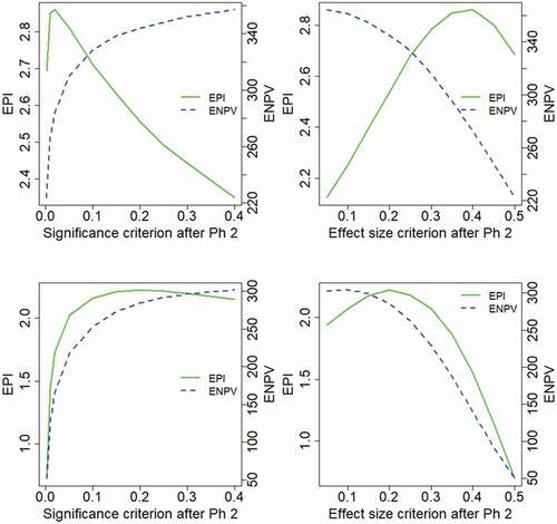
It could be noted that the optimality of ENPV for very liberal decision criteria would imply that more projects are taken forward to Phase 3, and such a strategy would require virtually unlimited resources for large Phase 3 portfolios. The results of Figure 1 also show clear differences between the properties of the two outcome measures, ENPV and EPI, and similar differences between the outcome measures are seen for many of the evaluated scenarios. The interpretation and relation between the outcome measures will be further addressed in the Discussion section. While the ENPV is a very commonly used measure of project value, we will in this article pay much attention to the results of the EPI.

Figure 2 shows the impact of choosing different levels of the type II error rate, ${\beta }_2$, applied in the Phase 2 study design. The base case scenario corresponds to ${\beta }_2=0.2$, and it may be noted that the different levels of ${\beta }_2$ correspond to the following Phase 2 sample sizes: $N_2=\left\{216,156,118,92\right\}$. An effect size of ${\mathrm{\Delta }}_2=0.4$ was anticipated for the sample size calculation. Results in Figure 2 are based on a log-normal distribution for the treatment effect-

Figure 2. Expected project value as a function of the decision criterion after Phase 2, evaluated for different levels of the type II error rate, ${\beta }_2$, applied in the Phase 2 study design.

A log-normal distribution is assumed for the treatment effect. The different levels of ${\beta }_2$ correspond to the Phase 2 sample sizes: $N_2=\left\{216,156,118,92\right\}$ Top: Expected Productivity Index (EPI). Bottom: Expected Net Present Value (ENPV).Left: Significance decision criterion, ${\alpha }_2^{crit}$. Right: Effect size decision criterion, ${\mathrm{\Delta }}_2^{crit}$

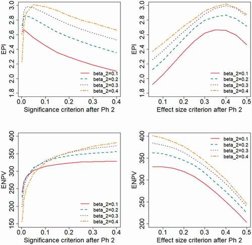
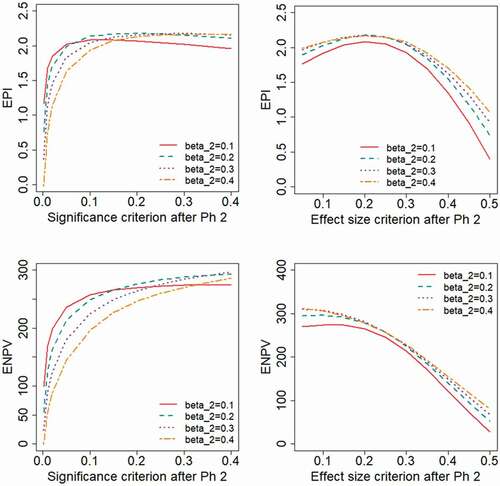
The results indicate that the highest values on the outcome measures are generally obtained for a high value of ${\beta }_2$, i.e. for a small Phase 2 sample size. The ENPV will increase by using liberal decision criteria, i.e. a high value for ${\alpha }_2^{crit}$ or a low value of ${\mathrm{\Delta }}_2^{crit}$. The EPI will instead be optimized by applying relatively strict criteria. Figure 3 shows the results for the range of type II error rate, ${\beta }_2$, when the treatment effect follows a two-point distribution. With this distribution, the EPI is maximized for more liberal decision criteria than was seen for the log-normal distribution in Figure 2. For a study designed with the power assumed in the base case (${\beta }_2=0.2$) the EPI is maximized for a significance criterion of ${\alpha }_2^{crit}\approx 0.2$, . For studies with less power (higher ${\beta }_2$) even higher values of ${\alpha }_2^{crit}$ are optimal. Also under this distributional assumption, the ENPV is maximized for liberal decision criteria.

Figure 3. Expected project value as a function of the decision criterion after Phase 2, evaluated for different levels of the type II error rate, ${\beta }_2$, applied in the Phase 2 study design. A two-point distribution is assumed for the treatment effect.

The different levels of ${\beta }_2$ correspond to the Phase 2 sample sizes: $N_2=\left\{216,156,118,92\right\}$ Top: Expected Productivity Index (EPI). Bottom: Expected Net Present Value (ENPV).Left: Significance decision criterion, ${\alpha }_2^{crit}$. Right: Effect size decision criterion, ${\mathrm{\Delta }}_2^{crit}$

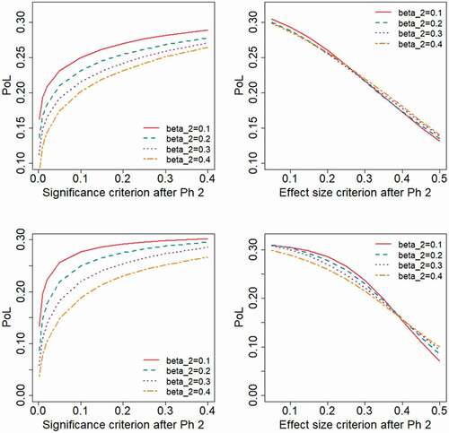
Figure 4 illustrates the probability of the project being successful through all phases of development, here referred to as the Probability of Launch, PoL. As expected, the results show that a larger Phase 2 sample size (lower ${\beta }_2$) and a liberal decision criterion (higher ${\alpha }_2^{crit}$ or lower ${\mathrm{\Delta }}_2^{crit}$) implies a higher PoL. When a significance-based criterion is used, a larger Phase 2 sample size (lower ${\beta }_2$) will lead to a higher PoL, whereas the choice of ${\beta }_2$ has a marginal impact on the PoL when applying a decision criteria based on effect size. As seen from Figure 2, a high PoL in a scenario does not necessarily imply a correspondingly preferable EPI or ENPV.

Figure 4. Probability of launch, PoL, as a function of the decision criterion after Phase 2, evaluated for different levels of the type II error rate, ${\beta }_2$, applied in the Phase 2 study design.

The different levels of ${\beta }_2$ correspond to the Phase 2 sample sizes: $N_2=\left\{216,156,118,92\right\}$. Top: Lognormal effect distribution. Bottom: Two-point effect distribution.Left: Significance decision criterion, ${\alpha }_2^{crit}$. Right: Effect size decision criterion, ${\mathrm{\Delta }}_2^{crit}$

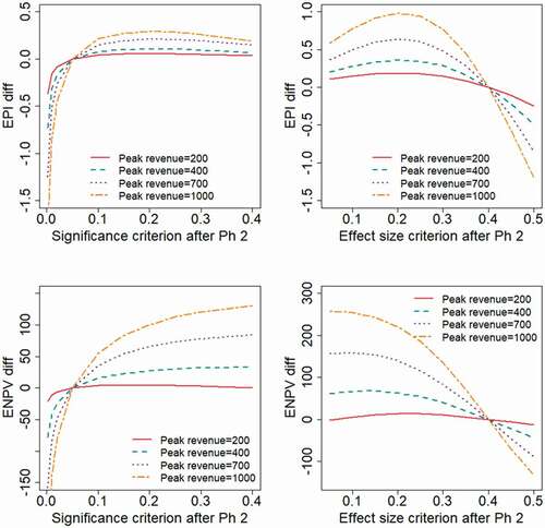
Results obtained when varying the expected peak revenue of the project would illustrate the obvious fact that a reduced sales revenue will lead to lower values for the financial outcome measures. To make the results more interpretable, we have chosen in Figure 5 and 6 to present the outcome measures as differences from the outcomes obtained at reference values for the decision criteria (${\alpha }_2^{crit}=0.05$ and ${\mathrm{\Delta }}_2^{crit}=0.4$, respectively). The results show that with the treatment effect following a log-normal distribution (Figure 5), the EPI is maximized with strict decision criteria (${\alpha }_2^{crit}<0.05$). When the treatment effect has a two-point distribution (Figure 6), more liberal decision criteria will optimize EPI (${\alpha }_2^{crit}$ in the range 0.2–0.25 and ${\mathrm{\Delta }}_2^{crit}\approx 0.2$). If the expected revenue is high, e.g. in the base case where $A_0=700$, the ENPV is generally maximized by adopting high values for ${\alpha }_2^{crit}$, or correspondingly low values for ${\mathrm{\Delta }}_2^{crit}$. With the revenue being sufficiently low (e.g. $A_0=200$) the value of the project is only marginally positive, in which case the decision criterion for a Phase 3 investment decision should be more strict in order to maximize ENPV.

Figure 5. Expected project value as a function of the decision criterion after Phase 2, evaluated for different levels of the peak annual sales revenue, $A_0$. The outcome measures are presented as differences from the values obtained at ${\alpha }_2^{crit}=0.05$ and ${\mathrm{\Delta }}_2^{crit}=0.4$, respectively.

A log-normal distribution is assumed for the treatment effect. Top: Expected Productivity Index (EPI). Bottom: Expected Net Present Value (ENPV).Left: Significance decision criterion, ${\alpha }_2^{crit}$. Right: Effect size decision criterion, ${\mathrm{\Delta }}_2^{crit}$

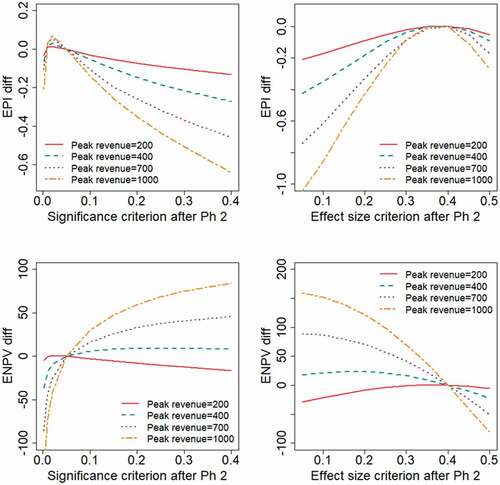
Figure 6. Expected project value as a function of the decision criterion after Phase 2, evaluated for different levels of the peak annual sales revenue, $A_0$. The outcome measures are presented as differences from the values obtained at ${\alpha }_2^{crit}=0.05$ and ${\mathrm{\Delta }}_2^{crit}=0.4$, respectively.

A two-point distribution is assumed for the treatment effect. Top: Expected Productivity Index (EPI). Bottom: Expected Net Present Value (ENPV).Left: Significance decision criterion, ${\alpha }_2^{crit}$. Right: Effect size decision criterion, ${\mathrm{\Delta }}_2^{crit}$

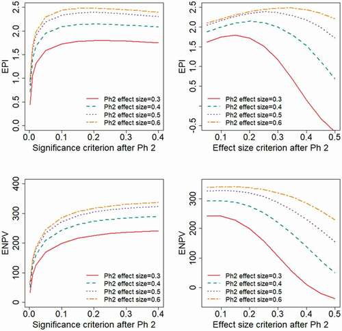
Figures 7 and 8 illustrate the impact if the study design and endpoint available in Phase 2 give different degrees of relative variability, corresponding to different values for the anticipated effect size, ${\mathrm{\Delta }}_2$. The evaluated range of effect size, ${\mathrm{\Delta }}_2=\left\{0.3,0.4,0.5,0.6\right\}$, correspond to the Phase 2 sample size being $N_2=\left\{276,156,100,72\right\}.$ Obviously, both the EPI and ENPV will be higher for scenarios with a higher effect size. In each of the scenarios, the ENPV is maximized by applying a liberal decision criterion (high value of ${\alpha }_2^{crit}$ or low value of ${\mathrm{\Delta }}_2^{crit}$), whereas the appropriate choice of ${\alpha }_2^{crit}$ to maximize EPI will depend on the underlying treatment effect distribution. With a log-normal effect distribution, a strict decision criterion maximizes EPI, choosing ${\alpha }_2^{crit}<0.05$ and ${\mathrm{\Delta }}_2^{crit}\approx {\mathrm{\Delta }}_2$, i.e. the effect size based decision criterion taken to be approximately the effect size anticipated in the planning phase. With a two-point effect distribution, EPI is maximized by choosing ${\alpha }_2^{crit}\approx 0.2$ and ${\mathrm{\Delta }}_2^{crit}\approx {\mathrm{\Delta }}_2/2$, i.e. the effect size based decision criterion taken to be approximately half the effect size anticipated in the planning phase.

Figure 7. Expected project value as a function of the decision criterion after Phase 2, evaluated for different levels of the Phase 2 variability, corresponding to different anticipated effect sizes, ${\mathrm{\Delta }}_2$. The different levels of ${\mathrm{\Delta }}_2$ correspond to the Phase 2 sample sizes: $N_2=\left\{276,156,100,72\right\}$.

A log-normal distribution is assumed for the treatment effect. Top: Expected Productivity Index (EPI). Bottom: Expected Net Present Value (ENPV).Left: Significance decision criterion, ${\alpha }_2^{crit}$. Right: Effect size decision criterion, ${\mathrm{\Delta }}_2^{crit}$

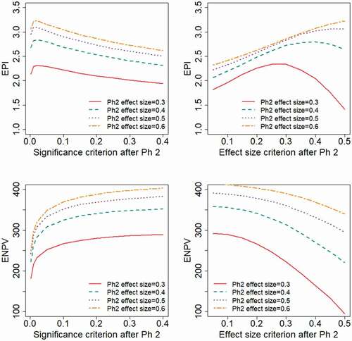
Figure 8. Expected project value as a function of the decision criterion after Phase 2, evaluated for different levels of the Phase 2 variability, corresponding to different anticipated effect sizes, ${\mathrm{\Delta }}_2$. The different levels of ${\mathrm{\Delta }}_2$ correspond to the Phase 2 sample sizes: $N_2=\left\{276,156,100,72\right\}$.

A two-point distribution is assumed for the treatment effect. Top: Expected Productivity Index (EPI). Bottom: Expected Net Present Value (ENPV).Left: Significance decision criterion, ${\alpha }_2^{crit}$. Right: Effect size decision criterion, ${\mathrm{\Delta }}_2^{crit}$

5. Discussion

The net present value is a very commonly used measure whenever financial aspects are brought into quantitative support for decision-making in the pharmaceutical industry. The results of this article may point towards properties of the NPV that makes this measure less appropriate than generally anticipated. Since pharmaceutical development projects often have a very large upside, the NPV tends to be positive even when projects are run at high risk. Consequently, NPV for a portfolio may be maximized by running as many projects as possible, taking a lot of risks and allocating unlimited resources to the development portfolio. This is also reflected in the results of this paper, where liberal decision criteria (high ${\alpha }_2^{crit}$ or low ${\mathrm{\Delta }}_2^{crit}$) are shown to maximize ENPV in many of the scenarios. In reality, however, the available resources are limited, both in terms of the number of projects available for development and in terms of financial resources for funding. Additionally, if the number of projects taken forward to late phase development and to the market would substantially increase, their marginal benefit in terms of efficacy and revenue would likely decrease. Hence, the limited resources need to be focused on those projects that bring the most benefit within available resource limits. The choice of projects, and the design of the projects, should maximize the return on the invested resources and, arguably, measures focusing on the return on investment is therefore better suited for evaluation of drug development strategies. This is also the reason why the EPI outcome measure has been given a prominent place in the results presented in this article. Chen and Beckman (2009) and Chen et al. (2013) used a benefit–cost ratio for their evaluations of Go-NoGo criteria. This measure, being a ratio between benefit and costs, is also a type of return-on-investment indicator and hence has some resemblance to the EPI measure used in this article. While the conclusions from evaluating ENPV consistently indicating liberal decision criteria to be favorable, our results give a more complex picture when decision criteria are based on EPI. With EPI as the outcome measure, the optimal decision criterion is indicated to be context dependent. Aspects like the chosen type II error rate, the related choice of Phase 2 sample size, the anticipated effect size and variability of the Phase 2 endpoint, have all been shown to impact the appropriate choice of decision criterion for maximizing EPI.

We have in this article assumed that the decision criteria, for a successful continuation of a project to the next phase, is based either on statistical significance (i.e. ${\hat{p}}_2<{\alpha }_2^{crit}$) or based on the observed effect size (i.e. ${\hat{\mathrm{\Delta }}}_2>{\mathrm{\Delta }}_2^{crit}$). We are of course aware that other choices of decision criteria may be relevant, and that more elaborate approaches to decision criteria are proposed by some authors, e.g. Frewer et al. (2016). Slightly simplified, their approach involves defining a target value, TV, and a lower reference value, LRV. A ‘Go’ decision is concluded if the observed efficacy is significantly above LRV, and a ‘Stop’ is concluded if a value significantly below TV is observed. The TV of Frewer et al may be represented by the anticipated treatment effect in our model, $E_0$. If we let LRV = 0, the significance-based criterion corresponds to a special case of the Frewer et al criteria. With the sample size and variance assumed in our base case, the decision criterion would be to conclude a ‘Go’ if ${\hat{E}}_2>E_0/2$, with the decision parameter ${\alpha }_2^{crit}\approx 0.2$. While being beyond the scope of this article, it would be an interesting topic of future research to investigate more generally the impact of the decision criteria suggested by Frewer et al, in the context of the development model used in this article.

The development of a new drug is an excessively complex process, and any model used for the analysis of such a process will have to involve simplifications. Although the model used in this article includes many parameters, there are obviously some aspects where the model might be even more elaborate. One such aspect is the relation between the endpoint measured in Phase 2 and 3, respectively. The model applied in this article allows for the Phase 2 endpoint to have less variability (consequently a larger relative effect size), allowing for smaller sample sizes in Phase 2. However, the model assumes that the true effect in Phase 2 is perfectly predictable of the true effect in Phase 3. This assumption may be questioned, as the outcome of a Phase 2 endpoint, based on a surrogate and/or including restrictive inclusion/exclusion criteria, might provide different results than the eventual Phase 3 (and regulatory) endpoint. This non-perfect predictability was in the modelling framework of Wiklund (2019) represented by a between-endpoint correlation. We have in this article implicitly assumed this correlation to be equal to 1. A more thorough assessment of the choice of early efficacy endpoints, and its relation to optimal Go/NoGo criteria for Proof of Concept trials, is provided by Chen et al. (2013). These authors also note that the trial level correlation is more pertinent to Phase III predictability than patient level correlation.

The model for a development project used to obtain the results of this article, includes the assumption of a treatment effect distribution. This represents the fact that, at the time of planning and designing for a project, the true treatment effect is unknown. The assumption of a distribution for the treatment effect resembles the prior distribution in a Bayesian analysis. What distribution to assign is of course not at all obvious. We have chosen to assign a log-normal distribution for the treatment effect, and a background to this choice is found in Wiklund and Burman (2021). These authors extracted studies from the database at www.clinicaltrials.gov, and the underlying effect sizes were deduced. As a comparison, we also produced results using a two-point distribution, in which the drug is either assumed to be void of efficacy or the efficacy equals what is anticipated in the TPP.

The results of this article are based on simulations of a number of scenarios. An alternative might have been to attempt analytical solutions (cf Miller and Burman (2018), Walley and Grieve (2021)). However, an analytical approach requires a rather restrictive model with a limited number of parameters. We have in this article prioritized to obtain results on the basis of a comprehensive model, taking into account various aspects like cost, trial duration, sample sizes, treatment effect distribution, decision criteria, sales revenue, patent expiry etc. The many model parameters are presented in the Appendix. Our belief is that the validity of an extensive and dynamic model, requiring simulations, may in this context provide more relevant (albeit arguably less generalizable) results than analytical results which are necessarily based on less extensive models.

The focus of this article has been to illustrate the impact of choosing different decision criteria for late phase investment decisions. Another obvious question might be to investigate how the trial leading up to the investment decision should be optimally designed. Indirectly, the design question is addressed by evaluating different values of the type II error rate, i.e. corresponding to different sample sizes. It is however a deliberate choice to not focus more on the design and sample size issue. Over the past decades numerous researchers have published thousands of papers on various aspects of clinical trial design. The contribution of this article is instead to shed some light on the less researched area of how to act once the study has been run and decisions need to be taken based on the results.

We have focused the results section of this article on the standard scenario of Phase 2 and Phase 3 development programs. In certain disease areas, e.g. oncology or rare diseases, the situation is often different and less rigorous early phase data are required to proceed to a pivotal trial. A single arm Phase 2 trial, or even a Phase 1b trial with efficacy readouts, may be sufficient to proceed to Phase 3. The approach outlined in the Model section should be useful to evaluate also this situation, with some appropriate adjustment made to the applied decision criteria and with other parameter values assigned for the simulations and numerical results.

As mentioned in the Introduction, much work has been made to address the problem of false positives in Phase 2, and the corresponding risk of costly Phase 3 failures. The proposed remedy for this issue has often been to increase sample size and apply more rigor to investment decisions after Phase 2 (e.g. De Martini 2020; Huang et al. 2019). As we pointed out initially, less focus has been given to the problem of potential false negatives in Phase 2, which might occur if strict decision criteria are applied. We may quote Lindborg et al. (2014) in stating that: “The lost revenue (that is, opportunity cost) stemming from terminating a drug that is in truth effective is typically much greater than the cost of advancing an ineffective molecule into Phase III. Therefore, intuitively it makes sense that the optimum false negative rate should be lower than the optimum false positive rate, as false negative mistakes are more costly. Although this is common sense, it has not been common practice.” Along these lines, the results of this article indicate that the potential risk of false negative decisions might have a substantial negative impact on the expected value of development projects, and that applying liberal decision criteria often increases the value (as measured by ENPV) and sometimes the return of investment (as measured by EPI). The excessively high attrition rates seen in Phase 2, commonly due to inadequate observed efficacy, might to some extent be a reflection of a large number of false negative outcomes. If this is the case, it would represent an inappropriate hampering of the productivity of the pharmaceutical industry. This article does not provide any ultimate answers to these questions, but we argue that the results certainly warrant more research in this area.

Disclosure statement

No potential conflict of interest was reported by the author(s).

Appendix

The parameter values used to define a base case for our model are summarized in Table 1–5. The tables also include comments and, in some cases, information on the rationale or source for the chosen value.

Table 1. Cost and duration parameters of the base case model used in the simulation study

Parameter	Notation	Value	Comment/source
Cost per patient, Phase 2	C2^N	0.05 $M	Estimate taken from Moore et al. (2020)
Fix cost, Phase 2	C2^0	50 $M	Value calibrated to arrive at total Phase 2 cost (60 $M) as given by DiMasi et al. (2016)
Cost per patient, Phase 3	C3^N	0.075 $M
Fix cost, Phase 3	C3^0	200 $M	Value calibrated to arrive at total Phase 3 cost (255 $M) as given by DiMasi et al. (2016)
Recruitment rate, Phase 2	Q2	15	Number of patients enrolled per month
Additional time, Phase 2	T3^0	2 yrs	Value calibrated to arrive at total Phase 2 time (38 months) as given by DiMasi et al. (2016)
Recruitment rate, Phase 3	Q3	50	Number of patients enrolled per month
Additional time, Phase 3	T3^0	2 yrs	Value calibrated to arrive at total Phase 3 time (45 months) as given by DiMasi et al. (2016)
Duration of registration phase	Treg	1.6	Estimate taken from Thomas et al. (2016)
Cost of registration phase	Creg	10

Table 2.

Design and sample size parameters of the base case model used in the simulation study

Parameter	Notation	Value	Comment/source
Sample size, Phase 2	N2	(160)	Approximate number obtained as an average from searching clinicaltrials.gov for all industry sponsored, interventional studies in Phase 2
Sample size, Phase 3	N3	(700)	Approximate number obtained as an average from searching clinicaltrials.gov for all industry sponsored, interventional studies in Phase 3
Anticipated treatment effect size in Phase 2 for sample size calculation	${\mathrm{\Delta }}_2$	0.4	The effect size ${\mathrm{\Delta }}_2=E_0/{\sigma }_2$ is calibrated to give approximately the sample size indicated above. With $E_0=10$ (given on arbitrary scale), the corresponding standard deviation is ${\sigma }_2=25$.
Anticipated treatment effect size in Phase 3 for sample size calculation	${\mathrm{\Delta }}_3$	0.25	The effect size ${\mathrm{\Delta }}_3=E_0/{\sigma }_3$ is calibrated to give approximately the sample size indicated above. With $E_0=10$ (given on arbitrary scale), the corresponding standard deviation is ${\sigma }_3=40$.
Type I error rate used for Phase 2 sample size calculation	α2*	0.1	Assuming 10% level for a two-sided test in Phase 2
Type I error rate used for Phase 3 sample size calculation	α3*	0.05	Assuming 5% level for a two-sided test in Phase 3
Type II error rate used for Phase 2 sample size calculation	β2	0.2	Assuming 80% power is intended for Phase 2
Type II error rate used for Phase 3 sample size calculation	β3	0.1	Assuming 90% power is intended for Phase 3

Table 3.

Treatment effect parameters of the base case model used in the simulation study

Parameter	Notation	Value	Comment/source
Log-normal treatment effect distribution – location parameter	μ2, μ3	1.6	We assume that the true treatment effect distribution is the same for both Phase 2 and Phase 3. The parameters of the treatment effect distribution are chosen to get a probability of launch in the base case (approx. 25%) to be in line with the benchmark data given by Wong et al. (2019).
Log-normal treatment effect distribution – scale parameter	γ2, γ3	1.0
Two-point treatment effect distribution – size of positive efficacy	$E_0$	10	This is the same parameter as used in sample size calculations
Two-point treatment effect distribution – probability of positive efficacy	$p_j$	0.5

Table 4.

Decision criteria parameters of the base case model used in the simulation study

Parameter	Notation	Value	Comment/source
Significance level for successful transition from Phase 2	${\alpha }_2^{crit}$	1%-40%	This is the parameter representing the decision criterion after Phase 2. Outcomes with different values for this parameter are presented in the Results section
Significance level for successful transition from Phase 3	${\alpha }_3^{crit}$	5%	Parameter representing the decision criterion after Phase 3.
Effect size for successful transition from Phase 2	${\mathrm{\Delta }}_2^{crit}$	0.05–0.40	This is the parameter representing the effect-size based decision criterion after Phase 2. Outcomes with different values for this parameter are presented in the Results section
Risk of failure due to non-efficacy reasons (e.g. severe safety finding), Phase 2	π2	10%
Risk of failure due to non-efficacy reasons (e.g. severe safety finding), Phase 3	π3	10%	This approximate number is obtained by combining results from Wong et al. (2019) and Hwang et al. (2016).
Risk of failure in registration phase	πreg	15%	Estimate taken from Thomas et al. (2016) and Hay et al. (2014)

Table 5.

Market parameters of the base case model used in the simulation study

Parameter	Notation	Value	Comment/source
Remaining patent time at start of Phase 2	TP	17
Peak annual sales revenue	A0	700
Discount rate of future cash flows	λ	0.1
Anticipated treatment effect (e.g. in Target Product Profile)	E0	10	This is the same parameter as used in sample size calculations

References

- Chen, C., L. Sun, and C. L. Li. 2013. Evaluation of early efficacy endpoints for proof-of-concept trials. Journal of Biopharmaceutical Statistics 23 (2):413–424. doi:10.1080/10543406.2011.616969.
- Chen, C., and R. A. Beckman. 2009. Optimal cost-effective go-no go decisions in late-stage oncology drug development. Statistics in Biopharmaceutical Research 1 (2):159–169. doi:10.1198/sbr.2009.0027.
- Chuang-Stein, C., and S. Kirby. 2014. The shrinking or disappearing observed treatment effect. Pharmaceutical Statistics 13 (5):277–280. doi:10.1002/pst.1633.
- De Martini, D. 2011. Adapting by calibration the sample size of a phase III trial on the basis of phase II data. Pharmaceutical Statistics 10 (2):89–95. doi:10.1002/pst.410.
- De Martini, D. 2020. Empowering phase II clinical trials to reduce phase III failures. Pharmaceutical Statistics 19 (3):178–186. doi:10.1002/pst.1980.
- DiMasi, J. A., H. G. Grabowski, and R. W. Hansen. 2016. Innovation in the pharmaceutical industry: New estimates of R&D costs. Journal of Health Economics 47:20–33. doi:10.1016/j.jhealeco.2016.01.012.
- FDA, U.S. Food and Drug Administration. 2017. 22 case studies where phase 2 and phase 3 trials had divergent results. https://www.fda.gov/about-fda/reports/22-case-studies-where-phase-2-and-phase-3-trials-had-divergent-results. Source accessed: January 28, 2021.
- Frewer, P., P. Mitchell, C. Watkins, and J. Matcham. 2016. Decision-making in early clinical drug development. Pharmaceutical Statistics 15 (3):255–263. doi:10.1002/pst.1746.
- Gould, A. L., R. Krishna, A. Khan, and J. Saltzman. 2015. Principled structured incorporation of clinical knowledge into strategic development decisions. Therapeutic Innovation & Regulatory Science 49 (2):289–296. doi:10.1177/2168479014558273.
- Hay, M., D. W. Thomas, J. L. Craighead, C. Economides, and J. Rosenthal. 2014. Clinical development success rates for investigational drugs. Nature Biotechnology 32 (1):40–51. doi:10.1038/nbt.2786.
- Huang, B., E. Talukdera, L. Hanb, and P. F. Kuanc. 2019. Quantitative decision-making in randomized Phase II studies with a time-to-event endpoint. Journal of Biopharmaceutical Statistics 29 (1):189–202. doi:10.1080/10543406.2018.1489400.
- Hwang, T. J., D. Carpenter, J. C. Lauffenburger, B. Wang, J. M. Franklin, and A. S. Kesselheim. 2016. Failure of investigational drugs in late-stage clinical development and publication of trial results. JAMA Internal Medicine 176 (12):1826–1833. doi:10.1001/jamainternmed.2016.6008.
- Ioannidis, J. P. A. 2005. Contradicted and initially stronger effects in highly cited clinical research. Journal of the American Medical Association 294 (2):218–228. doi:10.1001/jama.294.2.218.
- Kirby, S., J. Burke, C. Chuang-Stein, and C. Sin. 2012. Discounting phase 2 results when planning phase 3 clinical trials. Pharmaceutical Statistics 11 (5):373–385. doi:10.1002/pst.1521.
- Lennie, J. L., J. T. Mondick, and M. R. Gastonguay. 2021. Bayesian modeling and simulation to inform rare disease drug development early decision-making: Application to Duchenne muscular dystrophy. bioRxiv Preprint. doi:10.1101/2021.02.05.429907.
- Lindborg, S., C. Persinger, A. Sashegyi, C. Mallinckrodt, S. J. Ruberg, et al. 2014. Statistical refocusing in the design of Phase II trials offers promise of increased R&D productivity. Nature reviews. Drug discovery 13 (8):638–640. doi:10.1038/nrd3681-c1.
- Miller, F., and C. F. Burman. 2018. A decision theoretical modeling for Phase III investments and drug licensing. Journal of Biopharmaceutical Statistics 28 (4):698–721. doi:10.1080/10543406.2017.1377729.
- Moore, T. J., J. Heyward, G. Anderson, and G. C. Alexander. 2020. Variation in the estimated costs of pivotal clinical benefit trials supporting the US approval of new therapeutic agents, 2015–2017: A cross-sectional study. BMJ Open 10 (6):e038863. doi:10.1136/bmjopen-2020-038863.
- Mudge, J. F., L. F. Baker, C. B. Edge, and J. E. Houlahan. 2012. Setting an Optimal □ That Minimizes Errors in Null Hypothesis Significance Tests. PLoS ONE 7 (2):e32734. doi:10.1371/journal.pone.0032734.
- Pereira, T. V., R. I. Horwitz, and J. P. A. Ioannidis. 2012. Empirical evaluation of very large treatment effects of medical interventions. JAMA 308 (16):1676. doi:10.1001/jama.2012.13444.
- Thomas, D. W., J. Burns, J. Audette, A. Carroll, C. Dow-Hygelund, and M. Hay. 2016. Clinical Development Success Rates 2006-2015. BIO Industry Analysis. https://www.bio.org/sites/default/files/legacy/bioorg/docs/Clinical%20Development%20Success%20Rates%202006-2015%20-%20BIO,%20Biomedtracker,%20Amplion%202016.pdf
- Walley, R. J., and A. P. Grieve. 2021. Optimising the trade-off between type I and II error rates in the Bayesian context. Pharmaceutical Statistics 2021:1–11. https://doi.org/10.1002/pst.2102.
- Wiklund, S. J. 2019. A modelling framework for improved design and decision-making in drug development. PLoS ONE 14 (8):e0220812. doi:10.1371/journal.pone.0220812.
- Wiklund, S. J., and C. F. Burman. 2021. Selection bias, investment decisions and treatment effect distributions. Pharmaceutical Statistics 2021:1–15. doi:10.1002/pst.2132.
- Wong, C. H., K. W. Siah, and A. W. Lo. 2019. Estimation of clinical trial success rates and related parameters. Biostatistics 20 (2):273–286. doi:10.1093/biostatistics/kxx069.