Survival stacking with multiple data types using pseudo-observation-based-AUC loss

ABSTRACT

There have been many strategies to adapt machine learning algorithms to account for right censored observations in survival data in order to build more accurate risk prediction models. These adaptions have included pre-processing steps such as pseudo-observation transformation of the survival outcome or inverse probability of censoring weighted (IPCW) bootstrapping of the observed binary indicator of an event prior to a time point of interest. These pre-processing steps allow existing or newly developed machine learning methods, which were not specifically developed with time-to-event data in mind, to be applied to right censored survival data for predicting the risk of experiencing an event. Stacking or ensemble methods can improve on risk predictions, but in general, the combination of pseudo-observation-based algorithms, IPCW bootstrapping, IPC weighting of the methods directly, and methods developed specifically for survival has not been considered in the same ensemble. In this paper, we propose an ensemble procedure based on the area under the pseudo-observation-based-time-dependent ROC curve to optimally stack predictions from any survival or survival adapted algorithm. The real application results show that our proposed method can improve on single survival based methods such as survival random forest or on other strategies that use a pre-processing step such as inverse probability of censoring weighted bagging or pseudo-observations alone.

KEYWORDS:

• Pseudo-observations
• pseudo-observation-based AUC
• inverse probability of censoring weighting
• survival machine learning
• stacking

1. Introduction

Supervised machine learning (ML) algorithms that target a particular outcome are now a standard tool available for building risk prediction models (Ambale-Venkatesh et al. 2017; Corey et al. 2018; Gulshan et al. 2016; Weng et al. 2017). Particularly when the risk under consideration is that of death, censoring due to the end of follow-up or dropout from a cohort or observational study can complicate the analysis of the value of interest, the risk of an event occurring prior to a given time point. Although many standard methods exist for performing inference on right censored data, such as Cox proportional hazards regression or parametric survival models (Cox 1972), they are not as flexible as ML methods, and fewer machine learning methods that can accommodate right censored data have been developed in comparison to methods for classification. Ensemble methods like bagging, boosting, and stacking that combine predictions from several machine learning algorithms can provide additional improvements in predictive accuracy, but this requires a greater number of ML methods and classes of methods that account for right censoring.

In comparison to 10 years ago, there are now a large number of ML methods that allow for the use of right censored data for the goal of risk prediction via supervised learning. However, most methods have been adaptations of specific ML algorithms or models or within specific classes of methods, such as the adaptation of trees to survival-based trees and survival random forests (Ishwaran et al. 2014, 2008), which are ensemble of trees. In addition, there have also recently been some pre-processing methods proposed using inverse probability of censoring weighted bootstrapping, called IPCW bagging, which allows for the adaption of all classification ML methods to right censored and competing risks data to predict the risk of an event prior to some fixed time (Gonzalez Ginestet et al. 2020). Sachs et al. (2019) proposed the use of pseudo-observations as the outcome of stacked ensembles of ML methods for continuous outcomes, as pseudo-observations are continuous. Both of these pre-processing methods allow for a large number of ML methods to be used in right censored data, without ignoring censored observations.

However, even the pre-processing methods suggested in Gonzalez Ginestet et al. (2020) and Sachs et al. (2019), as well as the single algorithm methods (Ishwaran et al. 2014, 2008), are limited to the class of algorithms or outcome types. When using right censored survival outcomes, this may limit the available predictive methods. Each algorithm may have its own merits and estimation methods, yet in practice, it is not possible to know which algorithm should perform best on a given dataset. Said another way, for each ML algorithm that is theoretically justified and shown to work well practically, there exists a dataset in which it will perform poorly. Thus, we propose to allow for ensembles of standard survival methods such as Cox and parametric survival models, inverse probability of censoring weighted (IPCW) binary outcome methods, including methods that allow weighting or those using the IPCW bagging methods of Gonzalez Ginestet et al. (2020) or simple binary methods ignoring censoring, as well as pseudo-observation based methods all in the same stack. We propose to optimally stack these methods using as the loss function the pseudo-observation-based-AUC, which allows for the use of all data, censored or not, and the responses from all ML methods to be stacked.

We find that by including multiple ML types, which consider the survival outcome in different ways, we can improve upon even the stacked methods that use only one ML algorithm type or type of outcome, such as those for binary or continuous outcomes alone. We demonstrate this using two breast cancer datasets: one from the survival package (Therneau 2020; Therneau and Grambsch 2000) in R (R Core Team 2020) and the other from the Molecular Taxonomy of Breast Cancer International Consortium (METABRIC) (Curtis et al. 2012). In Section 2, we outline our notation and method before demonstrating it in the breast cancer datasets, in Section 3. Finally, Section 4 outlines the limitations of our method and suggests some possible areas of future research.

2. Method

2.1. Notation and preliminaries

Let $Y_i$ be the right censored event time, $T_i$ be the true event time, and ${\mathrm{\Delta }}_i\in \{0,1\}$ be the event indicator where 0 indicates censoring and 1 indicates failure, for subjects $i=1,\dots ,n$. Let ${\mathbf{X}}_{\mathbf{i}}=(X_{i1},\dots X_{ip})$ denotes the vector of covariates for subject $i$ where $X_{ij}$ denotes the biomarker measurement $j$ (or covariate $j$) measured at baseline for subject $i$. We assume that the censoring time is independent of the failure-event time and the covariates.

We are interested in predicting the risk of failure within $t$ time units for subject $i$. This quantity corresponds to the cumulative incidence of failure up to time $t$:

$C(t)=E\{I(T\le t)\}=P\{T\le t\}.$

We summarize the survival data as the counting process: $N(t)={\sum }_{i}I(Y_i\le t,{\mathrm{\Delta }}_i=1),$ giving the number of observed failures on or before time $t$, and $R(t)={\sum }_{i}I(Y_i\ge t)$ gives the number of subjects still at risk just before time $t$. Our estimator of the marginal quantity $C(t)$ of the cumulative incidence function is the Aalen-Johansen estimator (Aalen and Johansen 1978) $\hat{C}(t)={\int }_0^t\hat{S}(u)d\hat{A}(u),$ where $\hat{A}(t)={\int }_0^{t}dN(u)/R(u)$ is the Nelson-Aalen estimator for the cumulative hazard for failures, and $\hat{S}$ is the Kaplan–Meier estimator of the overall survival. This is equivalent to one minus the Kaplan–Meier estimator of the survivor function, but the theoretical development was done to accommodate competing risks (Graw et al. 2009), which we do not consider here.

The goal then is to predict an individual’s risk based on their covariate vector ${\mathbf{X}}_{\mathbf{i}}$ by flexibly fitting a model for

$P\{T_i\le t|{\mathbf{X}}_{\mathbf{i}}={\mathbf{x}}_{\mathbf{i}}\}=f({\mathbf{x}}_i),$

where $f$ denotes a generic prediction function that takes as input the observed covariate vector and which may also depend on some parameters. For example, $f$ may represent a parametric regression model, a tree-based model, or the result of a $k$ nearest neighbor algorithm. We let $\hat{f}$ denote the estimated prediction function, and we will distinguish between prediction functions estimated by different algorithms or on different subsets of the data using subscripts.

2.2. Cross-validation of prediction functions

Consider a set of $K$ prediction algorithms, which we will call the library of prediction algorithms. In general, a prediction algorithm with index $k$ for $k=1,\dots ,K$, could be any method that takes training data (including the outcome and covariates) as input, and outputs a prediction function ${\hat{f}}_k$. For example, regression methods, penalized regression methods, tree-based methods, and nearest neighbor methods, to name a few. This library of methods should be pre-specified by the analyst, and our key contribution is that the library may contain a mix of IPCW classification, pseudo-observation based regression, and survival-specific methods. Each method may require pre-processing of the censored time-to-event outcome, estimation of weights, or specification of tuning parameters.

We proceed by constructing an $n\times K$ matrix $\mathbf{Z}$ of cross-validated or “pre-validated” (Tibshirani and Efron 2002) predictions for each subject and of the prediction algorithms under consideration as follows. Split the dataset into a partition, according to a $V$-fold cross validation scheme: split the $n$ observations into $V$ approximately equal size groups. Let the $\nu$-th group be the validation sample, and the remaining group the training sample, $\nu =1,\dots ,V$. Define $\mathcal{X}$ to be the full dataset, $V(\nu )$ to be the $\nu$ th validation data split, $T(\nu )=\mathcal{X}\mathrm{\setminus }V(\nu )$ to be the $\nu$ th training data split for $\nu =1,\dots ,V$.

1. For $\nu \in 1,\dots ,V$:

 (a) For $k\in 1,\dots ,K$:

i. Estimate the model ${\hat{f}}_{\nu ,k}$ using $T(\nu )$ and the algorithm $k$ from the library.

ii. Output predictions ${\hat{f}}_{\nu ,k}(V(\nu ))=Z_{\nu ,k}$ into the $k$ th column and appropriate rows of $\mathbf{Z}$.

Each algorithm in the library can use whichever estimation method is appropriate for that type of model. For instance, a typical choice for survival data would be a Cox model (Cox 1972), in which case the algorithm would maximize the partial likelihood. Another sensible option, given that we are trying to predict the risk at time $t$, is to use pseudo-observation regression for the cumulative incidence at that time point (Andersen and Pohar Perme 2010). Next, we will create an ensemble over $\mathbf{Z}$ by optimizing a loss function that targets our prediction quantity of interest. Specifically, we will seek to find a coefficient vector $\alpha$ (a column vector of length $K$) such that $\mathbf{Z}\alpha$ is optimal in the sense that it optimizes our loss function of interest.

2.3. AUC loss using pseudo-observations

Following Andersen and Pohar Perme (2010), the $i$ th pseudo-observation time $t$ is defined as

${\hat{C}}^i(t)=n\hat{C}(t)-(n-1){\hat{C}}^{-i}(t),$

where ${\hat{C}}^{-i}(t)$ is the Aalen–Johansen estimate of the cumulative incidence function that is computed by using the sample excluding the $i$ th observation from the full sample of size $n$. By construction and the unbiasedness of the Aalen–Johansen estimator, the pseudo-observations are unbiased for the cumulative incidence: $E\{{\hat{C}}^i(t)\}=C(t).$ Moreover, observe that the survival can be related to the pseudo-observations by $E\{1-{\hat{C}}^i(t)\}=P(Y_i>t)$.

An important property of pseudo-observations that we will exploit is asymptotic unbiasedness conditional on covariates, i.e.,

(1) $E({\hat{C}}^i(t)|{\mathbf{X}}_i={\mathbf{x}}_i)=P(T_i\le t|X_i={\mathbf{x}}_i)+o_p$(1)

in large samples. Graw et al. (2009) proved that (1) holds for the Aalen-Johansen estimator when the censoring is independent of the event time and of all covariates in the model. This can be relaxed by using inverse probability of censoring weighted estimators instead of the Aalen–Johansen (Binder and Schumacher 2008).

For some coefficient vector $\alpha$, let $B_i=Z_i^{\mathrm{T}}\alpha$ denotes the ensemble predicted outcome for subject $i$ and let $c_1,\dots ,c_m$ denote the unique values or a fixed grid of the $B_i$ values sorted in descending order. Then, the time dependent AUC at time $t$ for failure, calculated by the trapezoidal rule, can be written as

$\widehat{AUC}(t)=\sum _{j=1}^{m-1}0.5(x_{j+1}-x_j)(y_{j+1}+y_j),$

where

$y_j=\frac{{\sum }_{i=1}^n{C}^i(t)\varphi (B_i,c_j)}{{\sum }_{i=1}^n{C}^i(t)}$

and

$x_j=\frac{{\sum }_{i=1}^n(1-C^i(t))\varphi (B_i,c_j)}{{\sum }_{i=1}^{n}1-C^i(t)},$

where $\varphi$ is a ramp function. A ramp function in this context measures to what degree the first argument is greater than the second argument. One example is the indicator step function: ${\varphi }^{\ast }(a,b)=1$ if $a>b$ and is 0 otherwise, which yields the empirical AUC. To see this relationship to the receiver operating characteristic (ROC) curve, note that the numerator of $y_j$ is an estimate of

(1) $E\left\{\frac{1}{n}\sum _n^{i=1}{C}^i(t)I(B_i>c_j)\right\}=P(T_i\le t,B_i>c_j)+o_p$(1)

and the denominator is an estimate of $P(T_i\le t_{\star })$. Since the numerator and the denominator are asymptotically unbiased under conditions (A1) and (A2) of (Graw et al. 2009) which state that the censoring time is stochastically independent of the event time, the event indicator and the covariates, and that the time point of interest are chosen such that the probability of remaining uncensored is bounded away from 0 at that time point, by the continuous mapping theorem, their ratio is a reasonable estimator of $P(B_i>c_j|T_i\le t)$, which is the time-dependent true positive fraction (Heagerty et al. 2000) at $c_j$. Similarly, $x_j$ is an estimator of the time-dependent false positive fraction at $c_j$. These two quantities estimated at all $c_1,\dots ,c_m$ yield the ROC curve, and the trapezoidal rule calculates the area under it.

Since our goal is to find the $\alpha$ that maximizes the AUC, the step ramp function is not ideal as it includes non-differentiable points. Instead, we use a smoothed ramp function as suggested by Fong et al. (2016), the sigmoid ramp:

$\varphi (a,b;\sigma )=\frac{1}{1+exp((b-a)/\sigma )},$

for a fixed, small value of $\sigma$. We set the parameter $\sigma$ equal to $0.01$ in our data analysis. See Fong et al. (2016) for other ways to select this parameter.

Our goal is to optimize $\widehat{AUC}(\alpha ,t)$ with respect to $\alpha$ for a fixed $t$. Maximization of the AUC is difficult, in general, because the ROC curve is invariant to monotone transformations of the predictor, regardless of how the ROC curve is estimated (Fong et al. 2016; Pepe 2000). Multiplication of the coefficient vector by a constant does not change the AUC and hence, without any restrictions, the solution $\hat{\alpha }$ is not unique. Adding a penalty term to the objective function, denoted by $\lambda$, is one way to solve this problem and obtain a unique solution for $\alpha$. Following Fong et al. (2016), we select the normalized vector ${\alpha }^{\ast }=\frac{\alpha }{{\sum }_{k=1}^K{\alpha }_k}$ such that

$\underset{{\alpha }^{\ast }>0}{max}\left\{\widehat{AUC}({\alpha }^{\ast },t)-\lambda \sum _k|{\alpha }_k^{\ast }{|}^2\right\}.$

Using the smooth ramp function, the gradient of this objective with respect to $\alpha$ exists at all points, which will give us better optimization properties. Regardless of how the predictors in $\mathbf{Z}$ are created, this ensemble technique will ensure that the final product targets the quantity of interest and will borrow strength from the different algorithms in a data-driven manner. It has been suggested to normalize the coefficients by their sum and to restrict coefficients to being greater than zero to improve calibration. Although this is clearly useful when the predictions from the individual ML methods are all probabilities, when the predictions are pseudo-observation based or simply the linear predictor from a Cox model it is less clear what, if any, advantages this offers. In our example, we found that restricting coefficients to be greater than zero improved performance slightly in cross-validation. This can therefore be considered something to optimize a further tuning parameter of the stacking procedure.

2.4. Creating the final ensemble predictor and evaluating performance

For $k=1,\dots ,K$, fit each algorithm on the full dataset to obtain ${\hat{f}}_k({\mathbf{X}}_i,t)$, for $i=1,\dots ,n$. This forms an $n$ by $K$ matrix where the rows are predicted outcomes for each subject, and the columns correspond to different prediction methods. The final predictor is the linear combination ${\alpha }^{\ast \mathrm{T}}{\hat{f}}_k$ according to the optimized coefficient vector $\hat{\alpha }$ obtained in the previous step. This also gives us the final prediction function $\hat{f}$ that can be applied to new observations.

It is recommended to comprehensively evaluate the performance of this predictor in an independent validation sample, including discrimination, calibration, and measures of explained variation (Royston and Altman 2013; Steyerberg et al. 2010). In our illustrative examples, as a measure of discrimination, we report the time dependent receiver operating characteristic curve (Heagerty et al. 2000) where the true and false positive fractions are estimates as detailed above. Additionally, we construct a predictiveness curve (Pepe et al. 2007) for the risk outcome using smooth regression of the pseudo-observations conditional on the predicted risk for calibration. The fitted values from this model provide an estimate of the predictiveness curve (Sachs et al. 2019). Specifically, the function

$E[C^i(t)|\hat{f}({\mathbf{X}}_i)=x]$

is specified as a generalized additive model (Hastie and Tibshirani 1990) as an estimate of the conditional risk

$P(T_i\le t|\hat{f}({\mathbf{X}}_{\mathbf{i}})=x).$

This estimation procedure works for the same reason that pseudo-observation regression does, namely, that conditional means of pseudo-observations are asymptotically unbiased (Graw et al. 2009).

Finally, measures of explained variation and associations between the predicted risk and the observed outcome are estimated using the explained variation statistic described by Royston and Sauerbrei (2004), by fitting Cox regression models with continuous and categorized risk as the predictors, and the Kaplan–Meier curves stratified by the categorized risk, as recommended by Royston and Altman (2013).

3. Illustrative examples

We illustrate our proposed method using the two breast cancer datasets: the ones used in Royston and Altman (2013) (Royston–Altman) and the Molecular Taxonomy of Breast Cancer International Consortium (METABRIC) (Curtis et al. 2012).

3.1. Royston–Altman dataset

Following Royston and Altman (2013), we used the Rotterdam data as our training data and the German Breast Cancer Study Group (GBSG) as our external validation set. These dataset are available in the survival package (Therneau 2020; Therneau and Grambsch 2000) in R (R Core Team 2020) under the name Rotterdam and GBSG, respectively. The Rotterdam tumor bank includes 2982 primary breast cancers patients. Following Royston and Altman (2013), we restrict to the 1546 node positive patients because the validation data includes only node positive patients. However, we do not use the same outcome or target of prediction. We consider the outcome of progression or death within 5 years of primary surgery, rather than the outcome of risk of recurrence or death at anytime, nor do we limit the follow-up of patients included in the data, as was done in Royston and Altman (2013).

The GBSG validation data contain 720 patients with primary node positive breast cancer who were enrolled in a clinical trial from July 1984 to December 1989, see Schumacher et al. (1994) for more detail. The maximum follow-up time available was 7 years. We used the same prognostic factors that in Royston and Altman (2013): age in years at primary surgery, menopausal status, tumour size, number of positive lymph nodes, progesterone receptors, oestrogen receptors, and hormonal treatment. Just as in Royston and Altman (2013), we categorized tumor size as $\le$ 20 mm, between 20 to 50 mm and $>$ 50 mm. All methods run on these data used all covariates. Based on the model build in the Rotterdam data, we predict death or recurrence within 5 years of primary surgery in the GBSG data as a validation of the model.

4. Metabric

METABRIC database is a Canada-UK project which contains targeted sequencing data of breast cancer samples. METABRIC cohort were collected between 1977 and 2005 from five centers in the UK and Canada (Curtis et al. 2012; Mukherjee et al. 2018). The clinical data were downloaded from cBioportal (http://www.cbioportal.org) on October 2021 and contains 1904 patients. We considered the following prognostic factors: age at diagnosis, menopausal status, tumour size, number of positive lymph nodes examined, tumor grade, progesterone and oestrogen receptors status, hormonal and radiotherapy treatment, and the Nottingham prognostic index (NPI). The number of positive lymph nodes examined was categorized as greater than and equal to 0. The only continuous variables are age at diagnosis, tumor size, and NPI. The rest of the variables are binary. All methods run on these data used all covariates. We split the patients randomly into training (70%) and validation (30%) set, respectively. We considered two endpoints: overall survival (OS) and recurrence-free survival (RFS) in months. Based on the model build in the training data, we predict the risk of dying and of breast cancer recurrence within 5 years in the validation dataset.

5. Results

To generate predictions, we fit Cox regression with stepwise selection, a survival random forest (Ishwaran et al. 2008), and a Cox Boost model (Binder et al. 2009). These are our survival based methods of comparison. We also fit a inverse probability of censoring weighted (IPCW) logistic regression and an IPCW bagged support vector machine and an IPCW bagged k-nearest neighbors (KNN) algorithm for the binary outcome of observed death or recurrence within 5 years. The IPCW and the IPCW bagging are implemented as outlined in Gonzalez Ginestet et al. (2020). These three methods serve as our comparators in the classification class of ML methods. Finally, we fit pseudo-observation based linear models, applying a LASSO penalty (Friedman et al. 2010), and non-penalized GLM models using an identity link for five different time-points separately (Sachs and Gabriel 2021). We denote these models as LASSO eventglm and eventglm, respectively. In each of these 10 models, we also included B-splines with three knots for all continuous predictors. We used the grid of time points $\{2,4,5,6,7\}$ years for Royston–Altman dataset and a grid of time points $\{3,4,5,6,7\}$ years for the METABRIC dataset. We selected appropriate tuning parameters, when needed, via internal cross-validation. The specification for each method as well as the code for reproducing our results can be found at https://github.com/pablogonzalezginestet/megalearner.

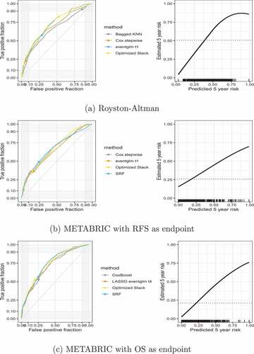
We additionally combine all methods into a single ensemble using 10-fold cross-validation and the pseudo-observation-based-AUC loss function at 5 years for a linear function of the predictions of each method. The results in the validation set for each respective dataset are illustrated in Table 1. As can be seen in Table 1, the optimized stack AUC for the 5 year risk in the validation sample in the GBSG and METABRIC using the OS is 0.718 and 0.745, respectively. Both are superior to all other individual methods, with one exception: in the validation sample of the METABRIC using the RFS, the optimized stack AUC performed similarly to best individual method, which is LASSO eventglm at $t_5$.

Table 1. Summary of the models used in the ensemble. AUC column is the validation sample AUC for the individual model at 5 years and the normalized coefficient is the estimated ${\alpha }^{\ast }$. METABRIC ${ }_{RFS}$ and METABRIC ${ }_{OS}$ refer to the analysis that uses recurrence-free survival and overall survival as endpoints in the dataset METABRIC, respectively. SRF refers to survival random forests. The grid of time points $t_1,\dots ,t_5$ is $\{2,4,5,6,7\}$ years for Royston–Altman and $\{3,4,5,6,7\}$ years for METABRIC.

	Royston–Altman		METABRIC ${ }_{RFS}$		METABRIC ${ }_{OS}$
Method (R package)	AUC	${\alpha }^{\ast }$	AUC	${\alpha }^{\ast }$	AUC	${\alpha }^{\ast }$
Cox stepwise (survival)	0.697	0.001	0.667	0.001	0.721	0.001
SRF (randomForestSRC)	0.685	0.001	0.671	0.132	0.739	0.207
CoxBoost (CoxBoost)	0.697	0.045	0.675	0.218	0.718	0.033
IPCW Logistic stepwise (stats)	0.707	0.009	0.662	0.001	0.741	0.052
Bagged SVM (e1071)	0.702	0.001	0.621	0.086	0.720	0.001
Bagged KNN (class)	0.653	0.062	0.622	0.039	0.678	0.030
eventglm at $t_1$ (eventglm)	0.713	0.262	0.648	0.510	0.718	0.157
eventglm at $t_2$ (eventglm	0.709	0.122	0.658	0.001	0.732	0.205
eventglm at $t_3$ (eventglm)	0.712	0.054	0.663	0.001	0.741	0.001
eventglm at $t_4$ (eventglm)	0.707	0.052	0.670	0.001	0.742	0.081
eventglm at $t_5$ (eventglm)	0.703	0.097	0.676	0.001	0.742	0.155
LASSO eventglm at $t_1$ (glmnet)	0.705	0.107	0.634	0.001	0.638	0.001
LASSO eventglm at $t_2$ (glmnet)	0.695	0.162	0.649	0.001	0.672	0.049
LASSO eventglm at $t_3$ (glmnet)	0.685	0.006	0.660	0.001	0.713	0.001
LASSO eventglm at $t_4$ (glmnet)	0.660	0.019	0.675	0.001	0.721	0.001
LASSO eventglm at $t_5$ (glmnet)	0.661	0.003	0.688	0.001	0.738	0.025
Optimized stack	0.718		0.674		0.745

Although it may seem counterintuitive, the pseudo-observation-based AUC at 5 years is not always highest for the pseudo-observation based methods. Furthermore, it will not always be the case that pseudo-observation-based methods will seem to have superior performance to other outcome based methods, as can be seen by comparing the glmnet pseudo-observation-based methods to the IPCW Logistic stepwise method.

Figure 1 depicts the ROC curve and the predictiveness curve for the optimized stack method for the 5 year risk. For visual representation, the ROC curve for the optimized stack is displayed with three individual methods that were chosen depending on its contribution to the final model. We chose the individual methods that resulted in having the largest contribution and one that had a modest contribution and one that had practically no contribution. We also displayed in the ROC curve the risk threshold at or above 0.30 for each method. In the Royston–Altman example, the optimized stack had a 0.825 sensitivity and 0.474 specificity at 0.30 risk threshold. In the METABRIC dataset, the optimized stack had a lower sensitivity (0.520 and 0.373 in the OS and RFS as endpoints respectively) but higher specificity (0.803 and 0.851 in the OS and RFS as endpoints, respectively). Since the ROC curves did not align by risk thresholds, they do not allow direct comparison by thresholds.

Figure 1. ROC curve (left panel) and estimated predictiveness curves (right panel) for the optimal ensemble in the validation data. The dots show the risk threshold at or above 0.30 (left panel). The right panels show the predicted 5-year risk as output from the ensemble (x-axis) versus the estimated 5-year risk conditional on the predicted (y-axis). The conditional estimated risk is based on the locally weighted smoothed average of the pseudo-observations, the dotted line is the marginal risk based on the unconditional average of the pseudo-observations, and the bottom black dashes are the rug showing the distribution of the predicted values.

Figure 2 depicts the KM curves for the predicted risk categorized into quartiles for each example. The example of Royston–Altman demonstrated good discrimination over the entire time range. Instead, METABRIC’s example did not show good separation between the second (Q2) and third quartile (Q3), particularly the example with RFS as endpoint. This can also be seen in Table 2 that shows the survival estimates in addition to the number of events and number of individuals at risk per each time point corresponding to Figure 2.

Table 2. Number at risk (#risk), number of events (#events), survival probability (Surv), and 95% confidence interval (CI) for four time points (T) of the Kaplan–Meier estimates of survival probabilities in the validation data grouped by risk quartiles (Q1, Q2, Q3, and Q4) corresponding to Figure 2.

Statistic	Royston–Altman	METABRIC ${ }_{RFS}$	METABRIC ${ }_{OS}$
AUC 5-years	0.718 (0.024)	0.672 (0.027)	0.745 (0.025)
Survival concordance	0.687 (0.018)	0.630 (0.021)	0.672 (0.02)
Explained variation	0.198 (0.031)	0.088 (0.032)	0.142 (0.034)
HR per 0.1 units	1.455 (0.034)	1.184 (0.027)	1.298 (0.030)
HR Q2 vs Q1	2.004 (0.203)	1.530 (0.214)	2.213 (0.183)
HR Q3 vs Q1	2.977 (0.197)	1.600 (0.212)	2.399 (0.183)
HR Q4 vs Q1	5.481 (0.190)	2.624 (0.200)	4.012 (0.179)

Figure 2. Kaplan–Meier estimates of survival probabilities in the validation data grouped by quartiles of the risk score. Solid lines are survival curves and dashed lines represent 95% confidence interval.

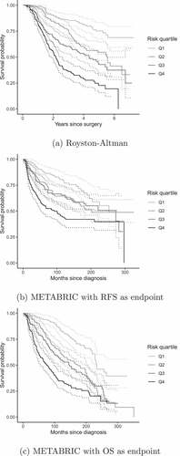
Finally, Table 3 shows discrimination measures and hazard ratios evaluated in the validation datasets that complement the information shown in the KM curves. Royston–Altman’s example showed better discrimination performance than both METABRIC’s examples: hazard ratios were more separated between risk groups and it had larger survival concordance and explained variation. As we discussed in the KM curves, the poor discrimination between Q2 and Q3 in METABRIC is reflected in a close hazard ratio between these two risk groups.

Table 3. Measures of performance and discrimination in the validation dataset. Standard errors were computed using 200 bootstrap replicates and are shown between round brackets. HR = hazard ratio; Q = quartile.

Royston–Altman
Q1					Q2
T	#risk	#events	Surv	95% CI	T	#risk	#event	Surv	95% CI
0	172	0	1.00	(1.00–1.00)	0	171	0	1.00	(1.00–1.00)
2	141	16	0.90	(0.85–0.95)	2	128	25	0.84	(0.79–0.90)
4	89	12	0.81	(0.75–0.88)	4	61	31	0.60	(0.52–0.69)
6	17	8	0.69	(0.59–0.79)	6	9	9	0.42	(0.31–0.56)
Q3					Q4
0	171	0	1.00	(1.00–1.00)	0	172	0	1.00	(1.00–1.00)
2	105	50	0.69	(0.63–0.77)	2	85	74	0.55	(0.48–0.63)
4	55	22	0.53	(0.45–0.62)	4	24	33	0.29	(0.22–0.38)
6	9	11	0.37	(0.28–0.49)	6	1	5	0.19	(0.12–0.31)
METABRIC with RFS as endpoint
Q1					Q2
T	#risk	#events	Surv	95% CI	T	#risk	#event	Surv	95% CI
0	137	1	0.99	(0.98–1.00)	0	136	0	1.00	(1.00–1.00)
100	82	21	0.83	(0.76–0.90)	100	66	43	0.64	(0.56–0.74)
200	20	12	0.62	(0.51–0.75)	200	22	9	0.51	(0.42–0.63)
Q3					Q4
0	136	0	1.00	(1.00–1.00)	0	136	0	1.00	(1.00–1.00)
100	68	43	0.66	(0.59–0.75)	100	54	65	0.50	(0.42–0.59)
200	21	8	0.55	(0.46–0.66)	200	20	8	0.42	(0.34–0.52)
METABRIC with OS as endpoint
Q1					Q2
T	#risk	#events	Surv	95% CI	T	#risk	#event	Surv	95% CI
0	137	1	0.99	(0.98–1.00)	0	136	0	1.00	(1.00–1.00)
100	82	21	0.83	(0.76–0.90)	100	66	43	0.64	(0.56–0.74)
200	20	12	0.62	(0.51–0.75)	200	22	9	0.51	(0.42–0.63)
Q3					Q4
0	136	0	1.00	(1.00–1.00)	0	136	0	1.00	(1.00–1.00)
100	68	43	0.66	(0.59–0.75)	100	54	65	0.50	(0.42–0.59)
200	21	8	0.55	(0.46–0.66)	200	20	8	0.42	(0.34–0.52)

6. Discussion

We have demonstrated that the pseudo-observation-based AUC can be used to optimize a survival-based stack of predictions from ML methods using various survival outcomes or methods to account for right censoring. We have illustrated our proposed method by re-analyzing the datasets used in Royston and Altman (2013), the Rotterdam as training data and German Breast Cancer Study Group (GBSG) as an external validation set, and also analyzing data from the METABRIC study using two different outcomes (Curtis et al. 2012; Mukherjee et al. 2018). Based on these two real datasets, we have shown that our proposed method can improve, marginally, the performance of predictions based on a single ML method, for instance, survival random forest (Ishwaran et al. 2008), or a classical survival methods such as Cox proportional hazard model. Our approach seems to be a better alternative to methods that only use ensembles of the same class of ML methods such as IPCW Bagging for binary outcomes (Gonzalez Ginestet et al. 2020) and the method developed by (Sachs et al. 2019) for continuous outcomes. Moreover, the optimized stack outperformed any single criteria of discrimination, calibration and measured of explained variance obtained in Royston and Altman (2013). We speculate that the strength of our approach comes from the combination of methods that consider single time points (binary and pseudo-observation based) with methods that consider all times simultaneously (Cox based). Though we focused on the 5 years risk of recurrence or death illustrated in the real data, our approach can be applied at several prediction horizons.

We show that our proposed method can include in the same stack the methods suggested in Gonzalez Ginestet et al. (2020) and Sachs et al. (2019), which allow for the adaption of all classification methods and all ML methods for continuous outcomes, respectively, to be adapted to work with right censored data. In addition, we show that classical survival methods and methods that have already been adapted to survival can be included, too. By combining the methods of Gonzalez Ginestet et al. (2020) and Sachs et al. (2019) and all existing survival-based methods, we have shown that now all existing ML methods can be used for risk prediction within a given time-point accounting for right censoring via the pseudo-observation based AUC. Our method as well as the ensemble methods suggested in Gonzalez Ginestet et al. (2020) and Sachs et al. (2019) are related to the Super Learner approach (Polley et al.; Van der Laan et al. 2007;) and share the property by the ‘Oracle result’ where the optimally stacked prediction is guaranteed to, on average, perform at least as well as the best single method in the ensemble. Since it is not possible to know which single method will perform best in advance, the advantage of optimal stacking is clear. However, the types of ML procedures that have generally been used in stacks of this nature have been limited to one outcome type.

The limitations of this method are the use of the pseudo-observation-based AUC as the loss function for optimizing the stack, which may not be the ideal target of interest in all settings. We use unweighted, nonparametric pseudo-observations throughout. Although other pseudo-observation-based loss functions could be used, the use of nonparametric pseudo-observations in general may not be ideal in all settings. For example, when censoring is highly dependent on covariates, the IPC weighting or stratification of the pseudo-observations should be considered. In these settings the time-varying AUC or concordance index, using a binary outcome and IPCW weighting, may be better targets. It is not immediately clear how this would be used with classical survival models which use all times, although the adaption is likely straightforward. We focus on simple right censoring here, unlike Gonzalez Ginestet et al. (2020) and Sachs et al. (2019) which both also consider competing risks. We believe this method can easily be extended to allow for competing risks data, using the AUC based loss suggested in Sachs et al. (2019), which accounts for competing risk, but this is an area of future research. Other areas of future research include weighted versions of the pseudo-observation-based AUC and other loss functions following Binder et al. (2014) to deal with covariate-dependent censoring, and parametric pseudo-observations to deal with interval censoring following Sabathé et al. (2020) and Nygård Johansen et al. (2020).

Acknowledgments

This work was supported by the Swedish Research Council under Grant nos. 2017-01898, 2018-06156, and 2019-00227.

Disclosure statement

No potential conflict of interest was reported by the author(s).

Additional information

Funding

This work was supported by the Vetenskapsrådet [2017-01898, 2018-06156, 2019-00227].

References

- Aalen, O. O., and S. Johansen. 1978. An empirical transition matrix for non-homogeneous Markov chains based on censored observations. Scandinavian Journal of Statistics 50 (3):141–150.
- Ambale-Venkatesh, B., X. Yang, C. O. Wu, K. Liu, W. G. Hundley, R. McClelland, A. S. Gomes, A. R. Folsom, S. Shea, E. Guallar, et al. 2017. Cardiovascular event prediction by machine learning: The multi-ethnic study of atherosclerosis. Circulation Research 121 (9):1092–1101. doi:10.1161/CIRCRESAHA.117.311312.
- Andersen, P. K., and M. Pohar Perme. 2010. Pseudo-observations in survival analysis. Statistical Methods in Medical Research 19 (1):71–99. doi:10.1177/0962280209105020.
- Binder, H., A. Allignol, M. Schumacher, and J. Beyersmann. 2009. Boosting for high-dimensional time-to-event data with competing risks. Bioinformatics 25 (7):890–896. doi:10.1093/bioinformatics/btp088.
- Binder, H., and M. Schumacher. 2008. Allowing for mandatory covariates in boosting estimation of sparse high-dimensional survival models. BMC Bioinformatics 90 (14):1–10.
- Binder, N., T. A. Gerds, and P. K. Andersen. 2014. Pseudo-observations for competing risks with covariate dependent censoring. Lifetime Data Analysis 20 (2):303–315. doi:10.1007/s10985-013-9247-7.
- Corey, K. M., S. Kashyap, E. Lorenzi, S. A. Lagoo-Deenadayalan, K. Heller, K. Whalen, S. Balu, M. T. Heflin, S. R. McDonald, M. Swaminathan, et al. 2018. Development and validation of machine learning models to identify high-risk surgical patients using automatically curated electronic health record data (Pythia): A retrospective, single-site study. PLOS Medicine 150 (11):1–19.
- Cox, D. R. 1972. Regression models and life-tables. Journal of the Royal Statistical Society. Series B (Methodological) 34 (2):187–220. doi:10.1111/j.2517-6161.1972.tb00899.x.
- Curtis, C., S. Shah, S.-F. Chin, G. Turashvili, O. Rueda, M. Dunning, D. Speed, A. Lynch, S. Samarajiwa, Y. Yuan, et al. 2012 04. The genomic and transcriptomic architecture of 2,000 breast tumours reveals novel subgroups. Nature 486 (7403):346–352. doi:10.1038/nature10983.
- Fong, Y., S. Yin, and Y. Huang. 2016. Combining biomarkers linearly and nonlinearly for classification using the area under the ROC curve. Statistics in Medicine 35 (21):3792–3809. doi:10.1002/sim.6956.
- Friedman, J., T. Hastie, and R. Tibshirani. 2010. Regularization paths for generalized linear models via coordinate descent. Journal of Statistical Software 330 (1):1–22. URL http://www.jstatsoft.org/v33/i01/.
- Gonzalez Ginestet, P., A. Kotalik, D. M. Vock, J. Wolfson, and E. E. Gabriel. 2020. Stacked inverse probability of censoring weighted bagging: A case study in the InfCareHIV register. Journal of the Royal Statistical Society: Series C (Applied Statistics) 700 (1):51–65.
- Graw, F., T. A. Gerds, and M. Schumacher. 2009. On pseudo-values for regression analysis in competing risks models. Lifetime Data Analysis 15 (2):241–255. doi:10.1007/s10985-008-9107-z.
- Gulshan, V., L. Peng, M. Coram, M. C. Stumpe, D. Wu, A. Narayanaswamy, S. Venugopalan, K. Widner, T. Madams, J. Cuadros, et al. 2016. Development and validation of a deep learning algorithm for detection of diabetic retinopathy in retinal fundus photographs. JAMA 316 (22):2402–2410. doi:10.1001/jama.2016.17216.
- Hastie, T. J., and R. J. Tibshirani. 1990. Generalized additive models. Boca Raton: CRC press.
- Heagerty, P. J., T. Lumley, and M. S. Pepe. 2000. Time-dependent ROC curves for censored survival data and a diagnostic marker. Biometrics 56 (2):337–344. doi:10.1111/j.0006-341X.2000.00337.x.
- Ishwaran, H., T. A. Gerds, U. B. Kogalur, R. D. Moore, S. J. Gange, and B. M. Lau. 2014. Random survival forests for competing risks. Biostatistics 15 (4):757–773. doi:10.1093/biostatistics/kxu010.
- Ishwaran, H., U. B. Kogalur, E. H. Blackstone, and M. S. Lauer. 2008. Random survival forests. The Annals of Applied Statistics 20 (3):841–860.
- Mukherjee, A., R. Russell, S.-F. Chin, B. Liu, O. Rueda, H. Ali, G. Turashvili, B. Mahler-Araujo, I. Ellis, S. Aparicio, et al. 2018. Associations between genomic stratification of breast cancer and centrally reviewed tumour pathology in the metabric cohort. Npj Breast Cancer 4 (1):12. doi:10.1038/s41523-018-0056-8.
- Nygård Johansen, M., S. Lundbye‐Christensen, and E. Thorlund Parner. 2020. Regression models using parametric pseudo-observations. Statistics in Medicine 39 (22):2949–2961. doi:10.1002/sim.8586.
- Pepe, M. S. 2000. Combining diagnostic test results to increase accuracy. Biostatistics 1 (2):123–140. doi:10.1093/biostatistics/1.2.123.
- Pepe, M. S., Z. Feng, Y. Huang, G. Longton, R. Prentice, I. M. Thompson, and Y. Zheng. 2007. Integrating the predictiveness of a marker with its performance as a classifier. American Journal of Epidemiology 167 (3):362–368. doi:10.1093/aje/kwm305.
- Polley, E., E. LeDell, C. Kennedy, S. Lendle, and M. van der Laan. Superlearner: Super learner prediction, 2019. R package version 2.0-26.
- R Core Team. 2020. R: A language and environment for statistical computing. Vienna, Austria: R Foundation for Statistical Computing. URL: https://www.R-project.org/. (Accesses 2021 Dec 21).
- Royston, P., and D. G. Altman. 2013. External validation of a Cox prognostic model: Principles and methods. BMC Medical Research Methodology 130 (1):1–15.
- Royston, P., and W. Sauerbrei. 2004. A new measure of prognostic separation in survival data. Statistics in Medicine 23 (5):723–748. doi:10.1002/sim.1621.
- Sabathé, C., P. K. Andersen, C. Helmer, T. A. Gerds, H. Jacqmin-Gadda, and P. Joly. 2020. Regression analysis in an illness-death model with interval-censored data: A pseudo-value approach. Statistical Methods in Medical Research 29 (3):752–764. doi:10.1177/0962280219842271.
- Sachs, M. C., A. Discacciati, Å. H. Everhov, O. Olén, and E. E. Gabriel. 2019. Ensemble prediction of time-to-event outcomes with competing risks: A case-study of surgical complications in Crohn’s disease. Journal of the Royal Statistical Society: Series C (Applied Statistics) 680 (5):1431–1446.
- Sachs, M. C., and E. E. Gabriel. eventglm: Regression models for event history outcomes, 2021. URL https://sachsmc.github.io/eventglm/ . (Accesses 2021 Dec 21). R package version 1.1.1.
- Schumacher, M., G. Bastert, H. Bojar, K. Hübner, M. Olschewski, W. Sauerbrei, C. Schmoor, C. Beyerle, R. Neumann, and H. Rauschecker. 1994. Randomized 2 x 2 trial evaluating hormonal treatment and the duration of chemotherapy in node-positive breast cancer patients. German Breast Cancer Study Group. Journal of Clinical Oncology 12 (10):2086–2093. doi:10.1200/JCO.1994.12.10.2086.
- Steyerberg, E., A. Vickers, N. Cook, T. Gerds, M. Gonen, N. Obuchowski, M. Pencina, and M. Kattan. 2010. Assessing the performance of prediction models a framework for traditional and novel measures. Epidemiology (Cambridge, Mass.) 21 (1):128–38, 01. doi:10.1097/EDE.0b013e3181c30fb2.
- Therneau, T. M. A package for survival analysis in R, 2020. URL https://CRAN.R-project.org/package=survival . (Accesses 2021 Dec 21). R package version 3.2-7.
- Therneau, T. M., and P. M. Grambsch. 2000. Modeling survival data: Extending the Cox Model. New York: Springer-Verlag.
- Tibshirani, R. J., and B. Efron. 2002. Pre-validation and inference in microarrays. Statistical Applications in Genetics and Molecular Biology 10 (1):1–18.
- Van der Laan, M. J., E. C. Polley, and A. E. Hubbard. 2007. Super learner. Statistical Applications in Genetics and Molecular Biology 60 (1). https://doi.org/10.2202/1544-6115.1309.
- Weng, S. F., J. Reps, J. Kai, J. M. Garibaldi, and N. Qureshi. 2017. Can machine-learning improve cardiovascular risk prediction using routine clinical data? PLOS ONE 120 (4):1–14. doi:10.1371/journal.pone.0174944.