Optimised point estimators for multi-stage single-arm phase II oncology trials

ABSTRACT

The uniform minimum variance unbiased estimator (UMVUE) is, by definition, a solution to removing bias in estimation following a multi-stage single-arm trial with a primary dichotomous outcome. However, the UMVUE is known to have large residual mean squared error (RMSE). Therefore, we develop an optimisation approach to finding estimators with reduced RMSE for many response rates, which attain low bias. We demonstrate that careful choice of the optimisation parameters can lead to an estimator with often substantially reduced RMSE, without the introduction of appreciable bias.

KEYWORDS:

• Adaptive design
• group sequential
• interim analysis
• UMVUE
• unbiased estimation

1. Introduction

Phase II oncology trials are typically designed assuming a primary dichotomous outcome variable and using a multi-stage single-arm trial design (Grayling et al. 2019). Among these designs, Simon’s two-stage design (Simon 1989) is the most commonly employed. Whilst many authors have extended Simon’s original proposal to allow for more flexible designs (see, e.g., Chen (1997); Jung et al. (2004); Mander and Thompson (2010); Mander et al. (2012); Law et al. (2022)), there is also a large literature on how to analyse data on completion of such a trial. This literature exists because it has long been known that the naive maximum likelihood estimator of the response rate is biased. Biased assessment of treatment benefit is of grave concern in any clinical setting, but it may be particularly problematic in phase II oncology where critical decisions need to be made on whether to continue a treatment’s development. The estimated effect may be central to any such decision, particularly when several treatments must be selected between, and an incorrect choice can have major implications. Incorrectly terminating development of an efficacious therapy could deprive future patients of a valuable treatment option, while incorrectly continuing development of an inefficacious therapy could incur substantial costs (both financially and to the future patients given this treatment). Furthermore, the estimated treatment effect may be central to the estimate of the required sample size of any subsequent study. As such, biased estimation may enhance the possibility of conducting an under/over-powered trial, both of which lead to a waste of resources. This motivates the need for authors to propose methodology for computing alternative estimators with arguably improved performance (Chang et al. 1989; Guo and Liu 2005; Jung and Kim 2004; Koyama and Chen 2008; Li 2011; Pepe et al. 2009; Tsai et al. 2008). These have been effectively compared in the two-stage setting in work by Porcher and Desseaux (2012).

Among the various proposed estimators, of particular note is the uniform minimum variance unbiased estimator (UMVUE) (Girshick et al. 1946; Jung and Kim 2004). That is, the estimator with uniformly minimum variance among all unbiased estimators. In the case of a multi-stage single-arm trial, however, there is in fact only a single unbiased estimator (Girshick et al. 1946). One may look to conclude that the UMVUE should be considered the best estimator of the response rate following a multi-stage single-arm trial. However, it is known that it can have large residual mean squared error (RMSE). As noted, attaining zero bias is usually a critical consideration for an estimator, but having low RMSE can also be of great importance, as it implies the estimated effect should usually be close to the true value. Therefore, trialists are faced with a decision of whether the UMVUE’s large RMSE is a worthy price to pay for its unbiasedness. Alternative established estimators arguably offer little in the way of a solution to this issue, as their bias can be large. Of potential utility would be an estimator that maintains low bias for most values of the response rate, preferably in some sense the ‘likely’ response rates, which has lower RMSE compared to the UMVUE across such likely response rates. That is, an estimator that trades off bias for certain response rates, to the effect of reduced RMSE for others.

In this work, we focus on the development of methodology to determine such estimators. We make no restriction on the number of study stages, meaning that our approach is applicable to more commonly utilised two-stage designs, as well as to more complex designs such as those with three stages (see, e.g., Chen (1997)) or involving curtailment (see, e.g., Law et al. (2022)). We propose an objective function, for subsequent optimisation, which allows the flexible specification of response rates for which bias and RMSE is of greater concern. We demonstrate a selection of constraints that can be placed on the optimised estimators to ensure their resultant estimates are not unreasonable. Using design parameters motivated by a number of recent oncology trials (see, e.g., Schoffski et al. (2017); Jain et al. (2014); Collen et al. (2014); Lendvai et al. (2014); Shim et al. (2016)), we then demonstrate that our proposal can identify estimators that have substantially lower RMSE compared to the UMVUE across a wide range of response rates, whilst simultaneously achieving very low bias across these response rates. In some sense, our work can be considered similar to that of Kunzmann and Kieser (2018), who recently developed procedures for optimising confidence intervals on completion of an adaptive two-stage single-arm trial, but with our focus on point rather than interval estimation.

2. Methods

2.1. Multi-stage single-arm designs for dichotomous outcomes

We briefly describe the multi-stage single-arm designs for which estimators are constructed. It is assumed that outcome $x_i$ from patient $i$ is distributed as $X_i\sim Bern(\pi )$, where $\pi \in [0,1]$ is the response rate to treatment. The end goal is to test $H_0:\pi \le {\pi }_0$. Here, ${\pi }_0$ is a pre-specified null response rate, typically nominated as the anticipated response rate for the current standard of care. The type-I error-rate is controlled to at most $\alpha$ when $\pi ={\pi }_0$, and the type-II error-rate to at most $\beta$ when $\pi ={\pi }_1>{\pi }_0$, where ${\pi }_1$ is the clinically relevant response rate. Inference on $H_0$ is based on $s_m={\sum }_{i=1}^m{x}_i$. Specifically, we let $J$ indicate the maximum number of stages in the trial (so there are potentially $J$ analyses conducted) and suppose that $n_j$, $e_j$, and $f_j$ are the number of patients in stage $j$, the interim efficacy bound utilised at analysis $j$, and the interim futility bound utilised at analysis $j$, respectively for $j=1,\dots ,J$. For brevity we set ${\tilde{n}}_j=n_1+\cdots +n_j$, $e=\left(e_1,\dots ,e_J\right)$, $f=\left(f_1,\dots ,f_J\right)$, and $n=\left(n_1,\dots ,n_J\right)$. Thus, the range of index $i$ after stage $j$ is $i=1,\dots ,{\tilde{n}}_j$. The study’s decision rules are then as follows

• For $j=1,\dots ,J-1$

- If $s_{{\tilde{n}}_j}\le f_j$, terminate the trial for futility, not rejecting $H_0$.

- Else if $s_{{\tilde{n}}_j}\ge e_j$, terminate the trial for efficacy, rejecting $H_0$.

- Else continue to stage $j+1$.

• For $j=J$

- If $s_{{\tilde{n}}_J}\le f_J$, do not reject $H_0$.

- Else if $s_{{\tilde{n}}_j}\ge e_J$, reject $H_0$.

To ensure that a decision is made about whether to reject $H_0$, it is common to specify that $e_J=f_J+1$. Note that interim termination for futility or efficacy can be prevented by setting $f_1=\cdots =f_{J-1}=-\mathrm{\infty }$ or $e_1=\cdots =e_{J-1}=\mathrm{\infty }$ respectively. Design of such a trial requires methodology for choosing $f$, $e$, and $n$ for specified ${\pi }_0$, ${\pi }_1$, $\alpha$, and $\beta$. As discussed, many papers have focused on such methodology and we refer the reader there for further information (Chen 1997; Jung et al. 2004; Law et al. 2022; Mander and Thompson 2010; Mander et al. 2012; Simon 1989).

2.2. Point estimator performance

A point estimation procedure for a multi-stage single-arm design of the above type must nominate estimates for $\pi$ for all possible numbers of responses and sample sizes that could be seen on trial termination. That is, for all possible values of the variable $(S_M,M)$. Given the specified decision rules, it is possible to compute the set $T_{e,f,n}$ such that $\left(S_M,M\right)\in T_{e,f,n}$. For example, when $J=2$ with $f_1\ge 0$ and $e_1=\mathrm{\infty }$ (i.e., a Simon two-stage type design), we have

$T_{(e_1=\mathrm{\infty },e_2),(f_1\ge 0,f_2),(n_1,n_2)}=\{(0,n_1),\dots ,(f_1,n_1),(f_1+1,n_1+n_2),\dots ,(n_1+n_2,n_1+n_2)\}.$

We will denote the point estimate for $(S_M,M)=(s,m)$ by $\hat{\pi }(s,m)$.

Having nominated an estimator, key factors to evaluate in assessing its performance are its bias and RMSE. These can be computed as

$Bias(\hat{\pi }|\pi )=\mathbb{E}(\hat{\pi }|\pi )-\pi ,$

$MSE(\hat{\pi }|\pi )=Var(\hat{\pi }|\pi )+Bias(\hat{\pi }|\pi {)}^2,$

$RMSE(\hat{\pi }|\pi )=\sqrt{MSE(\hat{\pi }|\pi )},$

$Var(\hat{\pi }|\pi )=\mathbb{E}({\hat{\pi }}^2|\pi )-\mathbb{E}(\hat{\pi }|\pi {)}^2,$

$\mathbb{E}({\hat{\pi }}^x|\pi )=\sum _{\left(s,m\right)\in T_{e,f,n}}\hat{\pi }(s,m{)}^{x}p(s,m|\pi ).$

Here, $p(s,m|\pi )$ is the probability of the trial terminating with $(S_M,M)=(s,m)$, conditional on $\pi$. This can be computed as (Schultz et al. 1973)

$p(s,n_1|\pi )=b(s|n_1,\pi ),$

$p(s,{\tilde{n}}_j|\pi )=\sum _{i=max(f_{j-1}+1,s-n_j)}^{min(e_{j-1}-1,s)}p(i,{\tilde{n}}_{j-1}|\pi )b(s-i|n_j,\pi ),j=2,\dots ,J,$

where $b(s,m|\pi )=\left(\begin{array}{c}m\\ s\end{array}\right){\pi }^s(1-\pi {)}^{m-s}$ is the probability mass function of a $Bin(m,\pi )$ random variable.

2.3. Optimised estimators

As discussed earlier, a desirable estimator typically has both low bias and low RMSE. If the only concern is minimisation of bias, i.e., the preference is for an unbiased estimator such that $Bias(\hat{\pi }|\pi )=0$ for $\pi \in [0,1]$, the UMVUE is the optimal estimator. It sets (Jung and Kim 2004)

${\hat{\pi }}_{\mathrm{U}\mathrm{M}\mathrm{V}\mathrm{U}\mathrm{E}}(s,{\tilde{n}}_j)=\frac{{\sum }_{(i_1,\dots ,i_j)\in C(s,{\tilde{n}}_j)}\left(\begin{array}{c}{n}_1-1\\ i_1-1\end{array}\right)\left(\begin{array}{c}{n}_2\\ i_2\end{array}\right)\cdots \left(\begin{array}{c}{n}_j\\ i_j\end{array}\right)}{{\sum }_{(i_1,\dots ,i_j)\in C(s,{\tilde{n}}_j)}\left(\begin{array}{c}{n}_1\\ i_1\end{array}\right)\left(\begin{array}{c}{n}_2\\ i_2\end{array}\right)\cdots \left(\begin{array}{c}{n}_j\\ i_j\end{array}\right)},$

where $C(s,{\tilde{n}}_j)=\{(i_1,\dots ,i_j):i_1+\cdots +i_j=s,f_k+1\le i_1+\cdots i_k\le e_k-1,k=1,\dots ,j_1\}$. However, the UMVUE’s well-known, large RMSE may mean there is a sizeable price to pay in practice if one wishes to attain unbiasedness. This may lead trialists to consider whether an alternative estimator, that trades off some bias for reduced RMSE, is possible.

In this section, we describe how an optimised estimator of this kind could be determined. Firstly, an objective function to optimise is required. In the Results, we assume that the objective function that evaluates estimator $\hat{\pi }$ is of the following form

$o(\hat{\pi }|w,\mu ,\sigma )=w{\int }_0^1|Bias(\hat{\pi }|\pi )|d(\pi |\mu ,\sigma )\mathrm{d}\pi +(1-w){\int }_0^{1}RMSE(\hat{\pi }|\pi )d(\pi |\mu ,\sigma )\mathrm{d}\pi \ge 0,$

$d(\pi |\mu ,\sigma )=\frac{\varphi \left(\frac{\pi -\mu }{\sigma }\right)}{\sigma \left\{\mathrm{\Phi }\left(\frac{1-\mu }{\sigma }\right)-\mathrm{\Phi }\left(\frac{0-\mu }{\sigma }\right)\right\}},$

Here, $w\in [0,1]$ is a weight parameter that can altered to impact the relative desire to minimise the two factors that make up the objective function. The two factors are weighted averages of the absolute bias and the RMSE over $\pi \in [0,1]$. We choose these factors as they exist on the same scale/dimension. Similarly, the squared-bias and the MSE could have been used; in the Supplementary Materials we consider what happens if the optimality criteria was formed in this way instead. Our preference for the absolute bias and RMSE is because their gradients are smaller in magnitude as a function of $\pi$ relative to the squared-bias and MSE, which our investigations reveal may lead to a smoother transition in performance as $w$ is altered.

In the above, the weighting is performed by the function $d(\pi |\mu ,\sigma )$. Thus, $d(\pi |\mu ,\sigma )$ can have a significant effect on the optimal estimator. Here, we assume that the functional form for the weighting function is given by the density of the truncated normal distribution $TN(\mu ,\sigma ,0,1)$, $\mu \in (-\mathrm{\infty },\mathrm{\infty })$, $\sigma \ge 0$. We choose a truncated normal distribution as it can be readily made to be defined on $[0,1]$, like $\pi$, and provides through $\mu$ and $\sigma$ a flexible way of specifying which values of $\pi$ to give more weight to when evaluating the objective function. Furthermore, in comparison to the Beta distribution, which could have been an alternative choice, it has finite density on $[0,1]$ for any values of the shape parameters (which may make numerical integration more stable), and is based on the normal distribution, which is more widely known. This last consideration may make elicitation of the weighting function (i.e., elicitation of $\mu$ and $\sigma$) in practice a simpler process. Nonetheless, we do contrast in the Supplementary Materials results given here to those for certain weights formed from Beta distributions.

As an example, the choice $\mu =0.2$ for small $\sigma$ would mean that the values of the absolute bias and RMSE in the region around $\pi =0.2$ contribute more to the value of the objective function, and thus to the optimal estimator. In this way, we hope to trade off bias for certain values of $\pi$ to reduce the RMSE at others.

Our optimisation problem, for a design with parameters $e$, $f$, and $n$, is thus in its most general form

$\mathrm{m}\mathrm{i}\mathrm{n}\mathrm{i}\mathrm{m}\mathrm{i}\mathrm{s}\mathrm{e}o(\hat{\pi }|w,\mu ,\sigma ),$

$\mathrm{s}\mathrm{u}\mathrm{b}\mathrm{j}\mathrm{e}\mathrm{c}\mathrm{t}\mathrm{t}\mathrm{o}\hat{\pi }\left(s,m\right)\in \left[0,1\right],>\left(s,m\right)\in T_{e,f,n}.$

For brevity, we will denote the solution to this problem by ${\hat{\pi }}_w$, leaving the dependence on $\mu$ and $\sigma$ implied and making their values clear when important. Before we proceed to determine such optimised estimators, we discuss some additional constraints that could be placed on the optimisation problem

• Ordering compatible estimates: In a sequential design, there are numerous possible ‘orderings’ of the sample space (which are used, e.g., to construct p-values and confidence intervals). Each ordering states which values of $\left(s{ }^{\mathrm{\prime }},m{ }^{\mathrm{\prime }}\right)\in T_{e,f,n}$ are considered more extreme to $(s,m)$. One may choose to ensure that the returned optimal estimates are compatible with this ordering. That is, that $\hat{\pi }(s{ }^{\mathrm{\prime }},m{ }^{\mathrm{\prime }})>\hat{\pi }(s,m)$ if $(s{ }^{\mathrm{\prime }},m{ }^{\mathrm{\prime }})$ is more extreme than $(s,m)$. This compatibility requirement amounts to linear inequality constraints on the estimates. For example, in the case where $J=2$ with $e_1=\mathrm{\infty }$ and $f_1\ge 0$, compatibility with the stage-wise ordering (Armitage 1957; Fairbanks and Madsen 1982; Siegmund 1978; Tsiatis et al. 1984) would require

$\hat{\pi }(0,n_1)<\hat{\pi }(1,n_1)<\cdots <\hat{\pi }(f_1,n_1)<\hat{\pi }(f_1+1,n_1+n_2)<\hat{\pi }(f_1+2,n_1+n_2)<\cdots \hat{\pi }(n_1+n_2,n_1+n_2).$

In our results below, we however do not consider restricting the estimates in this way as our preliminary investigations suggested they may severely impact the ability to identify viable alternative estimators to the UMVUE. Intuition for why this is the case can be seen by considering the fact that $\hat{\pi }(f_1,n_1)<\hat{\pi }(f_1+1,n_1+n_2)$ for consistency with the stage-wise ordering. Suppose that then, e.g., $f_1=1$, $n_1=5$, and $n_2={10}^6$. This requirement would mean that $\hat{\pi }(1,5)<\hat{\pi }(2,5+{10}^6)$. Given the MLEs in these two scenarios would be $1/5=0.2$ and $2/(5+{10}^6)\approx 0.000002$, it is clear that consistency with the stage-wise ordering could place arguably unreasonable restrictions on the values of the estimates. A relaxed requirement, termed partial ordering, which we do require in our results, is that

$\hat{\pi }(s_1,m)<\hat{\pi }(s_2,m),s_1<s_2.$

That is, no restriction is placed on the relationship between the estimates $\hat{\pi }(s_1,m_1)$ and $\hat{\pi }(s_2,m_2)$ if $m_1\ne m_2$.

• Test compatible estimates: It may be reasonable to ensure that, for $j=1,\dots ,J$, $\hat{\pi }(s,{\tilde{n}}_j)>{\pi }_0$ when $s\ge e_j$. That is, that when $H_0$ is rejected, the estimate for $\pi$ is greater than the boundary of the null hypothesis ${\pi }_0$. In our results, we require that the optimal estimator conforms to this requirement.

• Confidence interval constrained estimates: In the optimisation problem above, we require only that $\hat{\pi }(s,m)\in [0,1]$. In general, it may be desirable to constrain $\hat{\pi }(s,m)$ further. This may assist not only with determining the optimal estimator in the search procedure (see below), but ensure that the optimal estimates do not become what may be considered practically unreasonably small/large based on $(s,m)$. In our results below, we constrain $\hat{\pi }(s,m)$ for $\left(s,m\right)\in T_{e,f,n}$ such that

$l(s,m)<\hat{\pi }(s,m)<u(s,m),$

where $l(s,m)$ and $u(s,m)$ are, respectively, the lower and upper limits of the ‘exact’ $95\mathrm{\%}$ confidence interval based on the stage-wise ordering proposed by Jennison and Turnbull (1983).

Thus, in our results below, we identify solutions to the following revised optimisation problem

$\mathrm{m}\mathrm{i}\mathrm{n}\mathrm{i}\mathrm{m}\mathrm{i}\mathrm{s}\mathrm{e}o(\hat{\pi }|w,\mu ,\sigma ),$

$\mathrm{s}\mathrm{u}\mathrm{b}\mathrm{j}\mathrm{e}\mathrm{c}\mathrm{t}\mathrm{t}\mathrm{o}l\left(s,m\right)<\hat{\pi }\left(s,m\right)<u\left(s,m\right),>\left(s,m\right)\in T_{e,f,n},$

$\hat{\pi }(s,{\tilde{n}}_j)>{\pi }_0,s\ge e_j,j=1,\dots ,J,$

$\hat{\pi }\left(s_1,m\right)<\hat{\pi }\left(s_2,m\right),>\left(s_1,m\right),\left(s_2,m\right)\in T_{e,f,n},>s_1<s_2.$

Observe that this is a constrained non-linear optimisation problem, for which many algorithms are available for identifying solutions. For our results, we use a genetic algorithm via the package GA in R (Scrucca 2017). GA implements functions for optimisation using genetic algorithms. A genetic algorithm is a stochastic search method inspired by the principles of natural selection and how it results in genetically superior individuals over many generations of a population. Specifically, a population is constructed (i.e., a set of candidate estimators). Then, the fittest (i.e., best scoring in terms of the objective function) individuals (i.e., estimators) are evolved (i.e., modified/combined in terms of their $\hat{\pi }(s,m)$) over generations (i.e., iterations of the algorithm) to result in genetically superior individuals (i.e., estimators with lower objective function scores). At the end, the most genetically superior individual (i.e., the estimator with the lowest objective function score) is the one selected (i.e., taken as the solution of the optimisation problem). We favour this approach because this package provides native support for parallelisation of the search procedure, which helps reduce run time. In addition, it allows candidate $\hat{\pi }$ to be suggested at the beginning of the search; we utilise this here to suggest previously proposed estimators (i.e., those discussed in Porcher and Desseaux (2012)). Intuitively, this can be expected to focus the search from the outset on more ‘reasonable’ estimators. Furthermore, the nature of genetic algorithms means that they are well suited to performing a search over a complex search space with potentially many local minima. Simultaneously, though, this means that the downside of using GA is that it is not guaranteed to return the global optimal solution. However, evaluation of the objective function for candidate $\hat{\pi }$ can be achieved in fractions of a second and consequently it is not computationally expensive to (a) repeat the search procedure for several random starting points to assess convergence or (b) place strict tolerances on the termination of a given search.

2.4. Examples

In the Supplementary Materials, we present findings for the case where $J=2$, ${\pi }_0=0.5$, ${\pi }_1=0.7$, $\alpha =0.05$, and $\beta =0.2$, motivated by, e.g., the trial presented in Shim et al. (2016). We base the results given here on the scenario in which ${\pi }_0=0.1$, ${\pi }_1=0.3$, and $\alpha =\beta =0.1$ (i.e., a desired type-I error-rate of 10% for a response rate of 10% and a desired power of 90% for a response rate of 30%). We choose these parameters as a recent review determined these to be often assumed in practice (Grayling and Mander 2021). For example, among a number of other studies

• Schoffski et al. (2017) assumed these parameters when assessing the activity of crizotinib, via RECIST (Eisenhauer et al. 2009), in patients with advanced clear-cell sarcoma with MET alterations.

• Jain et al. (2014) assumed these parameters when conducting an evaluation of the oral MEK inhibitor selumetinib in advanced acute myelogenous leukemia, as above choosing response as their primary outcome.

• Collen et al. (2014) assumed these parameters in a study of stereotactic body radiotherapy to primary tumor and metastatic locations in oligometastatic non-small cell lung cancer patients, selecting complete metabolic response as their primary outcome.

• Lendvai et al. (2014) assumed these parameters in a single-centre study of carfilzomib with in relapsed multiple myeloma patients, assessing efficacy via the response rate.

We then present results for two types of design. The first is the design for $J=2$ with $e_1=\mathrm{\infty }$ that minimises the expected sample size when $\pi ={\pi }_0$ (i.e., what is often referred to as Simon’s optimal design); this has $e=\left(\mathrm{\infty },6\right)$, $f=\left(1,5\right)$, and $n=\left(12,23\right)$. The second is the version of this design that incorporates non-stochastic curtailment for either efficacy or futility. This has $J=35$ with

$e=\left({\mathrm{\infty }}_5,6_{30}\right),$

$f=\left(-{\mathrm{\infty }}_{10},0,1,-{\mathrm{\infty }}_{17},0,1,2,3,4,5\right),$

$n=1_{35},$

where $x_y=\left(x,x,\dots ,x\right)$ is a $1\times y$ vector.

Below, we present results on the optimal estimators for $w\in \{0.65,0.7,0.75,\dots ,1\}$. Note that the optimal estimator when $w=1$ is always the UMVUE, as this is the unique estimator such that $o(\hat{\pi }|1,\mu ,\sigma )=0$, regardless of the choice of $\mu$ and $\sigma$. Additional findings for $w\in \{0,0.05,0.1,\dots ,0.6\}$ are given in the Supplementary Materials; we omit them here to increase clarity in the figures and as it is clear they often lead to very large bias (e.g., $\ge 0.1$) that may render them unsuitable in practice.

For $\mu$, we focus on results when $\mu \in \{{\pi }_0,0.5({\pi }_0+{\pi }_1),{\pi }_1\}=\{0.1,0.2,0.3\}$. We make this choice as it is logical, in our opinion, to give largest consideration to estimator performance in the case that $\pi$ is in the region around the effects specified in the design calculation, ${\pi }_0$ and ${\pi }_1$. As, in this case, effectively attaining a reliable estimate of the response rate may be particularly critical to decision-making on the intervention under investigation; for small $\pi$, poor estimation is less likely to impact subsequent development as the treatment will not have shown sufficient promise even if $\pi$ is over-estimated. Similarly, for large $\pi$, the treatment is likely to be developed further even if, e.g., the true value of $\pi$ was under-estimated. These statements can only possibly hold true though if the bias and/or RMSE does not become exceedingly large for extreme $\pi$. In addition, effective estimation across $\pi$ may retain importance for several other reasons, including ascertaining whether to consider the intervention as part of a combination therapy, inclusion of the study’s results in a meta-analysis, or powering subsequent trials. Estimator bias and RMSE for more extreme $\pi$ can, intuitively, be controlled by the choice of $\sigma$, which determines the degree of weight given to values of $\pi$ away from $\mu$. Here, based on preliminary investigations of how estimator performance varies in $\sigma$, we give results for $\sigma \in \{0.05,0.075,0.1,0.15,0.2\}$.

3. Results

3.1. Two-stage design

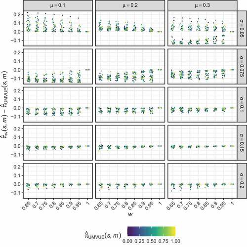
We begin with results for the case where $e=(\mathrm{\infty },6)$, $f=(1,5)$, and $n=(12,23)$. Figure 1 presents the difference between the optimised estimates, ${\hat{\pi }}_w(s,m)$, and the UMVUE estimates, ${\hat{\pi }}_{\mathrm{U}\mathrm{M}\mathrm{V}\mathrm{U}\mathrm{E}}(s,m)$, for the considered combinations of $\mu$ and $\sigma$, when $w\in \{0.65,0.7,0.75,\dots ,1\}$. It colours points corresponding to particular $(s,m)$ by the value of ${\hat{\pi }}_{\mathrm{U}\mathrm{M}\mathrm{V}\mathrm{U}\mathrm{E}}(s,m)$. Through this, it is clear that the difference in the optimised estimates and that of the UMVUE does not clearly depend on the value of ${\hat{\pi }}_{\mathrm{U}\mathrm{M}\mathrm{V}\mathrm{U}\mathrm{E}}(s,m)$. The range of differences between the optimised and UMVUE estimates is seen to be highly dependent on $\mu$ and $\sigma$. For example, in the case of $\mu =0.3$ and $\sigma =0.05$, the differences are large, which has implications for the bias and RMSE of these estimators (see below). For sent the corresponding results to the differences are by comparison very small; typically the optimised estimates modify the UMVUE by less than $0.01$.

Figure 1. Two-stage design. The distribution of the differences between the optimised estimates, ${\hat{\pi }}_w(s,m)$, and the UMVUE estimates, ${\hat{\pi }}_{\mathrm{U}\mathrm{M}\mathrm{V}\mathrm{U}\mathrm{E}}(s,m)$, are shown for several combinations of $\mu$ and $\sigma$, as a function of $w$. Points corresponding to particular $(s,m)$ are coloured by the value of ${\hat{\pi }}_{\mathrm{U}\mathrm{M}\mathrm{V}\mathrm{U}\mathrm{E}}(s,m)$.

Figures 2–3 present the performance of the optimised estimators in terms of their bias and RMSE respectively. It is clear that careful choice of $\mu$ and $\sigma$ is required to determine an optimised estimator that has performance that may be considered preferable to the UMVUE. Particularly for $\sigma =0.05$, several of the estimators exhibit large bias for values of $\pi$ only a small distance from $\mu$. Whilst for $\sigma \in \{0.15,0.2\}$, the performance of the optimised estimators is very similar to the UMVUE, indicating they provide little benefit. The same is true when $\mu =0.1$; only for $\mu \in \{0.2,0.3\}$ is performance substantially different from the UMVUE observed.

Figure 2. Two-stage design. The bias of the optimal estimators, $Bias({\hat{\pi }}_w|\pi )$, is shown for several combinations of $\mu$, $\sigma$, and $w$, as a function of $\pi$

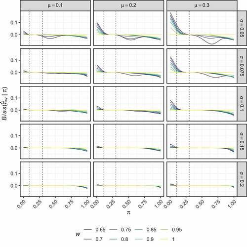
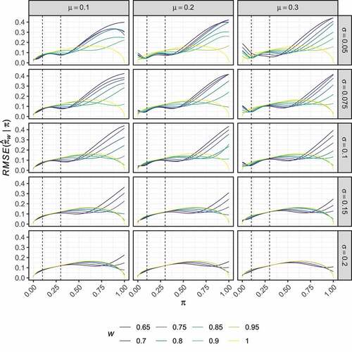
Figure 3. Two-stage design. The RMSE of the optimal estimators, $RMSE({\hat{\pi }}_w|\pi )$, is shown for several combinations of $\mu$, $\sigma$, and $w$, as a function of $\pi$.

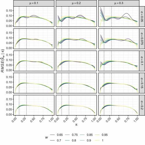
Particularly positive results are seen for $\sigma =0.1$ when $\mu =0.3$. We focus on the sub-case where $w=0.7$. The optimised estimator in this case maintains an absolute bias below $0.01$ when $\pi \in [0.119,0.806]$. For the cost of the larger bias introduced outside of this region, it has a lower RMSE than the UMVUE when $\pi \in [0.049,0.910]$. In particular, when $\pi =0.2$ and $\pi =0.3$, it reduces the RMSE compared to the UMVUE by 19.7% and 9.4% respectively. Table 1 presents the values of ${\hat{\pi }}_{\mathrm{U}\mathrm{M}\mathrm{V}\mathrm{U}\mathrm{E}}$ and ${\hat{\pi }}_{0.7}$ in this case. From this, it is clear that it achieves the efficiency gains whilst only making minor modifications to the UMVUE estimates for most values of $(s,m)$. Largest differences between ${\hat{\pi }}_{\mathrm{U}\mathrm{M}\mathrm{V}\mathrm{U}\mathrm{E}}(s,m)$ and ${\hat{\pi }}_{0.7}(s,m)$ are seen for smaller $s$; when the effect of the interim analysis on the final sample size is most pronounced. When the trial terminates in stage one (i.e., $s\le 1$) the optimised estimator adjusts the estimates upward compared to the UMVUE; effectively treating the interim termination as a ‘random low’. When the trial terminates in stage two with a low number of responses (i.e., $2\le s\le 6$) the optimised estimator adjusts the estimates downward in a pronounced manner compared to the UMVUE; effectively treating the continuation past the interim analysis as a ‘random high’.

Table 1. The UMVUE and example optimised estimates are given for the two-stage design with $e=\left(\mathrm{\infty },6\right)$, $f=\left(1,5\right)$, and $n=\left(12,23\right)$, and it’s non-stochastically curtailed extension. For the two-stage design, the optimised estimates correspond to $w=0.7$, $\mu =0.3$, and $\sigma =0.1$. For the non-stochastically curtailed design, the optimised estimates correspond to $w=0.8$, $\mu =0.3$, and $\sigma =0.1$. All values are given to 3 decimal places.

Two-stage design			Non-stochastically curtailed design
$(0,12)$	0.000	0.066	$(6,6)$	1.000	0.808
$(1,12)$	0.083	0.148	$(6,7)$	0.833	0.744
$(2,35)$	0.167	0.028	$(6,8)$	0.714	0.674
$(3,35)$	0.177	0.052	$(6,9)$	0.625	0.614
$(4,35)$	0.189	0.087	$(6,10)$	0.556	0.559
$(5,35)$	0.203	0.140	$(0,11)$	0.000	0.042
$(6,35)$	0.219	0.183	$(6,11)$	0.500	0.513
$(7,35)$	0.236	0.222	$(1,12)$	0.091	0.114
$(8,35)$	0.255	0.248	$(6,12)$	0.455	0.467
$(9,35)$	0.276	0.269	$(6,13)$	0.417	0.421
$(10,35)$	0.299	0.295	$(6,14)$	0.385	0.396
$(11,35)$	0.323	0.320	$(6,15)$	0.357	0.363
$(12,35)$	0.349	0.348	$(6,16)$	0.333	0.340
$(13,35)$	0.375	0.372	$(6,17)$	0.313	0.311
$(14,35)$	0.402	0.403	$(6,18)$	0.296	0.294
$(15,35)$	0.430	0.429	$(6,19)$	0.282	0.283
$(16,35)$	0.458	0.459	$(6,20)$	0.270	0.259
$(17,35)$	0.486	0.486	$(6,21)$	0.261	0.251
$(18,35)$	0.514	0.514	$(6,22)$	0.252	0.241
$(19,35)$	0.543	0.543	$(6,23)$	0.245	0.233
$(20,35)$	0.571	0.571	$(6,24)$	0.239	0.230
$(21,35)$	0.600	0.598	$(6,25)$	0.234	0.217
$(22,35)$	0.629	0.629	$(6,26)$	0.229	0.223
$(23,35)$	0.657	0.657	$(6,27)$	0.225	0.217
$(24,35)$	0.686	0.683	$(6,28)$	0.221	0.217
$(25,35)$	0.714	0.713	$(6,29)$	0.218	0.216
$(26,35)$	0.743	0.740	$(6,30)$	0.215	0.213
$(27,35)$	0.771	0.769	$(6,31)$	0.213	0.216
$(28,35)$	0.800	0.797	$(2,32)$	0.167	0.064
$(29,35)$	0.829	0.817	$(6,32)$	0.211	0.212
$(30,35)$	0.857	0.840	$(3,33)$	0.179	0.070
$(31,35)$	0.886	0.862	$(6,33)$	0.208	0.218
$(32,35)$	0.914	0.885	$(4,34)$	0.191	0.138
$(33,35)$	0.943	0.911	$(6,34)$	0.206	0.219
$(34,35)$	0.971	0.935	$(5,35)$	0.205	0.170
$(35,35)$	1.000	0.962	$(6,35)$	0.205	0.223

3.2. Non-stochastically curtailed design

Figures 4–6 present the corresponding results to Figures 1–3, but for the non-stochastically curtailed design. As before, Figure 4 displays no clear trend in the way the optimised estimators modify the UMVUE estimates. In this case, high bias is observed for larger values of $w$ than for the two-stage design setting (compare Figures 2 and 5). Here, the results for each considered $\mu$ are similar across the various values of $w$ and $\sigma$. However, $\mu =0.3$ typically results in slightly larger regions in which the bias remains small, and thus we now focus on this setting again.

Figure 4. Non-stochastically curtailed design. The distribution of the differences between the optimised estimates, ${\hat{\pi }}_w(s,m)$, and the UMVUE estimates, ${\hat{\pi }}_{\mathrm{U}\mathrm{M}\mathrm{V}\mathrm{U}\mathrm{E}}(s,m)$, are shown for several combinations of $\mu$ and $\sigma$, as a function of $w$. Points corresponding to particular $(s,m)$ are coloured by the value of ${\hat{\pi }}_{\mathrm{U}\mathrm{M}\mathrm{V}\mathrm{U}\mathrm{E}}(s,m)$.

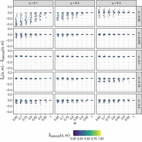
Figure 5. Non-stochastically curtailed design. The bias of the optimal estimators, $Bias({\hat{\pi }}_w|\pi )$, is shown for several combinations of $\mu$, $\sigma$, and $w$, as a function of $\pi$.

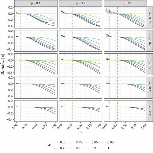
Figure 6. Non-stochastically curtailed design. The RMSE of the optimal estimators, $RMSE({\hat{\pi }}_w|\pi )$, is shown for several combinations of $\mu$, $\sigma$, and $w$, as a function of $\pi$.

Consider the optimal estimator for $\sigma =0.1$ and $w=0.8$. This estimator has an absolute bias of less than 0.01 for $\pi \in [0.079,0.527]$. It attains an RMSE lower than the UMVUE when $\pi \in [0.024,0.860]$; in particular when $\pi =0.2$ and $\pi =0.3$, it reduces the RMSE compared to the UMVUE by 8.6% and 2.4% respectively.

4. Discussion

Point estimation following a multi-stage single-arm trial is important to subsequent decision-making on a treatments development, to the inclusion of study results in to meta-analyses, and to the design of future trials. Whilst the UMVUE for such designs is well-established, it unfortunately can suffer from large RMSE compared to alternative estimators. However, these alternative estimators often have unsuitably large bias. Therefore, in this work we proposed methodology for finding estimators that are optimal for a particular objective function. Careful choice of the parameters that influence the value of the objective function was demonstrated for examples motivated by recent oncology trials (Collen et al. 2014; Jain et al. 2014; Lendvai et al. 2014; Schoffski et al. 2017; Shim et al. 2016) to result in an estimator that may be considered preferable to the UMVUE. The highlighted estimators retained low bias across a wide range of response rates, specifically those that should be more realistic based on the specified ${\pi }_0$ and ${\pi }_1$, and reduced the RMSE for certain response rates by a large amount compared to the UMVUE. Especially strong performance was seen in the two-stage setting, where the RMSE of the optimal estimator with $\mu =0.3$, $\sigma =0.1$, and $w=0.7$ reduced the RMSE by as much as 35.2% ($\pi =0.107$).

We note some limitations to our work. Firstly, we consider only three possible sets of design parameters $e$, $f$, and $n$. Whilst there is no reason to assume optimised estimators that can rival the UMVUE in terms of their properties cannot be determined for other possible parameter combinations, there is also no reason to assume that they can. In addition, we focused on an objective function composed of the the marginal absolute bias and RMSE. Conditional bias and RMSE may also be of concern in general (Fan et al. 2004; Liu et al. 2004; Shimura et al. 2018; Troendle and Yu 1999). Our objective function, of course, could be readily modified to take conditional bias and RMSE in to consideration if desired, though. Furthermore, in the Supplementary Materials, we also consider the use of squared-bias and MSE. Finally, our determinations assume that the planned design will be realised in practice. Of course, this may not always be the case, and while effective procedures are now available to control the type-I error-rate in this case (Englert and Kieser 2015), our work does not assist in determining the best estimator when the design is likely to under/over-run.

Arguably the biggest barrier to the use of our approach in practice is how to specify the values of $\mu$, $\sigma$, and $w$, such that the estimator is well justified. As noted, a possible solution is to elicit values of $\mu$ and $\sigma$ based on available expertise on the anticipated response rate of the treatment under investigation (or the parameters of an appropriate Beta distribution; see the Supplementary Materials). A potentially preferential approach is to simply treat $\mu$, $\sigma$, and $w$ as nuisance parameters. By specifying, e.g., a range of values for $\pi$ over which it is desired for the absolute bias to be constrained to some maximal amount, and similarly particular target reductions in the RMSE over the UMVUE for given values of $\pi$, one could simply perform a further optimisation over $\mu$, $\sigma$, and $w$ to determine the estimator with the best performance.

Given our work is motivated by a desire to see the increased utilisation of adjusted estimators, we end with a brief discourse on communicating why this is an important problem and how it may be handled to non-statistical stakeholders. Fundamentally, as discussed, the inclusion of an interim analysis will bias the results of trial inference if appropriate adjustments are not made. The estimated treatment effect is not only critical to deciding the development plan for the current treatment under investigation, but also potentially to other treatments investigated downstream. Thus, some adjustment should be made. Unfortunately, Grayling and Mander (2021) recently demonstrated that very few phase II oncology trials currently make such adjustments, meaning many reported effects may be subject to appreciable bias. On specifically how to adjust, we would argue it is not important for non-statistical stakeholders to understand exactly how adjusted estimators ‘work’. They can, and arguably should, however, feed in to the decision on which adjusted estimator to use; simple explanations of bias and RMSE can let them help guide that factor is of larger concern. Then, whatever method is used, a table like that given here (Table 1) can always be produced for any trial before its completion. Thus, even for more complex estimators the actual estimation remains as simple as reading from a pre-prepared table.

In conclusion, the proposed methodology for determining optimised estimators may allow the determination of an estimator that has low bias for many possible, arguably more likely, values of the response rates whilst providing reduced RMSE compared to the UMVUE across these response rates. For certain values of the response rate, this reduction in the RMSE may be sizeable.

Data availability statement

Code to reproduce all results given in this manuscript is available from https://github.com/mjg211/article_code.

Disclosure statement

No potential conflict of interest was reported by the author(s).

Supplementary material

Supplemental data for this article can be accessed on the publisher’s website

Additional information

Funding

This research did not receive any specific grant from funding agencies in the public, commercial, or not-for-profit sectors.

References

- Armitage, P. 1957. Restricted sequential procedures. Biometrika 44:9–56. doi:10.1093/biomet/44.1-2.9.
- Chang, M., H. Wieand, and V. Chang. 1989. The bias of the sample proportion following a group sequential phase II clinical trial. Statistics in Medicine 8:563–570. doi:10.1002/sim.4780080505.
- Chen, T. 1997. Optimal three-stage designs for phase II cancer clinical trials. Statistics in Medicine 16:2701–2711. doi:10.1002/(SICI)1097-0258(19971215)16:23<2701::AID-SIM704>3.0.CO;2-1.
- Collen, C., N. Christian, D. Schallier, M. Meysman, M. Duchateau, G. Storme, and M. De Ridder. 2014. Phase II study of stereotactic body radiotherapy to primary tumor and metastatic locations in oligometastatic nonsmall-cell lung cancer patients. Annals of Oncology 25:1954–1959. doi:10.1093/annonc/mdu370.
- Eisenhauer, E., P. Therasse, J. Bogaerts, L. Schwartz, D. Sargent, R. Ford, J. Dancey, S. Arbuck, S. Gwyther, and M. Mooney, et al. 2009. New response evaluation criteria in solid tumours: Revised RECIST guideline (version 1.1). European Journal of Cancer 45:228–247. doi:10.1016/j.ejca.2008.10.026.
- Englert, S., and M. Kieser. 2015. Methods for proper handling of overrunning and underrunning in phase II designs for oncology trials. Statistics in Medicine 34:2128–2137. doi:10.1002/sim.6479.
- Fairbanks, K., and R. Madsen. 1982. P values for tests using a repeated significance test design. Biometrika 69:69–74.
- Fan, X., D. DeMets, and K. Lan. 2004. Conditional bias of point estimates following a group sequential test. Journal of Biopharmaceutical Statistics 14:505–530. doi:10.1081/BIP-120037195.
- Girshick, M., F. Mosteller, and L. Savage. 1946. Unbiased estimates for certain binomial sampling problems with applications. The Annals of Mathematical Statistics 17:13–23. doi:10.1214/aoms/1177731018.
- Grayling, M., M. Dimairo, A. Mander, and T. Jaki. 2019. A review of perspectives on the use of randomization in phase II oncology trials. Journal of the National Cancer Institute 111:1255–1262. doi:10.1093/jnci/djz126.
- Grayling, M., and A. Mander. 2021. Two-stage single-arm trials are rarely analyzed effectively or reported adequately JCO Precision Oncology 5 1813–1820. doi:10.1200/PO.21.00276 .
- Guo, H., and A. Liu. 2005. A simple and efficient bias-reduced estimator of response probability following a group sequential phase II trial. Journal of Biopharmaceutical Statistics 15:773–781. doi:10.1081/BIP-200067771.
- Jain, N., E. Curran, N. Iyengar, E. Diaz-Flores, R. Kunnavakkam, L. Popplewell, M. Kirschbaum, T. Karrison, H. Erba, and M. Green, et al. 2014. Phase II study of the oral MEK inhibitor selumetinib in advanced acute myelogenous leukemia: A University of Chicago phase II consortium trial. Clinical Cancer Research 20:490–498. doi:10.1158/1078-0432.CCR-13-1311.
- Jennison, C., and B. Turnbull. 1983. Confidence intervals for a binomial parameter following a multistage test with application to MIL-STD 105D and medical trials. Technometrics 25:49–58. doi:10.1080/00401706.1983.10487819.
- Jung, S., and K. Kim. 2004. On the estimation of the binomial probability in multistage clinical trials. Statistics in Medicine 23 (6):881–896. doi:10.1002/sim.1653.
- Jung, S., T. Lee, K. Kim, and S. George. 2004. Admissible two-stage designs for phase II cancer clinical trials. Statistics in Medicine 23 (4):561–569. doi:10.1002/sim.1600.
- Koyama, T., and H. Chen. 2008. Proper inference from Simon’s two-stage designs. Statistics in Medicine 27 (16):3145–3154. doi:10.1002/sim.3123.
- Kunzmann, K., and M. Kieser. 2018. Test-compatible confidence intervals for adaptive two-stage single-arm designs with binary endpoint. Biometrical Journal 60 (1):196–206. doi:10.1002/bimj.201700018.
- Law, M., M. Grayling, and A. Mander. 2022. A stochastically curtailed single‐arm phase II trial design for binary outcomes Journal of Biopharmaceutical Statistics doi:10.1080/10543406.2021.2009498 . .
- Lendvai, N., P. Hilden, S. Devlin, H. Landau, H. Hassoun, A. Lesokhin, I. Tsakos, K. Redling, G. Koehne, D. Chung, et al. 2014. A phase 2 single-center study of carfilzomib 56 mg/m2 with or without low-dose dexamethasone in relapsed multiple myeloma. Blood 124 (6):899–906. doi:10.1182/blood-2014-02-556308.
- Li, Q. 2011. An MSE-reduced estimator for the response proportion in a two-stage clinical trial. Pharmaceutical Statistics 10 (3):277–279. doi:10.1002/pst.414.
- Liu, A., J. Troendle, K. Yu, and V. Yuan. 2004. Conditional maximum likelihood estimation following a group sequential test. Biometrical Journal 46 (6):760–768. doi:10.1002/bimj.200410076.
- Mander, A., and S. Thompson. 2010. Two-stage designs optimal under the alternative hypothesis for phase II cancer clinical trials. Contemporary Clinical Trials 31 (6):572–578. doi:10.1016/j.cct.2010.07.008.
- Mander, A., J. Wason, M. Sweeting, and S. Thompson. 2012. Admissible two-stage designs for phase II cancer clinical trials that incorporate the expected sample size under the alternative hypothesis. Pharmaceutical Statistics 11 (2):91–96. doi:10.1002/pst.501.
- Pepe, M., Z. Feng, G. Longton, and J. Koopmeiners. 2009. Conditional estimation of sensitivity and specificity from a phase 2 biomarker study allowing early termination for futility. Statistics in Medicine 28 (5):762–779. doi:10.1002/sim.3506.
- Porcher, R., and K. Desseaux. 2012. What inference for two-stage phase II trials? BMC Medical Research Methodology 12:117 doi:10.1186/1471-2288-12-117.
- Schoffski, P., A. Wozniak, S. Stacchiotti, P. Rutkowski, J. Blay, L. Lindner, S. Strauss, A. Anthoney, F. Duffaud, and S. Richter, et al. 2017. Activity and safety of crizotinib in patients with advanced clear-cell sarcoma with met alterations: European organization for research and treatment of cancer phase II trial 90101 ‘CREATE’. Annals of Oncology 28 (12):3000–3008. doi:10.1093/annonc/mdx527.
- Schultz, J., F. Nichol, G. Elfring, and S. Weed. 1973. Multiple-stage procedures for drug screening. Biometrics 29 (2):293–300. doi:10.2307/2529393.
- Scrucca, L. 2017. On some extensions to GA package: Hybrid optimisation, parallelisation and islands evolution. The R Journal 9 (1):187–206. doi:10.32614/RJ-2017-008.
- Shim, H., K. Kim, J. Hwang, W. Bae, S. Ryu, Y. Park, T. Nam, I. Chung, and S. Cho. 2016. A phase II study of adjuvant S-1/cisplatin chemotherapy followed by S-1-based chemoradiotherapy for D2-resected gastric cancer. Cancer Chemotherapy and Pharmacology 77 (3):605–612. doi:10.1007/s00280-016-2973-2.
- Shimura, M., K. Maruo, and M. Gosho. 2018. Conditional estimation using prior information in 2-stage group sequential designs assuming asymptotic normality when the trial terminated early. Pharmaceutical Statistics 17 (5):400–413. doi:10.1002/pst.1859.
- Siegmund, D. 1978. Estimation following sequential tests. Biometrika 65 (2):341–349. doi:10.2307/2335213.
- Simon, R. 1989. Optimal two-stage designs for phase II clinical trials. Controlled Clinical Trials 10 (1):1–10. doi:10.1016/0197-2456(89)90015-9.
- Troendle, J., and K. Yu. 1999. Conditional estimation following a group sequential clinical trial. Communications in Statistics - Theory and Methods 28 (7):1617–1634. doi:10.1080/03610929908832376.
- Tsai, W., Y. Chi, and C. Chen. 2008. Interval estimation of binomial proportion in clinical trials with a two-stage design. Statistics in Medicine 27 (1):15–35. doi:10.1002/sim.2930.
- Tsiatis, A., G. Rosner, and C. Mehta. 1984. Exact confidence intervals following a group sequential test. Biometrics 40 (3):797–803. doi:10.2307/2530924.