Non-inferiority testing for qualitative microbiological methods:Assessing and improving the approach in USP <1223>

ABSTRACT

The United States Pharmacopoeia (USP) presents two approaches for showing non-inferiority of an alternate qualitative microbiological method versus a compendial method. One approach compares the positive rates for the alternate and compendial methods at one spike level, while the other one compares multiple most probable number (MPN) estimates from a multi-spike design using a t-test. In this paper, we discuss these approaches under certain assumptions and propose a third approach that can be used for both single and multiple dilutions, which we call the generalized MPN (gMPN) approach. Simulations, using Poisson distributed numbers of microorganisms in test samples, confirm that the USP approach based on rates is not suitable, that the USP approach based on MPNs is appropriate for non-inferiority, but the gMPN approach outperforms the MPN-based approach and is therefore recommended.

KEYWORDS:

• Binomial detection
• detection proportion
• limit of detection
• microbiological validation
• most probable number
• sterility tests

1. Introduction

To show that a new or alternative qualitative microbiological method is acceptable to replace a current or compendial method, the USP <1223> (2015) guideline states that the laboratory must demonstrate that the new procedure is as good as or better than the current procedure in terms of the ability to detect microorganisms. The USP recommends non-inferiority testing, for which it proposes two different approaches.

The first approach is based on the ratio of the proportions $p_A$ and $p_C$ of positive samples for the alternative and the compendial method at a single spike level, respectively, similar to non-inferiority of clinical events in clinical trials. A pre-defined non-inferiority margin quantifies what difference is allowed. The second approach is based on a comparison of the most probable numbers (MPN) using a design with multiple dilutions (Cochran 1950). Absence/presence results obtained from multiple dilutions are used to estimate one bacterial density of organisms in the original solution. This is done multiple times with the alternative and the compendial method to create repeated estimates of the bacterial density. Then non-inferiority is tested on two sets of MPNs using a t-test.

The USP does not provide guidance when to use which of the two non-inferiority approaches, neither discusses how to interpret the results from these approaches. Based on a statistical model for the detection of microorganisms (IJzerman-Boon and Van den Heuvel 2015), we will assess and improve the non-inferiority approaches.

Section 2 describes the two USP approaches, on positive rates and on MPNs, as well as their implicit assumptions. Section 3 describes the statistical detection model and proposes a third approach (the generalized MPN approach). Section 4 presents different experimental designs to determine MPN estimates and explains that under the described distributional assumptions, results for testing non-inferiority with the MPN are not expected to differ. Subsequently, Sections 5 and 6 describe our simulation study and present the results, respectively. Section 7 presents (a discussion on) our conclusions.

2. Non-inferiority testing according to USP <1223>

2.1. Approach 1: non-inferiority on positive rates

In order to show non-inferiority, it is required that both methods test similar sets of samples (see Section 2.3 for details). The null hypothesis is then formulated as $H_0:p_A/p_C\le r_0$ against the alternative hypothesis $H_1:p_A/p_C>r_0$, with $r_0\in \left(0,1\right)$ the non-inferiority margin. By proposing a non-inferiority margin of −0.2 for the difference $p_A-p_C$, the USP indirectly suggests a non-inferiority margin of $r_0=0.8$ for the ratio. Following Farrington and Manning (1990), the null hypothesis can be rewritten as $H_0:p_A-r_0{p}_C\le 0$, and is rejected when

(1) $\left({\hat{p}}_A-r_0{\hat{p}}_C\right)/{\hat{w}}_0^{1/2}>z_{1-\alpha },$(1)

with $z_{1-\alpha }$ the $100\left(1-\alpha \right)\mathrm{\%}$ percentile of the standard normal distribution, ${\hat{p}}_A$ and ${\hat{p}}_C$ the standard estimates of the probabilities $p_A$ and $p_C$ to detect positive test samples, and ${\hat{w}}_0$ the estimated variance of ${\hat{p}}_A-r_0{\hat{p}}_C$ under the null hypothesis. Thus, when $X_A$ and $X_C$ are the numbers of positive samples among $n_A$ and $n_C$ test samples tested with the alternative and compendial method, respectively, we have ${\hat{p}}_A=X_A/n_A$, ${\hat{p}}_C=X_C/n_C$, and ${\hat{w}}_0$ is

(2) ${\hat{w}}_0={\tilde{p}}_A\left(1-{\tilde{p}}_A\right)/n_A+r_0^2{\tilde{p}}_C\left(1-{\tilde{p}}_C\right)/n_C,$(2)

with ${\tilde{p}}_A$ and ${\tilde{p}}_C$ the maximum likelihood estimators (MLE) under the null hypothesis, i.e. ${\tilde{p}}_C={\tilde{p}}_A/r_0$, ${\tilde{p}}_A=\left[-b-{\left(b^2-4ac\right)}^{1/2}\right]/\left(2a\right)$, $a=1+k$, $b=-\left[r_0\left(1+k{\hat{p}}_C\right)+k+{\hat{p}}_A\right]$, $c=r_0\left({\hat{p}}_A+k{\hat{p}}_C\right)$, and $k=n_C/n_A$. A 5% significance level is used, i.e. $\alpha =0.05$.

Note that this approach is applicable to test samples from a single dilution, since a clear extension to multiple dilutions (with different probabilities for testing positives) is not known. The USP recommends a spike level of microorganisms for this dilution at which 50–75% of the samples would be expected to be positive when tested with the compendial method.

If, instead of testing independent samples from a single dilution with the alternative and compendial method, the same $n$ samples are tested by both methods, then the results can be displayed in a 2 × 2 table (Table 1), and a paired test can be applied. In formula (1), we then use (Lachenbruch and Lynch 1998) ${\hat{p}}_A=X_A/n=\left(X_{11}+X_{10}\right)/n$, ${\hat{p}}_C=X_C/n=\left(X_{11}+X_{01}\right)/n$, resulting in ${\hat{p}}_A-r_0{\hat{p}}_C=\left(X_{10}+\left(1-r_0\right)X_{11}-r_0{X}_{01}\right)/n$, and we replace the variance estimate (2) by

Table 1. Lay-out of results for a paired test – Numbers of positive and negative samples (associated probabilities).

	Compendial method
Alternative method	Positive	Negative	Row total
Positive	$X_{11}$ ($p_{11})$	$X_{10}$ ($p_{10})$	$X_A$ ($p_A)$
Negative	$X_{01}$ ($p_{01})$	$X_{00}$ ($p_{00})$	$n-X_A$ ($1-p_A)$
Column total	$X_C$ ($p_C)$	$n-X_C$ ($1-p_C)$	n ($1)$

(3) $\begin{array}{rl}{\hat{w}}_0=& [{\hat{p}}_{10}\left(1-{\hat{p}}_{10}\right)+{\left(1-r_0\right)}^2{\hat{p}}_{11}\left(1-{\hat{p}}_{11}\right)+r_0^2{\hat{p}}_{01}\left(1-{\hat{p}}_{01}\right)\\ & +2r_0{\hat{p}}_{10}{\hat{p}}_{01}-2\left(1-r_0\right){\hat{p}}_{10}{\hat{p}}_{11}+2r_0\left(1-r_0\right){\hat{p}}_{01}{\hat{p}}_{11}]/n,\end{array}$(3)

where ${\hat{p}}_{ij}=X_{ij}/n$. Note that USP <1223> incorrectly suggests a variance of $X_A\left(X_{10}+X_{01}\right)/X_C^3$, which is an estimate of the variance of ${\hat{p}}_A/{\hat{p}}_C$ instead of ${\hat{p}}_A-r_0{\hat{p}}_C$.

2.2. Approach 2: non-inferiority on MPNs

For the MPN-based approach, the null hypothesis $H_0:log\left(\lambda { }_A\right)-\mathrm{l}\mathrm{o}\mathrm{g}\left(\lambda { }_C\right)\le \mathrm{l}\mathrm{o}\mathrm{g}\left(r_0\right)$ needs to be rejected in favor of $H_1:log\left(\lambda { }_A\right)-log\left(\lambda { }_C\right)>\mathrm{l}\mathrm{o}\mathrm{g}\left(r_0\right)$, where $\lambda {}_A$ and $\lambda {}_C$ are the theoretical bacterial densities for the alternative and compendial method, respectively. Following Cochran (1950), the probability that a sample is tested positively equals $p=1-exp(-\lambda )$, when λ is the mean number of organisms in the test samples and the microbiological method detects organisms perfectly. Given an estimate $\hat{p}\in \left(0,1\right)$ for the proportion $p$, based on test samples with volume $v$ taken from a single solution with volume $V$, the bacterial density and corresponding number of organisms in the solution are estimated by

(4) $\hat{\lambda }=-\mathrm{l}\mathrm{o}\mathrm{g}\left(1-\hat{p}\right)\mathrm{a}\mathrm{n}\mathrm{d}\widehat{MPN}=\left(V/v\right)\hat{\lambda }.$(4)

The MPN can also be estimated from a multiple dilution experiment, but then a closed-form expression does not exist.

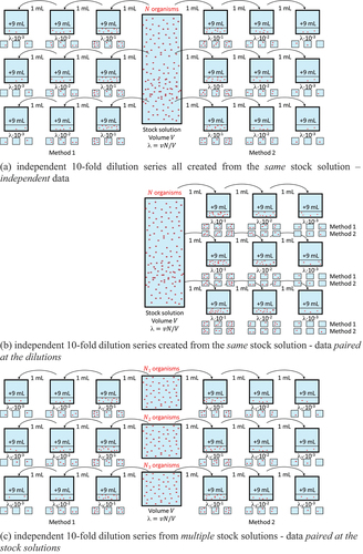
Based on $N_A$ and $N_C$ MPN estimates or replicates for the two methods, respectively, a t-test for non-inferiority can be applied to the log-transformed estimates. Note that there are different ways of generating these MPN estimates (further discussed in Section 4), but when all MPNs are trying to estimate the same bacterial density and are estimated based on independent samples from the same stock solution (Figure 2a), then a two-sample t-test can be used. If ${\bar{Y}}_A$ and $S_A$ denote the average and standard deviation of the $N_A$ estimates for $log\left(\lambda { }_A\right)$ (or equivalently, for $log\left(MP{N}_A\right)$) for the alternative method, and ${\bar{Y}}_C$, $S_C$, and $N_C$ for the compendial method, then non-inferiority can be concluded if

Figure 1. Visualization of conditional and marginal probabilities (7) and (8)

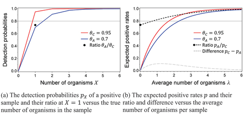
Figure 2. Experiments to generate multiple MPN estimates in a 3 × 3 design for 2 methods.

(5) ${\bar{Y}}_A-{\bar{Y}}_C-t_{1-\alpha ,df}\sqrt{\frac{S_A^2}{N_A}+\frac{S_C^2}{N_C}}>\mathrm{l}\mathrm{o}\mathrm{g}\left(r_0\right),$(5)

where $t_{1-\alpha ,\hspace{0.17em}df}$ denotes the $100\left(1-\alpha \right)\mathrm{\%}$ percentile of the t-distribution with the Satterthwaite degrees of freedom

$df=\frac{{\left(S_A^2/N_A+S_C^2/N_C\right)}^2}{\frac{{\left(S_A^2/N_A\right)}^2}{N_A-1}+\frac{{\left(S_C^2/N_C\right)}^2}{N_C-1}}.$

In case the MPNs for the two methods are estimated based on samples from the same dilutions (Figure 2b), even though in this case the two methods do not test the exact same samples, a paired t-test may be more appropriate. When $\bar{Y}$ and $S^2$ denote the sample mean and sample variance of the $N$ paired differences $\hat{Y}=log\left({\hat{\lambda }\hspace{0.17em}}_A\right)-log\left({\hat{\lambda }\hspace{0.17em}}_C\right)$ of the log-transformed MPN estimates for the alternative method minus the compendial method, then non-inferiority can be concluded if

(6) $\bar{Y}-t_{1-\alpha ,N-1}\frac{S}{\sqrt{N}}>\mathrm{l}\mathrm{o}\mathrm{g}\left(r_0\right).$(6)

2.3. Implicit assumptions in USP

In the first approach, the non-inferiority claim would only hold for the tested spike that resulted in the positive rates for which non-inferiority could be concluded. At that spike level, and under the assumption that both methods indeed received samples with similar spike levels, the two methods are likely to come to the same pass or fail conclusion. In the USP, this is referred to as decision equivalence. However, decision equivalence does not at all imply that the two microbiological methods have approximately the same sensitivity. To illustrate this, think of two microbiological methods, one detecting only molds, and one detecting only bacteria. When samples with mixtures of bacteria and molds are offered to both methods, the positive rates may be equivalent for the two methods. Nevertheless, it is obvious that the methods do not have the same sensitivity for both types of microorganisms and as a microbiologist you would never rely on just one method. Another situation where two methods might appear to be similar, is if you offer samples with a high spike. Then, even a poor test method will return only positive results. In these examples, it is clear that the number of positive samples does not only depend on the microbiological method, but also on the numbers of organisms in the test samples, and non-inferiority for one spike level (e.g. the level at which 50–75% of the samples would be positive with the compendial method) does not necessarily imply non-inferiority at other spike levels.

Another implicit assumption is that all samples have the same fixed probability ($p_A$ or $p_C$ depending on the test method), of becoming positive. This would be reasonable only when all samples contain the same number of organisms, but creating samples with a fixed number of organisms is currently impossible in microbiology. Even when all samples are taken from the same solution, numbers of organisms will vary from sample to sample because of sampling variability, and therefore some samples have lower probabilities of being detected positively than other samples.

In the second approach, the MPN method implicitly assumes that organisms are distributed randomly and unaggregated throughout the solution, such that the number of organisms in a small amount or test sample taken from it follows a Poisson distribution (Cochran 1950; Garthright and Blodgett 1996). Samples are assumed independent of each other (Garthright and Blodgett 1996), which means that the probability of a sample to be positive is not affected by other samples being positive or negative. This is practically true when the total volume of all samples constitutes a small volume of the total solution, say less than 10%.

Additionally, as Cochran (1950) phrased it for growth-based methods: “each sample, when incubated in the culture medium, is certain to exhibit growth when it contains one or more microorganisms”. This would imply that every organism is detected by the method. But, if perfect detection is already part of our assumptions, what are we demonstrating when we show non-inferiority on MPNs?

3. Non-inferiority testing based on a statistical model for the detection of microorganisms

Since the number of positive test samples is not only determined by the method, but also by the unknown spike, we need an appropriate model that describes how a positive result is achieved and that can separate the spike level from the sensitivity of the method. To do this, we introduce two concepts the first concept describes the detection probability to detect one sample as positive as a function of the true number of organisms in the sample, the second concept considers a distribution for this unknown true number of organisms when we sample from a solution. Full knowledge of the first concept of the model would provide full insight into the sensitivity of the method for each possible number of organisms in the test sample. The detection probability, which should be an increasing function of the number of microorganisms $X$ in the sample, may have parameters that would characterize the performance of the method.

3.1. The binomial-Poisson model

Denote the outcome of the test sample by $Z$, which would be 0 for a negative result, and 1 for a positive result. A simple model (IJzerman-Boon and Van den Heuvel 2015; Van den Heuvel and IJzerman-Boon 2013) assumes that each microorganism has a fixed probability $\theta$ (between 0 and 1) to be detected by the microbiological test method. This parameter has been called the detection proportion and represents the probability to detect one organism. The detection probability $p_X$ that the microbiological test would return a positive test result for a sample, i.e. detect at least one organism, can be expressed as a conditional probability given the number of organisms $X$ in the sample,

(7) $p_X=P(Z=1|X)=1-{\left(1-\theta \right)}^X.$(7)

This model has been referred to as the binomial detection model, since it is based on the binomial distribution when the method detects organisms independently from each other. Note that for $X=1$, the detection probability $p_1$ reduces to the detection proportion $\theta$.

Unfortunately, it is impossible to spike test samples with a fixed number of microorganisms. The spike exhibits variability, and therefore we cannot observe the function (7) directly. If the spikes $X$ follow a Poisson distribution with a mean of $\lambda$, which is a common and often a reasonable distributional model for count data (Cochran 1950), then the marginal probability to detect a sample as positive equals the expected positive rate $p$ and can be written as

(8) $p=P\left(Z=1\right)=1-exp\hspace{0.17em}\left(-\theta \lambda \right).$(8)

A graphical representation of (7) and (8) is provided in Figure 1.

Based on an experiment, we can estimate the expected positive rate $p$ from (8) as described earlier. However, the sensitivity of the method is reflected by the parameter $\theta$, which cannot be separated from the average spike per test sample $\lambda$. We can only estimate the product $\xi =\theta \lambda$. For a single dilution, it is estimated by

(9) $\hat{\xi }=-\mathrm{l}\mathrm{o}\mathrm{g}\left(1-\hat{p}\right),$(9)

and its corresponding variance would be estimated by ${\hat{\tau }}^2=\hat{p}/\left(n\left(1-\hat{p}\right)\right)$ (IJzerman-Boon and Van den Heuvel 2015). Note that for $\theta =1$, this estimator is just the MPN estimator for the bacterial density $\lambda$ (Cochran 1950), presented in (4). Hence, our binomial detection model with $\theta <1$ can be viewed as a generalization of the MPN and will be referred to as the generalized MPN.

3.2. Approach 3: non-inferiority on generalized MPNs

Observing that what we estimate is generally not the bacterial density itself, but its product with the detection proportion, it becomes clear that comparing the two test methods should be done by considering the ratio ${\xi }_A/{\xi }_C$, which equals the accuracy or recovery ${\theta }_A/{\theta }_C$, provided both methods tested samples from the same solution with an average spike of $\lambda$ per test sample. Taking the ratio eliminates the spike level $\lambda$ from the test statistic. Testing from the same solution is important, since otherwise the average spike $\lambda$ does not cancel out when taking the ratio. This recovery or accuracy quantifies the relative performance of two qualitative methods and can be used to test non-inferiority of the alternative method compared to the compendial method (EP 5.1.6 2017).

Approximate confidence limits for this ratio ${\theta }_A/{\theta }_C$ or its logarithm $log\left({\theta }_A/{\theta }_C\right)$ have been derived in IJzerman-Boon and Van den Heuvel (2015). Since in the log-scale a coverage is obtained that is closer to the nominal level, non-inferiority would be concluded if

(10) $\mathrm{l}\mathrm{o}\mathrm{g}\left({\hat{\xi }}_A/{\hat{\xi }}_C\right)-z_{1-\alpha }\sqrt{{\hat{\tau }}_C^2/{\hat{\xi }}_C^2+{\hat{\tau }}_A^2/{\hat{\xi }}_A^2}>\mathrm{l}\mathrm{o}\mathrm{g}\left(r_0\right),$(10)

where $z_{1-\alpha }$ is the $100\left(1-\alpha \right)\mathrm{\%}$ percentile of the standard normal distribution.

Expressions (9) and (10) hold for a single dilution. Like with the MPN method, also multiple dilution experiments can be used to estimate the (ratio of) detection proportions and corresponding confidence limits using maximum likelihood, but closed-form expressions do not exist anymore (IJzerman-Boon and Van den Heuvel 2015). Then, a statistical package like SAS® can be used to perform the calculations.

3.3. Comparing the gMPN with the USP non-inferiority methods

Figure 1 (solid lines) displays functions (7) and (8) for different values of the detection proportion $\theta$, where ${\theta }_C=0.95$ might reflect the compendial method and ${\theta }_A=0.7$ the alternative method. Figure 1a shows the detection probabilities that we are interested in, since it provides the performance of the alternative and compendial method when they would test samples with a fixed number of microorganisms. When using a non-inferiority margin of $r_0=$ 0.8 in this example, the alternative method is obviously inferior compared to the compendial method, since the ratio ${\theta }_A/{\theta }_C$ (black dot) of the two detection proportions for detecting samples with exactly one microorganism ($X=1$) is smaller than the non-inferiority margin $r_0$ (reference line). Note that it is irrelevant that the ratio of the detection probabilities for samples with higher numbers of microorganisms ($X>1$) is larger than 0.8, since the methods are inferior for detecting one microorganism and thus inferior in detecting microorganisms. Figure 1b reflects the expected positive rates ($p_C$ for the compendial and $p_A$ for the alternative method) that we would observe in experimental data as a function of the average spike level. Since test samples will vary in their number of microorganisms in practice, they average out the detection probabilities in Figure 1a into the positive rates. Figure 1b also shows the ratio (dark dashed line) of these expected positive rates that is used to test non-inferiority in the first USP approach and the difference in positive rates (light dashed line). For $\lambda =0$, the ratio starts at ${\theta }_A/{\theta }_C$ and then increases to 1 for higher spike levels. Thus, theoretically we would be able to demonstrate inferiority of the alternative method with respect to the compendial method using the ratio of positive rates when we would be able to create a dilution with an average number of microorganisms below, say, 0.7, since then the ratio of positive rates is less than 0.8 as well. However, there are a few practical concerns. First of all, spiking dilutions is (very) imprecise, and we may easily end up with an average spike (far) above 0.7, in which case we may declare the alternative method non-inferior (since the ratio of positive rates is then above the non-inferiority margin of 0.8). Secondly, the USP suggests spike levels for experimentation for which the positive rate of the compendial method is between 50% and 75%, i.e., spike levels that would result in non-inferiority since they provide ratios of the positive rates above the non-inferiority margin. Performing the experiment in this range would suggest the use of a difference in positive rates, since it does provide the largest absolute difference between the two methods, but the difference in positive rates ($p_C-p_A$) would never be larger than 0.2 (an equivalent non-inferiority margin for differences when the ratio is 0.8 and the compendial method is close to perfect) for any of the spike levels (see the difference curve at the bottom of Figure 1b). Thirdly, even if we would be able to create low spike levels, the ratio of the positive rates still provides a somewhat better result than the ratio of detection proportions ${\theta }_A/{\theta }_C$ since it is larger than this ratio, unless we would spike very close to the level of blank samples, but then this would blow up the standard error of the estimated ratio and it would require very large numbers of samples. Finally, even if one would be willing to be less stringent and, instead of requiring non-inferiority on detecting a single organism, only require non-inferiority on the positive rates from a certain spike level onwards (probably at a more stringent non-inferiority margin), the uncertainty of the spike remains a problem, since it is impossible to estimate at which spike level the non-inferiority conclusion was drawn, nor does it tell anything about detection at lower spike levels or of just one organism.

Comparing formula (10) on generalized MPNs with formulas (5) and (6) on MPNs shows that both approaches actually evaluate the same thing, since the logarithm of a ratio equals the difference of the logarithms. Although the MPN approach implicitly assumes that the method is perfect, the similarity between (4) and (9) explains why a difference between MPNs, which would be an internal conflict with the assumption that two perfect methods are used to estimate the bacterial density of the same solution, may be attributed to or interpreted as a difference in detection between the two methods. The difference between the MPN approach and the generalized MPN approach is that in the latter approach all data are used to come up with one combined generalized MPN estimate for the ratio ${\xi }_A/{\xi }_C$ and its standard error, while in the MPN approach, first multiple MPN estimates are generated and those are used as the data in the calculations.

4. Independent and paired experimental designs for the MPN approach

MPN experiments with multiple dilutions can be executed in different ways. One way is to generate all MPN estimates for both methods based on independent dilution series from the same stock solution (Figure 2a). This implies that the MPNs can be considered independent estimates for the same bacterial density and that the two-sample t-test for independent samples can be used. Instead of creating different dilution series per method, one could take samples for both methods from the same dilutions simultaneously (Figure 2b). This would prevent that potential pipetting errors in creating the dilutions would lead to different results between the methods. This experiment provides paired data at the level of the dilutions. There is no formal approach mentioned in the USP to properly address this pairing, but the paired MPN t-test, in the USP only suggested for the rare case where the exact same samples are tested with both methods, is applicable to this design as well.

An alternative for both cases, which may be more practical if testing cannot be performed on one day, would be that multiple stock solutions are used, from each of which one dilution series is created for the alternative method and one for the compendial method (Figure 2c). In this case, data are paired at the level of the stock solutions. The disadvantage of this paired design is that the bacterial densities will vary with stock solution due to variation in spiking. Nevertheless, the paired MPN t-test can be applied in this case.

Finally, one could use different stock solutions for the two methods, but this should be avoided, because differences observed between the two methods might then be caused by differences in the spikes $\lambda$ for the two methods, rather than differences in detection by the methods.

In general, these different designs and ways of pairing samples may lead to different correlation structures between the samples. This might require different statistical analysis methods or, when analyzed using the same statistical methods ignoring correlations, could lead to different results. If, however, the number of organisms $N$ in the stock solution follows a Poisson distribution and samples are generated from that solution using binomial or multinomial sampling, then the numbers of organisms in the individual samples also follow a Poisson distribution. In addition, independence between the samples can be proven in this case, even though the experimental design suggests dependent samples (Appendix 1). Under this assumption, it therefore does not matter whether the different samples are collected in an independent or dependent way. This simplifies simulations, since the different ways of pairing in MPN experiments (Figure 2) can be ignored, and the independent Poisson data generated to evaluate the independent two-sample t-test on MPNs, can also be used to evaluate the paired MPN t-test, after pairing MPN estimates randomly. Thus, under our Poisson assumptions, the MPN estimates are independent, and the paired t-test cannot be expected to gain power. To the contrary, due to a lower number of degrees of freedom used in the paired t-value, confidence intervals will get wider, leading to lower power for non-inferiority. Simulations will not be shown but are available on request.

5. Simulations

To compare the performance of the two USP approaches, based on the positive rate (referred to as USP1) and the (independent two sample) t-test on MPNs (referred to as USP2), with the generalized MPN approach (referred to as gMPN), simulations were performed for different parameter settings and designs. USP1 and gMPN were compared using designs with a single dilution with various spike levels ($\lambda =0.5$ to $3$), from which 200 samples per method were taken ($n_A=n_C=n=200)$. Multiple dilution designs were used to compare USP2 and gMPN. Typical MPN designs include 3 two-fold or ten-fold dilutions with 3 or 5 samples tested per dilution (USP <1223> 2015; De Man 1983; Garthright and Blodgett 2003). These designs are denoted by 3 × 3 or 3 × 5, and we repeated them 22 or 13 times to get a total sample size of almost 200. In order to see whether changing the number of samples per dilution would make a difference, we also evaluated designs with other numbers of test samples per dilution (3 × 4, 3 × 6, … , 3 × 33). The 3 two-fold or ten-fold dilutions were chosen at $\lambda =4,2,1$ and λ$=20,2,0.2$, i.e. such that the middle dilution would have a spike level of $\lambda =2$.

We assumed a detection proportion of ${\theta }_C=0.8$ for the compendial method and evaluated the Type I error rate of (incorrectly) concluding non-inferiority at the non-inferiority margin of $r_0=0.8$ (${\theta }_A=0.64$) proposed in the guideline and at a lower ratio of $0.7$ (${\theta }_A=0.56$). For the evaluation of the power to (correctly) conclude non-inferiority, we assumed equal detection proportions ${\theta }_A={\theta }_C=0.8$, a non-inferior and lower detection proportion (${\theta }_A=0.9{\theta }_C=0.72$), and a superior detection proportion $({\theta }_A=1.1{\theta }_C=0.88$) for both non-inferiority margins $r_0=0.8$ and $r_0=0.7$. For all parameter settings, 10,000 simulations were performed.

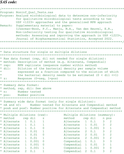
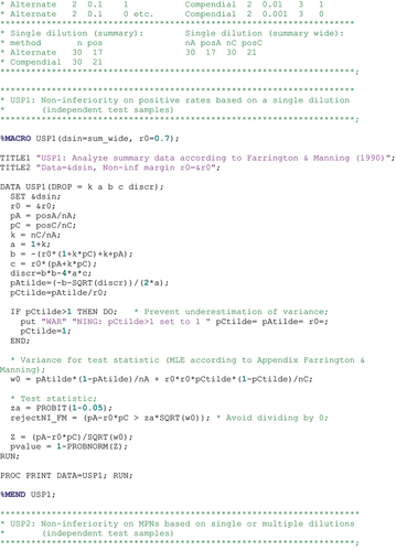
Assuming independence between the samples, simulation results were generated by drawing the true number of organisms in each sample from a Poisson distribution with mean $\lambda$ for a single dilution, and $\lambda$ divided by the appropriate dilution factor for samples from a dilution series. The detection probability for each sample was then calculated using formula (7), and the outcome of the sample was positive if this probability was larger than a random number between 0 and 1, and negative otherwise. The simulated data were analyzed using the different approaches USP1, USP2, and gMPN. SAS and R codes for such analyses are presented in Appendix 2. For the USP2 approach, MPN replicates sometimes failed. In those cases, the MPN for the alternative and/or the compendial method could not be estimated because all samples in all dilutions were positive or negative for that method. In simulations where this occurred, the t-test was calculated based on the remaining MPN replicates, as one would usually do in practice. For all three methods, the Type I error and power were estimated by the percentage of simulations for which non-inferiority was concluded. Failure rates were estimated by the percentage of MPN replicates for which all samples were positive (all samples negative did not occur) out of the total number of MPN replicates across all simulations. Note that the expected failure percentages can also be calculated theoretically based on formula (8). For example, for a 3 × $k$ design with spike levels ${\lambda }_1$, ${\lambda }_2$, and ${\lambda }_3$, this would be $100\cdot \prod _{i=1}^3{\left(1-\mathrm{e}\mathrm{x}\mathrm{p}\left(-\theta {\lambda }_i\right)\right)}^k$.

6. Results

First, we compared USP1 and gMPN on their Type I error rates. Table 2 shows the expected Type I error rates of around 5% for the gMPN approach, but unacceptably high Type I errors for USP1. These Type I errors increase rapidly with the spike level up to almost 100% when λ$\ge 3$, which means that the USP1 approach based on the positive rates almost always concludes non-inferiority, while in fact the alternative method detects one organism with a probability of only 80% of that of the compendial method, which is exactly equal to the selected non-inferiority margin. Also when the ratio of detection proportions is chosen below the non-inferiority margin of 0.8 (${\theta }_A=0.7{\theta }_C=0.56$), USP1 still shows rapidly increasing probabilities beyond 5% when the spike level increases from 1.5 to above (Appendix 3, Table C1), while the gMPN shows probabilities below nominal (as expected). The last two columns in Table 2 show that when the ratio of positive rates equals the non-inferiority margin (which can only occur at one specific spike level), the Type I error of USP1 is around 5%. The ratio of detection proportions is then already far below the non-inferiority margin of 0.8 and the gMPN shows Type I errors below nominal.

Table 2. Type I error rate (%) to conclude non-inferiority with approaches USP1 and gMPN for a single dilution design using a non-inferiority margin of $r_0=0.8$, detection proportion ${\theta }_C=0.8$, ${\theta }_A$ chosen such that ${\theta }_A/{\theta }_C=r_0$ or $p_A/p_C=r_0$, and $n=200$ samples.

Density λ	0.5	1.0	1.5	2.0	2.5	3.0	2.0	3.0
Detection proportion ${\theta }_A$	0.64						0.509	0.433
${\theta }_A/{\theta }_C$	0.80						0.636	0.542
Expected positive rates (%)$p_A$	27.39	47.27	61.71	72.20	79.81	85.34	63.85	72.74
$p_C$	32.97	55.07	69.88	79.81	86.47	90.93	79.81	90.93
$p_A/p_C$	0.831	0.858	0.883	0.905	0.923	0.939	0.80
USP1	8.3	17.9	38.8	67.6	91.4	99.1	5.2	5.4
gMPN	5.1	5.4	4.8	5.4	5.0	4.7	0.0	0.0

Table 3 shows for the same single dilution design the power for non-inferiority when the detection proportions of the alternate and compendial method are equal (${\theta }_A={\theta }_C=0.8$). With 200 samples per method, the powers for USP1 are very high (over 95% for spike levels of λ$=1.5$ or higher), but we know that this is at the cost of highly inflated Type I errors. For the gMPN method, the power using a non-inferiority margin of $r_0=0.8$ attains a maximum value of about 57% for λ$\approx 2$. To increase the power, one should either test even more samples than $n=200$ per method or relax the non-inferiority margin. When a margin of $r_0=0.7$ instead of $r_0=0.8$ would be applied, then the power for the gMPN approach would be sufficient, with a maximum value of 89% for the optimal spike level, and still values above 80% when the average spike level is between 1 and 3. Please note that other values than 0.8 for the equal detection proportions would have led to similar results at slightly different spike levels, since results are driven by the product $\xi =\theta \lambda$ in formula (8). Appendix 3, Tables C2 and C3 show results for the power when detection proportions differ, i.e. for $\left({\theta }_A,{\theta }_C\right)=\left(0.72,0.8\right)$ or $\left(0.88,0.8\right).$ Apart from the powers being lower or higher, respectively, than for $\left({\theta }_A,{\theta }_C\right)=\left(0.8,0.8\right)$, the pattern is the same.

Table 3. Power (%) to conclude non-inferiority with approaches USP1 and gMPN for a single dilution design using a non-inferiority margin of $r_0=0.8$ or $r_0=0.7$, detection proportions $\left({\theta }_A,{\theta }_C\right)=\left(0.8,0.8\right)$ and $n=200$ samples.

Density	λ		0.5	1.0	1.5	2.0	2.5	3.0
Expected positive rates (%)	$p_A=p_C$		32.97	55.07	69.88	79.81	86.47	90.93
Non-inferiority margin	$r_0=0.8$	USP1	46.8	79.1	95.2	99.6	100.0	100.0
		gMPN	35.0	48.4	54.8	57.2	53.3	52.2
	$r_0=0.7$	USP1	79.7	98.6	100.0	100.0	100.0	100.0
		gMPN	64.2	82.2	86.6	88.7	87.6	85.0

To evaluate the second USP approach, which uses a t-test on a set of estimated MPNs, we simulated multiple dilution designs and compared the Type I error and the power of USP2 with that of the gMPN approach. Table 4 shows that the Type I error rates for a detection proportion ratio at the non-inferiority margin of 0.8 (${\theta }_A=r_0{\theta }_C=0.64$) are all close to the nominal 5% level for the gMPN approach, while for the USP2 approach they are in most cases smaller and below 4.5%. Only for dilution factor 2 in the 3 × 3, 3 × 4 and 3 × 5 designs, the Type I error for the USP2 approach is somewhat inflated, probably because of the higher number of failed MPN replicates in the compendial than in the alternative group, leading to elimination of the MPN replicates for which the compendial method had all samples positive. All failure rates were in line with the theoretical expected value. For a ratio of detection proportions below the non-inferiority margin (${\theta }_A=0.7{\theta }_C=0.56$), probabilities for both USP2 and gMPN are below the nominal 5% level, but the pattern is the same (Appendix 3, Table C4).

Table 4. Type I error rate (%) to conclude non-inferiority with approaches USP2 and gMPN for multiple dilution designs using a non-inferiority margin of $r_0=0.8$, detection proportions $\left({\theta }_A,{\theta }_C\right)=\left(0.64,0.8\right)$ and n~200 samples.

Design			$r_0=0.8$		Failed MPNs (%) for USP2
n~200	$n$	λ	USP2	gMPN	Alternative	Compendial
3 × 3 × 22	198	4,2,1	6.8	4.9	6,843 (3.1)	16,384 (7.4)
3 × 4 × 16	192		5.2	5.0	1,521 (1.0)	5,028 (3.1)
3 × 5 × 13	195		4.5	5.0	421 (0.3)	1,712 (1.3)
3 × 6 × 11	198		4.1	4.6	126 (0.1)	590 (0.5)
3 × 7 ×  9	189		4.3	5.0	35 (0.0)	225 (0.3)
3 × 8 ×  8	192		4.5	4.8	4 (0.0)	89 (0.1)
3 × 11 × 6	198		4.4	4.9	-	2 (0.0)
3 × 13 × 5	195		4.5	5.1	-	-
3 × 16 × 4	192		4.3	5.1	-	-
3 × 22 × 3	198		3.5	5.0	-	-
3 × 33 × 2	198		2.8	5.0	-	-
3 × 3 × 22	198	20,2,0.2	3.8	4.8	133 (0.1)	373 (0.2)
3 × 4 × 16	192		3.9	5.1	7 (0.0)	31 (0.0)
3 × 5 × 13	195		3.7	4.9	1 (0.0)	2 (0.0)
3 × 6 × 11	198		3.9	4.9	-	1 (0.0)
3 × 7 ×  9	189		4.1	4.8	-	-
3 × 8 ×  8	192		4.2	4.9	-	-
3 × 11 × 6	198		4.2	5.0	-	-
3 × 13 × 5	195		4.6	5.3	-	-
3 × 16 × 4	192		4.5	5.4	-	-
3 × 22 × 3	198		4.1	5.3	-	-
3 × 33 × 2	198		2.7	5.1	-	-

Results in Table 5 show that the power for gMPN is stable across the different designs. For USP2 with dilution factor 2, the power seems to decrease with a decreasing number of replicates, while it is stable for dilution factor 10, until the number of replicates drops below 5. This may be due to a low number of degrees of freedom that is then used in the t-test. Note that for dilution factor 2, more failures occurred than for dilution factor 10, since the different dilutions are more likely to have only positives if they are closer together. The failure rate also decreases when the number of samples per dilution increases, since it becomes more difficult for a replicate to fail, i.e. to have all samples in all dilutions positive. Except for the 3 × 3 × 22 design with dilution factor 2, the power for USP2 is always smaller than for gMPN. A reason for USP2 having lower power than gMPN is most likely that USP2 compares multiple (depending on the number of replicates 22, 16, etc.) MPN estimates between the two methods but does not use the precision of the MPN estimates themselves, while the gMPN approach uses all data together without discarding or losing information.

Table 5. Power (%) to conclude non-inferiority with approaches USP2 and gMPN for multiple dilution designs using a non-inferiority margin of $r_0=0.8$ or $r_0=0.7$, detection proportions $\left({\theta }_A,{\theta }_C\right)=\left(0.8,0.8\right)$ and n~200 samples.

Design		$r_0=0.8$		$r_0=0.7$		Failed MPNs (%) for USP2
n~200	λ	USP2	gMPN	USP2	gMPN	Alternative	Compendial
3 × 3 × 22	4,2,1	50.8	49.2	84.4	83.1	16,643 (7.6)	16,384 (7.4)
3 × 4 × 16		44.9	47.2	79.2	81.6	4,949 (3.1)	5,028 (3.1)
3 × 5 × 13		43.3	48.7	77.0	82.1	1,720 (1.3)	1,712 (1.3)
3 × 6 × 11		42.9	48.7	75.7	82.8	655 (0.6)	590 (0.5)
3 × 7 ×  9		41.2	47.2	73.7	80.9	229 (0.3)	225 (0.3)
3 × 8 ×  8		41.9	48.0	73.9	81.7	87 (0.1)	89 (0.1)
3 × 11 × 6		41.5	48.8	74.7	83.4	4 (0.0)	2 (0.0)
3 × 13 × 5		40.2	49.4	71.7	82.4	-	-
3 × 16 × 4		37.2	47.4	68.0	81.8	-	-
3 × 22 × 3		32.3	50.0	60.8	83.1	-	-
3 × 33 × 2		17.9	49.1	33.5	82.4	-	-
3 × 3 × 22	20,2,0.2	25.5	30.9	47.0	57.3	352 (0.2)	373 (0.2)
3 × 4 × 16		24.4	30.0	44.8	55.0	23 (0.0)	31 (0.0)
3 × 5 × 13		25.0	30.4	46.9	57.1	5 (0.0)	2 (0.0)
3 × 6 × 11		25.4	30.7	46.6	56.3	-	1 (0.0)
3 × 7 ×  9		24.2	29.6	46.0	56.1	-	-
3 × 8 ×  8		25.0	30.0	45.9	55.7	-	-
3 × 11 × 6		25.5	31.9	47.7	57.0	-	-
3 × 13 × 5		25.3	31.7	46.3	57.4	-	-
3 × 16 × 4		22.8	30.9	42.6	55.9	-	-
3 × 22 × 3		20.4	31.8	37.7	57.5	-	-
3 × 33 × 2		11.4	31.0	20.2	56.8	-	-

Comparing the gMPN results of Table 5 with Table 3 shows that the power for a single dilution experiment with a close to optimal spike level is higher than for a multiple dilution experiment, which includes only part of the data at the optimal spike level. Diluting further away from the optimal spike level decreases the power for both methods, which is also clear when comparing dilution factor 10 with dilution factor 2. Also, designs with five dilutions (not shown) would have lower power than designs with three dilutions.

Using a non-inferiority margin of $r_0=0.7$ instead of $r_0=0.8$ would, with a dilution factor of 2, be sufficient to increase the power to values above 80% for gMPN and USP2 with the 3 × 3 × 22 design, but not for USP2 with the other designs with less replicates.

Appendix 3, Tables C5 and C6 show results for the power when detection proportions differ, i.e. for $\left({\theta }_A,{\theta }_C\right)=\left(0.72,0.8\right)$ or $\left(0.88,0.8\right).$ Apart from the powers being lower or higher, respectively, than for $\left({\theta }_A,{\theta }_C\right)=\left(0.8,0.8\right)$, the pattern is the same.

7. Conclusions

This paper presented the two USP <1223> non-inferiority approaches (USP1 on positive rates, USP2 on MPNs) and a statistical model that helped to interpret these approaches and that led to a third approach (generalized MPNs). Simulations illustrated the performance of the three approaches. It can be concluded that USP1 on positive rates is not suitable, since it concludes non-inferiority too often when the alternate method is inferior in detecting a single organism. This becomes even more severe for higher spike levels (already at 2–3 CFU/sample, which is still far below the spike level of 10–50 CFU that USP suggests), for which the expected positive rates become closer to 100% and closer to each other. Obviously, for sufficiently high spike levels, also a poor method has no difficulty detecting positive samples. Hence, the positive rate is not a good measure to evaluate the method performance, since it is influenced not only by the method but also by the spike level, and the conclusion of non-inferiority would only hold for the spike level tested, which cannot be estimated. Even if one would consider non-inferiority on the positive rates from a certain spike level onwards sufficient, then the spiking uncertainty in microbiology and the fact that the power changes rapidly with the spike level, make it very difficult to set up an experiment that guarantees this. Due to this dependence on the spike level, there is also no easy way to choose a lower significance level to get the Type I error under control, in an attempt to still benefit from the increase in power.

On the other hand, USP2 is a suitable approach to evaluate the sensitivity of the alternative method in comparison with the compendial method and is not driven by the spike level. However, the proposed set-up for MPN can be improved. Instead of using multiple dilutions, it would be better to use the optimal single spike level that maximizes the power of the test. Under realistic scenarios with detection proportions above 0.7, the optimal spike level would be approximately 2 CFU/sample (for more details, see IJzerman-Boon and Van den Heuvel 2015; Strijbosch et al. 1990). If multiple dilutions are used, for example, to mitigate the risk of spiking uncertainty, then a much smaller dilution factor should be used in order to stay as close as possible to the optimal spike level. Moreover, it is recommended to use as many MPN replicates as possible, but 3 × 3 or 3 × 4 experiments are not recommended due to the high probability of failed MPN replicates, which could lead to a bias in the evaluation.

An even better alternative is to replace the t-test by the generalized MPN analysis, i.e. to use gMPN instead of USP2. The MPN approach ignores the variability of the individual MPN estimates, which is overcome in an analysis of all data simultaneously by the gMPN. Use of all data together generally increases the power and reduces the risk of failed MPN replicates in the MPN experiment. Furthermore, the sample size of 75–100 that USP <1223> suggests for 80–90% power should be increased to about 200, since lower sample sizes do not provide this power level, not even when the non-inferiority margin is 0.7. To mitigate this increase in sample size, one may consider analyzing the data of multiple organisms together, provided their ratios of detection proportions are homogeneous (Emampour et al. 2021).

In the simulations, we assumed that the true counts in the samples were independent Poisson. This is a theoretical assumption for the estimation of MPNs in USP2 as well as for the ratio of detection proportions ${\hat{\theta }}_A/{\hat{\theta }}_C$ in gMPN. It is not a serious drawback, since in practice it may always be approximately achieved by making sure that the volumes taken for the dilutions are small compared to the stock solution, and that the test samples are small compared to the dilutions. However, if samples are not independent Poisson, then the different ways of executing MPN experiments (Figure 2) may play a role, and taking into account some pairing in the analysis, using the USP2 paired MPN t-test, may become better than the gMPN approach, which currently ignores any dependence between the samples. This requires further investigation. For a single dilution design, the gMPN approach may still be used, but it may be best to completely divide the stock solution over the test samples, because in that case, the estimator based on Poisson is robust against under- or overdispersion (Manju et al. 2019).

One of the limitations of the gMPN approach, which also applies to the USP methods, is that we did not consider false positives in our model. If false positives are ignored, then they may compensate for false negatives, and non-inferiority may be concluded while in fact the alternate method has a lower sensitivity than the compendial in combination with false positives. This may be easily resolved, since IJzerman-Boon and Van den Heuvel (2015) presented a zero-deflated binomial detection model, which extends the binomial model (7) with a parameter for the false positive rate. Use of this extended model slightly changes formulas (8), (9), and (10), but would allow a clean comparison of the sensitivity of two methods without interference by false positives.

In conclusion, the generalized MPN approach clearly outperforms the two USP approaches with a clear interpretation under the binomial-Poisson model that we presented. Non-inferiority on the positive rates is strongly discouraged. Furthermore, the robustness of the MPN and gMPN approach against other detection probability models must still be investigated.

Disclosure statement

No potential conflict of interest was reported by the author(s).

Additional information

Funding

This work is part of the research program Rapid Micro Statistics with project number 15990, which is (partly) financed by the Dutch Research Council (NWO).

Appendix 1:

Proof that all samples are independent

Theorem

Suppose the number of organisms in the stock solution follows a Poisson distribution: $N$ ~$Poi\left(\lambda \right)$. Assume that this stock solution is split into $n$ equal samples with numbers of organisms $X_1,X_2,\dots ,X_n$. Conditional on the total number of organisms $N$ in the stock solution, the numbers in the samples follow a multinomial distribution, with probabilities $1/n$ for each organism to end up in one of the samples: $X_1,X_2,\dots ,X_n|N$~$Mult\left(N;1/n,\dots ,1/n\right)$.

Let $Z_1,Z_2,\dots ,Z_n\in \left\{0,1\right\}$ denote the test outcome for each sample ($0=$ negative, $1=$ positive). Assume that each sample is tested with a test method that detects organisms according to binomial detection model (7) with detection proportion ${\theta }_i$, which may differ for each sample $i=1,\dots ,n$: $P\left(Z_i=1|X_i\right)=1-{\left(1-{\theta }_i\right)}^{X_i}$.

Then:

1. the true numbers of organisms $X_1,X_2,\dots ,X_n$ in the test samples follow an independent Poisson distribution, with marginal distribution: $X_1,X_2,\dots ,X_n$~$Poi\left(\lambda /n\right)$.

2. the positive/negative test results $Z_1,Z_2,\dots ,Z_n$ are independent with Bernoulli probabilities: $P\left(Z_i=1\right)=1-\mathrm{e}\mathrm{x}\mathrm{p}\left(-{\theta }_i\lambda /n\right)$, or equivalently, $P\left(Z_i=0\right)=\mathrm{e}\mathrm{x}\mathrm{p}\left(-{\theta }_i\lambda /n\right)$.

Proof

(a) This follows from Theorem 1 and its Corollary 4 in Section 4 (about mixtures on the total number ($N$) of the multinomial distribution) of Patil and Bildikar (1966).

(b) In order to prove independence, i.e. that for all $z_1,\dots ,z_n\in \left\{0,1\right\}$

$P\left(Z_1=z_1,\dots ,Z_n=z_n\right)=P\left(Z_1=z_1\right)\cdot \dots \cdot P\left(Z_n=z_n\right),$

it is sufficient to prove that:

(A1) $P\left(Z_1=0,\dots ,Z_n=0\right)=P\left(Z_1=0\right)\cdot \dots \cdot P\left(Z_n=0\right),$(A1)

since the occurrence of 0 and 1 are complementary events, and for events $A_1,\dots ,A_n$, independence of the events themselves also implies independence when one or more of the events is replaced by its complementary event, i.e.

$P\left(A_1,\dots ,A_n\right)=\prod _{i=1}^{n}P\left(A_i\right)$ implies $P\left(A_1^c,A_2,\dots ,A_n\right)=P\left(A_1^c\right)\prod _{i=2}^{n}P\left(A_i\right)$,

since we can write

$P\left(A_1^c,A_2,\dots ,A_n\right)=P\left(A_1^c|A_2,\dots ,A_n\right)P\left(A_2,\dots ,A_n\right)=$

$=\left[1-P\left(A_1|A_2,\dots ,A_n\right)\right]P\left(A_2,\dots ,A_n\right)=$

$=\left[1-\frac{P\left(A_1,A_2,\dots ,A_n\right)}{P\left(A_2,\dots ,A_n\right)}\right]P\left(A_2,\dots ,A_n\right)=$

$=P\left(A_2,\dots ,A_n\right)-P\left(A_1,A_2,\dots ,A_n\right)=$

$=\left[1-P\left(A_1\right)\right]\prod _{i=2}^{n}P\left(A_i\right)=$

$=P\left(A_1^c\right)\prod _{i=2}^{n}P\left(A_i\right).$

On the left-hand side of (A1), we have

$P\left(Z_1=0,\dots ,Z_n=0\right)=$

$=\sum _{N=0}^{\mathrm{\infty }}\sum _{\begin{array}{c}{ }_{x_1=0}\\ {}_{x_1+\dots +x_n=N}\end{array}}^N\dots \sum _{x_n=0}^{N}P\left(Z_1=0,\dots ,Z_n=0|X_1=x_1,\dots ,X_n=x_n,N=N\right)\cdot$

$\cdot P(X_1=x_1,\dots ,X_n=x_n|N=N)\cdot P\left(N=N\right)=$

($\left(Z_i|X_1,\dots ,X_n,N\right)$ are conditionally independent therefore this is just the product)

$=\sum _{N=0}^{\mathrm{\infty }}\sum _{x_1=0}^N\dots \sum _{x_n=0}^N\left[\prod _{i=1}^{n}P\left(Z_i=0|X_1=x_1,\dots ,X_n=x_n,N=N\right)\right]\cdot$

$\cdot P(X_1=x_1,\dots ,X_n=x_n|N=N)\cdot P\left(N=N\right)=$

(if we know $X_i$, then the other $X$’s do not matter, whether they are independent or not)

$=\sum _{N=0}^{\mathrm{\infty }}\sum _{x_1=0}^N\dots \sum _{x_n=0}^N\left[\prod _{i=1}^{n}P\left(Z_i=0|X_i=x_i\right)\right]\cdot P\left(X_1=x_1,\dots ,X_n=x_n|N=N\right)\cdot P\left(N=N\right)=$

$=\sum _{N=0}^{\mathrm{\infty }}\sum _{x_1=0}^N\dots \sum _{x_n=0}^N\left[\prod _{i=1}^n{\left(1-{\theta }_i\right)}^{x_i}\right]\cdot \frac{N!}{x_1!\dots x_n!}{\left(\frac{1}{n}\right)}^N\cdot \frac{{\lambda }^N{e}^{-\lambda }}{N!}=$

(multinomial theorem ${\left(a_1+\dots +a_n\right)}^N=\sum _{x_1+\dots +x_n=N}^{\hspace{0.17em}}\left(\begin{array}{c}N\\ x_1,\dots ,x_n\end{array}\right)a_1^{x_1}\dots a_n^{x_n}$)

$=\sum _{N=0}^{\mathrm{\infty }}{\left(n-{\theta }_1-\dots -{\theta }_n\right)}^N{\left(\frac{1}{n}\right)}^N\cdot \frac{{\lambda }^N{e}^{-\lambda }}{N!}=$

(Poisson distribution $Poi\left(\left(1-\sum _{i=1}^n{\theta }_i/n\right)\lambda \right)$ adds up to 1 over all $N$)

$=\sum _{N=0}^{\mathrm{\infty }}\frac{{\left(\left(1-{\sum }_{i=1}^n{\theta }_i/n\right)\lambda \right)}^N{e}^{-\lambda \left(1-{\sum }_{i=1}^n{\theta }_i/n\right)+\lambda \left(1-{\sum }_{i=1}^n{\theta }_i/n\right)-\lambda }}{N!}=$

$=1\cdot e^{\lambda \left(1-\sum _{i=1}^n{\theta }_i/n\right)-\lambda }=e^{-\lambda \sum _{i=1}^n{\theta }_i/n}.$

On the right-hand side of (A1), we have for $Z_1$ and similarly for $Z_2,\dots ,Z_n$

$P\left(Z_1=0\right)=\sum _{N=0}^{\mathrm{\infty }}\sum _{\begin{array}{c}{ }_{x_1=0}\\ { }_{x_1+\dots +x_n=N}\end{array}}^N\dots \sum _{x_n=0}^{N}P\left(Z_1=0|X_1=x_1,\dots ,X_n=x_n,N=N\right)\cdot$

$\cdot P\left(X_1=x_1,\dots ,X_n=x_n|N=N\right)\cdot P\left(N=N\right)=$

($Z_1$ only depends on $X_1$)

$=\sum _{N=0}^{\mathrm{\infty }}\sum _{x_1=0}^N\dots \sum _{x_n=0}^{N}P\left(Z_1=0|X_1=x_1\right)\cdot P\left(X_1=x_1,\dots ,X_n=x_n|N=N\right)\cdot P\left(N=N\right)=$

$=\sum _{N=0}^{\mathrm{\infty }}\sum _{x_1=0}^N\dots \sum _{x_n=0}^N{\left(1-{\theta }_1\right)}^{x_1}\cdot \frac{N!}{x_1!\dots x_n!}{\left(\frac{1}{n}\right)}^N\cdot \frac{{\lambda }^N{e}^{-\lambda }}{N!}=$

$=\sum _{N=0}^{\mathrm{\infty }}\sum _{x_1=0}^N\dots \sum _{x_n=0}^N{\left(1-{\theta }_1\right)}^{x_1}\cdot \frac{N!}{x_1!\left(N-x_1\right)!}\frac{\left(N-x_1\right)!}{x_2!\dots x_n!}{\left(\frac{1}{n}\right)}^N\cdot \frac{{\lambda }^N{e}^{-\lambda }}{N!}=$

$=\sum _{N=0}^{\mathrm{\infty }}\sum _{x_1=0}^N{\left(1-{\theta }_1\right)}^{x_1}\cdot \frac{N!}{x_1!\left(N-x_1\right)!}\sum _{x_2=0}^{N-x_1}\dots \sum _{x_n=0}^{N-x_1}\frac{\left(N-x_1\right)!}{x_2!\dots x_n!}{\left(\frac{1}{n-1}\right)}^{N-x_1}{\left(\frac{n-1}{n}\right)}^{N-x_1}{\left(\frac{1}{n}\right)}^{x_1}\cdot \frac{{\lambda }^N{e}^{-\lambda }}{N!}=$

(multinomial distribution $Multin\left(N-x_1;\frac{1}{n-1},\dots ,\frac{1}{n-1}\right)$ adds up to 1)

$=\sum _{N=0}^{\mathrm{\infty }}\sum _{x_1=0}^N\frac{N!}{x_1!\left(N-x_1\right)!}\cdot 1\cdot {\left(\frac{n-1}{n}\right)}^{N-x_1}{\left(\frac{1-{\theta }_1}{n}\right)}^{x_1}\cdot \frac{{\lambda }^N{e}^{-\lambda }}{N!}=$

(Newton’s binomium ${\left(a+b\right)}^N=\sum _{x=0}^N\left(\begin{array}{c}N\\ x\end{array}\right)a^x{b}^{N-x}$)

$=\sum _{N=0}^{\mathrm{\infty }}{\left(\frac{1-{\theta }_1}{n}+\frac{n-1}{n}\right)}^N\cdot \frac{{\lambda }^N{e}^{-\lambda }}{N!}=$

(Poisson distribution $Poi\left(\left(1-{\theta }_1/n\right)\lambda \right)$ adds up to 1 over all $N$)

$=\sum _{N=0}^{\mathrm{\infty }}\frac{{\left(\left(1-{\theta }_1/n\right)\lambda \right)}^N{e}^{-\lambda \left(1-{\theta }_1/n\right)+\lambda \left(1-{\theta }_1/n\right)-\lambda }}{N!}=e^{-\lambda {\theta }_1/n}.$

Hence, the left-hand side $P\left(Z_1=0,\dots ,Z_n=0\right)=e^{-\lambda \sum _{i=1}^n{\theta }_i/n}$equals the right-hand side $P\left(Z_1=0\right)\cdot \dots \cdot P\left(Z_n=0\right)=\prod _{i=1}^n{e}^{-\lambda {\theta }_i/n}$, thereby completing the proof.

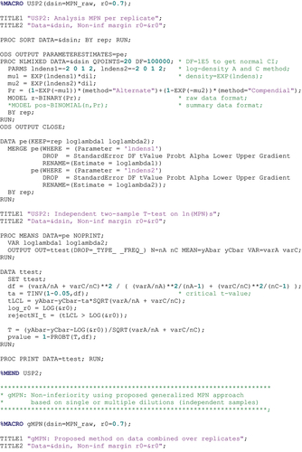
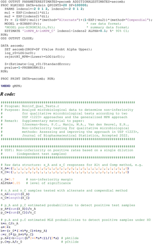
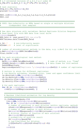
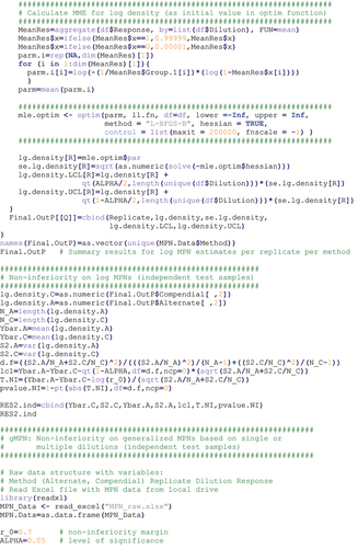
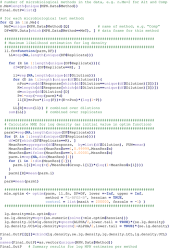
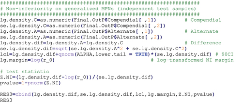
Appendix 2

Program codes for analysis

Appendix 3

Additional simulation results

Simulations supplementing those in Table 2 (Type I error USP1 vs gMPN)

Simulations supplementing those in Table 3 (Power USP1 vs gMPN)

Simulations supplementing those in Table 4 (Type I error USP2 vs gMPN)

Simulations supplementing those in Table 5 (Power USP2 vs gMPN)

Table C1. Type I error rate (%) to conclude non-inferiority with approaches USP1 and gMPN for a single dilution design using a non-inferiority margin of $r_0=0.8$, detection proportion ${\theta }_C=0.8$, ${\theta }_A$ chosen such that ${\theta }_A/{\theta }_C=0.7<r_0$, and $n=200$ samples.

Density	λ	0.5	1.0	1.5	2.0	2.5	3.0
Detection proportion	${\theta }_A$	0.56
	${\theta }_A/{\theta }_C$	0.70
Expected positive rates (%)	$p_A$	24.42	42.88	56.83	67.37	75.34	81.36
	$p_C$	32.97	55.07	69.88	79.81	86.47	90.93
	$p_A/p_C$	0.741	0.779	0.813	0.844	0.871	0.895
USP1		1.8	3.0	7.7	21.4	51.5	83.0
gMPN		0.8	0.6	0.4	0.4	0.3	0.4

Table C2. Power (%) to conclude non-inferiority with approaches USP1 and gMPN for a single dilution design using a non-inferiority margin of $r_0=0.8$ or $r_0=0.7$, ${\theta }_A/{\theta }_C=0.9$ with detection proportions $\left({\theta }_A,{\theta }_C\right)=\left(0.72,0.8\right)$ and $n=200$ samples.

Density	λ		0.5	1.0	1.5	2.0	2.5	3.0
Expected positive rates (%)	$p_A$		30.23	51.32	66.04	76.31	83.47	88.47
	$p_C$		32.97	55.07	69.88	79.81	86.47	90.93
	$p_A/p_C$		0.917	0.932	0.945	0.956	0.965	0.973
Non-inferiority margin	$r_0=0.8$	USP1	24.2	49.5	76.9	94.5	99.4	100.0
		gMPN	16.6	21.6	23.4	25.1	23.0	22.9
	$r_0=0.7$	USP1	56.7	90.7	99.5	100.0	100.0	100.0
		gMPN	39.6	56.2	61.7	64.5	64.1	60.6

Table C3. Power (%) to conclude non-inferiority with approaches USP1 and gMPN for a single dilution design using a non-inferiority margin of $r_0=0.8$ or $r_0=0.7$, ${\theta }_A/{\theta }_C=1.1$ with detection proportions $\left({\theta }_A,{\theta }_C\right)=\left(0.88,0.8\right)$ and $n=200$ samples.

Density	λ		0.5	1.0	1.5	2.0	2.5	3.0
Expected positive rates (%)	$p_A$		35.60	58.52	73.29	82.80	88.92	92.86
	$p_C$		32.97	55.07	69.88	79.81	86.47	90.93
	$p_A/p_C$		1.080	1.063	1.049	1.037	1.028	1.021
Non-inferiority margin	$r_0=0.8$	USP1	68.9	94.3	99.6	100.0	100.0	100.0
		gMPN	57.5	75.2	81.5	82.7	79.9	77.2
	$r_0=0.7$	USP1	92.6	99.9	100.0	100.0	100.0	100.0
		gMPN	83.2	95.0	97.2	97.7	97.1	95.5

Table C4. Type I error rate (%) to conclude non-inferiority with approaches USP2 and gMPN for multiple dilution designs using a non-inferiority margin of $r_0=0.8$, detection proportions $\left({\theta }_A,{\theta }_C\right)=\left(0.56,0.8\right)$ and $n\sim 200$ samples.

Design			$r_0=0.8$		Failed MPNs (%) for USP2
n~200	$n$	λ	USP2	gMPN	Alternative	Compendial
3 × 3 × 22	198	4,2,1	0.7	0.5	3,825 (1.7)	16,384 (7.4)
3 × 4 × 16	192		0.6	0.5	674 (0.4)	5,028 (3.1)
3 × 5 × 13	195		0.5	0.5	162 (0.1)	1,712 (1.3)
3 × 6 × 11	198		0.2	0.3	39 (0.0)	590 (0.5)
3 × 7 ×  9	189		0.5	0.5	7 (0.0)	225 (0.3)
3 × 8 ×  8	192		0.5	0.5	1 (0.0)	89 (0.1)
3 × 11 × 6	198		0.4	0.4	-	2 (0.0)
3 × 13 × 5	195		0.5	0.5	-	-
3 × 16 × 4	192		0.5	0.5	-	-
3 × 22 × 3	198		0.6	0.5	-	-
3 × 33 × 2	198		0.4	0.4	-	-
3 × 3 × 22	198	20,2,0.2	0.8	1.1	71 (0.0)	373 (0.2)
3 × 4 × 16	192		0.9	1.2	2 (0.0)	31 (0.0)
3 × 5 × 13	195		0.7	1.0	-	2 (0.0)
3 × 6 × 11	198		0.9	1.1	-	1 (0.0)
3 × 7 ×  9	189		1.0	1.2	-	-
3 × 8 ×  8	192		0.8	1.0	-	-
3 × 11 × 6	198		1.0	1.0	-	-
3 × 13 × 5	195		1.2	1.1	-	-
3 × 16 × 4	192		1.3	1.2	-	-
3 × 22 × 3	198		1.2	1.1	-	-
3 × 33 × 2	198		0.8	1.1	-	-

Table C5. Power (%) to conclude non-inferiority with approaches USP2 and gMPN for multiple dilution designs using a non-inferiority margin of $r_0=0.8$ or ${ }_0=0.7$, ${\theta }_A/{\theta }_C=0.9$ with detection proportions $\left({\theta }_A,{\theta }_C\right)=\left(0.72,0.8\right)$ and $n\sim 200$ samples.

Design		$r_0=0.8$		$r_0=0.7$		Failed MPNs (%) for USP2
n~200	λ	USP2	gMPN	USP2	gMPN	Alternative	Compendial
3 × 3 × 22	4,2,1	25.3	22.1	62.6	57.5	11,219 (5.1)	16,384 (7.4)
3 × 4 × 16		20.8	21.1	53.1	55.8	2,937 (1.8)	5,028 (3.1)
3 × 5 × 13		19.0	21.6	50.3	57.0	901 (0.7)	1,712 (1.3)
3 × 6 × 11		18.2	21.3	49.0	57.1	333 (0.3)	590 (0.5)
3 × 7 ×  9		17.6	20.5	47.3	55.1	91 (0.1)	225 (0.3)
3 × 8 ×  8		17.9	21.1	48.4	56.7	25 (0.0)	89 (0.1)
3 × 11 × 6		18.4	21.7	48.1	57.7	1 (0.0)	2 (0.0)
3 × 13 × 5		18.0	22.0	46.6	57.6	-	-
3 × 16 × 4		16.2	21.2	43.6	55.9	-	-
3 × 22 × 3		14.5	22.1	38.6	58.0	-	-
3 × 33 × 2		8.8	21.2	20.8	56.7	-	-
3 × 3 × 22	20,2,0.2	11.7	15.0	27.4	35.9	224 (0.1)	373 (0.2)
3 × 4 × 16		11.5	14.7	25.9	34.5	15 (0.0)	31 (0.0)
3 × 5 × 13		11.7	14.7	27.1	35.5	2 (0.0)	2 (0.0)
3 × 6 × 11		11.9	14.8	27.8	35.3	-	1 (0.0)
3 × 7 ×  9		11.8	14.1	26.8	34.5	-	-
3 × 8 ×  8		12.2	14.6	27.2	34.5	-	-
3 × 11 × 6		11.9	15.0	28.8	36.2	-	-
3 × 13 × 5		12.4	15.0	28.4	36.4	-	-
3 × 16 × 4		11.7	14.8	26.0	35.1	-	-
3 × 22 × 3		10.1	14.9	23.0	36.1	-	-
3 × 33 × 2		6.5	14.5	13.0	35.5	-	-

Table C6. Power (%) to conclude non-inferiority with approaches USP2 and gMPN for multiple dilution designs using a non-inferiority margin of $r_0=0.8$ or ${ }_0=0.7$, ${\theta }_A/{\theta }_C=1.1$ with detection proportions $\left({\theta }_A,{\theta }_C\right)=\left(0.88,0.8\right)$ and $n\sim 200$ samples.

Design		$r_0=0.8$		$r_0=0.7$		Failed MPNs (%) for USP2
n~200	λ	USP2	gMPN	USP2	gMPN	Alternative	Compendial
3 × 3 × 22	4,2,1	73.4	74.6	94.8	94.8	23,113 (10.5)	16,384 (7.4)
3 × 4 × 16		68.9	73.0	92.1	93.9	7,623 (4.8)	5,028 (3.1)
3 × 5 × 13		68.1	73.8	91.6	94.5	2,952 (2.3)	1,712 (1.3)
3 × 6 × 11		67.8	74.5	91.2	94.7	1,213 (1.1)	590 (0.5)
3 × 7 ×  9		65.4	72.3	89.1	94.1	453 (0.5)	225 (0.3)
3 × 8 ×  8		66.3	73.6	88.9	94.2	197 (0.2)	89 (0.1)
3 × 11 × 6		66.2	75.1	89.8	94.9	11 (0.0)	2 (0.0)
3 × 13 × 5		63.6	74.3	87.8	94.4	-	-
3 × 16 × 4		59.4	72.1	85.3	94.3	-	-
3 × 22 × 3		52.9	75.1	78.1	94.9	-	-
3 × 33 × 2		28.2	74.3	44.6	94.7	-	-
3 × 3 × 22	20,2,0.2	43.4	50.7	66.2	74.9	530 (0.2)	373 (0.2)
3 × 4 × 16		41.2	48.5	63.3	73.2	49 (0.0)	31 (0.0)
3 × 5 × 13		42.4	49.6	65.1	74.6	6 (0.0)	2 (0.0)
3 × 6 × 11		42.3	49.8	65.2	74.7	1 (0.0)	1 (0.0)
3 × 7 ×  9		40.7	48.7	63.6	73.3	-	-
3 × 8 ×  8		40.9	48.8	63.7	74.8	-	-
3 × 11 × 6		42.3	50.3	65.1	74.8	-	-
3 × 13 × 5		40.2	50.6	63.7	73.5	-	-
3 × 16 × 4		36.8	49.2	59.8	75.5	-	-
3 × 22 × 3		33.0	50.5	52.8	75.5	-	-
3 × 33 × 2		17.3	50.1	27.7	74.7	-	-

References

- Cochran, W. G. 1950. Estimation of bacterial density by means of the “most probable number”. Biometrics 6 (2):105–116. doi:10.2307/3001491.
- De Man, J. C. 1983. MPN tables, corrected. European Journal of Applied Microbiology and Biotechnology 17 (5):301–305. doi:10.1007/BF00508025.
- Emampour, M., P. C. IJzerman-Boon, M. A. Manju, and E. R. van den Heuvel. 2021. Optimal spiking experiment for non-inferiority of qualitative microbiological methods on accuracy with multiple microorganisms. Statistics in Biopharmaceutical Research. doi:10.1080/19466315.2021.2011397.
- EP. 2017. 5.1.6. Alternative methods for control of microbiological quality. In European Pharmacopeia, Vol. 9.2, 4339–4348. Strasbourg: EDQM.
- Farrington, C. P., and G. Manning. 1990. Test statistics and sample size formulae for comparative binomial trials with null hypothesis of non-zero risk difference or non-unity relative risk. Statistics in Medicine 9 (12):1447–1454. doi:10.1002/sim.4780091208.
- Garthright, W. E., and R. J. Blodgett. 1996. Confidence intervals for microbiological density using serial dilutions with MPN estimates. Biometrical Journal 38 (4):489–505. doi:10.1002/bimj.4710380415.
- Garthright, W. E., and R. J. Blodgett. 2003. FDA’s preferred MPN methods for standard, large or unusual tests, with a spreadsheet. Food Microbiology 20 (4):439–445. doi:10.1016/S0740-0020(02)00144-2.
- IJzerman-Boon, P. C., and E. R. van den Heuvel. 2015. Validation of qualitative microbiological test methods. Pharmaceutical Statistics 14 (2):120–128. doi:10.1002/pst.1663.
- Lachenbruch, P. A., and C. J. Lynch. 1998. Assessing screening tests: Extensions of McNemar’s test. Statistics in Medicine 17 (19):2207–2217. doi:10.1002/(SICI)1097-0258(19981015)17:19<2207::AID-SIM920>3.0.CO;2-Y.
- Manju, M. A., E. R. van den Heuvel, and P. C. IJzerman-Boon. 2019. A comparison of spiking experiments to estimate the detection proportion of qualitative microbiological methods. Journal of Biopharmaceutical Statistics 29 (1):30–55. doi:10.1080/10543406.2018.1452027.
- Patil, G. P., and S. Bildikar. 1966. Identifiability of countable mixtures of discrete probability distributions using methods of infinite matrices. Proceedings of the Cambridge Philosophical Society 62 (3):485–494. doi:10.1017/S030500410004010X.
- Strijbosch, L. W. G., R. J. M. M. Does, and W. Albers. 1990. Multiple-dose design and bias-reducing methods for limiting dilution assays. Statistica Neerlandica 44 (4):241–261. doi:10.1111/j.1467-9574.1990.tb01284.x.
- USP. 2015. <1223> Validation of alternative microbiological methods. In United States Pharmacopoeia, Vol. USP40-NF35, 1756–1770. Rockville, MD: U.S. Pharmacopoeial Convention.
- Van den Heuvel, E. R., and P. C. IJzerman-Boon. 2013. A comparison of test statistics for the recovery of rapid growth-based enumeration tests. Pharmaceutical Statistics 12 (5):291–299. doi:10.1002/pst.1581.