Dissecting the restricted mean time in favor of treatment

ABSTRACT

The restricted mean time in favor (RMT-IF) summarizes the treatment effect on a hierarchical composite endpoint with mortality at the top. Its crude decomposition into “stage-wise effects,” i.e., the net average time gained by the treatment prior to each component event, does not reveal the patient state in which the extra time is spent. To obtain this information, we break each stage-wise effect into subcomponents according to the specific state to which the reference condition is improved. After re-expressing the subcomponents as functionals of the marginal survival functions of outcome events, we estimate them conveniently by plugging in the Kaplan -- Meier estimators. Their robust variance matrices allow us to construct joint tests on the decomposed units, which are particularly powerful against component-wise differential treatment effects. By reanalyzing a cancer trial and a cardiovascular trial, we acquire new insights into the quality and composition of the extra survival times, as well as the extra time with fewer hospitalizations, gained by the treatment in question. The proposed methods are implemented in the rmt package freely available on the Comprehensive R Archive Network (CRAN).

KEYWORDS:

• Clinical trials
• composite endpoints
• estimands
• recurrent events
• restricted mean survival time

1. Introduction

Patients in a phase-III clinical trial often experience nonfatal events like hospitalization or relapse of disease before they die. Assessing the composite outcomes based solely on time to the first event, whichever type it is, raises concerns over the inefficient use of data as well as indiscrimination between morbidity and mortality (Anker and McMurray 2012; Armstrong and Westerhout 2017; Freemantle et al. 2003; Mao and Kim 2021). In response, investigators increasingly turn to methods that compare patients in pairs across arms, as this allows them to capture the entirety of patient data and to prioritize death over lesser events (see, e.g., Abdalla et al. 2016; Buyse 2010; Cui et al. 2022; Dong et al. 2018, 2022, 2023; Finkelstein and Schoenfeld 1999; Kandzari et al. 2021; Mao et al. 2022; Maurer et al. 2018; Pocock et al. 2012; Redfors et al. 2020; Seifu et al. 2022).

The restricted mean time in favor (RMT-IF) of treatment is one such method (Mao 2023). Defined as the net average time a treated patient fares in a more “favorable” state than an untreated one within a fixed time window, the RMT-IF has all the advantages of a pairwise comparison scheme. In addition, by pre-setting the time frame of comparison, it produces a well-defined estimand that is transferable across studies with different censoring patterns (Akacha et al. 2017; Dong et al. 2020; Oakes 2016). Furthermore, the estimand can be additively decomposed into a number of “stage-wise” effects according to the event type against which favorability is measured. Against relapse, for example, a patient gains favorable time by staying in remission; against death, by staying alive (in this case, the stage-wise effect coincides with the difference in restricted mean survival time, or RMST (McCaw et al. 2019; Royston and Parmar 2011; Tian et al. 2018; Uno et al. 2014)). Such decomposition reveals the contributions of different events to the overall effect.

Yet it may still hide important details. The stage-wise effect for survival (i.e., net RMST), for example, provides the average (treatment-conferred) extra lifetime without telling whether it is lived healthily or with illness. Similar ambiguity arises in any nonfatal event ranked above a less severe one, say, metastasis over non-metastatic relapse of cancer (Crowther and Lambert 2017). The stage-wise effect for metastasis then concerns only time spent metastasis-free, whether that means in complete remission or after relapse. Inquisition into such details requires us to further break down the stage-wise effects. While Mao (2023) alluded to the possibility of doing so, a full solution has not yet been worked out.

Another problem mentioned in the original paper but still left untreated is joint testing of the decomposed units. Although it is natural to use the estimator of the overall RMT-IF for a global test, this may not always be optimal because it hides possible variations among the components. A joint test, on the other hand, is expected to be more sensitive to component-specific deviations from the null.

In this paper, we proposed methods to further decompose the stage-wise effects to answer the kind of substantive questions raised earlier. We also develop joint tests on the stage-wise components as well as their subcomponents to provide more options for testing. We begin Section 2 by reviewing the RMT-IF and its main components with the outcomes formulated as a multistate process with hierarchically ranked states. We then introduce the subcomponents and develop estimators as well as inference procedures, with technical details relegated to the Appendix. The robust variance matrices for the main and subcomponents are then used to construct chi-square tests with multiple degrees of freedom. For both the further decomposition and joint testing, a separate strategy is designed for the special case of recurrent events and death. We also describe the usage of the R-programs that implement the new analyses. Extensive simulations are conducted in Section 3 to assess the finite-sample performance of the estimation and testing procedures. The colon cancer and heart failure trials considered in Mao (2023) are reanalyzed in Section 4 for deeper understanding of the treatment effects. We conclude the paper in Section 5 with a summary and some practical considerations.

2. Methods

2.1. Review of RMT-IF

As in Mao (2023), we use a multistate process $Y^{(a)}(t)$ to denote the composite outcomes on a generic subject from group $a$, where $a=1$ and 0 indicate the treatment and control groups, respectively. Suppose $Y^{(a)}(t)\in \{0,1,\dots ,K,\mathrm{\infty }\}$, with a larger number representing a more adverse state. In particular, states 0 and $\mathrm{\infty }$ will always represent the initial event-free status and death, respectively. Those in-between depend on the application, e.g., 1 for cancer relapse and 2 for metastasis, as shown in Figure 1 (a); or $1,\dots ,K$ for the cumulative number of a recurrent event like hospitalization, as shown in Figure 1 (b), where $K$ is the (data-dependent) maximum number of events per patient.

Figure 1. Composite endpoints formulated as multistate processes: (a) Relapse, metastasis, and death in cancer studies (Crowther and Lambert 2017); (b) Repeated hospitalizations and death in, e.g., cardiovascular trials (Vardeny et al. 2021).

With restricting time $\tau >0$, the RMT-IF estimand can be expressed as

(1) $\mu (\tau )=E\left[{\int }_0^{\tau }I\{Y^{>(1)}(t)<Y^{(0)}(t)\}\mathrm{d}t\right]-E\left[{\int }_0^{\tau }I\{Y^{(0)}(t)<\hspace{0.17em}{Y}^{(1)}(t)\}\mathrm{d}t\right],$(1)

where $Y^{(1)}(t)$ and $Y^{(0)}(t)$ are two generic outcomes independently drawn from the treatment and control groups, respectively, and $I(\cdot )$ is the indicator function. Since ${\int }_0^{\tau }I\{Y^{(a)}(t)<Y^{(1-a)}(t)\}\mathrm{d}t$ is the length of time $Y^{(a)}(\cdot )$ occupies a less severe state than $Y^{(1-a)}(\cdot )$ does in $[0,\tau ]$, the right-hand side of (1) can be interpreted as the net average time gained by the treatment in a more favorable state as compared to the control in the first, say, $\tau$ years. As with the RMST, the interpretation of the RMT-IF is tied to the choice of the restricting time.

In the comparison, we can split $\mu (\tau )$ into $(K+1)$ main components or stage-wise effects, according to the “losing” state. For example, in Figure 1 (a) where $K=2$, a favorable comparison can result from being (i) event-free (state 0) vs relapsed but non-metastatic and alive (state 1); (ii) non-metastatic and alive (states 0 or 1) vs metastatic and alive (state 2); and (iii) alive (states 0, 1, or 2) vs dead (state $\mathrm{\infty }$). More generally, write $I\{Y^{(a)}(t)<Y^{(1-a)}(t)\}={\sum }_{k=1}^{K,\mathrm{\infty }}I\{Y^{(a)}(t)<Y^{(1-a)}(t)=k\}$ (the indicators in the sum are non-overlapping). Then, by (1), it is easy to find that

$\mu (\tau )=\sum _{k=1}^{K,\mathrm{\infty }}{\mu }_k(\tau ),$

where

(2) ${\mu }_k(\tau )=E\left[{\int }_0^{\tau }I\{Y^{(1)}(t)<Y^{(0)}(t)=k\}\mathrm{d}t\right]-E\left[{\int }_0^{\tau }I\{Y^{(0)}(t)<Y^{(1)}(t)=k\}\mathrm{d}t\right].$(2)

The $k$th component ${\mu }_k(\tau )$ measures the net average time favorable with reference to state $k$. Hence, in Figure 1 (a), ${\mu }_1(\tau )$ is the net average relapse-free time (vs relapsed but non-metastatic and alive); ${\mu }_2(\tau )$ is the net average metastasis-free time (vs metastatic but alive); and ${\mu }_{\mathrm{\infty }}(\tau )$ is the net average lifetime (alive vs dead), i.e., net RMST. With recurrent events and death (Figure 1 (b)), Mao (2023) suggested using instead the aggregate measure ${\mu }_R(\tau )={\sum }_{k=1}^K{\mu }_k(\tau )$ to summarize treatment effects on the nonfatal events as a whole.

2.2. Further decomposition and estimation

Except for ${\mu }_1(\tau )$, all other ${\mu }_k(\tau )$ can be further divided. Indeed, we can do so by differentiating on the “winning” state in each ${\mu }_k(\tau )$ via $I\{Y^{(1)}(t)<Y^{(0)}(t)=k\}={\sum }_{j<k}I\{Y^{(1)}(t)=j,Y^{(0)}(t)=k\}$. This leads to

${\mu }_k(\tau )=\sum _{j<k}{\mu }_{jk}(\tau ),$

where

${\mu }_{jk}(\tau )=E\left[{\int }_0^{\tau }I\{Y^{(1)}(t)=j,Y^{(0)}(t)=k\}\mathrm{d}t\right]-E\left[{\int }_0^{\tau }I\{Y^{(0)}(t)=j,Y^{(1)}(t)=k\}\mathrm{d}t\right].$

The subcomponent ${\mu }_{jk}(\tau )$ measures the net average time improved from state $k$ to state $j$ specifically $(j<k)$. Again using Figure 1 (a) as an example, ${\mu }_{02}(\tau )$ and ${\mu }_{12}(\tau )$ are the average pre-metastasis time gained in remission and post-relapse, respectively. Likewise, ${\mu }_{0,\mathrm{\infty }}(\tau ),{\mu }_{1,\mathrm{\infty }}(\tau )$, and ${\mu }_{2,\mathrm{\infty }}(\tau )$ are the average lifetime gained in remission, post-relapse (but pre-metastasis), and post-metastasis, respectively. Clearly, the farther apart $j$ and $k$ are, the more valuable ${\mu }_{jk}(\tau )$ is per unit. In that sense, ${\mu }_{0k}(\tau ),{\mu }_{1k}(\tau ),\dots$, and ${\mu }_{k-1,k}(\tau )$ are ordered by importance, which justifies their separate analyses. Figure 2 shows this two-level decomposition of $\mu (\tau )$ diagrammatically.

Figure 2. A graphical dissection of $\mu (\tau )={\sum }_{k=1}^{K,\mathrm{\infty }}{\mu }_k(\tau )={\sum }_{k=1}^{K,\mathrm{\infty }}{\sum }_{j<k}{\mu }_{jk}(\tau )$.

The same strategy used to estimate ${\mu }_k(\tau )$ with censored data applies to the ${\mu }_{jk}(\tau )$, only with additional derivations. As in Mao (2023), suppose that $Y^{(a)}(t)$ is a progressive process in the sense that $Y^{(a)}(t)\le Y^{(a)}(s)$ for all $0\le t\le s$ (true for both examples in Figure 1). Let $T_k^{(a)}=inf\{t:Y^{(a)}(t)\ge k\}$ $(k=1,\dots ,K,\mathrm{\infty })$. Because $Y^{(a)}(t)$ is increasing, $T_k^{(a)}$ is just the first time it goes up to state $k$ or higher. In Figure 1 (a), for example, $T_1^{(a)}$ is the time to the earliest of relapse, metastasis, and death; $T_2^{(a)}$ is the time to the earlier of metastasis and death; and $T_{\mathrm{\infty }}^{(a)}$ is the time to death. Obviously, $T_1^{(a)}\le \cdots \le T_K^{(a)}\le T_{\mathrm{\infty }}^{(a)}$ (with equalities attainable in cases of “state skipping,” e.g., death without any nonfatal events). Because of progressivity, $Y^{(a)}(t)$ is completely determined by the $(K+1)$ transition times. In fact, $Y^{(a)}(t)=k$ is equivalent to $T_k^{(a)}\le t<T_{k+1}^{(a)}$ for $k=0,1,\dots ,K$ with $T_0^{(a)}\equiv 0$ and $T_{K+1}^{(a)}\equiv T_{\mathrm{\infty }}^{(a)}$, and $Y^{(a)}(t)=\mathrm{\infty }$ is equivalent to $T_{\mathrm{\infty }}^{(a)}\le t$. This means that

(3) $\mathrm{p}\mathrm{r}\{Y^{(a)}(t)=k\}=S_{k+1}^{(a)}(t)-S_k^{(a)}(t)(k=0,1,\dots ,K)\mathrm{a}\mathrm{n}\mathrm{d}\mathrm{p}\mathrm{r}\{Y^{(a)}(t)=\mathrm{\infty }\}=1-S_{K+1}^{(a)}(t),$(3)

where $S_k^{(a)}(t)=\mathrm{p}r(T_k^{(a)}>t)$ $(k=0,1,\dots ,K,K+1)$. Using ${\mu }_{j,K+1}(\tau )$ as an alias for ${\mu }_{j,\mathrm{\infty }}(\tau )$, we find that

(4) $\begin{array}{rl}& {\mu }_{jk}(\tau )={\int }_0^{\tau }\mathrm{p}\mathrm{r}\{Y^{(1)}(t)=j,Y^{(0)}(t)=k\}\mathrm{d}t-{\int }_0^{\tau }\mathrm{p}\mathrm{r}\{Y^{(0)}(t)=j,Y^{(1)}(t)=k\}\mathrm{d}t\\ & ={\int }_0^{\tau }\mathrm{p}r\{Y^{(1)}(t)=j\}\mathrm{p}\mathrm{r}\{Y^{(0)}(t)=k\}\mathrm{d}t-{\int }_0^{\tau }\mathrm{p}\mathrm{r}\{Y^{(0)}(t)=j\}\mathrm{p}\mathrm{r}\{Y^{(1)}(t)=k\}\mathrm{d}t\\ & ={\int }_0^{\tau }\{S_{j+1}^{(1)}(t)-S_j^{(1)}(t)\}\{S_{k+1}^{(0)}(t)-S_k^{(0)}(t)\}\mathrm{d}t\\ & -{\int }_0^{\tau }\{S_{j+1}^{(0)}(t)-S_j^{(0)}(t)\}\{S_{k+1}^{(1)}(t)-S_k^{(1)}(t)\}\mathrm{d}t\end{array}$(4)

for $0=j<k=1,\dots ,K,K+1$, where $S_{K+2}^{(a)}(t)\equiv 1$. The first equality in (4) follows by interchanging the expectation and integration in (2), the second by the independence of $Y^{(1)}(\cdot )$ and $Y^{(0)}(\cdot )$, and the third by (3).

In practice, the $Y^{(a)}(\cdot )$ are censored. With $C^{(a)}$ denoting the independent censoring time, we observe ${\mathcal{O}}^{(a)}\equiv \{Y^{(a)}(t):0\le t\le T_{\mathrm{\infty }}^{(a)}\wedge C^{(a)}\}$, where $b\wedge c=min(b,c)$. In parallel with the latent $Y^{(a)}(\cdot )$, we can equivalently express ${\mathcal{O}}^{(a)}$ using a sequence of censored transition times, namely, $(X_k^{(a)},{\delta }_k^{(a)})$ $(k=1,\dots ,K,K+1)$, where $X_k^{(a)}=T_k^{(a)}\wedge C^{(a)}$ and ${\delta }_k^{(a)}=I(T_k^{(a)}\le C^{(a)})$. Let $\{{\mathcal{O}}_1^{(a)},\dots ,{\mathcal{O}}_{n_a}^{(a)}\}$ denote a random $n_a$-sample of ${\mathcal{O}}^{(a)}$ and write $n=n_1+n_0$. In the absence of competing risks other than death (see, e.g., Mao 2023), we can estimate the unknown $S_k^{(a)}(t)$ in (4) by the Kaplan--Meier estimator based on the $n_a$-sample of $(X_k^{(a)},{\delta }_k^{(a)})$.

Proposition 1

Let ${\hat{S}}_k^{(a)}(t)$ denote the Kaplan–Meier estimator for $S_k^{(a)}(t)$ $(k=1,\dots ,K,K+1)$ with ${\hat{S}}_0^{(a)}(t)\equiv 0$ and ${\hat{S}}_{K+2}^{(a)}(t)\equiv 1$. Then, for $0\le j<k=1,\dots ,K,K+1$, the subcomponent ${\mu }_{jk}(\tau )$ can be consistently estimated by

${\hat{\mu }}_{jk}(\tau )={\int }_0^{\tau }\{{\hat{S}}_{j+1}^{(1)}(t)-{\hat{S}}_j^{(1)}(t)\}\{{\hat{S}}_{k+1}^{(0)}(t)-{\hat{S}}_k^{(0)}(t)\}\mathrm{d}t$

$-{\int }_0^{\tau }\{{\hat{S}}_{j+1}^{(0)}(t)-{\hat{S}}_j^{(0)}(t)\}\{{\hat{S}}_{k+1}^{(1)}(t)-{\hat{S}}_k^{(1)}(t)\}\mathrm{d}t,$

which is asymptotically normal with variance that can be robustly estimated by (12) in the Appendix.

It can be easily shown that ${\sum }_{j<k}{\hat{\mu }}_{jk}(\tau )={\hat{\mu }}_k(\tau )$, where ${\hat{\mu }}_k(\tau )$ is Mao (2023)’s estimator for ${\mu }_k(\tau )$. To derive the asymptotic normality and variance of ${\hat{\mu }}_{jk}(\tau )$, we can expand it asymptotically into a linear form (Tsiatis 2006), i.e., a sum of i.i.d. terms, using the functional delta method on the ${\hat{S}}_k^{(a)}(t)$, whose asymptotic linear forms are known (see, e.g., Corollary 3.2.1 of Fleming and Harrington 1991). Appendix A.1 lays out the details. Using these results, we can easily make inferences and construct confidence intervals for each ${\mu }_{jk}(\tau )$.

2.3. Joint tests on the components

There are several ways to test the overall treatment effect on the composite endpoint. The simplest one is to test $H_0:\mu (\tau )=0$ using the estimator $\hat{\mu }(\tau )={\sum }_{k=1}^{K,\mathrm{\infty }}{\hat{\mu }}_k(\tau )$ along with its standard error. Alternatively, one can test on the $(K+1)$ stage-wise effects jointly, i.e.,

$H_{0,\mathrm{m}\mathrm{a}\mathrm{i}\mathrm{n}}:{\mu }_1(\tau )=\cdots ={\mu }_{\mathrm{\infty }}(\tau )=0,$

or even on the $(K+1)(K+2)/2$ subcomponents, i.e.,

$H_{0,\mathrm{s}\mathrm{u}\mathrm{b}}:{\mu }_{01}(\tau )={\mu }_{02}(\tau )={\mu }_{12}(\tau )=\cdots ={\mu }_{K,\mathrm{\infty }}(\tau )=0.$

These two tests can be advantageous when treatment effect varies substantially across components.

Proposition 2 Write

${\hat{\mu }}_{\mathrm{m}\mathrm{a}\mathrm{i}\mathrm{n}}(\tau )=\{{\hat{\mu }}_1(\tau ),\dots ,{\hat{\mu }}_{\mathrm{\infty }}(\tau ){\}}^{\mathrm{T}}and{\hat{\mu }}_{\mathrm{s}\mathrm{u}\mathrm{b}}(\tau )=\{{\hat{\mu }}_{01}(\tau ),{\hat{\mu }}_{02}(\tau ),{\hat{\mu }}_{12}(\tau ),\dots ,{\hat{\mu }}_{K,\mathrm{\infty }}(\tau ){\}}^{\mathrm{T}}.$

Let ${\hat{\mathrm{\Sigma }}}_{\mathrm{m}\mathrm{a}\mathrm{i}\mathrm{n}}(\tau )$ and ${\hat{\mathrm{\Sigma }}}_{\mathrm{s}\mathrm{u}\mathrm{b}}(\tau )$ denote the robust variance matrix estimators for ${\hat{\mu }}_{\mathrm{m}\mathrm{a}\mathrm{i}\mathrm{n}}(\tau )$ and ${\hat{\mu }}_{\mathrm{s}\mathrm{u}\mathrm{b}}(\tau )$, respectively, given in Appendix A.2. Then,

(5) $\begin{array}{c}{\hat{\mu }}_{\mathrm{m}\mathrm{a}\mathrm{i}\mathrm{n}}{\left(t\right)}^T{\hat{\mathrm{\Sigma }}}_{\mathrm{m}\mathrm{a}\mathrm{i}\mathrm{n}}{\left(t\right)}^{-1}{\hat{\mu }}_{\mathrm{m}\mathrm{a}\mathrm{i}\mathrm{n}}\left(\tau \right)\stackrel{H_{0,\mathrm{m}\mathrm{a}\mathrm{i}\mathrm{n}}}{\sim }{\chi }_{K+1}^2\\ and{\hat{\mu }}_{\mathrm{s}ub}{\left(t\right)}^t{\hat{\mathrm{\Sigma }}}_{\mathrm{s}\mathrm{u}\mathrm{b}}{\left(t\right)}^{-1}{\hat{\mu }}_{\mathrm{s}\mathrm{u}\mathrm{b}}\left(\tau \right)\stackrel{H_{0,\mathrm{s}\mathrm{u}\mathrm{b}}}{\sim }{\chi }_{\left(K+1\right)\left(K+2\right)/2}^2.\end{array}$(5)

Based on the null distributions of the quadratic forms, we can easily construct chi-square tests with $(K+1)$ and $(K+1)(K+2)/2$ degrees of freedom (d.f.) to test $H_{0,\mathrm{m}\mathrm{a}\mathrm{i}\mathrm{n}}$ and $H_{0,\mathrm{s}\mathrm{u}\mathrm{b}}$, respectively.

2.4. Special case with recurrent events and death

The procedures in Sections 2.2 and 2.3 technically apply when $Y^{(a)}(t)$ represents recurrent events and death such as in Figure 1 (b). However, comparison of individual states is substantively less meaningful when those pertain to the number of occurrences of the same event. It is rarely of interest, for example, to separate out time spent having been hospitalized twice as opposed to, say, three, four, five, or more times. Coalescing the ${\mu }_{jk}(\tau )$ into a smaller set would make interpretation easier.

One way of doing so is to dichotomize between event-free (state 0) versus living with one or more events (states $1,\dots ,K$). This splits ${\mu }_{\mathrm{\infty }}(\tau )$ (net RMST) into ${\mu }_{0,\mathrm{\infty }}(\tau )$, the extra lifetime gained event-free, and ${\mu }_{1+,\mathrm{\infty }}(\tau )={\sum }_{j=1}^K{\mu }_{j,\mathrm{\infty }}(\tau )$, the extra lifetime gained having experienced at least one event. Likewise, ${\mu }_R(\tau )$ (see the end of Section 2.1) is split into ${\mu }_{0,1+}(\tau )={\sum }_{k=1}^K{\mu }_{0k}(\tau )$, the extra time gained event-free when alive, and ${\mu }_{1+,R}(\tau )={\sum }_{k=2}^K{\sum }_{j=1}^{k-1}{\mu }_{jk}(\tau )$, the extra time gained with fewer, but nonzero, nonfatal events when alive. In sum, we have that

(6) $\mu (\tau )=\underset{{\mu }_R(\tau )}{\underbrace{{\mu }_{0,1+}(\tau )+{\mu }_{1+,R}(\tau )}}+\underset{{\mu }_{\mathrm{\infty }}(\tau )}{\underbrace{{\mu }_{0,\mathrm{\infty }}(\tau )+{\mu }_{1+,\mathrm{\infty }}(\tau )}}.$(6)

Hence no matter how large $K$ is, we will always have two main components and four subcomponents. These can be estimated by aggregating the lower-level ${\hat{\mu }}_{jk}(\tau )$ introduced in Proposition 1. A computationally more efficient approach is outlined in the supplementary materials. Corresponding joint tests with 2 and 4 d.f.’s can be constructed along the lines of Proposition 2.

2.5. Software

The R-programs that implement the new procedures are integrated with the original methodology in the rmt package. Recall that the main function to fit the RMT-IF is rmtfit(), with the basic syntax

obj <- rmtfit(id, time, status, trt, type=c(“multistate”,”recurrent”))

It accepts input data in the long format, with an id variable holding the unique patient identifiers. The time and status variables contain the event times and labels of event types, respectively. With type=”multistate” (default) for standard multistate data, the value of status corresponds to the label $k$ of the state triggered by the event, except that status = 0 for censoring and status = K + 1 for death. In Figure 1 (a), for example, status = 1, 2, and 3 indicate relapse, metastasis, and death, respectively. With type=”recurrent” for recurrent-event data, status = 1 for all nonfatal events (ordered chronologically) and status = 2 for death. In addition, the trt variable contains binary indicators for the treatment against control. At this point, we do not need to specify the restricting time $\tau$. Instead, we do so when using the summary() function on the rmtfit object to extract results on the overall and stage-wise effects for a particular $\tau$, output in a similar format to Tables 2 and 3 of Mao (2023).

Table 1. Simulation results for the estimation and inference of the ${\mu }_{jk}(\tau )$.

		$\tau =1.5$					$\tau =3.0$
$\theta$	Estimand	True	Bias	SE	SEE	CP	True	Bias	SE	SEE	CP
1.0	${\mu }_{\mathrm{\infty }}(\tau )$	0	0.000	0.037	0.037	0.949	0	0.000	0.095	0.095	0.949
	${\mu }_{0,\mathrm{\infty }}(\tau )$	0	0.000	0.022	0.021	0.948	0	0.000	0.037	0.037	0.952
	${\mu }_{1,\mathrm{\infty }}(\tau )$	0	0.000	0.011	0.011	0.951	0	0.000	0.038	0.038	0.951
	${\mu }_{2,\mathrm{\infty }}(\tau )$	0	0.000	0.009	0.009	0.954	0	0.000	0.040	0.040	0.952
	${\mu }_2(\tau )$	0	0.000	0.026	0.026	0.951	0	0.000	0.052	0.052	0.948
	${\mu }_{02}(\tau )$	0	0.000	0.019	0.019	0.951	0	0.000	0.030	0.030	0.946
	${\mu }_{12}(\tau )$	0	0.000	0.010	0.010	0.951	0	0.000	0.030	0.030	0.948
	${\mu }_1(\tau )$	0	0.000	0.023	0.022	0.948	0	0.000	0.032	0.031	0.947
0.8	${\mu }_{\mathrm{\infty }}(\tau )$	0.038	0.000	0.036	0.036	0.948	0.127	$-$0.001	0.094	0.092	0.946
	${\mu }_{0,\mathrm{\infty }}(\tau )$	0.031	0.000	0.022	0.022	0.949	0.077	$-$0.001	0.040	0.039	0.948
	${\mu }_{1,\mathrm{\infty }}(\tau )$	0.005	0.000	0.010	0.010	0.950	0.035	0.000	0.037	0.036	0.947
	${\mu }_{2,\mathrm{\infty }}(\tau )$	0.002	0.000	0.008	0.008	0.954	0.015	0.000	0.037	0.036	0.948
	${\mu }_2(\tau )$	0.032	0.000	0.026	0.026	0.951	0.076	0.000	0.054	0.054	0.949
	${\mu }_{02}(\tau )$	0.029	0.000	0.019	0.019	0.951	0.059	0.000	0.032	0.032	0.950
	${\mu }_{12}(\tau )$	0.003	0.000	0.009	0.009	0.952	0.017	0.000	0.029	0.029	0.948
	${\mu }_1(\tau )$	0.034	0.000	0.023	0.023	0.952	0.055	$-$0.001	0.034	0.034	0.945

Note True is the true value; SE and SEE are the empirical standard error of ${\hat{\mu }}_{jk}(\tau )$ or ${\hat{\mu }}_k(\tau )$ and the empirical average of their standard error estimator, respectively; CP is the empirical coverage probability of the 95% confidence interval. Each scenario is based on 10,000 replicate samples of size $n=500$.

Table 2. Simulation results for the empirical type I error of different tests.

	Overall $({\chi }_1^2)$		Main $({\chi }_3^2)$		Subcomponents $({\chi }_6^2)$
$n$	$\tau =3.0$	$\tau =4.0$	$\tau =3.0$	$\tau =4.0$	$\tau =3.0$	$\tau =4.0$
200	0.058	0.056	0.062	0.061	0.039	0.057
500	0.059	0.056	0.060	0.057	0.038	0.044
1000	0.054	0.052	0.058	0.048	0.033	0.041
2000	0.052	0.052	0.053	0.053	0.038	0.039

Table 3. Analysis of the colon cancer trial using the RMT-IF (months) of combined treatment.

	$\tau =2.5$ years			$\tau =5.0$ years			$\tau =7.5$ years
	Est	SE	$p$-value	Est	SE	$p$-value	Est	SE	$p$-value
Death	0.6	0.6	0.321	3.6	1.5	0.018	7.4	2.6	0.004
vs Remission	0.8	0.5	0.108	4.1	1.4	0.003	8.1	2.3	$<$0.001
vs Relapse	$-$0.2	0.1	0.069	$-$0.5	0.3	0.150	$-$0.7	0.5	0.155
Relapse	2.1	0.4	$<$0.001	3.4	0.7	$<$0.001	4.2	0.9	$<$0.001
Overall	2.7	0.8	0.001	7.1	1.9	$<$0.001	11.6	3.0	$<$0.001

Note: Est, estimate; SE, standard error.

Now, to carry out the further decomposition, apply the new function dissect() similarly on the rmtfit object with a user-specified $\tau$, e.g., dissect(obj, tau = 3.0). To illustrate, we pick a random dataset with $n=200$ and $K=2$ in the first simulations in Section 3 and run

> obj <- rmtfit(id, time, status, trt)

> obj_sub <- dissect(obj, tau = 3.0)

> obj_sub

Call:

rmtfit. default (id = id, time = time, status = status, trt = trt)

Restricted mean time in favor of group “1” by time tau = 3:

Estimate Std.ErrZ valuePr(>|z|)

Overall 0.5988380.1899763.15220.0016206 **

Death 0.1742550.1405691.23960.2151084

vs State 00.1354880.0646622.09530.0361410 *

vs State 10.0633260.0502681.25980.2077573

vs State 2–0.0245590.054056–0.45430.6495950

State 20.2951150.0886533.32890.0008720 ***

vs State 00.2157030.0596333.61720.0002978 ***

vs State 10.0794120.0406211.95490.0505891.

State 1 (vs 0) 0.1294680.0557982.32030.0203251 *

Overall chi-square test:

X-squared = 9.55291, df = 1, p-value = 0.002;

Joint chi-square test on main components:

X-squared = 13.53824, df = 3, p-value = 0.0036;

Joint chi-square test on subcomponents:

X-squared = 20.78061, df = 6, p-value = 0.002.

The output is largely self-explanatory. In the table below the function call, the unindented lines show results for $\mu (\tau )$ and the ${\mu }_k(\tau )$, whereas the indented ones concern the subcomponents ${\mu }_{jk}(\tau )$ (check the numerical additivity of Estimate!). The entire table is available as a numeric matrix in obj_sub$tab. We also see the results of the ${\chi }_1^2$ (same as in the Overall line of the previous table), ${\chi }_{K+1}^2$, and ${\chi }_{(K+1)(K+2)/2}^2$ tests, whose $p$-values can be extracted from the trivariate vector obj_sub$pval. When we have recurrent events instead of standard multistate data, the decomposition scheme will be different according to Section 2.4, but the output will be similarly structured.

Finally, we introduce a graphic tool called “favorability plot.” Because all components of RMT-IF (and itself) are net measures of favorable and unfavorable times, a natural way to visualize them is to put the two opposing metrics side by side, as commonly seen in opinion polls of public figures or policies. To do so, use the ggrmtif() function (powered by ggplot2) directly on the dissect object, e.g.,

ggrmtif(obj_sub, unit = “months”)

This will generate a graphic that looks like Figure 5 or 6 ahead. It differs from the “bouquet plot” (Mao 2023) in that it maps out sub- as well as main components at a fixed $\tau$, rather than just the main components over a spectrum of $\tau$. We can add a state.label option to name states $0,1,\dots ,K$ in the graphic. For example, use state.label=c(“Remission”,”Relapse”) to produce the labels appearing on the left of Figure 5. For detailed usage of the rmt package, see documentation and vignettes at https://cran.r-project.org/package=rmt.

3. Simulation Studies

In this section, we consider a standard multistate process with $K=2$, as in Figure 1 (a). Simulations for recurrent events and death are described in the supplementary materials. For a generic patient in group $a$ $(a=1,0)$, use ${\tilde{T}}_1^{(a)}$, ${\tilde{T}}_2^{(a)}$, and $D^{(a)}$ to denote the latent relapse, metastasis, and death times, respectively. When ${\tilde{T}}_2^{(a)}<{\tilde{T}}_1^{(a)}$, we consider the patient to have metastasized without experiencing (non-metastatic) relapse. This leads to a progressive process with transition times $T_1^{(a)}={\tilde{T}}_1^{(a)}\wedge {\tilde{T}}_2^{(a)}\wedge D^{(a)}$, $T_2^{(a)}={\tilde{T}}_2^{(a)}\wedge D^{(a)}$, and $T_{\mathrm{\infty }}^{(a)}=D^{(a)}$. We generated the latent event times through a trivariate Gumbel--Hougaard copula model (Oakes 1989)

(7) $\mathrm{p}\mathrm{r}\left\{{\tilde{T}}_1^{(a)}>t_1,{\tilde{T}}_1^{(a)}>t_2,D^{(a)}>s\right\}=exp\left[-{\left\{{({\theta }^a{\lambda }_1{t}_1)}^{\kappa }+{({\theta }^a{\lambda }_2{t}_2)}^{\kappa }+{({\theta }^a{\lambda }_{D}s)}^{\kappa }\right\}}^{1/\kappa }\right],$(7)

where ${\lambda }_1=0.8$, ${\lambda }_2=0.4$, ${\lambda }_D=0.2$, $\kappa =2$ (producing Kendall’s concordance coefficient $1-{\kappa }^{-1}=50\mathrm{\%}$ between components; see Oakes (1989)), and $\theta >0$ is a common hazard ratio (HR) for all events. Under (7), we can use the relationship between the transition and latent event times to show that the former follow exponential distributions: $T_1^{(a)}\sim \mathrm{E}\mathrm{x}\mathrm{p}\mathrm{n}({\theta }^a{\lambda }_1^{\ast })$, $T_2^{(a)}\sim \mathrm{E}\mathrm{x}\mathrm{p}\mathrm{n}({\theta }^a{\lambda }_2^{\ast })$, and $T_3^{(a)}\sim \mathrm{E}\mathrm{x}\mathrm{p}\mathrm{n}({\theta }^a{\lambda }_D)$, where ${\lambda }_1^{\ast }=({\lambda }_1^{\kappa }+{\lambda }_2^{\kappa }+{\lambda }_D^{\kappa }{)}^{1/\kappa }$ and ${\lambda }_2^{\ast }=({\lambda }_2^{\kappa }+{\lambda }_D^{\kappa }{)}^{1/\kappa }$. These marginal distributions allow us to derive the ${\mu }_{jk}(\tau )$ as functions of $\tau$ in closed form using (4) (see supplementary materials for details). For censoring, let $C^{(a)}\sim \mathrm{U}\mathrm{n}\mathrm{i}\mathrm{f}[1,4]\wedge \mathrm{E}\mathrm{x}\mathrm{p}\mathrm{n}(0.1)$. Under this setup, the observed relapse, metastasis, and death rates are about 60%, 35%, and 20%, respectively.

We first focused on the estimation and inference of ${\mu }_{jk}(\tau )$ described in Proposition 1. With $\theta =1$ and 0.8, we generated samples of size $n=500$ with equal allocations to the treatment and control, and estimated the ${\mu }_{jk}(\tau )$ and ${\mu }_k(\tau )$ $(0=j<k=1,2,\mathrm{\infty })$ for $\tau =1.5$ and 3.0. The results are summarized in Table 1. All estimators show minimal bias, with robust standard errors closely reflecting their empirical variations. The corresponding 95% confidence intervals cover the true values at about the nominal rate. The same simulations were repeated with sample sizes $n=200,1000$, and 2000. Similar results are shown in Tables S1–S3 in the supplementary materials.

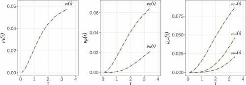
Next, we checked the accuracy of the ${\hat{\mu }}_{jk}(\tau )$ over a spectrum of $\tau$. Under $\theta =0.8$, we plotted the average estimates across $10,000$ samples generated in the previous simulations and overlaid them with the true values computed from the analytic formulas given in the supplementary materials. As seen from Figure 3, the average estimates are virtually indistinguishable from the true curves. Similar accuracy is observed for samples of size $n=200$ and $1000$ (see Figures S1 and S2 in the supplementary materials).

Figure 3. Estimation of ${\mu }_{jk}(\tau )$ as a function of $\tau$. Solid line, true values; dashed line, average estimates based on 10,000 replicates of size $n=500$.

Finally, we turned to the joint tests proposed in Section 2.3. Three types of tests were considered: a ${\chi }_1^2$ test based on $\hat{\mu }(\tau )$, a ${\chi }_3^2$ test based on the ${\hat{\mu }}_k(\tau )$, and a ${\chi }_6^2$ test based on the ${\hat{\mu }}_{jk}(\tau )$, with the latter two described in (5) of Proposition 2. Because their relative performance likely depends on the pattern of component-wise effects, we relaxed model (7) to

$\mathrm{p}\mathrm{r}\left\{{\tilde{T}}_1^{(a)}>t_1,{\tilde{T}}_1^{(a)}>t_2,D^{(a)}>s\right\}=exp\left[-{\left\{{({\theta }_1^a{\lambda }_1{t}_1)}^{\kappa }+{({\theta }_2^a{\lambda }_2{t}_2)}^{\kappa }+{({\theta }_D^a{\lambda }_{D}s)}^{\kappa }\right\}}^{1/\kappa }\right],$

where ${\theta }_1$, ${\theta }_2$, and ${\theta }_D$ are the component-specific HRs for relapse, metastasis, and death, respectively. We first checked the type I error rates of these tests with $\theta =1$, where the two groups are equivalent. All other parameters remain the same as in previous simulations. With $C^{(a)}\sim \mathrm{U}\mathrm{n}\mathrm{i}\mathrm{f}[1,6]\wedge \mathrm{E}\mathrm{x}\mathrm{p}\mathrm{n}(0.1)$, we performed level-0.05 tests at $\tau =3.0$ and $4.0$ for $n=200,500,1000$, and 2000. The empirical rejection rates are summarized across 10,000 samples in Table 2. All three tests show roughly correct type I error rate (with a slight deflation for ${\chi }_6^2$), confirming their validity.

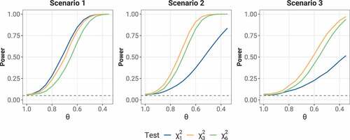
We then compared the power of these tests under alternative hypotheses. We set up three scenarios—(1) identical component-wise HR: ${\theta }_1={\theta }_2={\theta }_D=\theta$; (2) identical HR on relapse and metastasis and no effect on death: ${\theta }_1={\theta }_2=\theta$ and ${\theta }_D=1$; (3) possible effect on death but no effect on relapse or metastasis: ${\theta }_1={\theta }_2=1$ and ${\theta }_D=\theta$. In each scenario, we ran the three types of tests at $\tau =4.0$ on 10,000 replicate samples of size $n=200$ as $\theta$ decreases from 1.0 to 0.4. The resulting empirical rejection rates are plotted as a function of $\theta$ in Figure 4. When component-wise HRs are the same, ${\chi }_1^2$ is the most powerful of the three. However, it is easily outperformed by the joint tests in the latter two scenarios with heterogeneous component-wise effects.

Figure 4. Empirical power as a function of HR $\theta$ at restricting time $\tau =4.0$ based on 10,000 replicate samples of size $n=200$. Scenario 1: ${\theta }_1={\theta }_2={\theta }_D=\theta$; scenario 2: ${\theta }_1={\theta }_2=\theta$ and ${\theta }_D=1$; scenario 3: ${\theta }_1={\theta }_2=1$ and ${\theta }_D=\theta$. Dashed line, the $0.05$ significance level.

4. Real examples

With the new tools, we delve deeper into the two trials analyzed in Mao (2023) by the RMT-IF.

4.1. A colon cancer study

Moertel et al. (1990) reported a landmark colon cancer trial that established the efficacy of levamisole and fluorouracil in reducing the mortality and relapse in patients with stage C disease. The original trial involved 929 patients randomized into three arms: control $(n=304)$, levamisole alone $(n=310)$, and levamisole combined with fluorouracil $(n=315)$. Mao (2023) analyzed the data by comparing the combined treatment to the control in terms of RMT-IF, with death prioritized over relapse $(K=1)$. Over a median follow-up of 5.5 years, 119 (39%) patients in the combined treatment relapsed, 18 (5.9%) died before relapse, and 105 (34.5%) died after; 177 (56%) patients in the control relapsed, 15 (4.8%) died before relapse, and 153 (48.6%) died after. It was shown that, in the first $\tau =7.5$ years after resection of tumor (the point of randomization), the treatment on average gains the patient $\mu (\tau )=11.6$ months in a more favorable state, including an extra ${\mu }_{\mathrm{\infty }}(\tau )=7.4$ months survival time and ${\mu }_1(\tau )=4.2$ months in remission as opposed to relapse.

Following this analysis, we further examine the composition of the survival component. We consider restricting times $\tau =2.5,5.0$, and 7.5 years, and use Proposition 1 to estimate and make inferences on the subcomponents. It turns out from Table 3 that the survival benefits are fully explained by net gains in remission, which means that the prolonged life is of high quality. (The negative values of the other subcomponents are statistically insignificant and may only reflect a general reduction in relapse.) In particular, in the first $\tau =7.5$ years, treated patients on average survive 8.1 extra months in remission and lose 0.7 month post-relapse, accounting for a total of 7.4 months of net survival time. This pattern is shown in the favorability plot in Figure 5, where the between-arm imbalance in “Death vs Life” is visibly driven by “Death vs Remission”.

Figure 5. Favorability plot for the colon cancer trial at $\tau =7.5$ years.

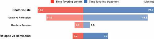
For the composite endpoint of death and relapse, we perform joint tests with 2 and 3 d.f. following Section 2.3. All $p$-values are smaller than the corresponding single-d.f. tests in the bottom line of Table 3. This is not surprising given the consistently more significant effect on relapse than on survival, compounded by the even greater lopsidedness between the two subcomponents within survival.

4.2. A heart failure study

The Heart Failure: A Controlled Trial Investigating Outcomes of Exercise Training (HF-ACTION) study (O’Connor et al. 2009) evaluated the effect of adding exercise training to the usual care of over 2,000 heart failure patients. Mao (2023) analyzed the data on a high-risk subgroup consisting of 426 nonischemic patients with poor performance in cardiopulmonary exercise test at baseline. In the cohort, 205 patients were randomized to receive exercise training along with usual care, and the remaining 221 received usual care alone as control. They were followed over a median length of 2.5 years. In the training group, there were 145 (71%) first hospitalizations and 306 (1.5 per patient) recurring hospitalizations; 6 (3%) and 20 (15%) patients died before and after the first hospitalization, respectively. In the control group, there were 170 (77%) first hospitalizations and 401 (1.8 per patient) recurring hospitalizations; 5 (2%) and 52 (24%) patients died before and after the first hospitalization, respectively. These crude statistics point to potential benefits of exercise training on both death and hospitalization. 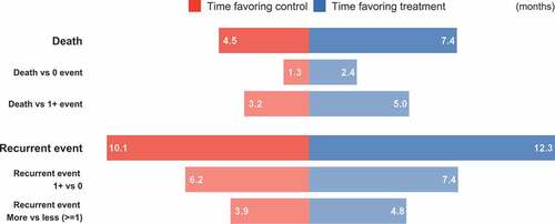Indeed, it was shown that the treatment on average gains the patient $\mu (\tau )=5.1$ months in a more favorable state in the first $\tau =4$ years post-randomization, including extra ${\mu }_{\mathrm{\infty }}(\tau )=2.9$ months survival time and ${\mu }_R(\tau )=2.2$ months living with fewer hospitalizations.

We look further into the two main components through the decompositions of (6). We find that the extra lifetime consists of 1.1 months hospitalization-free (standard error 0.52 and $p$-value 0.032) and 1.8 months having been hospitalized at least once (standard error 0.99 and $p$-value 0.076), a much more balanced composition than that in the colon cancer trial of Section 4.1. Likewise, the extra time spent living with fewer hospitalizations consists of 1.3 months hospitalization-free (standard error 1.2 and $p$-value 0.314) and 0.9 month having been hospitalized at least once (standard error 0.8 and $p$-value 0.215). The favorability plot in Figure 6 shows the structure of the effect sizes. The ${\chi }_2^2$ and ${\chi }_4^2$ joint tests yield $p$-values 0.039 and 0.173, respectively, both less significant than the ${\chi }_1^2$ overall test ($p$-value 0.018; see Mao (2023)) due to the largely homogeneous effects across components.

Figure 6. Favorability plot for the HF-ACTION trial at $\tau =4$ years.

5. Concluding remarks

Our dissection of the RMT-IF helps further reveal the makeup of the overall effect size. The resulting subcomponents, a product of state-to-state comparisons, provide detailed information about the changes in the average time spent in one state over another. Their estimation and inference are facilitated by the correspondence between the state probabilities and the survival functions of transition events, which allows the use of Kaplan--Meier curves to handle censored observations. These procedures will find use in the secondary analysis of composite endpoints, with the aim of understanding how the treatment affects different aspects of patient experience.

As a byproduct of component-wise inferences, their robust variance matrices have allowed us to construct joint tests, which empirically outperform the ${\chi }_1^2$ test on the overall RMT-IF when component-wise effects differ widely. To choose an optimal test in practice, the investigator should consider historical evidence on the heterogeneity of treatment effect as well as the current trial’s sample size (relative to which the test d.f. should be small). In any case, a decision must be made before looking at the data in order to maintain the correct type I error.

The restricting time also needs to be pre-specified. Ideally, the time window should be wide enough to be of clinical interest and to at least allow the treatment effect to come through. With $\tau =2.5$ years in the colon cancer trial of Section 4.1, for example, we could hardly see any improvement in patient survival (first row of Table 3), probably because the baseline mortality rate is still too low in such a short term. On the other hand, a restricting time beyond the last event in the data may cause numerical issues. Recently Tian et al. (2020) explored data-dependent choice of the time window for the RMST. A similar study could be done for the RMT-IF.

We have given a separate treatment to recurrent events and death as deserved by their special features. Since the transient (i.e., nonterminal) states, potentially many, are triggered by the same type of event, a meticulous state-to-state comparison feels unnecessary and cumbersome. The merge of intermediate states proposed in Section 2.4 reduces the number of subcomponents down to four, yet still allowing us to distinguish whether the patient has had any nonfatal events or not. Compared with the standard partition based on the specific number of event (Mao 2023), this new approach seems to strike a better balance between the level of detail and ease of interpretation.

Disclosure statement

No potential conflict of interest was reported by the authors.

Supplemental data

Supplemental data for this article can be accessed online at https://doi.org/10.1080/10543406.2023.2210658

Additional information

Funding

This research was supported by the National Institutes of Health grant R01HL149875.

Appendix

Rearranging the terms on the far right hand side of (4), we obtain that

(8) ${\mu }_{jk}(\tau )={\theta }_{j+1,k+1}(\tau )-{\theta }_{j+1,k}(\tau )-{\theta }_{j,k+1}(\tau )+{\theta }_{jk}(\tau ),$(8)

where

(9) ${\theta }_{jk}(\tau )={\int }_0^{\tau }\left\{S_j^{(1)}(t)S_k^{(0)}(t)-S_j^{(0)}(t)S_k^{(1)}(t)\right\}\mathrm{d}t.$(9)

Let ${\hat{\theta }}_{jk}(\tau )$ denote the estimator of ${\theta }_{j,k}(\tau )$ by substituting the Kaplan–Meier estimator ${\hat{S}}_l^{(a)}(t)$ for $S_l^{(a)}(t)$ $(l=j,k)$ in (9). If we can expand ${\hat{\theta }}_{jk}(\tau )$ asymptotically in the linear form

$n^{1/2}\{{\hat{\theta }}_{jk}(\tau )-{\theta }_{jk}(\tau )\}=q^{-1/2}{n}_1^{-1/2}\sum _{i=1}^{n_1}{\int }_0^{\tau }{\mathrm{\Psi }}_{ij}^{(1)}({\mathcal{O}}_i^{(1)})(t)\mathrm{d}t$

(10) $-(1-q{)}^{-1/2}{n}_0^{-1/2}\sum _{i=1}^{n_0}{\int }_0^{\tau }{\mathrm{\Psi }}_{ij}^{(0)}({\mathcal{O}}_i^{(0)})(t)\mathrm{d}t+o_p(1),$(10)

where $q={lim}_{n\to \mathrm{\infty }}{n}_1/n$ and the ${\mathrm{\Psi }}_{ij}^{(a)}({\mathcal{O}}^{(a)})(t)$ are some mean-zero influence functions (Tsiatis 2006), then by (8) we will have that

$n^{1/2}\{{\hat{\mu }}_{jk}(\tau )-{\mu }_{jk}(\tau )\}=q^{-1/2}{n}_1^{-1/2}\sum _{i=1}^{n_1}{\int }_0^{\tau }{\gamma }_{ij}^{(1)}({\mathcal{O}}_i^{(1)})(t)\mathrm{d}t$

(11) $-(1-q{)}^{-1/2}{n}_0^{-1/2}\sum _{i=1}^{n_0}{\int }_0^{\tau }{\gamma }_{ij}^{(0)}({\mathcal{O}}_i^{(0)})(t)\mathrm{d}t+o_p(1),$(11)

where ${\gamma }_{jk}^{(a)}({\mathcal{O}}^{(a)})(t)={\mathrm{\Psi }}_{j+1,k+1}^{(a)}({\mathcal{O}}^{(a)})(t)-{\mathrm{\Psi }}_{j+1,k}^{(a)}({\mathcal{O}}^{(a)})(t)-{\mathrm{\Psi }}_{j,k+1}^{(a)}({\mathcal{O}}^{(a)})(t)+{\mathrm{\Psi }}_{jk}^{(a)}({\mathcal{O}}^{(a)})(t)$. Let ${\hat{\gamma }}_{jk}^{(a)}(\cdot )(t)$ denote a nonparametric estimator of ${\gamma }_{jk}^{(a)}(\cdot )(t)$ (based on estimators for the ${\mathrm{\Psi }}_{jk}^{(a)}({\mathcal{O}}^{(a)})(t)$ below). Then, the asymptotic variance of ${\hat{\mu }}_{jk}(\tau )$ can be estimated by the empirical second moment

(12) $\widehat{\mathrm{v}\mathrm{a}\mathrm{r}}\{{\hat{\mu }}_{jk}(\tau )\}=n_1^{-2}\sum _{i=1}^{n_1}{\left\{{\int }_0^{\tau }{\hat{\gamma }}_{jk}^{(1)}({\mathcal{O}}_i^{(1)})(t)\mathrm{d}t\right\}}^2+n_0^{-2}\sum _{i=1}^{n_0}{\left\{{\int }_0^{\tau }{\hat{\gamma }}_{jk}^{(0)}({\mathcal{O}}_i^{(0)})(t)\mathrm{d}t\right\}}^2.$(12)

It now remains to derive and estimate ${\mathrm{\Psi }}_{ij}^{(a)}({\mathcal{O}}^{(a)})(t)$ in (10). By Corollary 3.2.1 of Fleming and Harrington (1991), the Kaplan–Meier estimator can be expanded by

$n_a^{1/2}\{{\hat{S}}_k^{(a)}(t)-S_k^{(a)}(t)\}=-n_a^{-1/2}{S}_k^{(a)}(t)\sum _{i=1}^{n_a}{\psi }_k^{(a)}({\mathcal{O}}_i^{(a)})(t)+o_p(1),$

where

${\psi }_k^{(a)}({\mathcal{O}}^{(a)})(t)={\int }_0^t{\pi }_k^{(a)}(s{)}^{-1}{M}_k^{(a)}(\mathrm{d}s;{\mathcal{O}}^{(a)}),$

${\pi }_k^{(a)}(s)=\mathrm{p}\mathrm{r}(X_k^{(a)}\ge s),$

$M_k^{(a)}\{s;{\mathcal{O}}^{(a)}\}=I\{X_k^{(a)}\le s,{\delta }_k^{(a)}=1\}-{\mathrm{\Lambda }}_k^{(a)}(X_k^{(a)}\wedge s),$

and ${\mathrm{\Lambda }}_k^{(a)}(\cdot )$ is the cumulative hazard function for $T_k^{(a)}$. We can estimate ${\psi }_k^{(a)}({\mathcal{O}}^{(a)})(t)$ by replacing ${\pi }_k^{(a)}(s)$ with its empirical analog and ${\mathrm{\Lambda }}_k^{(a)}(\cdot )$ with the standard Nelson–Aalen estimator. Denote the resulting estimator by ${\hat{\psi }}_k^{(a)}({\mathcal{O}}^{(a)})(t)$. Then, using the delta method on ${\hat{\theta }}_{jk}(\tau )$ as a functional of the ${\hat{S}}_j^{(a)}(t)$ and ${\hat{S}}_k^{(a)}(t)$ in (9), we find that

${\mathrm{\Psi }}_{ij}^{(a)}({\mathcal{O}}^{(a)})(t)=-S_k^{(1-a)}(t)S_j^{(a)}(t){\psi }_j^{(a)}({\mathcal{O}}_i^{(a)})(t)+S_k^{(a)}(t)S_j^{(1-a)}(t){\psi }_k^{(a)}({\mathcal{O}}_i^{(a)})(t),$

which can be estimated by substituting ${\hat{S}}_l^{(a)}(t)$ for $S_l^{(a)}(t)$ and ${\hat{\psi }}_l^{(a)}({\mathcal{O}}^{(a)})(t)$ for ${\psi }_l^{(a)}({\mathcal{O}}^{(a)})(t)$ $(l=j,k)$.

A.2 Construction of the joint tests

The robust variance matrix $\widehat{\sum \hspace{0.17em}}sub(\tau )$. can be constructed using the coordinate-wise influence functions in (11). Specifically, write

${\hat{\gamma }}^{(a)}(O^{(a)})(t)=\hspace{0.17em}\{{\hat{\gamma }}^{(a)}01(O^{(a)})(t),{\hat{\gamma }}^{02}(a)(O^{(a)})(t),{\hat{\gamma }}^{(a)}12(O^{(a)})(t),...,{\hat{\gamma }}^{(a)}K,K+1(O^{(a)})(t){\}}^{\mathrm{T}}$

Then by a similar construction to (12), we find that

${\widehat{\sum \hspace{0.17em}}}_{sub}(\tau )=n_1^{-2}\sum _{i=1}^{n_1}{\left\{{\int }_0^{\tau }{\hat{\gamma }}^{(1)}(O_i^{{ }^{(a)}})(t)dt\right\}}^{\oplus 2}+n_0^{-2}\sum _{i=1}^{n_0}{\left\{{\int }_0^{\tau }{\hat{\gamma }}^{(0)}(O_i^{{ }^{(a)}})(t)dt\right\}}^{\oplus 2}$

where $v^{\oplus }=v{v}^T$ for any vector $v$. The matrix $\widehat{\sum \hspace{0.17em}}main(\tau )$ can be derived similarly using the coordinate-wise influence functions of ${\hat{\mu }}_{main}(\tau )$ given in Proposition 1 of Mao (2023).

References

- Abdalla, S., M. E. Montez-Rath, P. S. Parfrey, and G. M. Chertow. 2016. The win ratio approach to analyzing composite outcomes: An application to the evolve trial. Contemporary Clinical Trials 48:119–124. doi:10.1016/j.cct.2016.04.001.
- Akacha, M., F. Bretz, D. Ohlssen, G. Rosenkranz, and H. Schmidli. 2017. Estimands and their role in clinical trials. Statistics in Biopharmaceutical Research 9 (3):268–271. doi:10.1080/19466315.2017.1302358.
- Anker, S. D., and J. V. McMurray. 2012. Time to move on from “time-to-first”: Should all events be included in the analysis of clinical trials. European Heart Journal 33 (22):2764–2765. doi:10.1093/eurheartj/ehs277.
- Armstrong, P. W., and C. M. Westerhout. 2017. Composite end points in clinical research: A time for reappraisal. Circulation 135 (23):2299–2307. doi:10.1161/CIRCULATIONAHA.117.026229.
- Buyse, M. 2010. Generalized pairwise comparisons of prioritized outcomes in the two-sample problem. Statistics in Medicine 29 (30):3245–3257. doi:10.1002/sim.3923.
- Crowther, M. J., and P. C. Lambert. 2017. Parametric multistate survival models: Flexible modelling allowing transition-specific distributions with application to estimating clinically useful measures of effect differences. Statistics in Medicine 36 (29):4719–4742. doi:10.1002/sim.7448.
- Cui, Y., G. Dong, P. F. Kuan, and B. Huang. 2022. Evidence synthesis analysis with prioritized benefit outcomes in oncology clinical trials. Journal of Biopharmaceutical Statistics 33 (3):272–288. doi:10.1080/10543406.2022.2141769.
- Dong, G., D. C. Hoaglin, B. Huang, Y. Cui, D. Wang, Y. Cheng, and M. Gamalo-Siebers. 2023. The stratified win statistics (win ratio, win odds, and net benefit). Pharmaceutical Statistics. doi:10.1002/pst.2293.
- Dong, G., B. Huang, Y. -W. Chang, Y. Seifu, J. Song, and D. C. Hoaglin. 2020. The win ratio: Impact of censoring and follow-up time and use with nonproportional hazards. Pharmaceutical Statistics 19 (3):168–177. doi:10.1002/pst.1977.
- Dong, G., B. Huang, J. Verbeeck, Y. Cui, J. Song, M. Gamalo-Siebers, D. Wang, D. C. Hoaglin, Y. Seifu, T. Mütze, et al. (2022). Win statistics (win ratio, win odds, and net benefit) can complement one another to show the strength of the treatment effect on time-to-event outcomes. Pharmaceutical Statistics 10.1002/pst.2251.
- Dong, G., J. Qiu, D. Wang, and M. Vandemeulebroecke. 2018. The stratified win ratio. Journal of Biopharmaceutical Statistics 28 (4):778–796. doi:10.1080/10543406.2017.1397007.
- Finkelstein, D. M., and D. A. Schoenfeld. 1999. Combining mortality and longitudinal measures in clinical trials. Statistics in Medicine 18 (11):1341–1354. doi:10.1002/(SICI)1097-0258(19990615)18:11<1341:AID-SIM129>3.0.CO;2-7.
- Fleming, T. R., and D. P. Harrington. 1991. Counting Processes and Survival Analysis. Hoboken, NJ: John Wiley & Sons.
- Freemantle, N., M. Calvert, J. Wood, J. Eastaugh, and C. Griffin. 2003. Composite outcomes in randomized trials: Greater precision but with greater uncertainty. Journal of the American Medical Association 289 (19):2554–2559. doi:10.1001/jama.289.19.2554.
- Kandzari, D. E., G. L. Hickey, S. J. Pocock, M. A. Weber, M. Boehm, S. A. Cohen, M. Fahy, G. Lamberti, and F. Mahfoud. 2021. Prioritised endpoints for device-based hypertension trials: The win ratio methodology. EuroIntervention: Journal of EuroPcr in Collaboration with the Working Group on Interventional Cardiology of the European Society of Cardiology 16 (18):e1496–1502. doi:10.4244/EIJ-D-20-01090.
- Mao, L. 2023. On restricted mean time in favor of treatment. Biometrics 79 (1):61–72. doi:10.1111/biom.13570.
- Mao, L., and K. Kim. 2021. Statistical models for composite endpoints of death and non-fatal events: A review. Statistics in Biopharmaceutical Research 13 (3):260–269. doi:10.1080/19466315.2021.1927824.
- Mao, L., K. Kim, and Y. Li. 2022. On recurrent-event win ratio. Statistical Methods in Medical Research 31 (6):1120–1134. doi:10.1177/09622802221084134.
- Maurer, M. S., J. H. Schwartz, B. Gundapaneni, P. M. Elliott, G. Merlini, M. Waddington-Cruz, A. V. Kristen, M. Grogan, R. Witteles, T. Damy, et al. 2018. Tafamidis treatment for patients with transthyretin amyloid cardiomyopathy. The New England Journal of Medicine. 379(11):1007–1016. doi:10.1056/NEJMoa1805689.
- McCaw, Z. R., G. Yin, and L. -J. Wei. 2019. Using the restricted mean survival time difference as an alternative to the hazard ratio for analyzing clinical cardiovascular studies. Circulation 140 (17):1366–1368. doi:10.1161/CIRCULATIONAHA.119.040680.
- Moertel, C. G., T. R. Fleming, J. S. Macdonald, D. G. Haller, J. A. Laurie, P. J. Goodman, J. S. Ungerleider, W. A. Emerson, D. C. Tormey, J. H. Glick, et al. 1990. Levamisole and fluorouracil for adjuvant therapy of resected colon carcinoma. The New England Journal of Medicine. 322(6):352–358. doi:10.1056/NEJM199002083220602.
- Oakes, D. 1989. Bivariate survival models induced by frailties. Journal of the American Statistical Association 84 (406):487–493. doi:10.1080/01621459.1989.10478795.
- Oakes, D. 2016. On the win-ratio statistic in clinical trials with multiple types of event. Biometrika 103 (3):742–745. doi:10.1093/biomet/asw026.
- O’Connor, C. M., D. J. Whellan, K. L. Lee, S. J. Keteyian, L. S. Cooper, S. J. Ellis, E. S. Leifer, W. E. Kraus, D. W. Kitzman, J. A. Blumenthal, et al. 2009. Efficacy and safety of exercise training in patients with chronic heart failure: Hf-action randomized controlled trial. Journal of the American Medical Association. 301(14):1439–1450. doi:10.1001/jama.2009.454.
- Pocock, S., C. Ariti, T. Collier, and D. Wang. 2012. The win ratio: A new approach to the analysis of composite endpoints in clinical trials based on clinical priorities. European Heart Journal 33 (2):176–182. doi:10.1093/eurheartj/ehr352.
- Redfors, B., J. Gregson, A. Crowley, T. McAndrew, O. Ben-Yehuda, G. W. Stone, and S. J. Pocock. 2020. The win ratio approach for composite endpoints: Practical guidance based on previous experience. European Heart Journal 41 (46):4391–4399. doi:10.1093/eurheartj/ehaa665.
- Royston, P., and M. K. Parmar. 2011. The use of restricted mean survival time to estimate the treatment effect in randomized clinical trials when the proportional hazards assumption is in doubt. Statistics in Medicine 30 (19):2409–2421. doi:10.1002/sim.4274.
- Seifu, Y., S. Mt-Isa, K. Duke, M. Gamalo-Siebers, W. Wang, G. Dong, and J. Kolassa. 2022. Design of paediatric trials with benefit-risk endpoints using a composite score of adverse events of interest (aei) and win-statistics. Journal of Biopharmaceutical Statistics 1–12. doi:10.1080/10543406.2022.2153202.
- Tian, L., H. Fu, S. J. Ruberg, H. Uno, and L. -J. Wei. 2018. Efficiency of two sample tests via the restricted mean survival time for analyzing event time observations. Biometrics 74 (2):694–702. doi:10.1111/biom.12770.
- Tian, L., H. Jin, H. Uno, Y. Lu, B. Huang, K. M. Anderson, and L. Wei. 2020. On the empirical choice of the time window for restricted mean survival time. Biometrics 76 (4):1157–1166. doi:10.1111/biom.13237.
- Tsiatis, A. 2006. Semiparametric Theory and Missing Data. New York: Springer.
- Uno, H., B. Claggett, L. Tian, E. Inoue, P. Gallo, T. Miyata, D. Schrag, M. Takeuchi, Y. Uyama, L. Zhao, et al. 2014. Moving beyond the hazard ratio in quantifying the between-group difference in survival analysis. Journal of Clinical Oncology. 32(22):2380. doi:10.1200/JCO.2014.55.2208.
- Vardeny, O., K. Kim, J. A. Udell, J. Joseph, A. S. Desai, M. E. Farkouh, S. M. Hegde, A. F. Hernandez, A. McGeer, H. K. Talbot, et al. 2021. Effect of high-dose trivalent vs standard-dose quadrivalent influenza vaccine on mortality or cardiopulmonary hospitalization in patients with high-risk cardiovascular disease: A randomized clinical trial. JAMA. 325(1):39–49. doi:10.1001/jama.2020.23649.