Estimating treatment effect in randomized trial after control to treatment crossover using external controls

ABSTRACT

In clinical trials, it is common to design a study that permits the administration of an experimental treatment to participants in the placebo or standard of care group post primary endpoint. This is often seen in the open-label extension phase of a phase III, pivotal study of the new medicine, where the focus is on assessing long-term safety and efficacy. With the availability of external controls, proper estimation and inference of long-term treatment effect during the open-label extension phase in the absence of placebo-controlled patients are now feasible. Within the framework of causal inference, we propose several difference-in-differences (DID) type methods and a synthetic control method (SCM) for the combination of randomized controlled trials and external controls. Our realistic simulation studies demonstrate the desirable performance of the proposed estimators in a variety of practical scenarios. In particular, DID methods outperform SCM and are the recommended methods of choice. An empirical application of the methods is demonstrated through a phase III clinical trial in rare disease.

KEYWORDS:

• Open-label extension
• causal inference
• treatment crossover
• long-term treatment effect
• external controls
• real-world data
• difference-in-differences
• synthetic control

1. Introduction

Randomized controlled trials (RCTs) are considered the gold standard for estimating the treatment effect of a therapeutic product on an outcome of interest in a particular disease. Due to ethical consideration, it is not feasible to maintain a blinded, placebo-controlled treatment assignment in a clinical trial for an extended period. But for medications treating chronic or slow degenerative diseases, long-term efficacy assessment is crucial for patients and health practitioners. Open-label extension phase of a phase III study, providing a potential opportunity for long-term effectiveness evaluation, is widely used (Day and Williams 2007). It extends a phase III, randomized placebo-controlled, pivotal study of the new medicine, during which the placebo group (hence all patients) will receive the trial medicine. Allowing the placebo or standard of care group to crossover to the experimental treatment after some time is a way to make such studies more attractive for patients.

Lacking a control group during the open-label extension phase poses a challenge to assess the treatment effect on the efficacy outcomes. A promising approach is to harness the RCT data with the so-called “external controls” (Wang et al. 2022; Yap et al. 2021). “External controls” referring to a comparison group of people external to the trial of interest who had not received the experimental treatment, is gaining traction in regulatory agencies (FDA 2023) and industry (Burger et al. 2021). The use of external controls aims to harness the RCTs by either fully or partially substituting the trial control arms. Although various sources of data can serve as external controls, they are primarily derived from patient-level data from other clinical trials or from real-world data (RWD) sources. The use of a control group from other trials is feasible if the eligible population and endpoints align closely with the current study, as demonstrated in our motivating example introduced later (McIver et al. 2023).

The use of external controls provides valuable information about disease progression in the absence of the experimental treatment. The fused data of RCT with external controls contains both treated and untreated patients, creating the possibility for estimation of treatment effects during periods when the internal control arm in the RCT has switched to the treatment. However, this combination lacks the fundamental ignorability property resulting from randomization, as patients are not randomly assigned to either the trial or the external control group. Directly pooling external controls to estimate treatment effects on the trial population can lead to biased results, irrespective of sample size. To address this challenge, causal inference methods provide a principled framework to incorporate real-world data in clinical trials, as advocated by recent research (Ho et al. 2021).

This work is motivated by a recent study of the medicine risdiplam to treat spinal muscular atrophy (SMA). The SUNFISH Trial (NCT02908685) is a phase 3, randomized, double-blind, placebo-controlled study of the efficacy and safety of the medicine risdiplam treatment among patients aged 2–25 years with confirmed 5q autosomal recessive type 2 or type 3 SMA. Patients were stratified by age and randomly assigned (2:1) to receive either daily oral risdiplam or daily oral placebo. The phase 3 study consisted of two periods. The first 12-month was a randomized placebo-controlled design with two arms. Patients were scheduled for regular followup visits to have their Motor Function Measure (MFM) measured along with other clinically relevant indicators. The primary endpoint was the change in the MFM from baseline to the end of month 12. Though the primary endpoint was captured and analyzed at the end of the first 12-month, the trial continued for a second 12-month open-label extension phase during which all patients in the control arm were switched to the risdiplam arm. The results in the primary endpoint have shown a significant improvement in motor function compared with placebo. More information about the trial can be found in Mercuri et al. (2022). The second 12-month period was designed to investigate the efficacy of risdiplam treatment beyond 12 months, as stated in the exploratory objective of the trial.

The objective of the 12-month randomized comparison was to adequately establish the efficacy of the new therapy. But further follow up beyond 12 months is needed to understand its long-term benefit, which raises methodological challenges that are of particular interest to us. For a disease such as SMA, which has limited treatment options, having a control group for long-term assessment has both practical and ethical implications. First, patients will progress over time and will never regain function lost during progression. It is therefore unethical to maintain placebo control for too long. Secondly, there can be feasibility issues when trying to maintain randomization for too long. Trial results may become non-interpretable due to excessive rates of protocol violations and drop outs. Therefore, trials with such a period without placebo-controlled arm to assess long-term effect are common and practical for diseases with limited options or progressive diseases in general, and the SUNFISH trial serves as a representative example of these challenges.

However, information about the disease progression without treatment often exists in trials designed for other treatment comparisons or RWD. For instance, the olesoxime trial (NCT01302600) (Berry et al. 2010) is a randomized, double-blind, placebo-controlled, phase 2 study for the same disease population as SUNFISH. The olesoxime trial shares the same set of measurements and follow-up visits as the SUNFISH study, but with a control arm that spans over 2 years, which can serve as external controls to augment the SUNFISH study (McIver et al. 2023). It is also possible to find external controls from RWD, e.g. registries, which go beyond one or two years.

The situation we consider differs from the application of external control data in other instances. First, there is no alternative anymore as we start with a randomized trial but cannot maintain the randomization for too long. Therefore the randomized assignment is no longer present for long-term follow up evaluations and we can leverage the use of external controls for statistical estimation and inference. Secondly, we have a randomized control group followed up for short term, which could be used to adjust the external controls and check assumptions made.

Our main contributions in this paper are to adapt the ideas of difference-in-differences methods (Abadie 2005; Sant’anna and Zhao 2020), and synthetic control methods (Abadie et al. 2010) to the problem of augmenting RCT with external controls in the study design described above.

The remainder of this paper is organized as follows. In Section 2 we introduce the notation, define the estimand, and discuss the causal assumptions that are realistic for the setting. In Section 3 we describe our two proposed approaches: difference-in-differences methods and synthetic control methods, and briefly introduce the reference-based multiple imputation as an alternative method for comparison. We then present simulation studies to demonstrate the performance of the proposed methods in settings likely to occur in real trials, in Section 4 In Section 5, we demonstrate the applicability of proposed methods using our motivating study. Finally, Section 6 discusses practical takeaways for this research.

2. Notation, estimand, and causal assumptions

2.1. Notations

We have two datasets at hand: (1) an RCT with open-label extension phase, denoted by $\mathcal{R}$ (for two-phase RCT), and (2) an external control sample, denoted by $\mathcal{E}$ (for external control). We will use indices $\mathcal{R}$ and $\mathcal{E}$ to denote quantities taken with respect to different study populations. We use subscript $\mathit{i}$ to denote the $\mathit{i}$th patient in the pooled dataset. Let $S_i$ denote trial participation status, with $S_i=1$ for patients in the two-phase RCT and $S_i=0$ for external control patients.

Let’s denote a p-dimensional vector of baseline covariates that could influence participation in either the two-phase RCT or the external study and are simultaneously risk factors for the outcome as ${\mathbf{W}}_i=({\mathbf{X}}_i,{\mathbf{U}}_i)$, where ${\mathbf{X}}_i$ is $p_X$-dimensional measured covariates and ${\mathbf{U}}_i$ is $p_U$-dimensional unmeasured covariates. This implies that these variables act as confounders between the outcomes and the study participation.

Consider the sequence of binary treatment assignments ${\mathbf{A}}_i=(A_{\mathit{i}1},A_{\mathit{i}2})$ structured to accommodate the two-phase RCT as follows: $(1,1)$ corresponds to patients from the RCT who were assigned to the treatment group in the first randomized controlled phase and continued to be treated in the second open-label extension phase; $(0,1)$corresponds to patients from the RCT who were assigned to the control group during the first randomized controlled phase, but were later switched to receive treatment in the second open-label extension phase; and $(0,0)$ corresponds to patients from the external control pool since they were never treated. In this context, only $A_{\mathit{i}1}$ is subject to randomization with a probability of ${\pi }_A$ for RCT patients. Once $A_{\mathit{i}1}$ is established, $A_{\mathit{i}2}$ is then determined as per the design of the study. Therefore, the treatment assignment ${\mathbf{A}}_i$ is influenced solely by $S_i$, and any potential confounding bias arises from potentially unbalanced selection of study participants $S_i$, not from a treatment assignment.

We acknowledge that study participation $S_i$ could directly influence the outcomes, separate from the effect of the treatment. This could be explained by the fact that patients participating in the RCT may experience closer monitoring, superior care, or other distinctive conditions that could eventually impact the outcomes.

Lastly, we have longitudinal outcomes ${\mathbf{Y}}_i=\left(Y_{\mathit{i}1},\dots ,Y_{i{T}_1},\dots ,Y_{i{T}_2}\right)$ which are repeatedly measured at $T_2$ discrete time points spread over two phases: the first randomized, placebo-controlled period ${\mathcal{T}}_1=(0,T_1]$, and the second open-label extension period ${\mathcal{T}}_2=(T_1,T_2]$. In the context of the SUNFISH study, there are 2 observations in each of the two phases with approximately six months separating each measurement, which corresponds to $T_1=2$ and $T_2=4$.

Our observed data are $\mathit{n}$ independent and identically distributed observations $O_i=\left({\mathbf{X}}_i,S_i,{\mathbf{A}}_i,{\mathbf{Y}}_i\right)$ for $\mathit{i}\in \mathcal{R}\cup \mathcal{E}$, with $\mathit{n}$ RCT patients and $\mathit{m}$ external control patients, where $\mathcal{R}$ ($|\mathcal{R}|=\mathit{n}$) and $\mathcal{E}$ ($|\mathcal{E}|=\mathit{m}$) are sets of indices for the two-phases RCT subjects and external control subjects, respectively.

Working under the potential outcome framework (Imbens and Rubin 2015), let ${\mathbf{Y}}_i^{(s,\mathbf{a})}=\left(Y_{i1}^{(s,\mathbf{a})},\dots ,Y_{i{T}_1}^{(\mathit{s},\mathbf{a})},\dots ,Y_{i{T}_2}^{(\mathit{s},\mathbf{a})}\right)$ be the time-indexed potential outcomes had the patient $\mathit{i}$ participated in the study $\mathit{s}\in \{0,1\}$and gone through the sequence of treatment $\mathbf{a}\in \{(1,1),(0,1),(0,0)\}$. Here, the potential outcomes depend on both the study participation and treatment sequence.

2.2. Estimand

The objective is to estimate the average treatment effect (ATE) for the RCT population during the open-label extension phase, which quantify the long-term treatment effect evolution:

(1) ${\tau }_t={\mathbb{E}}_{\mathcal{R}}\left[Y_t^{(1,(1,1))}-Y_t^{(1,(0,0))}\right],\mathrm{for}\mathit{t}\in {\mathcal{T}}_2.$(1)

where the expectation is with respect to the RCT population.

2.3. Causal assumptions

We first state two assumptions that are standard and generally hold.

Assumption 1

(Stable unit treatment value (SUTVA)). Consistency and no interference hold, i.e. the observed outcome equals to the potential outcome under the actual study and treatment sequence received: ${\mathbf{Y}}_i={\mathbf{Y}}_i^{(S_i,{\mathbf{A}}_i)}$, for $\mathit{i}\in \mathcal{R}\cup \mathcal{E},S_i\in \{0,1\},{\mathbf{A}}_i\in \left\{(0,0),(0,1),(1,1)\right\}$.

Assumption 2

(Internal validity of the trial). (a) Initial treatment randomization holds for all RCT patients, that is: ${\mathbf{Y}}_i^{(1,\mathbf{a})}\mathrm{\perp }{\mathbf{A}}_{\mathit{i}1}|S_i=1$, for ${\mathbf{A}}_{\mathit{i}1}\in \left\{0,1\right\},\mathbf{a}\in \left\{(1,1),(0,1)\right\}$;

(b) Positivity of trial treatment assignment holds, that is: $0<{\pi }_A<1$.

Figure 1 represents a Directed Acyclic Graph (DAG) (Pearl 2009) encoding our knowledge about the mechanism between covariates, interventions and outcomes, for the RCT and external controls pooled data.

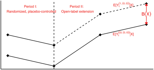
Figure 1. Graphical model representing the pooled dataset. The node ${\mathbf{Y}}_I=(Y_1\dots Y_{T_1})$ represents the repeated measures during the randomized controlled phase, and ${\mathbf{Y}}_{\mathit{II}}=(Y_{T_1+1}\dots Y_{T_1+T_2})$ represents the open-label extension phase.

The most commonly invoked causal assumption is the conditional ignorability of trial participation in the literature of combining experimental and observational data, analogous to the unconfoundedness assumption for observational studies (Rubin 1977) (synonymous to the selection on observables or exogeneity assumption). There has been a wealth of research built upon this type of assumption, for different purposes and under different terms: generalizability (Buchanan et al. 2018; Cole and Stuart 2010; Dahabreh and Hernán 2019), representativeness (Campbell 1957), external validity (Stuart et al. 2018), transportability (Pearl and Bareinboim 2011; Westreich et al. 2017), and data fusion (Bareinboim and Pearl 2016). However, it might be too strong in practice. Two features in Figure 1 invalidate this assumption, as described below.

First, there could exist unmeasured baseline confounders $\mathbf{U}$ between trial participation and the outcomes. In practical term, this means both the trial and the external study must capture all risk factors of the outcomes that also influence study participation. This might include demographic, socioeconomic, and disease features. For example, rare disease patients may differ in terms of access to high-quality care, financial resources, or general living conditions, that might make some patients less likely to participate in the RCT, and coincidentally, these same conditions could exacerbate the progression of the disease. Therefore, the population participating in the trial could be self-selected in a way that differs from the external control population in manners that investigators are unaware of.

Second, the trial participation may have a direct effect on the outcomes. This is illustrated in Figure 1 by the path $\mathit{S}\to ({\mathbf{Y}}_I,{\mathbf{Y}}_{\mathit{II}})$. This might include study bias and placebo effect. For example, patients in the clinical trial might be monitored more closely, receive better care, or simply being measured differently.

The above reasons, illustrated by the unblocked back-door path $\mathit{S}\leftarrow \mathit{U}\to {\mathbf{Y}}_{\mathit{II}}$ and a front-door path $\mathit{S}\to {\mathbf{Y}}_{\mathit{II}}$, imply that trial patients and external control patients are not exchangeable, given the measured characteristics. Therefore, we do not reply on the ignorability assumption. Different methods for estimating the treatment effect during the open-label extension phase are discussed in subsequent sections which depend on various forms of more relaxed assumptions to be specified in Section 2, allowing the existence of unmeasured confounders and direct effect of trial participation.

3. Methods

Let $n_1\times T_1$ matrix ${\mathit{Y}}_{\mathrm{t},I}^{\mathrm{o}\mathrm{b}\mathrm{s}}$ and $n_1\times (T_2-T_1)$ matrix ${\mathit{Y}}_{\mathrm{t},II}^{\mathrm{o}\mathrm{b}\mathrm{s}}$ denote the stacked observed outcome matrix for two-phase RCT patients receiving treatment sequence $(1,1)$ in the randomized controlled phase and open-label extension phase, respectively. Similarly, define $n_0\times T_1$ matrix ${\mathit{Y}}_{\mathrm{c},I}^{\mathrm{o}\mathrm{b}\mathrm{s}}$ and $n_0\times (T_2-T_1)$ matrix ${\mathit{Y}}_{\mathrm{c},II}^{\mathrm{o}\mathrm{b}\mathrm{s}}$ for RCT patients receiving treatment sequence $(0,1)$, and $\mathit{m}\times T_1$ matrix ${\mathit{Y}}_{\mathrm{e},I}^{\mathrm{o}\mathrm{b}\mathrm{s}}$ and $\mathit{m}\times (T_2-T_1)$ matrix ${\mathit{Y}}_{\mathrm{e},II}^{\mathrm{o}\mathrm{b}\mathrm{s}}$ for external control patients. In addition, let ${\mathit{Y}}_I^{(s,\mathbf{a})}$ and ${\mathit{Y}}_{II}^{(s,\mathbf{a})}$ be the stacked potential outcome matrices if participated in study $\mathit{s}\in \{0,1\}$ and received treatment $\mathbf{a}\in \{(0,0),(0,1),(1,1)\}$. By Assumption 1, a subset of potential outcomes are observed, and the relation between observed outcomes and potential outcomes is

$\left(\begin{array}{cc}{\mathit{Y}}_{\mathrm{t},I}^{\mathrm{o}\mathrm{b}\mathrm{s}}& {\mathit{Y}}_{\mathrm{t},II}^{\mathrm{o}\mathrm{b}\mathrm{s}}\\ {\mathit{Y}}_{\mathrm{c},I}^{\mathrm{o}\mathrm{b}\mathrm{s}}& {\mathit{Y}}_{\mathrm{c},II}^{\mathrm{o}\mathrm{b}\mathrm{s}}\\ {\mathit{Y}}_{\mathrm{e},I}^{\mathrm{o}\mathrm{b}\mathrm{s}}& {\mathit{Y}}_{\mathrm{e},II}^{\mathrm{o}\mathrm{b}\mathrm{s}}\end{array}\right)=\left(\begin{array}{cc}{\mathit{Y}}_I^{(1,(1))}& {\mathit{Y}}_{II}^{(1,(1,1))}\\ {\mathit{Y}}_I^{(1,(0))}& {\mathit{Y}}_{II}^{(1,(0,1))}\\ {\mathit{Y}}_I^{(0,(0))}& {\mathit{Y}}_{II}^{(0,(0,0))}\end{array}\right)$

The causal estimand of interest can be estimated by the pair of matrices ${\mathit{Y}}_{II}^{(1,(1,1))}$ (always-treated RCT patient outcomes in open-label extension phase) and ${\mathit{Y}}_{II}^{(1,(0,0))}$ (never-treated RCT patient outcomes in open-label extension phase). The former is observed in the group of RCT patients who received treatment sequence $(1,1)$, but the latter is not due to switching initial control arm to be treated in the open-label extension phase. So, the problem can be viewed as a missing data problem where the never-treated outcomes for RCT patients need to be estimated or imputed.

Notice that we have three different sets of outcomes without treatment contamination, ${\mathit{Y}}_I^{(1,(0))}$ (RCT initial control during first phase), ${\mathit{Y}}_I^{(0,(0))}$ (external control during first phase), and ${\mathit{Y}}_{II}^{(0,(0,0))}$ (external control during second phase). Given that the difficulty is due to the unobservable, counterfactual, never-treated outcomes for trial subjects ${\mathit{Y}}_{II}^{(1,(0,0))}$, the question is how to model the relation between the three observable sets and the unobservable in order to impute the latter.

$\left(\begin{array}{cc}{\mathit{Y}}_I^{(1,(0))}& {\mathit{Y}}_{II}^{(1,(0,0))}=?\\ {\mathit{Y}}_I^{(0,(0))}& {\mathit{Y}}_{II}^{(0,(0,0))}\end{array}\right)$

This perspective opens the connection with an extensive body of literature on determining the impact of non-randomized interventions in longitudinal data settings, a common situation in social sciences, and enables us to draw upon novel statistical methods.

3.1. Approach 1: difference-in-differences type methods

To estimate the counterfactual never-treated outcomes for trial patients during the open-label extension phase, using the observed outcomes of the external control patients during the same period can result in (conditional) bias $\mathit{B}(\mathbf{X},\mathit{t}):=\mathbb{E}\left[Y_t^{(1,(0,0))}-Y_t^{(0,(0,0))}|\mathbf{X}\right]$. In general, the bias depends on both the measured baseline confounders $\mathbf{X}$ and time $\mathit{t}$, and unfortunately, is never known a priori. It only disappears under the more stringent ignorability assumption which we do not assume.

The open-label extension phase following a randomized controlled trial provides a negative control (NC) situation to approximate this bias term. The essential purpose of a NC is to reproduce a condition that cannot involve the hypothesized causal mechanism, but is very likely to involve the same sources of bias, and have been used to detect residual confounding in epidemiology (Lipsitch et al. 2010). In our setting, the outcomes in the randomized controlled phase, ${\mathit{Y}}_{c,I}^{\mathrm{o}\mathrm{b}\mathrm{s}}={\mathit{Y}}_I^{(1,(0))}$ and ${\mathit{Y}}_{e,I}^{\mathrm{o}\mathrm{b}\mathrm{s}}={\mathit{Y}}_I^{(0,(0))}$ can be used as NCs for estimating ${\mathit{Y}}_{II}^{(1,(0,0))}$ using ${\mathit{Y}}_{e,II}^{\mathrm{o}\mathrm{b}\mathrm{s}}={\mathit{Y}}_{II}^{(0,(0,0))}$, as the relation between trial participation and the two sets of never-treated outcomes, one in the first randomized controlled phase and one in the open-label extension phase, should share same source of bias, such as the unmeasured confounding bias and direct effect of trial participation. The idea of using first phase outcomes as NCs also coincides with idea of the difference-in-differences (DID) methods (Abadie 2005; Heckman et al. 1998; Sant’anna and Zhao 2020).

We formalize the assumption that enables the identification of the bias term, and hence the estimand.

Assumption 3

(Conditional Parallel Trends). The conditional bias only depends on the measured baseline covariates but not time $\mathit{t}$, in other words, the average potential outcome trajectories under no treatment for the trial and external control patients would have followed parallel path over time, given measured baseline covaraites, as illustrated in Figure 2.

$\mathit{B}(\mathbf{X},\mathit{t}):=\mathbb{E}\left[Y_t^{(1,(0,0))}-Y_t^{(0,(0,0))}|\mathbf{X}\right]=\mathit{B}(\mathbf{X})\mathit{for}\mathit{all}\mathit{t}\in {\mathcal{T}}_1\cup {\mathcal{T}}_2\mathit{and}\mathbf{X}$

See Remark 6 in Appendix A for a discussion of the verifiability.

Figure 2. Illustration of the conditional parallel trends assumption.

Remark 1. Assumption 3 is satisfied if never-treated outcomes of the trial and external control patients follows the linear factor model

(2) $Y_t^{(s,(0,0))}={\delta }_t+{\theta }_t^T\mathbf{X}+{\lambda }^T\mathbf{U}+{\mathrm{\Delta }}_s\mathit{S}+{\epsilon }_t$(2)

for $\mathit{t}\in {\mathcal{T}}_1\cup {\mathcal{T}}_2$, where ${\delta }_t$ is an unknown time-varying common factor shared by all patients, ${\theta }_t$ and $\mathit{\lambda }$ are vectors of coefficients associated with measured and unmeasured baseline confounders, respectively, and ${\mathrm{\Delta }}_s$ is the direct effect of trial participation. Note that both $\mathit{\lambda }$ and $\mathrm{\Delta }$ are time-constant, indicating that the unmeasured confounding bias and the direct effect of trial participation only exert a consistent, unchanging impact on outcomes over time.

Under causal asssumptions 1, 2 and 3, we present three identification formulae for the estimand in Eq. 1: DID-EC-OR (outcome regression) approach, DID-EC-IPW (inverse probability weighting) approach, and DID-EC-AIPW (augmented inverse probability weighting) approach, inspired by (Abadie 2005; Heckman et al. 1998; Sant’anna and Zhao 2020).

For $\mathit{t}\in {\mathcal{T}}_2,$

(3) $\begin{array}{rl}{\tau }_t^{\mathrm{D}\mathrm{I}\mathrm{D}-\mathrm{E}\mathrm{C}-\mathrm{O}\mathrm{R}}=& {\mathbb{E}}_{\mathcal{R}}\left[\underset{{\mathrm{\Delta }}_{\mathit{trial}}}{\underbrace{\left(\mathit{\mu }(\mathbf{X},S=1,\mathbf{A}=(1,1),t)-\bar{\mu }(\mathbf{X},\mathit{S}=1,A_1=0,{\mathcal{T}}_1)\right)}}\right.\\ & \left.-\underset{{\mathrm{\Delta }}_{\mathit{EC}}}{\underbrace{\left(\mathit{\mu }(\mathbf{X},S=0,\mathbf{A}=(0,0),t)-\bar{\mu }(\mathbf{X},\mathit{S}=0,A_1=0,{\mathcal{T}}_1)\right)}}\right]\\ & \end{array}$(3)

(4) $\begin{array}{rl}{\tau }_t^{\mathrm{D}\mathrm{I}\mathrm{D}-\mathrm{E}\mathrm{C}-\mathrm{I}\mathrm{P}\mathrm{W}}=& \underset{{\mathrm{\Delta }}_{\mathit{trial}}}{\underbrace{{\mathbb{E}}_{\mathcal{R}}\left[\frac{A_1{W}_{11}}{{\mathbb{E}}_{\mathcal{R}}\left[A_1{W}_{11}\right]}{Y}_t-\frac{(1-A_1)W_{10}}{{\mathbb{E}}_{\mathcal{R}}\left[(1-A_1)W_{10}\right]}\bar{Y}({\mathcal{T}}_1)\right]}}\\ & -\underset{{\mathrm{\Delta }}_{\mathit{EC}}}{\underbrace{{\mathbb{E}}_{\mathcal{E}}\left[\frac{W_0(\mathbf{X})}{{\mathbb{E}}_{\mathcal{E}}\left[W_0(\mathbf{X})\right]}\left(Y_t-\bar{Y}({\mathcal{T}}_1)\right)\right]}}\end{array}$(4)

(5) $\begin{array}{rl}{\tau }_t^{\mathrm{D}\mathrm{I}\mathrm{D}-\mathrm{E}\mathrm{C}-\mathrm{A}\mathrm{I}\mathrm{P}\mathrm{W}}=& \underset{{\mathrm{\Delta }}_{\mathit{trial}}}{\underbrace{{\mathbb{E}}_{\mathcal{R}}\left[\frac{A_1{W}_{11}}{{\mathbb{E}}_{\mathcal{R}}\left[A_1{W}_{11}\right]}{\tilde{Y}}_{\mathit{t}}-\frac{(1-A_1)W_{10}}{{\mathbb{E}}_{\mathcal{R}}\left[(1-A_1)W_{10}\right]}\bar{\tilde{Y}}({\mathcal{T}}_1)\right]}}\\ & -\underset{{\mathrm{\Delta }}_{\mathit{EC}}}{\underbrace{{\mathbb{E}}_{\mathcal{E}}\left[\frac{W_0(\mathbf{X})}{{\mathbb{E}}_{\mathcal{E}}\left[W_0(\mathbf{X})\right]}\left({\tilde{Y}}_{\mathit{t}}-\bar{\tilde{Y}}({\mathcal{T}}_1)\right)\right]}}\end{array}$(5)

where in Eq.3, $\mathit{\mu }(\mathbf{X},\mathit{S},\mathbf{A},\mathit{t})$ represents the true conditional expected outcome given the covariates, study participation, treatment assignment, and time, and accordingly, $\bar{\mu }(\mathbf{X},\mathit{S},\mathbf{A},{\mathcal{T}}_1)=\frac{1}{T_1}{\sum }_{\mathit{t}\in {\mathcal{T}}_1}\mathit{\mu }(\mathbf{X},\mathit{S},\mathbf{A},\mathit{t})$ is the true conditional expected outcomes averaged over the randomized controlled phase. In Eq. 4 and 5 the trial treated, trial control, and external control patients receive weights $W_{11}=1/{\pi }_A$, $W_{10}=1/(1-{\pi }_A)$, and $W_0(\mathbf{X})=\frac{{\mathit{p}}_{\mathcal{R}}(\mathbf{X})}{p_{\mathcal{E}}(\mathbf{X})}$, respectively. $W_0(\mathbf{X})$ can be thought of as a special case of the balancing weights in (Li et al. 2018) to match the measured covariate distribution of the external controls to that of the trial patients. $\bar{Y}({\mathcal{T}}_1)=\frac{1}{T_1}{\sum }_{\mathit{t}\in {\mathcal{T}}_1}{Y}_t$ is average of outcomes in the first randomized controlled phase. ${\tilde{Y}}_{\mathit{t}}=Y_t-\mathit{\mu }(\mathbf{X},\mathit{S}=0,\mathbf{A}=(0,0),\mathit{t})$ is the residual after projection using the outcome regression model for the external controls, and $\bar{\tilde{Y}}({\mathcal{T}}_1)=\frac{1}{T_1}{\sum }_{\mathit{t}\in {\mathcal{T}}_1}{\tilde{Y}}_{\mathit{t}}$ is the average of such residuals in the first phase.

Remark 2. In addition to the rationale for using the randomized controlled phase outcomes as negative controls based on Assumption 3, the three variants can be interpreted as the difference between two differences, hence the name difference-in-differences (DID): ${\mathrm{\Delta }}_{\mathit{trial}}$ represents the expected difference between always-treated outcomes during the open-label extension phase and untreated outcomes during the randomized controlled phase, for trial patients, while ${\mathrm{\Delta }}_{\mathit{EC}}$ represents the expected difference between never-treated outcomes during the open-label extension phase and untreated outcomes during the randomized controlled phase, for the external controls. The variants differ in how they account for the observed covariates $\mathbf{X}$: DID-EC-OR employs outcome regression, DID-EC-IPW utilizes propensity score weighting, and DID-EC-AIPW combines both models.

Specially, four sets of observed outcomes are used: ${\mathit{Y}}_{\mathrm{c},I}^{\mathrm{o}\mathrm{b}\mathrm{s}}$ and ${\mathit{Y}}_{\mathrm{t},II}^{\mathrm{o}\mathrm{b}\mathrm{s}}$ for ${\mathrm{\Delta }}_{\mathit{trial}}$, and ${\mathit{Y}}_{\mathrm{e},I}^{\mathrm{o}\mathrm{b}\mathrm{s}}$ and ${\mathit{Y}}_{\mathrm{e},II}^{\mathrm{o}\mathrm{b}\mathrm{s}}$ for ${\mathrm{\Delta }}_{\mathit{EC}}$. While the observed outcomes for the trial initial control patients who were later switched to be treated during the open-label extension phase, ${\mathit{Y}}_{\mathrm{c},II}^{\mathrm{o}\mathrm{b}\mathrm{s}}$, are not utilized, as it informs neither the always treated regime nor the always untreated regime.

Nuisance components: There are two unknown nuisance components in the identification formulae to be estimated: outcome model $\mathit{\mu }(\mathbf{X},\mathit{S},\mathit{A},\mathit{t})$, and the balancing weights $W_0(\mathbf{X})$. In most cases, $\mathbf{X}$ is a mixture of continuous and categorical variables with moderate dimensions, resulting in estimating $W_0(\mathbf{X})$ directly challenging. It can be expressed as $\frac{{\pi }_S(\mathbf{X})(1-{\pi }_S)}{(1-{\pi }_S(\mathbf{X})){\pi }_S}$, where ${\pi }_S(\mathbf{X})$ and ${\pi }_S$ are the true conditional and marginal probability of trial participation, respectively. Then the two nuisance components become ${\pi }_S(\mathbf{X})$ and $\mathit{\mu }(\mathbf{X},\mathit{S},\mathit{A},\mathit{t})$.

They can be estimated flexibly, such as parametric or non-parametric methods. Here, we assume that parametric models are rich enough to enclose the true models for ${\pi }_S(\mathbf{X})$ and $\mathit{\mu }(\mathbf{X},\mathit{S},\mathit{A},\mathit{t})$. Specifically, we assume that ${\pi }_S(\mathbf{X};\mathit{\beta })$ is a correctly specified logistic regression model for ${\pi }_S(\mathbf{X})$ and ${\pi }_S(\mathbf{X})={\pi }_S(\mathbf{X};{\beta }^{\ast })$ with true parameters ${\beta }^{\ast }$, $\mathit{\mu }(\mathbf{X},\mathit{S},\mathit{A},\mathit{t};\mathit{\gamma })$ is a correctly specified outcome model for $\mathit{\mu }(\mathbf{X},\mathit{S},\mathit{A},\mathit{t})$ and $\mathit{\mu }(\mathbf{X},\mathit{S},\mathit{A},\mathit{t})=\mathit{\mu }(\mathbf{X},\mathit{S},\mathit{A},\mathit{t};{\mathbf{y}}^{\ast })$ with true parameters ${\gamma }^{\ast }$.

Plug in the estimated nuisance parameters and replace the expectations with sample average, we arrive at three variants of DID type estimators, ${\hat{\tau }}_{\mathit{t}}^{\mathrm{DID}-\mathrm{EC}-\mathrm{OR}}$, ${\hat{\tau }}_{\mathit{t}}^{\mathrm{DID}-\mathrm{EC}-\mathrm{IPW}}$, and ${\hat{\tau }}_{\mathit{t}}^{\mathrm{DID}-\mathrm{EC}-\mathrm{AIPW}}$ (formulas presented in Appendix B), corresponding to Eq. 3, 4 and 5, respectively.

We can show that these three estimators converge to the estimand in large samples, provided that certain nuisance components are correctly modelled.

Theorem 1.

Suppose causal assumptions 1, 2, 3 and statistical assumption 5 hold, then for any $\mathit{t}\in {\mathcal{T}}_2$

1. If the outcome regression model is correctly specified, i.e. $\mathit{\mu }(\mathbf{X},\mathit{S},\mathit{A},\mathit{t})=\mathit{\mu }(\mathbf{X},\mathit{S},\mathit{A},\mathit{t};{\gamma }^{\ast })$, then ${\hat{\tau }}_{\mathit{t}}^{\mathrm{DID}-\mathrm{EC}-\mathrm{OR}}\stackrel{p}{⟶}{\tau }_t$ as $\mathit{n},\mathit{m}\to \mathrm{\infty }$.

2. If the probability of trial participation model is correctly specified, i.e. ${\pi }_S(\mathbf{X})={\pi }_S(\mathbf{X};{\beta }^{\ast })$, then ${\hat{\tau }}_{\mathit{t}}^{\mathrm{DID}-\mathrm{EC}-\mathrm{IPW}}\stackrel{p}{⟶}{\tau }_t$ as $\mathit{n},\mathit{m}\to \mathrm{\infty }$.

3. If either the outcome regression model or the probability of trial participation model is correctly specified (or both), i.e. ${\pi }_S(\mathbf{X})={\pi }_S(\mathbf{X};{\beta }^{\ast })$ or $\mathit{\mu }(\mathbf{X},\mathit{S},\mathit{A},\mathit{t})=\mathit{\mu }(\mathbf{X},\mathit{S},\mathit{A},\mathit{t};{\gamma }^{\ast })$, then ${\hat{\tau }}_{\mathit{t}}^{\mathrm{DID}-\mathrm{EC}-\mathrm{AIPW}}\stackrel{p}{⟶}{\tau }_t$ as $\mathit{n},\mathit{m}\to \mathrm{\infty }$. (It has doubly robust property.)

For inference, such as to confidence interval, one can derive the influence functions, with additional regularity conditions, from there, asymptotic normality can be established and the asymptotic (theoretical) variance would be the second moment of corresponding influence function. However, these influence functions and asymptotic variance are complex mainly due to the need of estimating nuisance parameters. An alternative approach is using bootstrap, which will be adopted in this work.

3.2. Synthetic control method

The synthetic control method (SCM), first proposed by Abadie et al. (2010, 2015), is a widely used approach in the social sciences for evaluating the unit-specific effects of large-scale, infrequent interventions on one or few treated unit(s), with the presence of longitudinal evolution of aggregated outcome before and after the intervention. We repurpose SCM for our RCT-external controls problem.

Assumption 4

(Linear Factor Model). If the never-treated outcomes of the trial and external control patients follow the linear factor model

(6) $Y_t^{(s,(0,0))}={\delta }_t+{\theta }_t^T\mathbf{X}+{\lambda }_t^T\mathbf{U}+{\epsilon }_t$(6)

for $\mathit{t}\in {\mathcal{T}}_1\cup {\mathcal{T}}_2$, where ${\delta }_t$ is an unknown time-varying common factor shared by all patients, ${\theta }_t$ and ${\lambda }_t$ are vectors of time-varying coefficients associated with measured and unmeasured baseline confounders.

Remark 3. The linear factor model in Assumption 4 differs with the linear model in Assumption 3 in two ways. First, it does not allow for systematic difference between the two-phase RCT and the external controls as the trial participation play no role in the linear factor model, such as the direct effect of trial participation presented in the linear model Assumption 3. Second, it allows the coefficients of $\mathbf{U}$ to change with time. This allows for more complex time-dynamics driven by unmeasured confounders, whereas the DID methods rely on the time-constant effect of unmeasured components. An example favoring the time-varying coefficients associated with $\mathbf{U}$ might be that, patients with limited access to quality care are less likely to participate in clinical trials, and the inadequate care they receive, or lack thereof, may lead to a detrimental effect that exacerbates over time. Therefore, the DID methods can accommodate the direct effect of trial participation while the SCM could not; and the SCM could accommodate time-varying coefficients associated with unmeasured baseline confounders, while the DID methods could not. For our setting, the two approaches present two non-nested assumptions and distinct methods of estimation. See Remark 9 in Appendix A for a discussion of the connection between DID framework and SCM framework.

The SCM idea is to find a few external control patients, for each initial RCT control patient, that share similar values of baseline covariates and the outcomes in the randomized controlled phase, such that the weighted average of the selected external control patients are as similar as possible to the initial RCT control patient under consideration, in both $\mathbf{X}$ and $\{Y_t:\mathit{t}\in {\mathcal{T}}_1\}$.

The way to find those “synthetic control” patients from the external control pool is by matching that solves an optimization problem minimizing an objective function measuring the discrepancies. For each RCT control patients $\{\mathit{i}\in \mathcal{R}:A_{\mathit{i}1}=0\}$, we find optimal weights $\{w_{ij}^{\ast }:\mathit{j}\in \mathcal{E}\}$ by solving the optimization problem

(7) $\begin{array}{rl}& \underset{w_i\in {\mathbb{R}}^m}{min}\underset{\mathrm{L}2\mathrm{distance}}{\underbrace{{∥{\mathbf{z}}_i-\sum _{\mathit{j}\in \mathcal{E}}{w}_{\mathit{ij}}{\mathbf{z}}_j∥}^2}}+\underset{\mathrm{Penalization}}{\underbrace{\mathit{\lambda }\sum _{\mathit{j}\in \mathcal{E}}{w}_{\mathit{ij}}{∥{\mathbf{z}}_i-{\mathbf{z}}_j∥}^2}}\\ & \mathit{s}.\mathit{t}.w_{\mathit{ij}}\ge 0,\mathrm{for}\mathit{j}\in \mathcal{E}\\ & \sum _{\mathit{j}\in \mathcal{E}}{w}_{\mathit{ij}}=1\end{array}$(7)

where ${\mathbf{z}}_i$ is stacked vector of baseline covaraites ${\mathbf{X}}_i$ and outcomes in the randomized controlled phase $Y_{\mathit{it}}\mathrm{for}\mathit{t}\in {\mathcal{T}}_1$. See Remark 8 in Appendix A for a discussion of the non-negative and sum-to-one constraints.

Here we adapt a modified version of the original SCM (Abadie et al. 2010, 2015), Penalized Synthetic Control Estimator, by Abadie and L’Hour (2021). This modification is designed for individual-level data and addresses the issue of non-unique best synthetic controls when a large number of external control patients are available and some of the selected external controls might be far away from the corresponding trial control patient in the matched variable space, but nevertheless being selected because by averaging the synthetic control as a whole is close to the target trial control patient. The penalization term balances the pairwise discrepancies and the similarity of the synthetic control unit as a whole in the matched variable space, ultimately selecting external controls that are both individually similar to the target trial control patient and alike in aggregation.

Once the “synthetic control” patients and their associated weights are determined, the weighted average of their outcomes in the open-label extension phase is used as the synthetic control estimate for the counterfactual, never-treated outcomes of the trial control patient under consideration.

(8) ${\hat{Y}}_{\mathit{it}}^{(1,(0,0))}=\sum _{\mathit{j}\in \mathcal{E}}{w}_{ij}^{\ast }{Y}_{\mathit{jt}}$(8)

for $\mathit{t}\in {\mathcal{T}}_2$ and $\{\mathit{i}\in \mathcal{R}:A_{\mathit{i}1}=0\}$.

Then the average of synthetic controls estimates of all initial trial controls would approximate the average counterfactual never-treated outcomes in the estimand Eq. 1, as a result of proper randomization within the trial. Hence, the ATE during the open-label extension phase for the trial population can be estimated via

(9) ${\hat{\tau }}_{\mathit{t}}^{\mathit{scm}}=\frac{1}{n_1}\sum _{\mathit{i}\in \{\mathit{i}\in \mathcal{R}:{\mathit{A}}_{\mathit{i}1=1}\}}{Y}_{\mathit{it}}-\frac{1}{n_0}\sum _{\mathit{i}\in \{\mathit{i}\in \mathcal{R}:{\mathit{A}}_{\mathit{i}1=0}\}}{\hat{Y}}_{\mathit{it}}^{(1,(0,0))}$(9)

$\mathrm{for}\mathit{t}\in {\mathcal{T}}_2.$

Remark 4. Note that the SC estimator depends on a tuning parameter $\mathit{\lambda }$. Since the external controls are never treated, their observed outcome trajectories are the potential never-treated outcome trajectories, which can be considered as the ground truth. One way to choose $\mathit{\lambda }$ in a data-driven fashion is by leave-one-out cross-validation using only external controls that minimizes the sum of the squared errors:

$\sum _{\mathit{i}\in \mathcal{E}}\sum _{\mathit{t}\in {\mathcal{T}}_2}{\left({\mathit{Y}}_{\mathit{it}}-{\hat{Y}}_{\mathit{it},(-\mathit{i})}\right)}^2$

where ${\hat{Y}}_{\mathit{it},(-\mathit{i})}$ is the synthetic control estimate for the external control patient $\mathit{i}$ according to Eq.8 by all other external controls except itself.

To summarize, let’s divide the longitudinal outcomes into two phases: $Y_I$ for the initial randomized controlled phase, and $Y_{\mathit{II}}$ for the open-label extension phase. The SCM idea is to find a few external control patients, for each trial control patient, that share similar values of baseline covariates X and the outcomes in the randomized controlled phase $Y_I$, such that the weighted average of the selected external controls are as similar as possible to the trial control patient under consideration, in both $\mathit{X}$ and $Y_I$. The way to find the weights is by the optimization problem in Eq.7, where $\mathit{X}$ and $Y_I$ are used. So the estimation of weights using $\mathit{X}$ and $Y_I$, not $Y_{\mathit{II}}$. After the weights have been chosen, the ATE estimation involves $Y_{\mathit{II}}$. So the entire process can be thought of as carried out in two stages: (1) weights estimated using $(\mathit{X},Y_I)$, (2) weighted average of $Y_{\mathit{II}}$ of external controls as the “synthetic control”.

The SCM draws inspiration from the statistical matching literature (Abadie et al. 2010). The estimation of $w_{\mathit{ij}}$ depends on both $\mathit{X}$ and $Y_I$, with $\mathit{X}$ used for matching on measured covariates and $Y_I$ as an approximation for matching on unmeasured covariates. The performance of SCM hinges on how well $Y_I$ can approximate $\mathit{U}$. According to Assumption 4, the linear factor model contains a residual term, influencing the accuracy of this approximation. When perfect synthetic controls can be found, i.e. $L_2$ distance in Eq.7 equals to zero (Abadie et al. 2010), proved that, under a linear factor model assumption (similarly as Assumption 4), the bias of SCM diminishes only if the number of $Y_I$ time points is large relative to the scale of the residual term. Therefore, the presence of high-quality covariates that minimize the variation of the residual term positively affects the results, rather than merely increasing the number of covariates. For more theoretical justification, see (Abadie et al. 2010).

3.2.1. Reference-based multiple imputation

Carpenter et al. (2013) proposed reference-based multiple imputation (RBMI) methods for the problem of missing data in longitudinal trials with protocol deviation, using a reference arm to inform the distribution of post-discontinuation outcomes. A recent publication by White et al. (2020) put RBMI under a formal causal framework. Our problem, though not protocol deviation, can be thought of as deviation from the original treatment assignment for the trial control group during the open-label extension phase which results in missing data.

For this problem, RBMI assumes the never-treated outcomes during open-label extension phase are missing at random (MAR),

(10) ${\mathbf{Y}}_{\mathit{i},\mathit{II}}|{\mathbf{Y}}_{\mathit{i},\mathit{I}},{\mathbf{X}}_i$(10)

Given a specific parametric form for the conditional distribution (typically multivariate normal), and estimate the parameters using a “reference” group of patients (this would be external controls), we can impute missing data by multiple imputation.

Remark 5. However, Assumption 10 is less compatible with our problem setting as illustrated by Figure 1. Instead, the linear model in Eq. 2 satisfying the Assumption 3 and the linear model in Eq. 6 satisfying the Assumption 4 would be more plausible. Therefore, RBMI is used as a comparison with our proposed DID and SC methods in Sections 3.1 and 3.2.

4. Simulation study

This section presents simulations to examine the finite sample properties of the methods discussed in Section 3.

4.1. Setup

The simulations are based on the following data generating processes (DGPs):

(11) $\left\{\begin{array}{cc}\mathit{S}& =\mathit{Bernoulli}\left({\pi }_S(\mathbf{W})\right)\\ \mathit{A}& =\mathit{S}\times \mathit{Bernoulli}\left({\pi }_A\right)\\ Y_t& =g_t(\mathbf{W},\mathit{S},\mathit{A})+{\epsilon }_t,\mathit{t}\in (0,T_1]\cup (T_1,T_2]\end{array}\right.$(11)

where the baseline covariates $\mathbf{W}=(W_1,\dots ,W_5)$ are sampled from the empirical joint distribution of SMA type (binary, type II or III), scoliosis (binary, yes or no), SMN2 copy number (2, 3, or 4), age at enrollment (continuous), and baseline MFM (continuous); ${\pi }_S(\mathbf{W})$ is the true propensity of trial participation model. ${\pi }_A=1/3$ is same as the treatment to control ratio observed in the SUNFISH trial; $g_t(\mathbf{W},\mathit{S},\mathit{A})$ is the true outcome model; $T_1=2$ and $T_2=4$ correspond to two repeated measures in both the randomized controlled phase and the open-label extension phase.

To compare the finite sample performance of the methods proposed in Section 3, we simulate 4 settings:

Setting 1: No unmeasured confounding, no study bias. Here, $\mathbf{W}=\mathbf{X}$, the true propensity score model $\mathit{logit}({\pi }_S(\mathbf{W}))=(X_1,X_2,X_3,X_4,X_2\times X_4,X_5{)}^T\mathit{\beta }$, and the true outcome model $g_t(\mathbf{W},\mathit{S},\mathit{A})={\delta }_t+(X_1,X_2,X_3,X_4,X_2\times X_4,X_5{)}^T{\theta }^T+{\tau }_t\mathit{A}$.

Setting 2: Exist unmeasured confounding, no study bias, DID Assumption and SCM Assumption satisfied. Here, $\mathbf{X}=(W_1,W_2,W_3,W_4)$, $\mathit{U}=W_5$, the true propensity score model $\mathit{logit}({\pi }_S(\mathbf{W}))=(X_1,X_2,X_3,X_4,X_2\times X_4,\mathit{U}{)}^T\mathit{\beta }$, and the true outcome model $g_t(\mathbf{W},\mathit{S},\mathit{A})={\delta }_t+(X_1,X_2,X_3,X_4,X_2\times X_4{)}^T{\theta }^T+\mathit{U\lambda }+{\tau }_t\mathit{A}$.

Setting 3: Exist unmeasured confounding and study bias, DID Assumption satisfied, SCM Assumption Not satisfied. Here, $\mathbf{X}=(W_1,W_2,W_3,W_4)$, $\mathit{U}=W_5$, the true propensity score model $\mathit{logit}({\pi }_S(\mathbf{W}))=(X_1,X_2,X_3,X_4,X_2\times X_4,\mathit{U}{)}^T\mathit{\beta }$, and the true outcome model $g_t(\mathbf{W},\mathit{S},\mathit{A})={\delta }_t+(X_1,X_2,X_3,X_4,X_2\times X_4{)}^T{\theta }^T+\mathit{U\lambda }+{\tau }_t\mathit{A}+\mathrm{\Delta S}$, where the added $\mathrm{\Delta }$ is the constant study effect. Though the DID methods allow for interaction terms between $\mathit{S}$ and covariates in the outcome model, it does not affect the simulation performance.

Setting 4: Exist unmeasured confounding, No study bias, DID Assumption Not satisfied, SCM Assumption satisfied. Here, $\mathbf{X}=(W_1,W_2,W_3,W_4)$, $\mathit{U}=W_5$, the true propensity score model $\mathit{logit}({\pi }_S(\mathbf{W}))=(X_1,X_2,X_3,X_4,X_2\times X_4,\mathit{U}{)}^T\mathit{\beta }$, and the true outcome model $g_t(\mathbf{W},\mathit{S},\mathit{A})={\delta }_t+(X_1,X_2,X_3,X_4,X_2\times X_4{)}^T{\theta }^T+\mathit{U}{\lambda }_t+{\tau }_t\mathit{A}$, where the ${\lambda }_t$ is the time-varying coefficient of the unmeasured confounding, which invalidates the DID Assumption 3 while agrees with the SCM Assumption 4.

Furthermore, notice that the DID methods require models for the nuisance parameters (propensity score model or outcome model, or both), within each setting, we consider 2 simulations (one with correct outcome model, one with mis-specified outcome model) for DID-EC-OR, 2 simulations (one with correct propensity score model, one with mis-specified propensity score model) for DID-EC-IPW, and 3 simulations (one with correct outcome and propensity score models, one with mis-specified outcome model, one with mis-specified propensity score model) for DID-EC-AIPW. To create mis-specified models for the outcome and propensity score, we leave out the $X_2\times X_4$ interaction term.

In order to have simulations mimic the real data, the SUNFISH and external controls combined, all the model parameters, such as coefficients, are chosen to be similar as the value obtained by fitting the assumed model to the real data. For example, the true ATE over time are set to be ${\tau }_1=0.625,{\tau }_2=1.5,{\tau }_3=1.875,{\tau }_4=2.5$.

We consider total sample size $\mathit{n}+\mathit{m}$ to be 220, with $n_1:n_0:\mathit{m}$ approximately equals to $2:1:1$, resulting in $n_1\approx 110,n_0\approx 55,\mathit{m}\approx 55$. We perform 3,000 Monte Carlo simulations. We implement the three DID variants and the SCM in R, and use the rbmi package (Gower-Page and Noci 2022) for the RBMI method.

4.2. Results

Figure 3 presents the estimated ATEs ${\hat{\tau }}_{\mathit{t}=4}$ across 3,000 simulations, at the last time point. Table 1 summarizes the empirical bias, standard error (SE), root mean square error (RMSE), 95% coverage probability, and the average length of a 95% confidence interval, where the confidence intervals are constructed using bootstrap.

Figure 3. Boxplot of estimated ATEs ${\hat{\tau }}_{\mathit{t}=4}$ across 3,000 simulations, at the last time point. The true ATE ${\tau }_4=2.5$ are represented by the red dashed lines for reference.

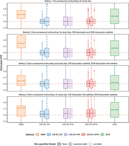
Table 1. Estimated bias, standard error (SE), root mean square error (RMSE), 95% coverage probability, and the average width of a 95% confidence interval, across 3,000 simulations.

Method	Mis-specified Model	Bias	SE	RMSE	Coverage	C.I. Width
Setting 1:
No unmeasured confounding, No study bias
RBMI		0.222	0.189	0.292	84.100	0.828
DID-EC-OR	None	−0.001	0.096	0.096	94.533	0.374
	outcome model	−0.002	0.195	0.195	95.333	0.772
DID-EC-IPW	None	0.003	0.215	0.215	96.233	0.909
	ps model	0.004	0.216	0.215	96.067	0.906
DID-EC-AIPW	None	0.003	0.125	0.125	95.697	0.498
	outcome model	0.002	0.202	0.202	95.626	0.824
	ps model	0.001	0.122	0.122	94.991	0.491
SCM		0.163	0.347	0.383	91.204	1.378
Setting 2:
Exist unmeasured confounding, No study bias, DID Assumption and SCM Assumption satisfied
RBMI		0.319	0.244	0.401	61.600	0.848
DID-EC-OR	None	−0.001	0.111	0.111	94.733	0.441
	outcome model	0.001	0.203	0.203	95.067	0.801
DID-EC-IPW	None	0.000	0.216	0.216	95.933	0.904
	ps model	0.001	0.216	0.216	95.833	0.901
DID-EC-AIPW	None	0.004	0.138	0.138	94.603	0.537
	outcome model	0.001	0.214	0.214	94.674	0.845
	ps model	0.003	0.138	0.138	94.074	0.533
SCM		0.144	0.345	0.374	92.813	1.391
Setting 3:
Exist unmeasured confounding and study bias, DID Assumption satisfied, SCM Assumption Not satisfied
RBMI		0.067	0.237	0.246	89.567	0.838
DID-EC-OR	None	0.003	0.112	0.112	94.733	0.441
	outcome model	−0.004	0.204	0.204	94.733	0.801
DID-EC-IPW	None	−0.001	0.220	0.220	95.900	0.899
	ps model	−0.001	0.221	0.221	95.500	0.894
DID-EC-AIPW	None	0.002	0.136	0.136	94.321	0.538
	outcome model	0.002	0.210	0.210	94.991	0.843
	ps model	0.001	0.136	0.136	94.533	0.536
SCM		0.040	0.347	0.349	94.508	1.387
Setting 4:
Exist unmeasured confounding, No study bias, DID Assumption Not satisfied, SCM Assumption satisfied
RBMI		0.112	0.272	0.294	93.567	0.910
DID-EC-OR	None	0.032	0.137	0.141	94.067	0.539
	outcome model	0.030	0.222	0.224	94.267	0.861
DID-EC-IPW	None	0.050	0.237	0.242	95.167	0.971
	ps model	0.051	0.237	0.243	94.867	0.967
DID-EC-AIPW	None	0.054	0.164	0.172	93.157	0.641
	outcome model	0.054	0.229	0.235	94.674	0.916
	ps model	0.054	0.162	0.171	92.945	0.635
SCM		0.165	0.357	0.393	90.657	1.412

Setting 1 represents the most ideal and less plausible situation where the no unmeasured confounding and no study bias assumptions are valid. In theory, this setting can be handled by methods based on ignorability, such as g-formula, the inverse probability weighting (IPW), and the augmented inverse probability weighting (AIPW). The three DID estimators under correct model specifications all have close to zero bias in finite samples, while the SCM has non negligible bias and RBMI has the largest bias. The DID estimators also have smaller SE and RMSE compared with SCM and RBMI, and have reached nominal coverage probability, while SCM is slightly off and RBMI is more severe.

Setting 2 represents a slightly more plausible situation where investigators might be unaware of some confounder(s) that satisfies Eq. 2 in the DID Assumption 3 without the study bias term, which is also a special case of Eq. 6 in the SCM Assumption 4. The performance metrics are similar to setting 1.

Setting 3 moves beyond setting 2 by allowing a direct effect of trial participation, i.e. study bias, so that satisfies Eq. 2 in the DID Assumption 3, but no longer satisfies Eq. 6 in the SCM Assumption 4. It is possible for unmeasured confounding bias and study bias to be in opposite directions, thereby neutralizing each out, as seen in this simulation setting 3. As a result, SCM may perform numerically better. However, if the two biases are synergistic, SCM’s performance could deteriorate. In Appendix D, we present an additional scenario for setting 3, where the study bias, suggested by the observed data, is not fully canceling out the unmeasured confounding bias. In this scenario, SCM’s performance is consistent.

It is possible for unmeasured confounding bias and study bias to be in opposite directions, thereby canceling each other out, as observed in this simulation. As a result, SCM may perform better than in setting 2, where the unmeasured confounding bias is more pronounced. However, if the two biases are synergistic, SCM’s performance could deteriorate. In Appendix D, we introduce additional simulations for setting 3, where the study bias, suggested by the observed data, is close to 0. In this scenario, SCM’s performance is similar to, if not worse than, that in setting 2

Setting 4 moves beyond setting 2 by allowing the coefficient associated with the unmeasured confounding to be time-varying, so that satisfies Eq. 6 in the SCM Assumption 4, but no longer satisfies Eq. 2 in the DID Assumption 3. In this case, DID estimators show increased bias but are still lower than that of SCM and RBMI.

Nested within each setting, we notice that the effect of model mis-specification is less notable. Mis-specification of outcome tends to increase the SE more than propensity score model mis-specification, while both do not increase bias significantly.

In all four settings, the three DID estimators consistently outperform others on the basis of bias, SE, RMSE, coverage and length of the confidence interval. SCM has noticeable bias, larger SE, wider confidence intervals, and below nominal coverage. In comparison, RBMI performs even worse than both DID and SCM estimators.

Interestingly, even in setting 4, where the SCM Assumption 4 is met but the DID Assumption 3 isn’t, DID methods still surpass SCM. This aligns with our theoretical expectations. The bias of SCM is shown to vanish if (1) the number of first phase time points is large relative to the scale of the error term, which is not likely to hold in settings with limited follow-up visits, such as 2 visits in the randomized controlled phase of SUNFISH trial; and (2) when estimated weights can produce synthetic controls that are a perfect or good match for the respective RCT control patient (Abadie 2021; Abadie et al. 2010). Though DID methods seem to have a more strict assumption, as in the linear model 2 which is a special case satisfying assumption 3, they can still be considered good approximations for settings with slight deviation, as demonstrated in setting 4. In addition, DID methods are computationally more efficient than SCM.

Consequently, we conclude that DID methods are preferred over SCM, and both are preferred over RBMI, for our problem setting. Among the three DID variants, DID-EC-IPW tends to have larger SE than others, while DID-EC-OR and DID-EC-AIPW demonstrate similar finite sample performance. The variance of propensity score weighting estimators has been studied in the literature (Kranker et al. 2021; Zubizarreta 2015), showing that highly variable weights increase the variance of treatment effect estimate, and IPW estimators have seen larger variance compared to the doubly robust (DR) and the outcome regression (OR) approaches (Bang and Robins 2005). When the two groups are imbalanced in terms of measured confounders, the propensity score weights tend to have high variability.

We present additional simulations with a higher percentage of trial controls, where the ratio $n_1:n_0$ is approximately $1:1$ instead of $2:1$, in Appendix E as a sensitivity analysis. The results are consistent with the main simulation results.

5. Application: SUNFISH trial

In this section, we aim to illustrate the application of the proposed methods in Section 3 to the SUNFISH study. The goal is to compare the proposed methods in assessing the long-term efficacy of risdplam during the post primary endpoint, i.e. period II of 12–24 months since the initialization of the study, in the absence of a control group. We augment the SUNFISH trial with external control patients from the olesoxime trial.

Figure 4 displays the balance in baseline covariates between the SUNFISH trial and external controls. The left panel highlights the differences in patient age, Scoliosis, and SMN2 copy number between the two populations. The right panel shows that the propensity scores largely overlap between the two populations, with small regions of non-overlap at both extreme ends, indicating the presence of a few patients in both studies without similar counterparts in the other based on measured covariates. The adjusted sample using the propensity score (covariates enter the propensity score model linearly) demonstrates improved balance, as indicated by the absolute standardized mean difference below the 0.1 threshold (a rough measure of balance).

Figure 5 and Table 2 present the estimated ATE for the SUNFISH population and 95% confidence intervals of the proposed methods, along with the results from a mixed effects model for repeated measures (MMRM) considering the entire 2-year period (period I and II combined), ignoring the fact that the original control arm received treatment after the primary endpoint. Therefore, this analysis during period II (i.e. Naive Comparison) does not align with the estimand of interest, and we use it here simply as a reference to illustrate the consequence of inappropriate analysis.

The native comparison from MMRM during period II shows almost no increase in the benefit of taking risdiplam after the primary endpoint, which is likely to be an underestimate of the long-term benefit as the comparison group were treated. The RBMI estimates are similar to the naive comparison. In contrast, the DID-EC-OR, DID-EC-OR, DID-EC-AIPW, and SCM methods estimate a consistent pattern of continued increase in treatment effect during year 1–2 and therefore show the long-term benefit of taking risdiplam continuously (at least over 2 years). During period II, the external control patients exhibited a declining trend in their observed outcome trajectory (Bertini et al. 2017). In contrast, the trial control group who received treatment during period II showed a relatively stable outcome trajectory (Oskoui et al. 2023). Therefore, a simplistic comparison using the trial control group as the sole reference may underestimate the true treatment effect of risdplam during period II. Using external controls and making appropriate adjustments can provide a more accurate estimate of the treatment effect. Proper adjustment using our proposed methods, i.e. DID and SCM, can mitigate bias when using external controls arise from mechanisms illustrated in Figure 1.

Lastly, note that the schedules of assessment for the SUNFISH trial and the external controls are not exactly matched. In this application, we treated the week 35 in SUNFISH as the same analysis time point as the week 26 in the external controls, assuming that the impact from the time difference is negligible. However, it may not always be the case in practice. One should review the schedule of assessment prior to conducting the analysis and bridging methods may be required. The analysis will benefit from early planning and make sure the trial and external control endpoint assessment frequency are aligned when it is also scientifically rational.

Figure 4. Balance in baseline measured covariates (left panel) and balance in propensity score (right panel).

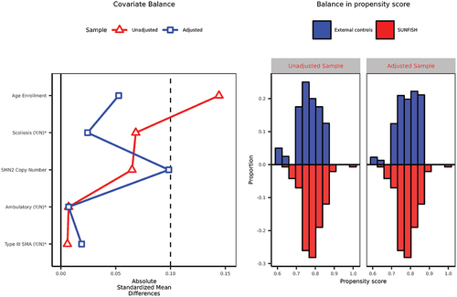
Figure 5. Estimated ATEs for the SUNFISH population and 95% confidence intervals using SUNFISH and external controls combined data. The “RCT results” (solid black line) is a comparison between the two arms of the SUNFISH trial: the risdiplam and the original control group, until week 52. After week 52, the “naive comparison” (black dashed line) is a comparison between the same two groups. Both the “RCT results” and “naive comparison” are obtained using a MMRM, which includes baseline covariates, time (categorized), treatment group, and the interaction between time and treatment group, and is estimated using only the SUNFISH trial data. RBMI, DID-EC-OR, DID-EC-IPW, DID-EC-AIPW and SCM results are estimated using the SUNFISH and the external controls combined data, however, the SUNFISH control patients’ observed outcomes during period II were not used in any of the methods.

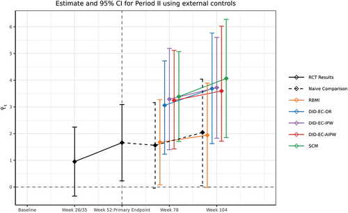
Table 2. Estimated ATEs for the SUNFISH population post primary endpoint.

	Week 78			Week 104
	$\hat{\tau }$	SE	95% C.I.	$\hat{\tau }$	SE	95% C.I.
Naive Comparison	1.562	0.817	(−0.041, 3.164)	2.044	1.018	(0.049, 4.039)
RBMI	1.674	0.806	(0.077, 3.271)	1.941	0.986	(−0.012, 3.893)
DID-EC-OR	3.059	0.988	(1.218, 5.022)	3.685	1.133	(1.570, 6.037)
DID-EC-IPW	3.290	0.946	(1.463, 5.160)	3.721	0.965	(1.964, 5.711)
DID-EC-AIPW	3.246	0.930	(1.363, 5.114)	3.596	1.124	(1.607, 5.935)
SCM	3.387	0.845	(1.732, 5.042)	4.066	1.048	(2.011, 6.121)

6. Discussion

In this article, we consider a methodological challenge encountered in a trial design that allows the control group to crossover to the experimental treatment after reaching the primary endpoint or a pre-determined time, resulting in the absence of a comparison group for evaluating the long-term treatment effect. This design is commonly found in phase III randomized, placebo-controlled studies that include an open-label extension phase, which allows for the assessment of long-term safety and effectiveness while maintaining practicality. To compensate for the lack of a comparison group in the trial for the long-term outcome after switching, we augment the RCT data with appropriately chosen external controls. We have proposed the difference-in-differences (DID) framework and the synthetic control method (SCM) framework for analyzing externally controlled trials, within the causal inference framework. Our proposal complements the literature on externally controlled trials in an RCT with an open-label extension, and also complements the literature on combining experimental and observational data beyond ignorability assumption. Furthermore, we broaden the use of the DID and SCM frameworks, traditionally employed primarily in social sciences, to encompass clinical trials.

The fundamental challenge is that the counterfactual never-treated outcomes for trial patients during the open-label extension phase is unobservable due to switching initial control arm to be treated in the open-label extension phase. To estimate this unobservable counterfactual quantity using the observed outcomes of the external control patients during the same period can result in bias, which only disappears under the ignorability assumption. This assumption is violated in the presence of unmeasured confounding and study bias, as illustrated in Figure 1 by the unblocked back-door path $\mathit{S}\leftarrow \mathit{U}\to {\mathbf{Y}}_{\mathit{II}}$ and a front-door path $\mathit{S}\to {\mathbf{Y}}_{\mathit{II}}$, imply that trial patients and external control patients are not exchangeable, given the measured characteristics. In practical scenarios, being unaware of or unable to obtain certain confounding factors from both data sources can lead to unmeasured confounding bias. Additionally, any systematic differences in outcome measurement between the trial and external controls, such as the placebo effect, can introduce study bias. For a comprehensive discussion on potential sources of bias associated with the use of external controls, refer to (Burger et al. 2021).

Our work relaxes the overly restrictive but commonly used ignorability assumption and proposes methods to adjust for unmeasured confounding bias and study bias. The DID framework relaxes it with the DID Assumption 3. The basic idea is to use the randomized controlled phase outcome as a negative control to de-bias the residual confounding. A special example allows for unmeasured confounding and study bias is shown in Eq. 2. The SCM framework moves beyond the ignorability assumption by allowing for the existence of unmeasured confounding with time-varying coefficients, but not study bias, as shown in Eq. 6 in Assumption 4. The SCM estimation strategy is to find a weighted average of external control patients that matches with each trial control patient in terms of the first phase outcomes and baseline covariates. It has been shown in prior literature that even when perfect match can be found, the bias of SCM estimate goes to zero when the number of first phase time points is large relative to the scale of the error term, which is not likely to hold in settings with limited follow-up visits. The two frameworks, though can be used in similar settings, are based on non-nested assumptions and distinct estimation strategies.

The selection of suitable external controls must be approached with caution to mitigate potential biases. The Pocock criteria (Pocock 1976) is commonly used to evaluate the comparability between external controls and current trials. Additionally, FDA recently released some guidelines for assessing the comparability of external controls (FDA 2023).

We have conducted extensive simulations to compare the performance of the methods proposed. Across all settings, we found that the DID estimators generally produce negligible bias in finite samples, while SCM tends to have noticeable bias. This is consistent with our expectations for several reasons. The DID estimators are consistent if the DID assumption 3 is satisfied, meaning they are unbiased asymptotically, as stated in Theorem 1. In contrast, SCM does not inherently possess an unbiasedness property. The bias in SCM diminishes only under certain conditions: (a) when there is a sufficiently large number of first phase time points relative to the scale of the error term, a condition unlikely to be met in settings with limited follow-up visits such as the randomized controlled phase of the SUNFISH trial featuring only two visits; and (b) when the estimated weights generate synthetic controls closely matching the respective RCT control patients (Abadie 2021; Abadie et al. 2010). Neither condition is commonly satisfied in practice. While DID methods might appear to impose stricter assumptions, particularly in the linear model referenced in Eq. 2—which is a special case meeting the DID assumption 3—they still serve as good approximations even when these assumptions are slightly violated, as evidenced in setting 4. In summary, the DID framework outperforms SCM across various metrics including bias, Root Mean Square Error (RMSE), coverage, confidence interval length, and computational time. Therefore, we recommend the DID framework as the method of choice over SCM. Certainly, if both the DID and SCM methods yield consistent results, this would offer an additional layer of reassurance regarding the robustness and validity of the findings, as our findings for the SUNFISH trial in Section 5.

For future research, we will consider extending the proposed framework in the following directions. (1) We will consider extending the DID and SCM framework to accommodate more flexible longitudinal data structure. (2) The DID estimators require the estimation of either the outcome model or propensity of trial participation model, or both, and their performances are dependent on the ability to have correct models for these nuisance parameters. This is especially challenging in the presence of high-dimensional baseline covariates, one needs to go beyond parametric models. We will also consider the incorporation of machine learning in the DID framework.

We hope our proposed methods offer strategies to the analysis of long-term outcomes by augmenting the trial data with real-world data, such as external controls, enrich the literature in the current topic of external controls in clinical trials, and stimulate further investigation.

Ethics approvals

De-identified SUNFISH data was used in this statistical methodology study. The SUNFISH study was conducted in accordance with the principles of the Declaration of Helsinki, in full conformance with Good Clinical Practice guidelines, and in accordance with regulations and procedures outlined in the study protocol. The study was approved by the independent research ethics board at each participating site.

Acknowledgements

We would like to express our gratitude to Winnie Yeung and Tammy Mclver who provided valuable insights and expertise that greatly assisted the research.

Disclosure statement

Drs Pang, Burger, and Zhu are employees of Genentech/Roche. They own Roche stocks. However, the published work is methodology focused.

Additional information

Funding

This work is partially supported by a grant from the FDA (HHS U01 FD007206, Pang and Zhu).

Appendix A.

Remark 6. Assumption 3 is a causal assumption that describes relationship between potentially unobserved counterfactual outcomes, making it unverifiable in practice. However, we can assess its plausibility by comparing trial control patients and external control patients during the randomized placebo-controlled period I. This comparison can be facilitated through a regression model incorporating measured covariates, trial participation, time, and an interaction between trial participation and time. If the interaction term proves insignificant, it lends some credibility to Assumption 3. Nevertheless, it’s important to note that this only suggests the plausibility of the assumption during the time period for which data is available. It doesn’t directly validate the assumption’s plausibility during the open-label extension period, which is our primary area of interest.

Remark 7. Assumption 3 offers a mechanism to estimate the residual bias by leveraging the existence of the first randomized controlled period. If satisfied, this assumption results in unbiased estimators. Despite being unverifiable, if one deems this assumption approximately reasonable, it can be viewed as an approximation to the unknowable bias term. Consequently, the resulting estimators can be interpreted as approximations to the average treatment effect.

Remark 8. The non-negative and sum-to-one constraints in the SC weights are proposed, similarly as the matching estimators, to minimize extrapolation bias. Ideally, the observed characteristics of a trial control patient should reside inside the convex null of few external controls, which avoids the danger of extrapolation. And the penalization of pairwise discrepancies further minimizes the danger of interpolation bias.

Remark 9. Though the difference-in-differences methods and synthetic control methods have different assumptions and approach the counterfactual estimation problem differently, both can be viewed as special types of regression estimators, as both are in the form of linear combinations of external controls. Refer to the observed and missing outcome structure in Eq. ?, both can be viewed as “vertical regression” with different constraints, where we treat the external control outcomes across patients as predictors and across time as repeated observations (Doudchenko and Imbens 2016). The regression formulation corresponding to the original SCM (Abadie et al. 2010) has one distinctive constraint – no intercept. From the pure statistical model perspective, they are different constrained regression models. From the causal perspective, the constraints have substantive interpretations: the no-intercept constraint of SCM does not allow for study effect or a direct effect of trial participation on outcomes outside of treatment, which is an important feature of DID methods which assume that the never-treated outcomes of the trial controls and external controls can be systematically different as long as this gap is constant over time.

Appendix B.

Let $\mathit{g}(\mathit{O};\mathit{\theta })$ be a generic notation for parametric models ${\pi }_S(\mathit{X};\mathit{\beta })$ and $\mathit{\mu }(\mathit{t},\mathit{S},\mathbf{A},\mathit{X};\mathit{\gamma })$, where $\mathit{O}$ stands for relevant variables used in generic model $\mathit{g}$. Assumption 5 requires that the models for the nuisance components to be smooth parametric models. These requirements are standard and satisfied when the outcome regression and propensity score models are estimated by least squares or maximum likelihood methods.

Assumption 5.

$\mathit{g}(\mathit{x})=\mathit{g}(\mathit{x};\mathit{\theta })$ is a parametric model, where $\mathit{\theta }\in \mathrm{\Theta }\subset {\mathbb{R}}^k,\mathrm{\Theta }$ being compact, and

1. $\mathit{g}(\mathit{X};\mathit{\theta })$ is a.s. continuous at each $\mathit{\theta }\in \mathrm{\Theta }$;

2. there exists a unique pseudo-true parameter ${\theta }^{\ast }\in$ int $(\mathrm{\Theta })$;

3. the estimator $\hat{\theta }$ is consistent for the ${\theta }^{\ast }$.

Proof (Equation 3). ${\mathbb{E}}_{\mathcal{R}}\left[Y_t^{(1,(1,1))}\right]$ is directly estimable from the trial treated patients. Under the assumption 2,

${\mathbb{E}}_{\mathcal{R}}\left[Y_t^{(1,(1,1))}\right]={\mathbb{E}}_{\mathbf{X}|\mathcal{R}}\left[\mathbb{E}\left[Y_t|\mathbf{X},\mathit{S}=1,A_1=1\right]\right]$

The external controls can be used to identify ${\mathbb{E}}_{\mathcal{R}}\left[Y_t^{(1,(0,0))}\right]$, provided that the assumption 3 holds,

${\mathbb{E}}_{\mathcal{R}}\left[Y_t^{(1,(0,0))}\right]={\mathbb{E}}_{\mathbf{X}|\mathcal{R}}\left[\mathbb{E}\left(Y_t^{(1,(0,0))}|\mathbf{X}\right)\right]$

$={\mathbb{E}}_{\mathbf{X}|\mathcal{R}}\left[\mathbb{E}\left(Y_t^{(0,(0,0))}|\mathbf{X}\right)+\mathit{B}(\mathbf{X})\right]$

$={\mathbb{E}}_{\mathbf{X}|\mathcal{R}}\left[\mathbb{E}\left(Y_t|\mathbf{X},\mathit{S}=0,\mathbf{A}=(0,0)\right)+\mathit{B}(\mathbf{X})\right]$

The constant conditional bias $\mathit{B}(\mathbf{X})$ can be estimated under assumption 3, as long as there exists a period I (even a single measurement is enough) during which the trial control patients were not treated, so that the difference between the trial controls and external controls at those time points quantify the unmeasured conditional bias, and we can use the estimated conditional bias to de-bias the period II of interest. This idea is intuitively illustrated as the parallel trend in Figure 1. A simple strategy to pool the differences observed in multiple period I time points is an average difference:

$\mathit{B}(\mathbf{X})=\frac{1}{T_1}\sum _{\mathit{t}\in {\mathcal{T}}_1}\left({\mathbb{E}}_{\mathcal{R}}\left[Y_t^{(1,(0))}|\mathbf{X}\right]-{\mathbb{E}}_{\mathcal{E}}\left[Y_t^{(0,(0))}|\mathbf{X}\right]\right)$

$=\frac{1}{T_1}\sum _{\mathit{t}\in {\mathcal{T}}_1}\left(\mathbb{E}\left[Y_t|\mathbf{X},\mathit{S}=1,A_1=0\right]-\mathbb{E}\left[Y_t|\mathbf{X},\mathit{S}=0,A_1=0\right]\right)$

Put it together, the estimand in Eq. 1 can be identified by

${\tau }_t={\mathbb{E}}_{\mathcal{R}}\left[\left(\mathit{\mu }(\mathbf{X},\mathit{S}=1,\mathbf{A}=(1,1),\mathit{t})-\bar{\mu }(\mathbf{X},\mathit{S}=1,A_1=0,{\mathcal{T}}_1)\right)\right.$

$\left.-\left(\mathit{\mu }(\mathbf{X},\mathit{S}=0,\mathbf{A}=(0,0),\mathit{t})-\bar{\mu }(\mathbf{X},\mathit{S}=0,A_1=0,{\mathcal{T}}_1)\right)\right]$

$\mathit{for}\mathit{t}\in {\mathcal{T}}_2.$

Proof (Equation 4). We can also identify the estimand using a weighting approach. Under the assumption 2,

${\mathbb{E}}_{\mathcal{R}}\left[Y_t^{(1,(1,1))}\right]=\frac{{\mathbb{E}}_{\mathcal{R}}\left[\frac{A_1{Y}_t}{{\pi }_A}\right]}{{\mathbb{E}}_{\mathcal{R}}\left[\frac{A_1}{{\pi }_A}\right]}=\frac{{\mathbb{E}}_{\mathcal{R}}\left[A_1{W}_{11}{Y}_t\right]}{{\mathbb{E}}_{\mathcal{R}}\left[A_1{W}_{11}\right]}$

Similarly, provided that the assumption 3 holds,

${\mathbb{E}}_{\mathcal{R}}\left[Y_t^{(1,(0,0))}\right]=\int \mathbb{E}\left[Y_t^{(1,(0,0))}|\mathbf{X}\right]p_{\mathcal{R}}(\mathit{x})\mathit{\mu }(\mathit{dx})$

$=\frac{\int \mathbb{E}\left[Y_t^{(1,(0,0))}|\mathbf{X}\right]\frac{{\mathit{p}}_{\mathcal{R}}(\mathit{x})}{p_{\mathcal{E}}(\mathit{x})}{p}_{\mathcal{E}}(\mathit{x})\mathit{\mu }(\mathit{dx})}{\int \frac{{\mathit{p}}_{\mathcal{R}}(\mathit{x})}{p_{\mathcal{E}}(\mathit{x})}{p}_{\mathcal{E}}(\mathit{x})\mathit{\mu }(\mathit{dx})}$

$=\frac{\int \left(\mathbb{E}\left[Y_t^{(0,(0,0))}|\mathbf{X}\right]+\mathit{B}(\mathbf{X})\right)\frac{{\mathit{p}}_{\mathcal{R}}(\mathit{x})}{p_{\mathcal{E}}(\mathit{x})}{p}_{\mathcal{E}}(\mathit{x})\mathit{\mu }(\mathit{dx})}{\int \frac{{\mathit{p}}_{\mathcal{R}}(\mathit{x})}{p_{\mathcal{E}}(\mathit{x})}{p}_{\mathcal{E}}(\mathit{x})\mathit{\mu }(\mathit{dx})}$

$=\frac{{\mathbb{E}}_{\mathcal{E}}[W_0(\mathbf{X})\left(Y_t+\mathit{B}(\mathbf{X})\right)]}{{\mathbb{E}}_{\mathcal{E}}[W_0(\mathbf{X})]}$

The constant conditional bias $\mathit{B}(\mathbf{X})$ can be estimated similarly

$\mathit{B}(\mathbf{X})=\frac{1}{T_1}\sum _{\mathit{t}\in {\mathcal{T}}_1}\left(\mathbb{E}\left[Y_t^{(1,(0,0))}|\mathbf{X}\right]-\mathbb{E}\left[Y_t^{(0,(0,0))}|\mathbf{X}\right]\right)$

Put it together, the estimand in Eq. 1 can be identified by

${\tau }_t=\frac{{\mathbb{E}}_{\mathcal{R}}\left[A_1{W}_{11}{Y}_t\right]}{{\mathbb{E}}_{\mathcal{R}}\left[A_1{W}_{11}\right]}-\frac{{\mathbb{E}}_{\mathcal{E}}[W_0(\mathbf{X})\left(Y_t^{(0,(0,0))}+\frac{1}{T_1}{\sum }_{\mathit{t}\in {\mathcal{T}}_1}\left(\mathbb{E}\left[Y_t^{(1,(0,0))}|\mathbf{X}\right]-\mathbb{E}\left[Y_t^{(0,(0,0))}|\mathbf{X}\right]\right)\right)]}{{\mathbb{E}}_{\mathcal{E}}[W_0(\mathbf{X})]}$

$={\mathbb{E}}_{\mathcal{R}}\left[\frac{A_1{W}_{11}}{{\mathbb{E}}_{\mathcal{R}}\left[A_1{W}_{11}\right]}{Y}_t-\frac{(1-A_1)W_{10}}{{\mathbb{E}}_{\mathcal{R}}\left[(1-A_1)W_{10}\right]}\bar{Y}({\mathcal{T}}_1)\right]$

$-{\mathbb{E}}_{\mathcal{E}}\left[\frac{W_0(\mathbf{X})}{{\mathbb{E}}_{\mathcal{E}}\left[W_0(\mathbf{X})\right]}\left(Y_t-\bar{Y}({\mathcal{T}}_1)\right)\right]$

$\mathit{for}\mathit{t}\in {\mathcal{T}}_2.$

Proof (Equation 5).

${\tau }_t^{\mathrm{D}\mathrm{I}\mathrm{D}-\mathrm{E}\mathrm{C}-\mathrm{A}\mathrm{I}\mathrm{P}\mathrm{W}}={\tau }_t^{\mathrm{D}\mathrm{I}\mathrm{D}-\mathrm{E}\mathrm{C}-\mathrm{I}\mathrm{P}\mathrm{W}}$

$-{\mathbb{E}}_{\mathcal{R}}\left[\frac{A_1{W}_{11}}{{\mathbb{E}}_{\mathcal{R}}\left[A_1{W}_{11}\right]}\mathit{\mu }(\mathbf{X},\mathit{S}=0,\mathit{A}=0,\mathit{t})-\frac{(1-A_1)W_{10}}{{\mathbb{E}}_{\mathcal{R}}\left[(1-A_1)W_{10}\right]}\bar{\mu }(\mathbf{X},\mathit{S}=0,\mathit{A}=0,{\mathcal{T}}_1)\right]$

$-{\mathbb{E}}_{\mathcal{E}}\left[\frac{W_0(\mathbf{X})}{{\mathbb{E}}_{\mathcal{E}}\left[W_0(\mathbf{X})\right]}\left(\mathit{\mu }(\mathbf{X},\mathit{S}=0,\mathit{A}=0,\mathit{t})-\bar{\mu }(\mathbf{X},\mathit{S}=0,\mathit{A}=0,{\mathcal{T}}_1)\right)\right]$

$={\tau }_t^{\mathrm{D}\mathrm{I}\mathrm{D}-\mathrm{E}\mathrm{C}-\mathrm{I}\mathrm{P}\mathrm{W}}$

$-{\mathbb{E}}_{\mathcal{R}}\left[\mathit{\mu }(\mathbf{X},\mathit{S}=0,\mathit{A}=0,\mathit{t})-\bar{\mu }(\mathbf{X},\mathit{S}=0,\mathit{A}=0,{\mathcal{T}}_1)\right]$

$-{\mathbb{E}}_{\mathcal{R}}\left[\mathit{\mu }(\mathbf{X},\mathit{S}=0,\mathit{A}=0,\mathit{t})-\bar{\mu }(\mathbf{X},\mathit{S}=0,\mathit{A}=0,{\mathcal{T}}_1)\right]$

$={\tau }_t^{\mathrm{D}\mathrm{I}\mathrm{D}-\mathrm{E}\mathrm{C}-\mathrm{I}\mathrm{P}\mathrm{W}}={\tau }_t$

$\mathit{for}\mathit{t}\in {\mathcal{T}}_2.$

Plug in the estimated nuisance parameters and replace the expectations with sample average, the three variants of DID type estimators, ${\hat{\tau }}_{\mathit{t}}^{\mathrm{DID}-\mathrm{EC}-\mathrm{OR}}$, ${\hat{\tau }}_{\mathit{t}}^{\mathrm{DID}-\mathrm{EC}-\mathrm{IPW}}$, and ${\hat{\tau }}_{\mathit{t}}^{\mathrm{DID}-\mathrm{EC}-\mathrm{AIPW}}$:

${\hat{\tau }}_{\mathit{t}}^{\mathrm{DID}-\mathrm{EC}-\mathrm{OR}}=\frac{1}{n}\sum _{\mathit{i}\in \mathcal{R}}\underset{{\mathrm{\Delta }}_{\mathit{trial}}}{\underbrace{\left(\mathit{\mu }({\mathbf{X}}_i,S_i=1,{\mathbf{A}}_i=(1,1),\mathit{t})-\bar{\mu }({\mathbf{X}}_i,S_i=1,A_{\mathit{i}1}=0,{\mathcal{T}}_1)\right)}}$

$-\underset{{\mathrm{\Delta }}_{\mathit{EC}}}{\underbrace{\left(\mathit{\mu }({\mathbf{X}}_i,S_i=0,{\mathbf{A}}_i=(0,0),\mathit{t})-\bar{\mu }({\mathbf{X}}_i,S_i=0,A_{\mathit{i}1}=0,{\mathcal{T}}_1)\right)}}$

${\hat{\tau }}_{\mathit{t}}^{\mathrm{DID}-\mathrm{EC}-\mathrm{IPW}}=\underset{{\mathrm{\Delta }}_{\mathit{trial}}}{\underbrace{\sum _{\mathit{i}\in \mathcal{R}}\left[\frac{{\mathit{A}}_{\mathit{i}1}{\hat{W}}_{11}}{{\sum }_{\mathit{i}\in \mathcal{R}}{A}_{\mathit{i}1}{\hat{W}}_{11}}{Y}_{\mathit{it}}-\frac{(1-{\mathit{A}}_{\mathit{i}1}){\hat{W}}_{10}}{{\sum }_{\mathit{i}\in \mathcal{R}}(1-A_{\mathit{i}1}){\hat{W}}_{10}}{\bar{Y}}_{\mathit{i}}({\mathcal{T}}_1)\right]}}$

$-\underset{{\mathrm{\Delta }}_{\mathit{EC}}}{\underbrace{\sum _{\mathit{i}\in \mathcal{E}}\left[\frac{{\hat{W}}_0({\mathbf{X}}_i)}{{\sum }_{\mathit{i}\in \mathcal{E}}{\hat{W}}_0({\mathbf{X}}_i)}\left(Y_{\mathit{it}}-{\bar{Y}}_{\mathit{i}}({\mathcal{T}}_1)\right)\right]}}$

${\hat{\tau }}_{\mathit{t}}^{\mathrm{DID}-\mathrm{EC}-\mathrm{AIPW}}=\underset{{\mathrm{\Delta }}_{\mathit{trial}}}{\underbrace{\sum _{\mathit{i}\in \mathcal{R}}\left[\frac{{\mathit{A}}_{\mathit{i}1}{\hat{W}}_{11}}{{\sum }_{\mathit{i}\in \mathcal{R}}{A}_{\mathit{i}1}{\hat{W}}_{11}}{\hat{\tilde{Y}}}_{\mathit{it}}-\frac{(1-{\mathit{A}}_{\mathit{i}1}){\hat{W}}_{10}}{{\sum }_{\mathit{i}\in \mathcal{R}}(1-A_{\mathit{i}1}){\hat{W}}_{10}}{\widehat{\stackrel{‾}{\tilde{Y}}}}_{\mathit{i}}({\mathcal{T}}_1)\right]}}$

$-\underset{{\mathrm{\Delta }}_{\mathit{EC}}}{\underbrace{\sum _{\mathit{i}\in \mathcal{E}}\left[\frac{{\hat{W}}_0}{{\sum }_{\mathit{i}\in \mathcal{E}}{\hat{W}}_0}\left({\hat{\tilde{Y}}}_{\mathit{it}}-\stackrel{ˆ}{{\bar{\tilde{Y}}}_{\mathit{i}}}({\mathcal{T}}_1)\right)\right]}}$

where the estimated nuisance components are plugged in and indicated by the hats.

Appendix C.

Proof (1). (a) If the outcome model is correctly specified, i.e. $\mathit{\mu }(\mathbf{X},\mathit{S},\mathit{A},\mathit{t};{\gamma }^{\ast })=\mathit{\mu }(\mathbf{X},\mathit{S},\mathit{A},\mathit{t})$, and it satisfies assumption 5, by the continuous mapping theorem and the weak law of large numbers, we have

${\hat{\mu }}_{\mathit{S}}(\mathbf{X},\mathit{S},\mathit{A},\mathit{t};\hat{\gamma })\stackrel{p}{⟶}\mathit{\mu }(\mathbf{X},\mathit{S},\mathit{A};{\gamma }^{\ast })=\mathit{\mu }(\mathbf{X},\mathit{S},\mathit{A},\mathit{t})$

Then,

${\hat{\tau }}_{\mathit{t}}^{\mathrm{DID}-\mathrm{EC}-\mathrm{OR}}=\frac{1}{n}\sum _{\mathit{i}\in \mathcal{R}}\left[\left(\hat{\mu }({\mathbf{X}}_i,S_i=1,{\mathbf{A}}_i=(1,1),\mathit{t})-\overline{\stackrel{ˆ}{\mu }}({\mathbf{X}}_i,S_i=1,A_{\mathit{i}1}=0,{\mathcal{T}}_1)\right)\right.$

$\left.-\left(\hat{\mu }({\mathbf{X}}_i,S_i=0,{\mathbf{A}}_i=(0,0),\mathit{t})-\overline{\stackrel{ˆ}{\mu }}({\mathbf{X}}_i,S_i=0,A_{\mathit{i}1}=0,{\mathcal{T}}_1)\right)\right]$

$\stackrel{p}{⟶}{\mathbb{E}}_{\mathcal{R}}\left[\left(\mathit{\mu }(\mathbf{X},\mathit{S}=1,\mathbf{A}=(1,1),\mathit{t};{\gamma }^{\ast })-\bar{\mu }(\mathbf{X},\mathit{S}=1,A_1=0,{\mathcal{T}}_1;{\gamma }^{\ast })\right)\right.$

$\left.-\left(\mathit{\mu }(\mathbf{X},\mathit{S}=0,\mathbf{A}=(0,0),\mathit{t};{\gamma }^{\ast })-\bar{\mu }(\mathbf{X},\mathit{S}=0,A_1=0,{\mathcal{T}}_1;{\gamma }^{\ast })\right)\right]$

$={\tau }_t^{\mathrm{D}\mathrm{I}\mathrm{D}-\mathrm{E}\mathrm{C}-\mathrm{O}\mathrm{R}}={\tau }_t$

$\mathit{t}\in {\mathcal{T}}_2.$

(b) If the propensity of trial participation model is correctly specified, i.e. ${\pi }_S(\mathbf{X};{\beta }^{\ast })={\pi }_S(\mathbf{X})$, and it satisfies assumption 5, by the continuous mapping theorem and the weak law of large numbers, we have

${\hat{\pi }}_{\mathit{S}}(\mathbf{X};\hat{\beta })\stackrel{p}{⟶}{\pi }_S(\mathbf{X};{\beta }^{\ast })={\pi }_S(\mathbf{X})$

Then,

${\hat{\tau }}_{\mathit{t}}^{\mathrm{DID}-\mathrm{EC}-\mathrm{IPW}}=\sum _{\mathit{i}\in \mathcal{R}}\left[\frac{{\mathit{A}}_{\mathit{i}1}{\hat{W}}_{11}}{{\sum }_{\mathit{i}\in \mathcal{R}}{A}_{\mathit{i}1}{\hat{W}}_{11}}{Y}_{\mathit{it}}-\frac{(1-{\mathit{A}}_{\mathit{i}1}){\hat{W}}_{10}}{{\sum }_{\mathit{i}\in \mathcal{R}}(1-A_{\mathit{i}1}){\hat{W}}_{10}}{\bar{Y}}_{\mathit{i}}({\mathcal{T}}_1)\right]$

$-\sum _{\mathit{i}\in \mathcal{E}}\left[\frac{{\hat{W}}_0({\mathbf{X}}_i)}{{\sum }_{\mathit{i}\in \mathcal{E}}{\hat{W}}_0({\mathbf{X}}_i)}\left(Y_{\mathit{it}}-{\bar{Y}}_{\mathit{i}}({\mathcal{T}}_1)\right)\right]$

$\stackrel{p}{⟶}{\mathbb{E}}_{\mathcal{R}}\left[\frac{A_1{W}_{11}}{{\mathbb{E}}_{\mathcal{R}}\left[A_1{W}_{11}\right]}{Y}_t-\frac{(1-A_1)W_{10}}{{\mathbb{E}}_{\mathcal{R}}\left[(1-A_1)W_{10}\right]}\bar{Y}({\mathcal{T}}_1)\right]$

$-{\mathbb{E}}_{\mathcal{E}}\left[\frac{W_0(\mathbf{X})}{{\mathbb{E}}_{\mathcal{E}}\left[W_0(\mathbf{X})\right]}\left(Y_t-\bar{Y}({\mathcal{T}}_1)\right)\right]$

$={\tau }_t^{\mathrm{D}\mathrm{I}\mathrm{D}-\mathrm{E}\mathrm{C}-\mathrm{I}\mathrm{P}\mathrm{W}}={\tau }_t$

$\mathit{for}\mathit{t}\in {\mathcal{T}}_2.$

(c) If the assumption 5 holds for both the outcome model and the propensity of trial participation model, by the continuous mapping theorem and the weak law of large numbers, we have

${\hat{\mu }}_{\mathit{S}}(\mathbf{X},\mathit{S},\mathit{A},\mathit{t};\hat{\gamma })\stackrel{p}{⟶}\mathit{\mu }(\mathbf{X},\mathit{S},\mathit{A};{\gamma }^{\ast })$

${\hat{\pi }}_{\mathit{S}}(\mathbf{X};\hat{\beta })\stackrel{p}{⟶}{\pi }_S(\mathbf{X};{\beta }^{\ast })$

${\hat{\tau }}_{\mathit{t}}^{\mathrm{DID}-\mathrm{EC}-\mathrm{AIPW}}=\sum _{\mathit{i}\in \mathcal{R}}\left[\frac{{\mathit{A}}_{\mathit{i}1}{\hat{W}}_{11}}{{\sum }_{\mathit{i}\in \mathcal{R}}{A}_{\mathit{i}1}{\hat{W}}_{11}}{\hat{\tilde{Y}}}_{\mathit{it}}-\frac{(1-{\mathit{A}}_{\mathit{i}1}){\hat{W}}_{10}}{{\sum }_{\mathit{i}\in \mathcal{R}}(1-A_{\mathit{i}1}){\hat{W}}_{10}}{\widehat{\stackrel{‾}{\tilde{Y}}}}_{\mathit{i}}({\mathcal{T}}_1)\right]$

$-\sum _{\mathit{i}\in \mathcal{E}}\left[\frac{{\hat{W}}_0({\mathbf{X}}_i)}{{\sum }_{\mathit{i}\in \mathcal{E}}{\hat{W}}_0({\mathbf{X}}_i)}\left({\hat{\tilde{Y}}}_{\mathit{it}}-{\widehat{\stackrel{‾}{\tilde{Y}}}}_{\mathit{i}}({\mathcal{T}}_1)\right)\right]$

$\stackrel{p}{⟶}{\mathbb{E}}_{\mathcal{R}}\left[\frac{A_1{W}_{11}}{{\mathbb{E}}_{\mathcal{R}}\left[A_1{W}_{11}\right]}{\tilde{Y}}_{\mathit{t}}({\gamma }^{\ast })-\frac{(1-A_1)W_{10}}{{\mathbb{E}}_{\mathcal{R}}\left[(1-A_1)W_{10}\right]}\bar{\tilde{Y}}({\mathcal{T}}_1;{\gamma }^{\ast })\right]$

$-{\mathbb{E}}_{\mathcal{E}}\left[\frac{W_0(\mathbf{X};{\beta }^{\ast })}{{\mathbb{E}}_{\mathcal{E}}\left[W_0(\mathbf{X};{\beta }^{\ast })\right]}\left({\tilde{Y}}_{\mathit{t}}({\gamma }^{\ast })-\bar{\tilde{Y}}({\mathcal{T}}_1;{\gamma }^{\ast })\right)\right]$

Next, we show it has the doubly robust property. If the outcome model is correctly specified, i.e. $\mathit{\mu }(\mathbf{X},\mathit{S},\mathit{A},\mathit{t};{\gamma }^{\ast })=\mathit{\mu }(\mathbf{X},\mathit{S},\mathit{A},\mathit{t})$, then

${\mathbb{E}}_{\mathcal{E}}\left[\frac{W_0(\mathbf{X};{\beta }^{\ast })}{{\mathbb{E}}_{\mathcal{E}}\left[W_0(\mathbf{X};{\beta }^{\ast })\right]}\left({\tilde{Y}}_{\mathit{t}}({\gamma }^{\ast })-\bar{\tilde{Y}}({\mathcal{T}}_1;{\gamma }^{\ast })\right)\right]$

$={\mathbb{E}}_{\mathcal{E}}\left[\frac{W_0(\mathbf{X})}{{\mathbb{E}}_{\mathcal{E}}\left[W_0(\mathbf{X})\right]}\left({\tilde{Y}}_{\mathit{t}}-\bar{\tilde{Y}}({\mathcal{T}}_1)\right)\right]$

$={\mathbb{E}}_{\mathcal{E}}\left[\frac{W_0(\mathbf{X})}{{\mathbb{E}}_{\mathcal{E}}\left[W_0(\mathbf{X})\right]}\left(\mathbb{E}[{\tilde{Y}}_{\mathit{t}}|\mathbf{X},\mathit{S}=0,\mathbf{A}=(0,0),\mathit{t}]-\mathbb{E}[\tilde{Y}({\mathcal{T}}_1)|\mathbf{X},\mathit{S}=0,A_1=0,\mathit{t}]\right)\right]$

$={\mathbb{E}}_{\mathcal{E}}\left[\frac{W_0(\mathbf{X})}{{\mathbb{E}}_{\mathcal{E}}\left[W_0(\mathbf{X})\right]}\left(0-0\right)\right]$

$=0$

and

${\mathbb{E}}_{\mathcal{R}}\left[\frac{A_1{W}_{11}}{{\mathbb{E}}_{\mathcal{R}}\left[A_1{W}_{11}\right]}{\tilde{Y}}_{\mathit{t}}({\mathbf{g}}^{\ast }{\mathbf{y}}^{\ast })-\frac{(1-A_1)W_{10}}{{\mathbb{E}}_{\mathcal{R}}\left[(1-A_1)W_{10}\right]}\bar{\tilde{Y}}({\mathcal{T}}_1;{\gamma }^{\ast })\right]$

$={\mathbb{E}}_{\mathcal{R}}\left[\frac{A_1{W}_{11}}{{\mathbb{E}}_{\mathcal{R}}\left[A_1{W}_{11}\right]}{\tilde{Y}}_{\mathit{t}}-\frac{(1-A_1)W_{10}}{{\mathbb{E}}_{\mathcal{R}}\left[(1-A_1)W_{10}\right]}\bar{\tilde{Y}}({\mathcal{T}}_1)\right]$

$={\mathbb{E}}_{\mathcal{R}}[\left(\mathit{\mu }(\mathbf{X},\mathit{S}=1,\mathbf{A}=(1,1),\mathit{t})-\bar{\mu }(\mathbf{X},\mathit{S}=1,A_1=0,{\mathcal{T}}_1)\right)$

$-\left(\mathit{\mu }(\mathbf{X},\mathit{S}=0,\mathbf{A}=(0,0),\mathit{t})-\bar{\mu }(\mathbf{X},\mathit{S}=0,A_1=0,{\mathcal{T}}_1)\right)]$

$={\tau }_t^{\mathrm{D}\mathrm{I}\mathrm{D}-\mathrm{E}\mathrm{C}-\mathrm{O}\mathrm{R}}={\tau }_t$

Therefore,

${\hat{\tau }}_{\mathit{t}}^{\mathrm{DID}-\mathrm{EC}-\mathrm{AIPW}}\stackrel{p}{⟶}{\tau }_t^{\mathrm{D}\mathrm{I}\mathrm{D}-\mathrm{E}\mathrm{C}-\mathrm{O}\mathrm{R}}={\tau }_t$

On the other hand, if the propensity of trial participation model ${\pi }_S(\mathbf{X};{\beta }^{\ast })={\pi }_S(\mathbf{X})$, then re-arrange

${\mathbb{E}}_{\mathcal{R}}\left[\frac{A_1{W}_{11}}{{\mathbb{E}}_{\mathcal{R}}\left[A_1{W}_{11}\right]}{\tilde{Y}}_{\mathit{t}}({\gamma }^{\ast })-\frac{(1-A_1)W_{10}}{{\mathbb{E}}_{\mathcal{R}}\left[(1-A_1)W_{10}\right]}\bar{\tilde{Y}}({\mathcal{T}}_1;{\gamma }^{\ast })\right]$

$-{\mathbb{E}}_{\mathcal{E}}\left[\frac{W_0(\mathbf{X};{\beta }^{\ast })}{{\mathbb{E}}_{\mathcal{E}}\left[W_0(\mathbf{X};{\beta }^{\ast })\right]}\left({\tilde{Y}}_{\mathit{t}}({\gamma }^{\ast })-\bar{\tilde{Y}}({\mathcal{T}}_1;{\gamma }^{\ast })\right)\right]$

$={\tau }_t^{\mathrm{D}\mathrm{I}\mathrm{D}-\mathrm{E}\mathrm{C}-\mathrm{I}\mathrm{P}\mathrm{W}}$

$-{\mathbb{E}}_{\mathcal{R}}\left[\frac{A_1{W}_{11}}{{\mathbb{E}}_{\mathcal{R}}\left[A_1{W}_{11}\right]}\mathit{\mu }(\mathbf{X},\mathit{S}=0,\mathbf{A}=(0,0),\mathit{t};{\gamma }^{\ast })-\frac{(1-A_1)W_{10}}{{\mathbb{E}}_{\mathcal{R}}\left[(1-A_1)W_{10}\right]}\bar{\mu }(\mathbf{X},\mathit{S}=0,A_1=0;,{\mathcal{T}}_1;{\gamma }^{\ast })\right]$

$+{\mathbb{E}}_{\mathcal{E}}\left[\frac{W_0(\mathbf{X};{\beta }^{\ast })}{{\mathbb{E}}_{\mathcal{E}}\left[W_0(\mathbf{X};{\beta }^{\ast })\right]}\left(\mathit{\mu }(\mathbf{X},\mathit{S}=0,\mathbf{A}=(0,0),\mathit{t};{\gamma }^{\ast })-\bar{\mu }(\mathbf{X},\mathit{S}=0,A_1=0;,{\mathcal{T}}_1;{\gamma }^{\ast })\right)\right]$

$={\tau }_t^{\mathrm{D}\mathrm{I}\mathrm{D}-\mathrm{E}\mathrm{C}-\mathrm{I}\mathrm{P}\mathrm{W}}$

$-{\mathbb{E}}_{\mathcal{R}}\left[\mathit{\mu }(\mathbf{X},\mathit{S}=0,\mathbf{A}=(0,0),\mathit{t};{\gamma }^{\ast })-\bar{\mu }(\mathbf{X},\mathit{S}=0,A_1=0,{\mathcal{T}}_1;{\gamma }^{\ast })\right]$

$+{\mathbb{E}}_{\mathcal{R}}\left[\mathit{\mu }(\mathbf{X},\mathit{S}=0,\mathbf{A}=(0,0),\mathit{t};{\gamma }^{\ast })-\bar{\mu }(\mathbf{X},\mathit{S}=0,\mathbf{A}=(0,0),{\mathcal{T}}_1;{\gamma }^{\ast })\right]$

$={\tau }_t^{\mathrm{D}\mathrm{I}\mathrm{D}-\mathrm{E}\mathrm{C}-\mathrm{I}\mathrm{P}\mathrm{W}}$

Therefore,

${\hat{\tau }}_{\mathit{t}}^{\mathrm{DID}-\mathrm{EC}-\mathrm{AIPW}}\stackrel{p}{⟶}{\tau }_t^{\mathrm{D}\mathrm{I}\mathrm{D}-\mathrm{E}\mathrm{C}-\mathrm{I}\mathrm{P}\mathrm{W}}={\tau }_t$

We have shown it has the doubly robust property that, if either one of the outcome model and the propensity of trial participation model is correctly specified,

${\hat{\tau }}_{\mathit{t}}^{\mathrm{DID}-\mathrm{EC}-\mathrm{AIPW}}\stackrel{p}{⟶}{\tau }_t$

$\mathit{for}\mathit{t}\in {\mathcal{T}}_2.$

Appendix D

We present additional simulations for setting 3, in Figure D1 and Table D1, where the study bias is suggested by the observed data.

Figure D1. Boxplot of estimated ATEs ${\hat{\tau }}_{\mathit{t}=4}$ across 3,000 simulations, at the last time point. The true ATE ${\tau }_4=2.5$ are represented by the red dashed lines for reference.

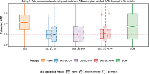
Table D1. Estimated bias, standard error (SE), root mean square error (RMSE), 95% coverage probability, and the average width of a 95% confidence interval, across 3,000 simulations.

Method	Mis-specified Model	Bias	SE	RMSE	Coverage	C.I. Width
Setting 3:
Exist unmeasured confounding and study bias, DID Assumption satisfied, SCM Assumption Not satisfied
RBMI		0.227	0.200	0.303	83.467	0.856
DID-EC-OR	None	−0.000	0.111	0.111	95.133	0.442
	outcome model	−0.003	0.206	0.206	95.067	0.798
DID-EC-IPW	None	0.004	0.217	0.217	95.667	0.907
	ps model	0.003	0.217	0.217	95.867	0.904
DID-EC-AIPW	None	0.004	0.136	0.136	94.867	0.537
	outcome model	0.008	0.216	0.216	94.533	0.845
	ps model	0.003	0.137	0.137	94.567	0.536
SCM		0.154	0.352	0.384	91.400	1.393

Appendix E We present additional simulations, in Figure E1 and Table E1, with a higher percentage of trial controls where the ratio $n_1:n_0$ is approximately $1:1$ instead of $2:1$. All other aspects of the simulations remain the same as in the main simulation, except for setting 3, which is the same as that described in Appendix D, where the study bias is suggested by the observed data. The results are consistent with the main simulation results.

Figure E1. Boxplot of estimated ATEs ${\hat{\tau }}_{\mathit{t}=4}$ across 3,000 simulations, at the last time point. The true ATE ${\tau }_4=2.5$ are represented by the red dashed lines for reference.

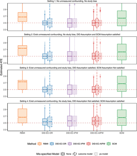
Table E1. Estimated bias, standard error (SE), root mean square error (RMSE), 95% coverage probability, and the average width of a 95% confidence interval, across 3,000 simulations.

Method	Mis-specified Model	Bias	SE	RMSE	Coverage	C.I. Width
Setting 1:
No unmeasured confounding, No study bias
RBMI		0.176	0.204	0.269	89.667	0.883
DID-EC-OR	None	−0.001	0.092	0.092	95.567	0.370
	outcome model	0.000	0.191	0.191	94.667	0.736
DID-EC-IPW	None	−0.002	0.202	0.202	95.633	0.817
	ps model	−0.001	0.202	0.202	95.367	0.814
DID-EC-AIPW	None	−0.001	0.124	0.124	95.233	0.495
	outcome model	0.002	0.200	0.200	94.733	0.790
	ps model	−0.001	0.125	0.125	94.600	0.490
SCM		0.135	0.328	0.354	62.545	0.758
Setting 2:
Exist unmeasured confounding, No study bias, DID Assumption and SCM Assumption satisfied
RBMI		0.199	0.192	0.276	88.200	0.924
DID-EC-OR	None	−0.001	0.110	0.110	94.567	0.430
	outcome model	−0.002	0.193	0.193	95.100	0.762
DID-EC-IPW	None	−0.000	0.207	0.207	95.300	0.826
	ps model	0.000	0.206	0.205	94.867	0.824
DID-EC-AIPW	None	0.003	0.137	0.137	94.967	0.533
	outcome model	0.002	0.211	0.211	94.667	0.806
	ps model	0.003	0.137	0.137	94.167	0.528
SCM		0.127	0.332	0.356	63.306	0.769
Setting 3:
Exist unmeasured confounding and study bias, DID Assumption satisfied, SCM Assumption Not satisfied
RBMI		0.170	0.184	0.251	92.467	0.923
DID-EC-OR	None	0.001	0.111	0.111	94.500	0.430
	outcome model	−0.001	0.196	0.196	95.000	0.764
DID-EC-IPW	None	−0.001	0.208	0.208	95.167	0.825
	ps model	0.000	0.207	0.207	94.767	0.821
DID-EC-AIPW	None	0.001	0.135	0.135	94.933	0.532
	outcome model	−0.004	0.203	0.203	95.533	0.808
	ps model	0.001	0.135	0.135	94.633	0.529
SCM		0.168	0.335	0.375	59.041	0.754
Setting 4:
Exist unmeasured confounding, No study bias, DID Assumption Not satisfied, SCM Assumption satisfied
RBMI		0.198	0.201	0.282	91.067	0.995
DID-EC-OR	None	0.032	0.140	0.143	94.533	0.551
	outcome model	0.036	0.217	0.220	94.400	0.837
DID-EC-IPW	None	0.055	0.225	0.231	94.933	0.911
	ps model	0.056	0.224	0.231	95.000	0.906
DID-EC-AIPW	None	0.054	0.171	0.179	93.033	0.652
	outcome model	0.056	0.230	0.237	94.033	0.890
	ps model	0.055	0.167	0.175	92.900	0.644
SCM		0.158	0.347	0.381	60.860	0.781

References

- Abadie, A. 2005. Semiparametric difference-in-differences estimators. The Review of Economic Studies 72 (1):1–19. doi:10.1111/0034-6527.00321.
- Abadie, A. 2021. Using synthetic controls: Feasibility, data requirements, and methodological aspects. Journal of Economic Literature 59 (2):391–425. doi:10.1257/jel.20191450.
- Abadie, A., A. Diamond, and J. Hainmueller. 2010. Synthetic control methods for comparative case studies: Estimating the effect of california’s tobacco control program. Journal of the American Statistical Association 105 (490):493–505. doi:10.1198/jasa.2009.ap08746.
- Abadie, A., A. Diamond, and J. Hainmueller. 2015. Comparative politics and the synthetic control method. American Journal of Political Science 59 (2):495–510. doi:10.1111/ajps.12116.
- Abadie, A., and J. L’Hour. 2021. A penalized synthetic control estimator for disaggregated data. Journal of the American Statistical Association 116 (536):1817–1834. doi:10.1080/01621459.2021.1971535.
- Bang, H., and J. M. Robins. 2005. Doubly robust estimation in missing data and causal inference models. Biometrics Bulletin 61 (4):962–973. doi:10.1111/j.1541-0420.2005.00377.x.
- Bareinboim, E., and J. Pearl. 2016. Causal inference and the data-fusion problem. Proceedings of the National Academy of Sciences 113 (27):7345–7352. doi:10.1073/pnas.1510507113.
- Berry, S. M., B. P. Carlin, J. J. Lee, and P. Muller. 2010. Bayesian adaptive methods for clinical trials. CRC press.
- Bertini, E., E. Dessaud, E. Mercuri, F. Muntoni, J. Kirschner, C. Reid, A. Lusakowska, G. P. Comi, J.-M. Cuisset, J.-L. Abitbol, et al. 2017. Safety and efficacy of olesoxime in patients with type 2 or non-ambulatory type 3 spinal muscular atrophy: A randomised, double-blind, placebo-controlled phase 2 trial. The Lancet Neurology 16(7):513–522. doi:10.1016/S1474-4422(17)30085-6.
- Buchanan, A. L., M. G. Hudgens, S. R. Cole, K. R. Mollan, P. E. Sax, E. S. Daar, A. A. Adimora, J. J. Eron, and M. J. Mugavero. 2018. Generalizing evidence from randomized trials using inverse probability of sampling weights. Journal of the Royal Statistical Society Series A: Statistics in Society Series A (Statistics in Society) 181 (4):1193–1209. doi:10.1111/rssa.12357.
- Burger, H. U., C. Gerlinger, C. Harbron, A. Koch, M. Posch, J. Rochon, and A. Schiel. 2021. The use of external controls: To what extent can it currently be recommended? Pharmaceutical Statistics 20 (6):1002–1016. doi:10.1002/pst.2120.
- Campbell, D. T. 1957. Factors relevant to the validity of experiments in social settings. Psychological Bulletin 54 (4):297. doi:10.1037/h0040950.
- Carpenter, J. R., J. H. Roger, and M. G. Kenward. 2013. Analysis of longitudinal trials with protocol deviation: A framework for relevant, accessible assumptions, and inference via multiple imputation. Journal of Biopharmaceutical Statistics 23 (6):1352–1371. doi:10.1080/10543406.2013.834911.
- Cole, S. R., and E. A. Stuart. 2010. Generalizing evidence from randomized clinical trials to target populations: The actg 320 trial. American Journal of Epidemiology 172 (1):107–115. doi:10.1093/aje/kwq084.
- Dahabreh, I. J., and M. A. Hernán. 2019. Extending inferences from a randomized trial to a target population. European Journal of Epidemiology 34 (8):719–722. doi:10.1007/s10654-019-00533-2.
- Day, R. O., and K. M. Williams. 2007. Open-label extension studies: Do they provide meaningful information on the safety of new drugs? Drug Safety 30 (2):93–105. doi:10.2165/00002018-200730020-00001.
- Doudchenko, N., and G. W. Imbens. 2016 Balancing, regression, difference-in-differences and synthetic control methods: A synthesis. Tech. rep., National Bureau of Economic Research.
- FDA. 2023. Considerations for the design and conduct of externally controlled trials for drug and biological products - guidance for industry. https://www.fda.gov/media/164960/download.
- Gower-Page, C., and A. Noci. 2022) RBMI: Reference Based Multiple Imputation. https://CRAN.R-project.org/package=rbmi. R package version 1.2.3.
- Heckman, J. J., H. Ichimura, J. A. Smith, and P. E. Todd. 1998. Characterizing selection bias using experimental data.
- Ho, M., M. van der Laan, H. Lee, J. Chen, K. Lee, Y. Fang, W. He, T. Irony, Q. Jiang, X. Lin, et al. 2021. The current landscape in biostatistics of real-world data and evidence: Causal inference frameworks for study design and analysis. Statistics in Biopharmaceutical Research 15(1):43–56. doi:10.1080/19466315.2021.1883475.
- Imbens, G. W., and D. B. Rubin. 2015. Causal inference in statistics, social, and biomedical sciences. Cambridge University Press.
- Kranker, K., L. Blue, and L. V. Forrow. 2021. Improving effect estimates by limiting the variability in inverse propensity score weights. The American Statistician 75 (3):276–287. doi:10.1080/00031305.2020.1737229.
- Li, F., K. L. Morgan, and A. M. Zaslavsky. 2018. Balancing covariates via propensity score weighting. Journal of the American Statistical Association 113 (521):390–400. doi:10.1080/01621459.2016.1260466.
- Lipsitch, M., E. T. Tchetgen, and T. Cohen. 2010. Negative controls: A tool for detecting confounding and bias in observational studies. Epidemiology (Cambridge, Mass.) 21 (3):383. doi:10.1097/EDE.0b013e3181d61eeb.
- McIver, T., M. El-Khairi, W. Y. Yeung, and H. Pang. 2023. The use of real-world data to support the assessment of the benefit and risk of a medicine to treat spinal muscular atrophy. In Real-world evidence in medical product development, (ed. e. a. W. He). Switzerland: Springer Nature.
- Mercuri, E., N. Deconinck, E. S. Mazzone, A. Nascimento, M. Oskoui, K. Saito, C. Vuillerot, G. Baranello, O. Boespflug-Tanguy, N. Goemans, et al. 2022. Safety and efficacy of once-daily risdiplam in type 2 and non-ambulant type 3 spinal muscular atrophy (sunfish part 2): A phase 3, double-blind, randomised, placebo-controlled trial. The Lancet Neurology 21(1):42–52. doi:10.1016/S1474-4422(21)00367-7.
- Oskoui, M., J. W. Day, N. Deconinck, E. S. Mazzone, A. Nascimento, K. Saito, C. Vuillerot, G. Baranello, N. Goemans, J. Kirschner, et al. 2023. Two-year efficacy and safety of risdiplam in patients with type 2 or non-ambulant type 3 spinal muscular atrophy (sma). Journal of Neurology 270(5):2531–2546. doi:10.1007/s00415-023-11560-1.
- Pearl, J. 2009. Causality. Cambridge university press.
- Pearl, J., and E. Bareinboim. 2011. Transportability of causal and statistical relations: A formal approach. In Twenty-fifth AAAI conference on artificial intelligence.
- Pocock, S. J. 1976. The combination of randomized and historical controls in clinical trials. Journal of Chronic Diseases 29 (3):175–188. doi:10.1016/0021-9681(76)90044-8.
- Rubin, D. B. 1977. Assignment to treatment group on the basis of a covariate. Journal of Educational Statistics 2 (1):1–26. doi:10.3102/10769986002001001.
- Sant’anna, P. H., and J. Zhao. 2020. Doubly robust difference-in-differences estimators. Journal of Econometrics 219 (1):101–122. doi:10.1016/j.jeconom.2020.06.003.
- Stuart, E. A., B. Ackerman, and D. Westreich. 2018. Generalizability of randomized trial results to target populations: Design and analysis possibilities. Research on Social Work Practice 28 (5):532–537. doi:10.1177/1049731517720730.
- Wang, H., Y. Fang, W. He, R. Chen, and S. Chen. 2022. Clinical trials with external control: Beyond propensity score matching. Statistics in Biosciences 14 (2):304–317. doi:10.1007/s12561-022-09341-x.
- Westreich, D., J. K. Edwards, C. R. Lesko, E. Stuart, and S. R. Cole. 2017. Transportability of trial results using inverse odds of sampling weights. American Journal of Epidemiology 186 (8):1010–1014. doi:10.1093/aje/kwx164.
- White, I., R. Joseph, and N. Best. 2020. A causal modelling framework for reference-based imputation and tipping point analysis in clinical trials with quantitative outcome. Journal of Biopharmaceutical Statistics 30 (2):334–350. doi:10.1080/10543406.2019.1684308.
- Yap, T. A., I. Jacobs, E. B. Andre, L. J. Lee, D. Beaupre, and L. Azoulay. 2021. Application of real-world data to external control groups in oncology clinical trial drug development. Frontiers in Oncology 11. doi:10.3389/fonc.2021.695936.
- Zubizarreta, J. R. 2015. Stable weights that balance covariates for estimation with incomplete outcome data. Journal of the American Statistical Association 110 (511):910–922. doi:10.1080/01621459.2015.1023805.