
 ?Mathematical formulae have been encoded as MathML and are displayed in this HTML version using MathJax in order to improve their display. Uncheck the box to turn MathJax off. This feature requires Javascript. Click on a formula to zoom.
Abstract
In this paper, we study the gradient descent–ascent method for convex–concave saddle-point problems. We derive a new non-asymptotic global convergence rate in terms of distance to the solution set by using the semidefinite programming performance estimation method. The given convergence rate incorporates most parameters of the problem and it is exact for a large class of strongly convex-strongly concave saddle-point problems for one iteration. We also investigate the algorithm without strong convexity and we provide some necessary and sufficient conditions under which the gradient descent–ascent enjoys linear convergence.
1. Introduction
We consider the convex–concave saddle point problem
(1)
(1) where
, and
and
are convex and concave, respectively, for any fixed
and
. We assume that problem (Equation1
(1)
(1) ) has some solution, that is, there exists a saddle point
with
We denote the solution set of problem (Equation1
(1)
(1) ) with
. We call F smooth if for some
, we have
The function F is said to be strongly convex-strongly concave if
for some
. Note that strong convex-strong concavity implies that problem (Equation1
(1)
(1) ) has a unique solution
. We denote the set of smooth strongly convex-strongly concave functions by
.
Problem (Equation1(1)
(1) ) has applications in game theory [Citation4], robust optimization [Citation5], adversarial training [Citation14], and reinforcement learning [Citation30], to name but a few. In addition, various other algorithms have been developed for solving saddle point problems; see e.g. [Citation15,Citation16,Citation18,Citation25,Citation26,Citation28,Citation29].
One of the simplest approaches for handling problem (Equation1(1)
(1) ) introduced in [Citation2, Chapter 6] is the gradient-descent–ascent method, which may be regarded as a generalization of the gradient method for saddle point problems. The gradient descent–ascent method is described in Algorithm 1.
The local and global linear convergence of Algorithm 1 have been investigated in the literature; see [Citation3,Citation13,Citation17,Citation33] and the references therein. As we investigate the global linear convergence rate of Algorithm 1, we mention one known global convergence result, which is derived by using variational inequality techniques. Suppose that . Let the function
given by
. It is shown that, see e.g. [Citation22],
where
and
. Indeed, ϕ is Lipschitz continuous and strongly monotone. By Facchinei and Pang [Citation12, Theorem 12.1.2], for
, we have
(2)
(2) In this study, we revisit Algorithm 1 and improve the convergence rate (Equation2
(2)
(2) ). Indeed, we derive a new convergence rate involving most parameters of problem (Equation1
(1)
(1) ). It is worth noting that if one sets
and
, the new bound dominates the convergence rate (Equation2
(2)
(2) ) for any step length
. Furthermore, by setting
, one can infer that Algorithm 1 has a complexity of
to compute iterates
such that
, which is the known iteration complexity bound in the literature; see e.g. [Citation6,Citation32]. In this study, thanks to the new convergence rate given in Theorem 2.2, the order of complexity of
is obtained when
and
, which is more informative in comparison with the above-mentioned one. Moreover, by providing some example, we show that the given convergence rate is exact for one iteration.
The goal of this work is not to achieve the optimal algorithmic complexity for the class of saddle point problems introduced above. Rather, we have the more modest goal of giving the best possible worst-case complexity analysis of the gradient descent–ascent method (Algorithm 1). It is important to note that there are accelerated and extra gradient descent–ascent methods with better worst-case complexity than Algorithm 1; see e.g. [Citation18,Citation28]. In particular, the accelerated methods may be shown to have a worst-case complexity , which may be compared to the best-known lower complexity bound
for the class of pure first-order algorithms [Citation34].
The paper is organized as follows. First, we present basic definitions and preliminaries used to establish the results. Section 2 is devoted to the study of the linear convergence of Algorithm 1. In Section 3, we study the linear convergence of the gradient descent–ascent method without strong convexity. Indeed, we let and give some necessary and sufficient conditions for the linear convergence. Moreover, we derive a convergence rate under this setting.
Notation 1
The n-dimensional Euclidean space is denoted by . We use
and
to denote the Euclidean inner product and norm, respectively. For a matrix A,
denotes its
th entry, and
represents the transpose of A. We use
and
to denote the largest and the smallest eigenvalue of symmetric matrix A, respectively.
Let . We denote the distance function to X by
and the set-valued mapping
stands for the projection of x on X, i.e.
.
We call a differentiable function L-smooth if
The function
is called μ-strongly convex function if the function
is convex. Clearly, any convex function is 0-strongly convex. We denote the set of real-valued convex functions which are L-smooth and μ-strongly convex by
.
Let be a finite index set and let
. A set
is called
-interpolable if there exists
with
The next theorem gives necessary and sufficient conditions for
-interpolability.
Theorem 1.1
[Citation27, Theorem 4]
Let and
and let
be a finite index set. The set
is
-interpolable if and only if for any
, we have
(3)
(3)
It is worth mentioning that, under the assumptions of Theorem 1.1, the set is interpolable with an L-smooth μ-strongly concave function if and only if for any
, we have
(4)
(4)
2. The gradient descent–ascent method
In this section, we study the convergence rate of gradient descent–ascent method when with
. Indeed, we investigate the worst-case behaviour of one step of Algorithm 1 in terms of distance to the unique saddle point
for one iterate. Let
be generated by the algorithm using the starting point
. The worst-cast convergence rate is in essence an optimization problem. Indeed, the worst-cast convergence rate of Algorithm 1 is given by the solution of the following abstract optimization problem:
(5)
(5) In problem (Equation5
(5)
(5) ),
are decision variables and
are fixed parameters. At first glace, problem (Equation5
(5)
(5) ) seems completely intractable, but its solution may in fact be approximated using a suitable semidefinite programming (SDP) problem, as shown below. This type of approximation is an example of the so-called SDP performance estimation method, that was introduced by Drori and Teboulle [Citation10].
Suppose that
where indices
refers to the starting point, the point generated by Algorithm 1 and the saddle point of the problem, respectively. Note that due to the the necessary and sufficient conditions for convex–concave saddle point problems, we have
By using Theorem 1.1, problem (Equation5
(5)
(5) ) may be relaxed as a finite dimensional optimization problem,
(6)
(6) In problem (Equation6
(6)
(6) ),
and
are decision variables. We may assume that
and
as Algorithm 1 is invariant under translation. By elimination, problem (Equation6
(6)
(6) ) may be reformulated as follows,
(7)
(7) To approximate the solution of problem (Equation7
(7)
(7) ), we reformulate it as a semidefinite program by using the Gram matrix of the unknown vectors in the problem. Indeed, we form the Gram matrices X and Y as follows,
This results in an SDP problem, as long as we view the value
, that appears in the denominator of the objective of problem (Equation7
(7)
(7) ), as a fixed parameter. For this reason we may indeed view problem (Equation7
(7)
(7) ) as an SDP problem in the positive semidefinite matrix variables X and Y. The interested reader may refer to [Citation27,Citation31] for more details concerning the Gram matrix formulation, and SDP performance estimation in general.
For the convenience of the analysis, we investigate the linear convergence of Algorithm 1 in terms of and
. Before we present the main theorem in this section, we need to present a lemma.
Lemma 2.1
Let ,
and let
. Suppose that the function
given by
Then u is convex on I and
.
Proof.
Consider the function given by
The function v is convex and positive on I. By elementary calculus, one can show that
. So v is increasing on I due to the convexity. As the product of positive monotone convex functions is a convex function, the function
is also convex, which implies the convexity of u. Indeed, u is strictly convex on I. Since strictly convex functions attain their maximum on endpoints of a given interval,
for
. It remains to show that
. This follows from the point that
and the proof is complete.
By the weak duality theorem for SDP, one may demonstrate an upper bound for the optimal value of the SDP problem (Equation7(7)
(7) ), by constructing a feasible solution to its dual problem, i.e. feasible dual multipliers for the constraints of problem (Equation7
(7)
(7) ). This is done in the next theorem. In the proof, the correct value of the dual multipliers are simply given, and their correctness is verified. The correct values were obtained by solving the SDP problem (Equation7
(7)
(7) ) repeatedly for different numerical values of the parameters, and noting the (numerical) optimal dual multiplier values. Based on these values, it was possible to deduce the analytical expressions for the multipliers. For this reason, the proof was found in a computer-assisted way, but it does not rely on any numerical calculations. Having said that, the proof involves a long identity, given in full in Appendix 2 to this paper, that is so long that it could only be obtained in a computer-assisted way.
Theorem 2.2
Let . Suppose that
and
. If
, then Algorithm 1 generates
such that
(8)
(8) where
Proof.
As mentioned earlier, we may assume without loss of generality that and
. By assumption,
and
for any fixed x, y. Without loss of generality, we may also assume that
, by replacing F by
. This follows from the observation that Algorithm 1 generates the same point
for the problem
with the step length
. Moreover, one has
if and only if
. Now let
and define (the multipliers):
It is readily verified that
, but since this calculation is somewhat tedious we present it in Appendix 1. Moreover, Lemma 2.1 implies that
.
The idea of the proof is now as follows: we first establish that, for any feasible solution of the SDP problem (Equation7(7)
(7) ), it holds that
(9)
(9) We do this by establishing an algebraic identity for the left-hand side of the inequality (Equation9
(9)
(9) ). The first and last terms of this identity (shown in full in Appendix 2 to this paper) are as follows:
Note that the first term on the right-hand side is indeed non-positive, since
, and the expression in brackets is non-negative at any feasible solution of the SDP problem (Equation7
(7)
(7) ), since it corresponds to one of the constraints in (Equation7
(7)
(7) ). The last term is non-positive as well, since it is the product of a non-positive multiplier with a squared expression. The remaining terms in the identity are similarly non-positive (see Appendix 2), proving the inequality (Equation9
(9)
(9) ). All that remains is to recognize that, in (Equation9
(9)
(9) ),
corresponds to
, so that
corresponds to
, etc. This yields the statement of the theorem, after rescaling to remove the assumption
.
One may wonder how we obtained the (analytical) expression for α in Theorem 2.2. Consider the optimization problem
(10)
(10) where
. It is known that the quadratic function
with
and
attains the worst-case convergence rate for the gradient method; see e.g. [Citation9]. We guessed that this property may hold for problem (Equation1
(1)
(1) ) and we investigated the bilinear saddle point problem
(11)
(11) where
,
and
are fixed parameters and we derived the worst case convergence of Algorithm 1 with respect to this problem. Our numerical experiments showed that the derived convergence rate is the same as the optimal value of the semidefinite programming problem corresponding to problem (Equation7
(7)
(7) ). Moreover, as a by-product, we exhibit that the convergence rate (Equation8
(8)
(8) ) is exact for one iteration by using problem (Equation11
(11)
(11) ); see Proposition 2.4.
Theorem 2.2 provides some new information concerning Algorithm 1. Firstly, Theorem 2.2 improves the known convergence factor in the literature; see our discussion in Introduction. In addition, it investigates the convergence rate for a step length in a larger interval. Secondly, it does not assume the second order continuous differentiability of F, which is commonly used for deriving a local convergence rate; see [Citation17,Citation20,Citation33]. Finally, the given convergence rate incorporates three parameter ,
and
, which is more informative in comparison with the results in the literature mostly given in terms of
and
; see [Citation21,Citation33,Citation34] and references therein. Even though if one considers
and
, convergence rate (Equation8
(8)
(8) ) dominates (Equation2
(2)
(2) ). This follows from that for
, one has
where the first inequality results from
. In addition, in this case, the step length can take value in a larger interval as
. Moreover, Conjecture 2.6 discusses the convergence rate in terms of
.
The next proposition gives the optimal step length with respect to the worst case convergence rate.
Proposition 2.3
Let . If
and
, then the optimal step length for Algorithm 1 with respect to the bound (Equation8
(8)
(8) ) is
(12)
(12) Moreover, the convergence rate with respect to
is
(13)
(13)
Proof.
Let given by
By Lemma 2.1, α is a strictly convex function on its domain. By doing some algebra, one can verify that
, which implies that
is the minimum.
If , problem (Equation1
(1)
(1) ) reduces to a separable optimization problem. Indeed, the variables x and y are independent. Under this assumption, the optimal step length given by Proposition 2.3 is
, which is the well-known optimal step length for the optimization problem
where
; see [Citation24, Theorem 2.1.15]. Moreover, the convergence rate corresponding to
is
. By some algebra, one can show that under the assumptions of Proposition (2.3), Algorithm 1 has a complexity of
. Note that the lower iteration complexity bound for first-order methods with
and
is
; see [Citation34].
As mentioned earlier, we calculated the convergence rate by using problem (Equation11(11)
(11) ). The next proposition states that the bound (Equation8
(8)
(8) ) is tight for some class of bilinear saddle point problems.
Proposition 2.4
Let . Suppose that
and
. If
, then convergence rate (Equation8
(8)
(8) ) is exact for one iteration.
Proof.
To establish the proposition, it suffices to introduce a problem for which Algorithm 1 generates with respect to the initial point
such that
where α is the convergence rate factor given in Theorem 2.2. Consider problem (Equation11
(11)
(11) ). Due to the symmetry of Algorithm 1 and the class of problems, we may assume
. Moreover, without loss of generality, we can take
; see our discussion in the proof of Theorem 2.2. Suppose
,
and
. One can verify that Algorithm 1 with the initial point
generates
with the desired equality.
One may wonder why we stress on one iteration in Proposition 2.4. Based on our numerical results if , under the setting of Theorem 2.2, we observed that
for some
. The reason may be related to the fact that the vector field
is not conservative.
It may be of interest whether inequality (Equation8(8)
(8) ) may hold without strong convexity. By removing strong convexity, the solution set may not be singleton. Hence, we investigate distance to the solution set, that is, if there exists
with
The next proposition says in general the answer is negative. Indeed, it gives an example with
and a unique saddle point for which
for some
, no matter how close
is to the unique saddle point and which positive step length t is taken. In the next proposition, we may assume without loss of generality
and make an example analogous to that given in Proposition 2.4.
Proposition 2.5
Let be given. Then there exist
and a function
with the unique saddle point
and
such that, for
generated by Algorithm 1, we have
and
.
Proof.
As discussed before, we may assume . Consider the bilinear saddle point problem,
It is clear that
, and the unique saddle point is
. Suppose that
where
. One can verify Algorithm 1 generates
with
where
. By Proposition 2.3, one can infer that
.
Note that r can take any positive value in Proposition 2.5. By Proposition 2.4, one can infer that the convergence rate factor for bilinear saddle point problems may not be improved for one iteration since the given example is a bilinear saddle point problem. Furthermore, the given convergence rate factor is tight whether . As discussed in [Citation28], the function
shares the same smoothness constants with respect to x and y, that is,
and
are Lipschitz continuous with the same modulus
. However, the gradient methods are not invariant under scaling; see [Citation8, Chapter 9]. Hence, we may lose the generality of our discussion by assuming this condition.
Based on our numerical results and analysis of problem (Equation11(11)
(11) ), we conjecture the following (exact) convergence rate of Algorithm 1 in terms of
. Due to the symmetry of Algorithm 1, we may assume that
. Moreover, Proposition 2.4 implies that bound (Equation8
(8)
(8) ) is tight when
. Hence, we need only consider
.
Conjecture 2.6
Let . Suppose that
,
and
Then, one of the following scenarios holds.
Assume that
and
If
If
Assume that
If
If
Although we have extensive numerical evidence supporting Conjecture 2.6, we have been unable to prove either part (a) or part (b). To be more precise, we have verified numerically that the optimal value of the SDP problems (Equation7(7)
(7) ) and (Equation11
(11)
(11) ) corresponds to the expressions in Conjecture 2.6 for many different numerical values of the parameters
,
,
,
, and
, but we could not manage to derive analytical expressions for the dual multipliers of SDP problem (Equation7
(7)
(7) ) for proving the conjecture.
2.1. Numerical illustration
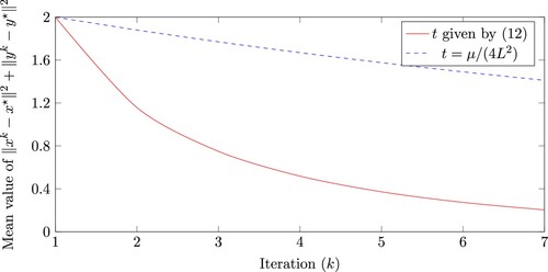
In this section we provide randomly generated examples to compare the optimal step length (Equation12(12)
(12) ) given in this paper to the known step length
for the bilinear problem
where
and
are symmetric positive definite matrices. Moreover, the instances are constructed such that the spectra of
and
are contained in the interval
. For this class of instances, one has
and
. The matrix
has entries chosen uniformly at random from
, and subsequently we set
. By construction, the solution (saddle point) is
. The starting points
and
are randomly drawn unit vectors so that the initial condition
is satisfied.
In Figure we show average values (over 100 randomly generated instances) for the convergence indicator after k iterations, for the two step lengths.Footnote1 Note that our new step length (Equation12
(12)
(12) ) gives a clear improvement over the known step length
.
Figure 1. Mean values of for 100 randomly generated instances for each iteration k using the two different step lengths t.
3. Linear convergence without strong convexity
In this section, we study the linear convergence of Algorithm 1 without assuming strong convexity. Indeed, we suppose that and we propose some necessary and sufficient conditions for the linear convergence. This subject has received some attention in recent years and some sufficient conditions have been proposed in [Citation11,Citation33] under which Algorithm 1 enjoys local linear convergence rate or it is linearly convergent for bilinear saddle point problems. This topic has been investigated extensively in the context of optimization. The interested reader can refer to [Citation1,Citation7,Citation19,Citation23] and references therein. In this study, we extend the quadratic gradient growth property introduced in [Citation19] for saddle point problems.
Recall that we denote the non-empty solution set of problem (Equation1(1)
(1) ) by
. As we do not assume the strong convexity (concavity),
may not be singleton. Note that
is a closed convex set under our assumptions. Recall that
denotes the projection of
onto
.
Definition 3.1
Let . A function F has a quadratic gradient growth if for any
and
,
(14)
(14) where
.
Note that if we set in (Equation14
(14)
(14) ), we have
Hence,
-smoothness implies that
. Consequently, due to the symmetry, we have
. The next proposition states that the quadratic gradient growth condition is weaker than the strong convexity-strong concavity. Indeed, the strong convexity–strong concavity implies the quadratic gradient growth property.
Proposition 3.2
Let . If
, then F has a quadratic gradient growth with
.
Proof.
Under the assumptions, problem (Equation1(1)
(1) ) has a unique solution
and
and
. Let
and
. Suppose that
. By Theorem 1.1, we have
Hence,
and the proof is complete.
Note that the converse of Proposition 3.2 does not hold necessarily. Consider the following saddle point problem
(15)
(15) where
It is seen that F is not strongly convex-strongly concave and the solution set of problem (Equation15
(15)
(15) ) is
. By doing some algebra, one can check that F has a quadratic gradient growth with
while it is not strongly convex with respect to the first component. For the case that
is neither strongly convex nor is
strongly concave, one may consider uncoupled problem
.
In what follows, by using performance estimation, we establish that Algorithm 1 enjoys the linear convergence whether has a quadratic gradient growth. Without loss of generality, we may assume that
. To establish the linear convergence, it suffices to show that
for some
. Similarly to Section 2, we formulate the following optimization problem
(16)
(16) Note that in the formulation (Equation16
(16)
(16) ), we only use a subset of constraints for the performance estimation. In the next theorem, we prove the linear convergence of Algorithm 1 when F has a quadratic gradient growth.
Theorem 3.3
Let and
. Assume that F has a quadratic gradient growth with
. If
, then Algorithm 1 generates
such that
(17)
(17) where
Proof.
The argument is similar to that of Theorem 2.2. It is seen that for any step length t in the given interval, . We may assume without loss of generality
. By the assumptions,
and
for any fixed x, y. Suppose that
One may readily verify that
. By doing some algebra, one can show that
where the multipliers
are given as follows
One can show by some algebra that
. Hence, for any feasible solution of problem (Equation16
(16)
(16) ), we have
and the proof is complete.
We obtained the linear convergence by using quadratic gradient growth in Theorem 3.3. The next theorem states that quadratic gradient growth property is also a sufficient condition for the linear convergence.
Theorem 3.4
If Algorithm 1 is linearly convergent for any initial point, then F has a quadratic gradient growth for some .
Proof.
Let and
be generated by Algorithm 1. Suppose that
. As Algorithm 1 is linearly convergent, there exist
with
(18)
(18) By setting
and
in inequality (Equation18
(18)
(18) ), we get
which implies that
for
and the proof is complete.
4. Concluding remarks
In this study, we provided a new convergence rate for the gradient descent–ascent method for saddle point problems. Furthermore, we gave some necessary and sufficient conditions for the linear convergence without strong convexity. We employed performance estimation method for proving the results. For future work, it would be interesting to consider the case where the variables x and y in the saddle point problem are constrained to lie in given, compact convex sets, since many saddle point problems fall in this category. In this case, one could use the performance estimation framework to analyse other methods, e.g. proximal type algorithms.
Disclosure statement
No potential conflict of interest was reported by the author(s).
Additional information
Funding
Notes on contributors
Moslem Zamani
Moslem Zamani obtained his PhD degree from the University of Avignon and the University of Tehran. He worked as a postdoctoral researcher at Tilburg University. He is currently a researcher at UCLouvain. His main research interests include non-linear optimization and machine learning algorithms.
Hadi Abbaszadehpeivasti
Hadi Abbaszadehpeivasti earned his bachelor's degree in applied mathematics from the University of Zanjan and subsequently obtained master's degrees in industrial engineering from both Sharif University of Technology and Sabancı University. He is currently a PhD. student at Tilburg University, focusing on the complexity of first-order methods. His primary research interests include mathematical optimization and machine learning algorithms.
Etienne de Klerk
Etienne de Klerk obtained his PhD degree from the Delft University of Technology in The Netherlands in 1997. From January 1998 to September 2003, he held assistant professorships at the Delft University of Technology, and from September 2003 to September 2005 an associate professorship at the University of Waterloo, Canada, in the Department of Combinatorics & Optimization. In September 2004 he was appointed at Tilburg University, The Netherlands, first as an associate professor, and then as full professor (from June 2009). From August 29th, 2012, until August 31st, 2013, he was also appointed as full professor in the Division of Mathematics of the School of Physical and Mathematical Sciences at the Nanyang Technological University in Singapore. From September 1st, 2015 to August 31st 2019, he also held a part-time full professorship at the Delft University of Technology. Dr. De Klerk's main research interest is mathematical optimization, and, in particular, semidefinite programming.
Notes
1 The 100 random instances and starting points that we generated to produce Figure may be found on GitHub; see: https://github.com/molsemzamani/Bilinear-Minimax.
References
- H. Abbaszadehpeivasti, E. de Klerk, and M. Zamani, Conditions for linear convergence of the gradient method for non-convex optimization, Optim. Lett. 17 (2023), pp. 1105–1125.
- K.J. Arrow, H. Azawa, L. Hurwicz, H. Uzawa, H.B. Chenery, S.M. Johnson, and S. Karlin, Studies in Linear and Non-linear Programming, Vol. 2, Stanford University Press, California, 1958.
- W. Azizian, I. Mitliagkas, S. Lacoste-Julien and G. Gidel, A tight and unified analysis of gradient-based methods for a whole spectrum of differentiable games, in International Conference on Artificial Intelligence and Statistics, PMLR, 2020, pp. 2863–2873.
- T. Başar and G.J. Olsder, Dynamic Noncooperative Game Theory, SIAM, Philadelphia, PA, 1998.
- A. Ben-Tal, L. El Ghaoui, and A. Nemirovski, Robust Optimization, Vol. 28, Princeton University Press, Princeton, 2009.
- A. Beznosikov, B. Polyak, E. Gorbunov, D. Kovalev, and A. Gasnikov, Smooth monotone stochastic variational inequalities and saddle point problems – survey, preprint (2022). Available at arXiv:2208.13592.
- J. Bolte, T.P. Nguyen, J. Peypouquet, and B.W. Suter, From error bounds to the complexity of first-order descent methods for convex functions, Math. Program. 165 (2017), pp. 471–507.
- S. Boyd and L. Vandenberghe, Convex optimization, Cambridge University Press, Cambridge, 2004.
- E. De Klerk, F. Glineur, and A.B. Taylor, On the worst-case complexity of the gradient method with exact line search for smooth strongly convex functions, Optim. Lett. 11 (2017), pp. 1185–1199.
- Y. Drori and M. Teboulle, Performance of first-order methods for smooth convex minimization: A novel approach, Math. Program. 145 (2014), pp. 451–482.
- S.S. Du and W. Hu, Linear convergence of the primal-dual gradient method for convex–concave saddle point problems without strong convexity, in The 22nd International Conference on Artificial Intelligence and Statistics, PMLR, 2019, pp. 196–205.
- F. Facchinei and J.S. Pang, Finite-Dimensional Variational Inequalities and Complementarity Problems, Springer, New York, 2003.
- A. Fallah, A. Ozdaglar and S. Pattathil, An optimal multistage stochastic gradient method for minimax problems, in 2020 59th IEEE Conference on Decision and Control (CDC), IEEE, 2020, pp. 3573–3579.
- I. Goodfellow, J. Pouget-Abadie, M. Mirza, B. Xu, D. Warde-Farley, S. Ozair, A. Courville, and Y. Bengio, Generative adversarial nets, Adv. Neural. Inf. Process. Syst. 27 (2014), pp. 1–9.
- E.Y. Hamedani and N.S. Aybat, A primal-dual algorithm with line search for general convex–concave saddle point problems, SIAM. J. Optim. 31 (2021), pp. 1299–1329.
- R. Jiang and A. Mokhtari, Generalized optimistic methods for convex–concave saddle point problems, preprint (2022). Available at arXiv:2202.09674.
- T. Liang and J. Stokes, Interaction matters: A note on non-asymptotic local convergence of generative adversarial networks, in The 22nd International Conference on Artificial Intelligence and Statistics, PMLR, 2019, pp. 907–915.
- T. Lin, C. Jin and M.I. Jordan, Near-optimal algorithms for minimax optimization, in Conference on Learning Theory, PMLR, 2020, pp. 2738–2779.
- Z.Q. Luo and P. Tseng, Error bounds and convergence analysis of feasible descent methods: A general approach, Ann. Oper. Res. 46 (1993), pp. 157–178.
- L. Mescheder, S. Nowozin, and A. Geiger, The numerics of gans, Adv. Neural. Inf. Process. Syst. 30 (2017), pp. 1–11.
- A. Mokhtari, A. Ozdaglar and S. Pattathil, A unified analysis of extra-gradient and optimistic gradient methods for saddle point problems: Proximal point approach, in International Conference on Artificial Intelligence and Statistics, PMLR, 2020, pp. 1497–1507.
- A. Mokhtari, A.E. Ozdaglar, and S. Pattathil, Convergence rate of O(1/k) for optimistic gradient and extragradient methods in smooth convex–concave saddle point problems, SIAM. J. Optim. 30 (2020), pp. 3230–3251.
- I. Necoara, Y. Nesterov, and F. Glineur, Linear convergence of first order methods for non-strongly convex optimization, Math. Program. 175 (2019), pp. 69–107.
- Y. Nesterov, Lectures on Convex Optimization, Vol. 137, Springer, Berlin, 2018.
- J. Nie, Z. Yang, and G. Zhou, The saddle point problem of polynomials, Found. Comput. Math. 22 (2022), pp. 1133–1169.
- J.W. Simpson-Porco, B.K. Poolla, N. Monshizadeh, and F. Dörfler, Input–output performance of linear–quadratic saddle-point algorithms with application to distributed resource allocation problems, IEEE. Trans. Automat. Contr. 65 (2019), pp. 2032–2045.
- A.B. Taylor, J.M. Hendrickx, and F. Glineur, Smooth strongly convex interpolation and exact worst-case performance of first-order methods, Math. Program. 161 (2017), pp. 307–345.
- Y. Wang and J. Li, Improved algorithms for convex–concave minimax optimization, Adv. Neural. Inf. Process. Syst. 33 (2020), pp. 4800–4810.
- Z. Xu, H. Zhang, Y. Xu, and G. Lan, A unified single-loop alternating gradient projection algorithm for nonconvex–concave and convex–nonconcave minimax problems, Math. Program. 201 (2023), pp. 635–706.
- M. Yang, O. Nachum, B. Dai, L. Li, and D. Schuurmans, Off-policy evaluation via the regularized Lagrangian, Adv. Neural. Inf. Process. Syst. 33 (2020), pp. 6551–6561.
- M. Zamani, H. Abbaszadehpeivasti, and E. de Klerk, The exact worst-case convergence rate of the alternating direction method of multipliers, preprint (2022). Available at arXiv:2206.09865.
- G. Zhang, X. Bao, L. Lessard, and R. Grosse, A unified analysis of first-order methods for smooth games via integral quadratic constraints, J. Mach. Learn. Res. 22 (2021), pp. 1–39.
- G. Zhang, Y. Wang, L. Lessard and R.B. Grosse, Near-optimal local convergence of alternating gradient descent–ascent for minimax optimization, in International Conference on Artificial Intelligence and Statistics, PMLR, 2022, pp. 7659–7679.
- J. Zhang, M. Hong, and S. Zhang, On lower iteration complexity bounds for the convex concave saddle point problems, Math. Program. 194 (2022), pp. 901–935.
Appendices
Appendix 1.
Non-negativity of multipliers in Theorem 2.2
Recall that, in the proof of Theorem 2.2, is defined by
Since t is non-negative, we only need to prove that
is non-negative. We show that the following optimization problem is lower bounded by zero,
where
are decision variables. First we consider the case that
. We have the following optimization problem
(A1)
(A1) The function
is concave in μ, therefore, we just consider
and
.
First we consider the case that . By substituting
in
we have
We argue that the above function is non-negative on the feasible set of problem (EquationA1
(A1)
(A1) ). By a conjugate multiplication of
one has
since
we conclude that
which proves
is non-negative.
Now we consider the case that . By substituting
we have
Now we show that
is non-negative on the given set. Note that, again by conjugate multiplication,
which always is non-negative due to the non-negativity of
.
Now we consider the case that tL−1>0. We have
Here, we need to consider two sub-cases. Firstly, when
, we have
If
, we have
which completes the proof.
To show that is non-negative we follow the same procedure. Recall the definition of
We define
as
Due to
, we only need to show that
is non-negative. To this end, we show that the following optimization problem is lower bounded by zero.
First we consider the case that
. We have
We consider two sub-cases. Firstly,
:
Now assume that
.
Now we consider the case that
.
Note that
is concave with respect to the variable L. Therefore, we should study the boundaries of L. If we set
we have
By conjugate multiplication, we have
By
one can see that
. Setting
:
This completes the proof.
Appendix 2.
Identity used in the proof of Theorem 2.2
The proof of Theorem 2.2 requires the following identity, that may be verified through direct (symbolic) calculation:
where
are given by
Note that
, as required.