Numerical simulation of differential-algebraic equations with embedded global optimization criteria

Abstract

We are considering differential-algebraic equations with embedded optimization criteria (DAEOs), in which the embedded optimization problem is solved by global optimization. This leads to differential inclusions for cases in which there are multiple global optimizers at the same time. Jump events from one global optimum to another result in nonsmooth DAEs and reduce the order of convergence of the numerical integrator to first-order. Implementation of event detection and location as introduced in this work preserves the higher-order convergence behaviour of the integrator. This allows the computation of discrete tangent and adjoint sensitivities for optimal control problems.

Keywords:

• Higher-order numerical integrator
• global optimization
• nonsmooth dynamic system

2020 MATHEMATICS SUBJECT CLASSIFICATIONS:

• 90C26
• 49J52
• 65L80

1. Introduction

Solving dynamic models that are described by underdetermined systems of differential-algebraic equations (DAEs) when there are more algebraic states than algebraic equations often requires the embedding of an optimization criterion to find a unique solution. These models are called DAEs with embedded optimization criteria (DAEOs).

Prime application for DAEOs can be found in process system engineering. Separation processes with thermodynamic equilibrium between phases are often modelled with DAEOs. The DAE describes the dynamic behaviour, and a nonlinear programme represents the phase equilibrium as being at the minimum of the Gibbs free energy [1,9,29].

For simulation [26,27] and optimization [5,16,28] of DAEOs, the nonlinear programmes are often substituted with first-order optimality conditions, e.g. Karush–Kuhn–Tucker (KKT) conditions. For nonconvex nonlinear programmes, the solution point might only be locally optimal. The local approach only guarantees exact solution for convex nonlinear programmes. Furthermore, substitution of the optimization problem by the KKT conditions yields a nonsmooth DAE due to switching events, i.e. changes of the active set. This kind of problem is solved either with a simultaneous or with a sequential approach [4]. The simultaneous approach involves solving a single large-scale NLP. In contrast, the sequential approach requires interaction of the numerical integrator and the numerical optimizer.

In this paper, we propose a method to solve DAEOs with deterministic global optimization (DGO) methods instead of substituting the optimization problem with first-order optimality conditions. The proposed method guarantees that the solution point of the optimization problem is a global optimum. Embedding a global optimization problem requires the consideration of differential inclusions as a generalization of differential equations for the cases where several global optimizers exist. Among other things, this is also the case when the global optimizer jumps. A jump of the global optimizer is referred to as an event, which can occur due to the nature of dynamic systems. In the presence of an event, the resulting DAE system becomes nonsmooth. Using the local optimum of the previous time step even if the time period covers an event amounts to a type of discontinuity locking [25]. Unfortunately, the convergence order of the integrator is reduced to first-order without explicit treatment of event locations. To achieve second-order convergence across jumps of the global optimum it is necessary to implement an adaptive time stepping or event location procedure. We will describe how to detect and locate events.

An alternative approach for obtaining a higher convergence for the integrator is presented in [14]. They utilize a generalization of algorithmic differentiation (AD) to treat nonsmooth right hand sides of ordinary differential equations (ODEs). Further information on the theory of AD can be found in [11,24] and for information on nonsmooth AD, see [12,17].

The paper is organized as follows: In Section 2, we describe the mathematical formulation of the type of problem we are considering in this paper. This includes the description of the DAEO and assumptions on the DAEO and on the events. Section 3 gives an overview of interval computations and deterministic global optimization. Based on [6], we show how to obtain those boxes produced during a divide-and-conquer algorithm that potentially contain a local minimum of a nonconvex objective function. The numerical simulation of the DAEO is described in Section 4, including a description of the event detection and event location processes. In Section 5 the presented methods are applied to two example functions. For the first example, we derive an analytical solution to examine the convergence behaviour of the simulation with and without explicit treatment of the events. Section 6 summarizes the results and gives an outlook on future work.

2. Theoretical background

We consider the initial value problem for a differential inclusion with an embedded global optimization problem (1a) $\begin{array}{rl}x(t_0)& =x_0,\end{array}$(1a) (1b) $\begin{array}{rl}{x}^{\prime }(t)& =f(x(t),y(x(t))),\end{array}$(1b) (1c) $\begin{array}{rl}y(x(t))& \in {\arg \min }_{y}h(x(t),y)\mathrm{\forall }t\in (t_0,T),\end{array}$(1c) where $f:{\mathbb{R}}^{n_x}\times {\mathbb{R}}^{n_y}\to {\mathbb{R}}^{n_x}$ is the differential part of the system and $h:{\mathbb{R}}^{n_x}\times {\mathbb{R}}^{n_y}\to \mathbb{R}$ is the objective function. We use the notation $x^{\prime }=\mathrm{\partial }x/\mathrm{\partial t}$ for the derivative with respect to time, ${\mathrm{d}}_t=\mathrm{d}/\mathrm{d}t$ for the total derivative with respect to time, ${\mathrm{\partial }}_x=\mathrm{\partial }/\mathrm{\partial }x$ for the (partial) derivative and ${\mathrm{d}}_x=\mathrm{d}/\mathrm{d}x$ for the total derivative with respect to x where it is crucial to distinguish from the partial derivative in the context of implicit differentiation. Second partial derivatives are denoted by ${\mathrm{\partial }}_{\mathrm{yx}}^2={\mathrm{\partial }}^2/\mathrm{\partial }y\mathrm{\partial x}$. For simplicity of notation, we restrict the discussion throughout to the case $n_y=1$. However, it is possible to extend the results to general $n_y$ with some technical effort.

The problem in (1) is a differential inclusion instead of a differential equation problem because the optimum of the embedded optimization problem is not necessarily unique. We consider the case where the solution set consists of a finite set of isolated strict local optima that are also potential global optima (2) ${\arg \min }_{y}h(x,y)=\{y^1(x),\dots ,y^S(x)\},$(2) with $h(x,y^i(x))=h(x,y^j(x))$ for all $i,j\in \{1,\dots ,S\}$ and $h(x,y^i(x))<h(x,z)$ for all $i\in \{1,\dots ,S\}$, $z\in {\mathbb{R}}^{n_y}\setminus {\arg \min }_{y}h(x,y(x))$.

Assumption 2.1

The functions f and h are twice Lipschitz continuously differentiable with respect to $(x,y)$.

Definition 2.1

We use the notation $\mathbf{A}\succ 0$ for symmetric positive definite matrix $\mathbf{A}\in {\mathbb{R}}^{n\times n}$: $\mathbf{A}\succ 0\iff x^{\mathrm{\top }}\mathbf{A}x>0\mathrm{\forall }x\in {\mathbb{R}}^n\mathrm{\setminus }0.$The smallest eigenvalue of $\mathbf{A}$ is equal to $\{inf{x}^{\mathrm{\top }}\mathbf{A}x\mid x\in {\mathbb{R}}^n\mathrm{with}\Vert x{\Vert }_2=1\}$.

Furthermore, we write a matrix $\mathbf{A}$ with eigenvalues larger than or equal to δ as follows: $\mathbf{A}⪰\delta \iff \mathbf{A}-\delta \mathbf{I}⪰0,$with identity matrix $\mathbf{I}\in {\mathbb{R}}^{n\times n}$.

For each strict local optimum we have necessary and sufficient local optimality conditions (3a) $\begin{array}{rl}0& ={\mathrm{\partial }}_{y}h(x,y),\end{array}$(3a) (3b) $\begin{array}{rl}0& \prec {\mathrm{\partial }}_{\mathrm{yy}}^{2}h(x,y).\end{array}$(3b) The gradient with regard to y is zero and the Hessian is positive definite.

Assumption 2.2

The initial value problem is posed in such a way that the necessary and sufficient local optimality conditions in (3) hold for $(x(t),y^i(x(t))$ for all $i\in \{1,\dots ,S\},t\in [t_0,T]$.

In order to turn the differential inclusion into a discontinuous differential equation with a unique solution, we consider the case where the solution set has size larger than one only for a set of times that has measure zero. We make the even stronger assumptions that the set of times where the solution set is larger than one is finite in order to make handling these events numerically feasible.

Assumption 2.3

There exists a finite set of events $0<{\tau }^1<\cdots <{\tau }^K<T$ with $|{\arg \min }_{y}h(x({\tau }^j),y)|=2,$for all $j\in \{1,\dots K\}$ and we have $|{\arg \min }_{y}h(x(t),y)|=1,$for all $t\in [t_0,T]$ with $t\ne {\tau }^j$ for some $j\in \{1,\dots K\}$.

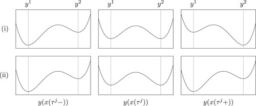
With the previous assumption we can have two cases for each ${\tau }^j$.

1. The switch from one global optimizer to another: ${\arg \min }_{y}h(x({\tau }^j),y))=\{y^1(x({\tau }^j)),y^2(x({\tau }^j))\},$and $\begin{array}{rl}\underset{t\to {\tau }^j-}{lim}{\arg \min }_{y}h(x(t),y)& =\{y^1(x({\tau }^j))\},\\ \underset{t\to {\tau }^j+}{lim}{\arg \min }_{y}h(x(t),y)& =\{y^2(x({\tau }^j))\}.\end{array}$See Figure 1(top) for a visualization.

2. The touching of a second local optimum: ${\arg \min }_{y}h(x({\tau }^j),y)=\{y^1(x({\tau }^j)),y^2(x({\tau }^j))\},$and $\begin{array}{rl}\underset{t\to {\tau }^j-}{lim}{\arg \min }_{y}h(x(t),y)& =\{y^1(x({\tau }^j))\},\\ \underset{t\to {\tau }^j+}{lim}{\arg \min }_{y}h(x(t),y)& =\{y^1(x({\tau }^j))\}.\end{array}$See Figure 1(bottom) for a visualization.

The second case is not relevant for the solution of the differential equation because it occurs on a set of measure zero. We make a transversality assumption that precludes the second case. First, we define the condition of the touching two local optima $y^1(x(t))$ and $y^2(x(t))$ as the root of the event function $H(x(t),y^1(x(t)),y^2(x(t)))$ (4) $0=h(x,y^1)-h(x,y^2)=H(x,y^1,y^2).$(4)

Figure 1. Cases resulting from Assumption 2.3.

Assumption 2.4

All events are transversal, ${\mathrm{d}}_{t}H(x({\tau }^j),y^1(x({\tau }^j)),y^2(x({\tau }^j)))>0,j\in \{1,\dots ,K\}.$With $y^1(x(t))$ and $y^2(x(t))$ fulfilling the first-order optimality, i.e. (3a(3a) $\begin{array}{rl}0& ={\mathrm{\partial }}_{y}h(x,y),\end{array}$(3a) ), and assuming that $y(x({\tau }^j))=y^1(x({\tau }^j-))$ we have $\begin{array}{rl}{\mathrm{\partial }}_{x}H(x({\tau }^j),y^1(x({\tau }^j)),y^2(x({\tau }^j)))f(x({\tau }^j),y^1(x({\tau }^j)))& >0,\\ {\mathrm{\partial }}_{x}H(x({\tau }^j),y^1(x({\tau }^j)),y^2(x({\tau }^j)))f(x({\tau }^j),y^2(x({\tau }^j)))& >0,j\in \{1,\dots ,K\}.\end{array}$

With the above assumptions we can write the original differential inclusion posed in (1) as multiple initial value problems for differential equations for $j=0,\dots ,K+1$: (5a) $\begin{array}{rl}{x}^j({\tau }^j)& =\{\begin{array}{ll}{x}_0& \mathrm{if}j=0\\ x^{j-1}({\tau }^j)& \mathrm{otherwise}\end{array}\end{array}$(5a) (5b) $\begin{array}{rl}(x^j{)}^{\prime }(t)& =f(x^j(t),y^j(x(t)))\end{array}$(5b) (5c) $\begin{array}{rl}\{y^j(x(t))\}& ={\arg \min }_{y}h(x^j(t),y)t\in ({\tau }^j,{\tau }^{j+1}),\end{array}$(5c) where $t^0=t_0$ and $t^{K+1}=T$. The time periods $({\tau }^j,{\tau }^{j+1})$, $j=0,\dots ,K$, will be referred to as phases.

Proposition 2.1

(5) is a DAEO for each phase because $y^j(x(t))$ is a locally unique implicit function of $x(t)$ that is also Lipschitz continuous in $x(t)$.

Proof.

Due to Assumption 2.2, the first-order optimality condition holds for all local optima. By the implicit function theorem and usage of the positive definiteness of the Hessian, we have (6) $\begin{array}{rl}{\mathrm{d}}_x{\mathrm{\partial }}_{y}h(x,y)& ={\mathrm{\partial }}_{\mathrm{yy}}^{2}h(x,y){\mathrm{\partial }}_{x}y(x)+{\mathrm{\partial }}_{\mathrm{yx}}^{2}h(x,y)=0\\ \Rightarrow {\mathrm{\partial }}_{x}y(x)& =-{\mathrm{\partial }}_{\mathrm{yy}}^{2}h(x,y{)}^{-1}{\mathrm{\partial }}_{\mathrm{yx}}^{2}h(x,y).\end{array}$(6)

Because y is only given implicitly, the above problems are really DAEs of index 1.

We get the DAE formulation by imposing the first-order optimality condition: (7a) $\begin{array}{rl}{x}^j({\tau }^j)& =\{\begin{array}{ll}{x}_0& \mathrm{if}j=0\\ x^{j-1}({\tau }^j)& \mathrm{otherwise}\end{array}\end{array}$(7a) (7b) $\begin{array}{rl}(x^j{)}^{\prime }(t)& =f(x^j(t),y^j(x^j(t)))\end{array}$(7b) (7c) $\begin{array}{rl}0& ={\mathrm{\partial }}_{y}h(x^j(t),y^j(x^j(t)))t\in ({\tau }^j,{\tau }^{j+1}).\end{array}$(7c)

Proposition 2.2

Each phase of (7) has a unique solution $x^j(t)$ for a given initial value.

Proof.

If we insert the locally unique implicit function $y^j(x)$, see Proposition 2.1, into the differential part f, we obtain an ordinary differential equation (ODE). The differential part of the ODE is again Lipschitz continuous, which makes Picard–Lindelöf theorem applicable and directly proves existence and uniqueness of a solution for each phase.

Using Proposition 2.2, we can construct a unique solution to the overall problem in (7) by correctly setting the initial values $x^j({\tau }^j)$ and the optimizer $y^j(x^j({\tau }^j)))$ of the corresponding phases.

3. Global search for local optima

Interval arithmetic (IA) [23] evaluations have the property that all values that can be evaluated on a given domain are reliably contained in the output of the corresponding interval evaluation. To obtain global information on the function value a single function evaluation in IA is required instead of multiple function evaluations at several points.

For (compact) interval variable $[y]$ we use the notation $[y]=[\underset{\_}{y},\overline{y}]=\{y\in {\mathbb{R}}^{n_y}|{\underset{\_}{y}}_i\le y_i\le {\overline{y}}_i,i=1,\dots ,n_y\},$with lower and upper bound $\underset{\_}{y},\overline{y}\in {\mathbb{R}}^{n_y}$. The united extension (UE) of a scalar function h evaluated at x and on $[y]$ is defined as $h^{\ast }(x,[y])=\{h(x,y)\in \mathbb{R}|y\in [y]\}.$The UE for algebraic operators and elemental functions, i.e. general power, general root, exponential, logarithmic, trigonometric and hyperbolic functions, on compact domains are well known. However, this does not apply to composite functions. To enable IA of composite functions, the natural interval extension (NIE) replaces all algebraic operators and elemental functions in the evaluation procedure by their UE. The evaluation of function h at x and on $[y]$ by the NIE yields $h(x,[y])\supseteq h^{\ast }(x,[y]).$The superset states that the resulting interval can be an overestimation of the UE.

Overestimation can occur if the underlying data format (e.g. floating-point numbers) cannot represent the exact bounds of a computed interval. In this particular case the IA evaluation rounds towards negative or positive infinity for a lower or upper bound, respectively. Furthermore, overestimation can be caused by the dependency problem. If a function evaluation uses a variable multiple times, IA does not take into account that actual values taken from these intervals are equal. The larger the intervals are the more significant the overestimation is. Another challenge for IA are conditional branches that depend on interval arguments. Comparisons of intervals that intersect are ambiguous. Splitting or multi-section [15] of the original domain and evaluation in IA on boxes might address this problem. While the NIE converges linearly to the UE [23], so called mean-value forms [22] converge quadratically. An alternative approach to obtain global information on the function value are McCormick relaxations [20,21]. These relaxations converge quadratically to the convex hull, from which the UE can be determined.

To obtain guaranteed ranges for the derivatives on a given domain, the NIE can be applied to derivative computations, e.g. by AD. In [8] convergence of the interval methods applied to AD models is shown and cases are investigated for which the NIE of the AD models yield the UE. We will denote the interval gradient with $[{\mathrm{\partial }}_{y}h(x,[y])],$and the interval Hessian with $[{\mathrm{\partial }}_{\mathrm{yy}}^{2}h(x,[y])].$This information can be used to exclude that the necessary condition is violated and to verify if the sufficient condition is fulfilled.

In [7], it is shown how to sharpen the bounds of the enclosure of the gradient by using McCormick relaxations instead of the NIE. The nonsmooth McCormick relaxations are abs-factorable such that we can apply piecewise linearization as suggested in [12]. Thus, for computing the optima of the McCormick relaxations we use successive piecewise linearization which is an optimization method that repeatedly utilizes piecewise linearization models in a proximal point type method [13].

A divide -and-conquer algorithm can be utilized to find a set of boxes $\hat{B}([y])=\{[y]|0\in [{\mathrm{\partial }}_{y}h(x,[y])]\wedge 0\prec [{\mathrm{\partial }}_{\mathrm{yy}}^{2}h(x,[y])]\},$that covers all local minimizers of $h(x,y)$.

The following proposition is standard, see [3].

Proposition 3.1

For every local minimizer $y^{\diamond }\in {\arg \min }_{y}h(x,y)$ there is a closed box $[\underset{\_}{y},\overline{y}]$ with $y^{\diamond }\in \mathrm{int}([\underset{\_}{y},\overline{y}])$ such that ${\mathrm{\partial }}_{\mathrm{yy}}^{2}h(x,y)\succcurlyeq \delta$for $\delta >0$ for all $y\in [\underset{\_}{y},\overline{y}]$.

The divide -and-conquer algorithm recursively refines the domain until a box can either be eliminated due to violation of the optimality condition or be returned due to approval of these conditions. The union of the returned and the eliminated boxes should cover the original domain. The set of boxes $\mathcal{B}$ that contain local minimizer is empty at the beginning of the algorithm. The processing of a box B consists of the following main components:

• Eliminating: Discard B, if $0\notin [{\mathrm{\partial }}_{y}h(x,[y])]\vee 0\nprec [{\mathrm{\partial }}_{\mathrm{yy}}^{2}h(x,[y])].$

• Terminating: Append $\hat{B}([y])$ to $\mathcal{B}$, if $0\in [{\mathrm{\partial }}_{y}h(x,[y])]\wedge 0\prec [{\mathrm{\partial }}_{\mathrm{yy}}^{2}h(x,[y])].$

• Branching: Split the current domain B into boxes $B_j$ with $B=\bigcup _j{B}_j$.

Performing local searches on boxes $\mathcal{B}$ on which h is convex results in the set $\mathcal{S}$ that contains all local minima $y^{\diamond }$. Some of these boxes might not contain a local minimum due to the already mentioned overestimation of IA. In that case the local search would find the minimum on the boundary of the box and would not include this into the set $\mathcal{S}$.

To reduce the computational effort of the complete search algorithm, it might be desirable to implement a bounding step into the algorithm as it is done by conventional branch-and-bound algorithms as implemented in DGO solver, e.g. MAiNGO [2] or BARON [18]. Instead of finding all local optima $y^{\diamond }$, one would focus on those local optima that are close to the global optimum $y^{\ast }$. These local optima would fulfill $h(x,y^{\diamond })\le h(x,y^{\ast })+\alpha ,$for $\alpha >0$. That would lead to the additional steps in the processing of box B:

• Bounding: Compute a guaranteed lower bound $\underset{\_}{h}$ of a convex relaxation of the objective function on B.

• Eliminating: Discard B, if $\underset{\_}{h}>{\overline{h}}^{\ast }+\alpha .$

• Pruning: evaluate the function at any feasible point $y\in B$, e.g. the midpoint $y^{†}$ of B, and update the current best solution ${\overline{h}}^{\ast }$, if $h(x,y^{†})<{\overline{h}}^{\ast }$.

4. Numerical simulation

In this section, we present how to solve (7) numerically with a temporal discretization for the numerical integrator and how to detect and locate events at which the global optimizer switches.

4.1. Time stepping

We select an implicit scheme for the time stepping of the simulation of the dynamic system in order to be stable and a higher-order scheme in order to be more efficient in terms of step size. The trapezoidal rule, a second-order convergent Runge–Kutta method, computes $x_{k+1}=x_k+\frac{\mathrm{\Delta }{t}_k}{2}(f(x_{k+1},y_{k+1}))+f(x_k,y_k))),$in which $x_k$ and $x_{k+1}$ are the numerical solutions at discrete time steps $t_k$ and $t_{k+1}$, respectively, with $\mathrm{\Delta }{t}_k=t_{k+1}-t_k$. For each phase j with time period $({\tau }^j,{\tau }^{j+1})$, we obtain the discretized system (8a) $\begin{array}{rl}{x}_0^j& =\{\begin{array}{ll}{x}_0& \mathrm{if}j=0\\ x_{\kappa }^{j-1}& \mathrm{otherwise}\end{array}\end{array}$(8a) (8b) $\begin{array}{rl}{x}_{k+1}^j& =x_k^j+\frac{\mathrm{\Delta }{t}_k}{2}(f(x_{k+1}^j,y_{k+1}^j)+f(x_k^j,y_k^j))\end{array}$(8b) (8c) $\begin{array}{rl}0& ={\mathrm{\partial }}_{y}h(x_{k+1}^j,y_{k+1}^j),\end{array}$(8c) in which subscript κ belongs to the last iteration of a phase. The nonlinear system in (8) can be solved, e.g. Newton's method. Since the events ${\tau }^j$, $j\in \{1,\dots ,K\}$, are not known apriori, we need a mechanism for event detection.

4.2. Event detection

Let us assume we track the dynamic set of multiple strong local optimizer $\mathcal{S}(x(t))=\{y^1(x(t)),\dots ,y^S(x(t))\}.$and that no local optimum emerges or vanishes between $t_k$ and $t_{k+1}$, such that we have $|\mathcal{S}(x(t_k))|=|\mathcal{S}(x(t_{k+1}))|=S$. Furthermore, we assume that there is an event at $\tau$. The unique global optimizer for $t_k\le t<\tau$ is $y^1(x(t))$. We have $h(x(t),y^1(x(t)))<h(x(t),y^s(x(t)))$for all $s\in \{1,\dots ,S\}\setminus \{1\}$, $t\in [t_k,\tau )$. An event occurs at $\tau$ when, without loss of generality, $h(x(\tau ),y^2(x(\tau )))=h(x(\tau ),y^1(x(\tau )))$. Due to Assumption 2.4 there exists a $t_{k+1}>\tau$ such that $h(x(t),y^2(x(t)))<h(x(t),y^s(x(t)))$for all $s\in \{1,\dots ,S\}\setminus \{2\}$, $t\in (\tau ,t_{k+1}]$. Note, that we keep the superscripts of the local optima from $t_k$ for $t\in [t_k,t_{k+1}]$.

We compute $y^1(x(t_{k+1}))$ by tracking the (global) optimizer $y^1(x(t_k))$ in time, i.e. imposing first-order optimality, see (7c(7c) $\begin{array}{rl}0& ={\mathrm{\partial }}_{y}h(x^j(t),y^j(x^j(t)))t\in ({\tau }^j,{\tau }^{j+1}).\end{array}$(7c) ) or (8c(8c) $\begin{array}{rl}0& ={\mathrm{\partial }}_{y}h(x_{k+1}^j,y_{k+1}^j),\end{array}$(8c) ). In addition, we solve the actual minimization problem from (1c(1c) $\begin{array}{rl}y(x(t))& \in {\arg \min }_{y}h(x(t),y)\mathrm{\forall }t\in (t_0,T),\end{array}$(1c) ) to obtain the global optimizer $y^{\ast }(x(t_{k+1}))$. If the minimization problem has multiple, i.e. two, solutions, we directly detected an event and its location, see Assumption 2.3. Otherwise, if the minimization problem has a unique solution, we check whether $y^{\ast }(x(t_{k+1}))$ differs from $y^1(x(t_{k+1}))$, $|y^{\ast }(x(t_{k+1}))-y^1(x(t_{k+1}))|>0.$When implementing the event detection, the numerical error of the integrator and the tolerance of the global optimizer must be taken into account in addition to rounding errors. Thus, an event is only detected if the value of the locally tracked optimizer differs significantly from the global optimizer, $|y^{\ast }(x(t))-y^1(x(t))|>ϵ(\mathrm{\Delta t},\mathrm{tol}).$

4.3. Event location

We mix the event location procedure into the time stepping procedure via the Mannshardt approach [19] that is compatible with our assumptions.

Finding the event times ${\tau }^j$ involves numerically solving for the event function roots. We use Newton's method to solve $0=H(\tilde{x}({\tau }^j),y^1(x({\tau }^j)),y^2(x({\tau }^j))),$for ${\tau }^j$ where $\tilde{x}({\tau }^j)$ is a local numerical approximation of the solution trajectory. Differentiation of $\tilde{x}({\tau }^j)$ with respect to ${\tau }^j$ is straight-forward, so we need the gradient of the event function from (4(4) $0=h(x,y^1)-h(x,y^2)=H(x,y^1,y^2).$(4) ) with respect to x $\begin{array}{rl}{\mathrm{\partial }}_{x}H(x,y^1(x),y^2(x))& ={\mathrm{\partial }}_{x}h(x,y^1(x))+{\mathrm{\partial }}_{y}h(x,y^1(x)){\mathrm{\partial }}_x{y}^1(x)\\ & -{\mathrm{\partial }}_{x}h(x,y^2(x))-{\mathrm{\partial }}_{y}h(x,y^2(x)){\mathrm{\partial }}_x{y}^2(x).\end{array}$The individual ${\mathrm{\partial }}_x{y}^i(x)$ are computed by the implicit function theorem, as demonstrated in (6(6) $\begin{array}{rl}{\mathrm{d}}_x{\mathrm{\partial }}_{y}h(x,y)& ={\mathrm{\partial }}_{\mathrm{yy}}^{2}h(x,y){\mathrm{\partial }}_{x}y(x)+{\mathrm{\partial }}_{\mathrm{yx}}^{2}h(x,y)=0\\ \Rightarrow {\mathrm{\partial }}_{x}y(x)& =-{\mathrm{\partial }}_{\mathrm{yy}}^{2}h(x,y{)}^{-1}{\mathrm{\partial }}_{\mathrm{yx}}^{2}h(x,y).\end{array}$(6) ).

5. Numerical experiments

We investigate two example DAEOs with global optima discontinuous in time. The first example is a very basic example with two local optima for which an analytical solution can be easily derived. The second example has multiple local optima that are emerging and vanishing over time. We will compare numerical simulations with and without event detection. Furthermore, we set the time step for the numerical integration to $\mathrm{\Delta }t=0.02$ and use the trapezoidal rule as explained above. For the DGO part of the simulation, we use the solver described in [6].

Example 5.1

As a first example, we consider $\begin{array}{rl}x(0)& =1\\ x^{\prime }(t)& =-(2+y(x(t)))x(t)\\ y(x(t))& \in {\arg \min }_{y}h(x(t),y),\end{array}$with T = 1 and $h(x,y)=(1-y^2{)}^2-(x-\frac{1}{2})\sin \left(y\frac{\pi }{2}\right).$Function h has two local optima at time-independent positions $y^1(x(t))=1$ and $y^2(x(t))=-1$, i.e. ${\mathrm{d}}_t{y}^1(x(t))=0$ and ${\mathrm{d}}_t{y}^2(x(t))=0$. A surface plot of $h(x,y)$ is shown in Figure 2. Finding the root of the event function, i.e. $H(x(t),y^1(x(t)),y^2(x(t)))=h(x(t),y^1(x(t)))-h(x(t),y^2(x(t)))=0,$yields $x(\tau )=0.5$. The first phase is described by $\begin{array}{rl}x(0)& =1\\ x^{\prime }(t)& =-3x(t),\end{array}$with solution $x(t)=\exp (-3t),t\in [0,\tau ].$Thus, the event location is at $\tau =-\log (0.5)/3$. The second phase is described by $\begin{array}{rl}x(\tau )& =0.5\\ x^{\prime }(t)& =-x(t),\end{array}$with solution $x(t)=\exp (-t+\frac{2}{3}\log (0.5)),t\in [\tau ,1].$

Figure 2. The left image shows a surface plot of $h(x,y)$. The position $y(x(t))$ of the global optimum which lies at $y^1=1$ for $t<\tau$ and at $y^2=-1$ for $t>\tau$ is marked by the red line while the green lines indicate its value.

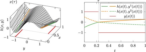
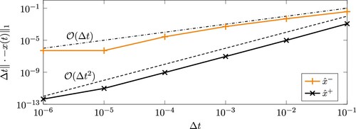
The results of the differential variable $x(t)$ are shown in Figure 3. The blue line represents the analytical solution, while the orange plus signs mark the numerical simulation without event detection and the black crosses mark the one with event detection (and location). It becomes visible that the differential variable is nonsmooth at the event. In Figure 4 the convergence behaviour of the numerical simulations with (black, cross) and without (orange, plus) explicit treatment of the event is plotted for decreasing time steps. It can be seen that the version with explicit treatment converges quadratically to the analytical solution, while the version without explicit treatment only converges linearly. Computing the event location and treating this explicitly in the simulation is only possible due to the tracking and detection of switches in the global optimum.

Figure 3. Analytical (line) and numerical (marks) results for differential variable $x(t)$ of Example 5.1. The differential equation is solved by trapezoidal rule with $\mathrm{\Delta }t=0.02$ without (superscript −) and with (superscript +) explicit treatment of events.

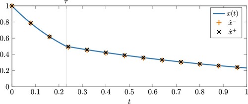
Figure 4. Convergence behaviour of the simulation from Example 5.1 without (superscript −) and with (superscript +) explicit treatment of events.

Example 5.2

The second DAEO considers a 1D Griewank inspired function [10] as embedded optimization problem. The DAEO is described by $\begin{array}{rl}x(0)& =1\\ x^{\prime }(t)& =y(x(t))\\ y(x(t))& \in {\arg \min }_y(y-x(t){)}^2+\sin (\mathrm{Cy}),\end{array}$with C = 5 and T = 2. The objective function has multiple optima that are emerging and vanishing over time. A surface plot of the function with the global optimizer $y(x(t))$ (red line) is given in Figure 5. It can be seen that there are four events on the time interval $t\in [0,2]$. 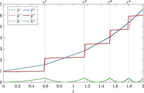The differentiable variable x (blue), the global optimizer y (red) and the global optimum $h(x,y)$ (green) are represented as lines in Figure 6. The numerical results of the version without (dashed) explicit treatment of the event differ slightly from the result with explicit treatment. This is a result of the error propagation due to the behaviour of the dynamic system.

Figure 5. Surface plot of the 1D Griewank inspired function from Example 5.2 with global optimizer (red line).

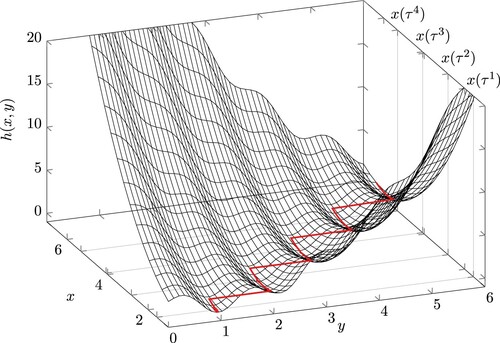
Figure 6. Differential variable x (blue), global optimizer y (red) and value of the global optimum (green) of Example 5.2 for the version with (solid) and without (dashed) explicit treatment of events.

6. Conclusions and further work

We introduced event detection and event location for a jumping global optimizer. The explicit treatment of events and its implementation into the numerical integrator yield a second-order convergent method for DAEOs in the presence of a jumping global optimizer. The second-order integrator enables the computation of discrete tangent and adjoint sensitivities of the dynamic system with respect to some parameters, which is crucial for solving optimal control problems of DAEOs. These sensitivities can now be obtained by AD methods.

Due to the high computational cost that comes along with the application of DGO in every time step, we aim for tracking relevant local optima in time instead. The global search is only required for getting a list of local optima and for recognizing that a new local optimum emerged during a time step. Vanishing optima should not be a problem with this approach.

Disclosure statement

No potential conflict of interest was reported by the author(s).

Additional information

Funding

This work was supported by the German Research Foundation (DFG) under grant number NA487/8-2.

Notes on contributors

Jens Deussen

Jens Deussen received his PhD degree in Applied Mathematics in 2022 from the RWTH Aachen University, Germany. The thesis title is 'Global Derivatives'. His research interests are algorithmic differentiation, adjoint methods in computational finance, deterministic global optimization and sparse matrices.

Jonathan Hüser

Jonathan Hüser received his PhD degree in 2022 from the RWTH Aachen University, Germany. The thesis title is 'Discrete Tangent and Adjoint Sensitivity Analysis for Discontinuous Solutions of Hyperbolic Conservation Laws'. His research interests are generalized differentiability in algorithmic differentiation for non-smooth optimization, uncertainty quantification and propagation and global optimization via convex relaxation.

Uwe Naumann

Uwe Naumann has been a professor in Computer Science at RWTH Aachen University, Aachen, Germany since 2004 and the Principal Scientist of the Numerical Algorithms Group (NAG) Ltd., Oxford, UK since 2022. He holds a PhD in Applied Mathematics from the Technical University, Dresden, Germany. His research and software development is largely inspired by algorithmic differentiation including applications in various areas of computational science, engineering and finance.

References

- L.E. Baker, A.C. Pierce, and K.D. Luks, Gibbs energy analysis of phase equilibria, SPE J. 22 (1982), pp. 731–742.
- D. Bongartz, J. Najman, S. Sass, and A. Mitsos, MAiNGO—McCormick-based algorithm for mixed-integer nonlinear global optimization, Technical report, Process Systems Engineering (AVT.SVT), RWTH Aachen University, 2018. Available at: http://www.avt.rwth-aachen.de/global/show_document.asp?id=aaaaaaaaabclahw.
- S.P. Boyd and L. Vandenberghe, Convex Optimization, Cambridge University Press, Cambridge, 2004.
- L.T. Biegler, Nonlinear Programming—Concepts, Algorithms, and Applications to Chemical Processes, SIAM, Philadelphia, PA, 2010.
- Y. Cao, S. Li, L. Petzold, and R. Serban, Adjoint sensitivity analysis for differential-algebraic equations: The adjoint DAE system and its numerical solution, SIAM J. Sci. Comput. 24 (2003), pp. 1076–1089.
- J. Deussen and U. Naumann, Efficient computation of sparse higher derivative tensors, in Computational Science—ICCS 2019—19th International Conference, Faro, Portugal, June 12–14, 2019, pp. 3–17.
- J. Deussen, J. Hüser, and U. Naumann, Toward global search for local optima, in Operations Research Proceedings 2019, J.S. Neufeld, U. Buscher, R. Lasch, D. Möst, and J. Schönberger, eds., Springer, Cham, 2020, pp. 97–104.
- J. Deussen, Global derivatives, Ph.D. diss., RWTH Aachen University, 2021.
- V. Gopal and L.T. Biegler, Smoothing methods for complementarity problems in process engineering, AlChE J. 45 (1999), pp. 1535–1547.
- A. Griewank, Generalized descent for global optimization, J. Optim. Theory Appl. 34 (1981), pp. 11–39.
- A. Griewank and A. Walther, Evaluating Derivatives: Principles and Techniques of Algorithmic Differentiation, SIAM, Philadelphia, PA, 2008.
- A. Griewank, On stable piecewise linearization and generalized algorithmic differentiation, Optim. Methods Softw. 28 (2013), pp. 1139–1178.
- A. Griewank, A. Walther, S. Fiege, and S. T. Bosse, On Lipschitz optimization based on gray-box piecewise linearization, Math. Program. 158 (2016), pp. 383–415.
- A. Griewank, R. Hasenfelder, M. Radons, L. Lehmann, and T. Streubel, Integrating Lipschitzian dynamical systems using piecewise algorithmic differentiation, Optim. Methods Softw. 33 (2018), pp. 1089–1107.
- E. Hansen and G.W. Walster, Global Optimization Using Interval Analysis, Marcel Dekker, New York, 2004.
- J.L. Hjersted and M.A. Henson, Optimization of fed-batch Saccharomyces cerevisiae fermentation using dynamic flux balance models, Biotechnol. Progr. 22 (2006), pp. 1239–1248.
- J. Hüser, Discrete tangent and adjoint sensitivity analysis for discontinuous solutions of hyperbolic conservation laws, Ph.D. diss., RWTH Aachen University, 2022.
- A. Khajavirad and N.V. Sahinidis, A hybrid LP/NLP paradigm for global optimization relaxations, Math. Program. Comput. 10 (2018), pp. 383–421.
- R. Mannshardt, One-step methods of any order for ordinary differential equations with discontinuous right-hand sides, Numer. Math. 31 (1978), pp. 131–152.
- G.P. McCormick, Computability of global solutions to factorable nonconvex programs: Part I—convex underestimating problems, Math. Program. 10 (1976), pp. 147–175.
- A. Mitsos, B. Chacuat, and P.I. Barton, McCormick-based relaxations of algorithms, SIAM J. Optim.20 (2009), pp. 573–601.
- R.E. Moore, Interval Analysis, Prentice Hall, Englewood Cliff, NJ, 1966.
- R.E. Moore, R.B. Kearfott, and M.J. Cloud, Introduction to Interval Analysis, SIAM, Philadelphia, PA, 2009.
- U. Naumann, The Art of Differentiating Computer Programs: An Introduction to Algorithmic Differentiation, SIAM, Philadelphia, PA, 2012.
- T. Park and P.I. Barton, State event location in differential-algebraic models, ACM Trans. Model. Comput. Simul. (TOMACS) 6 (1996), pp. 137–165.
- T. Ploch, E. von Lieres, W. Wiechert, A. Mitsos, and R. Hannemann-Tamás, Simulation of differential-algebraic equation systems with optimization criteria embedded in Modelica, Comput. Chem. Eng. 140 (2020), p. 106920.
- T. Ploch, J. Deussen, U. Naumann, A. Mitsos, and R. Hannemann-Tamás, Direct single shooting for dynamic optimization of differential-algebraic equation systems with optimization criteria embedded, Comput. Chem. Eng. 159 (2022), p. 107643.
- A.U. Raghunathan, M.S. Diaz, and L.T. Biegler, An MPEC formulation for dynamic optimization of distillation operations, Comput. Chem. Eng. 28 (2004), pp. 2037–2052.
- A.M. Sahlodin, H.A. Watson, and P.I. Barton, Nonsmooth model for dynamic simulation of phase changes, AIChE J. 62 (2016), pp. 3334–3351.