Adventures in Supersingularland

Abstract

Supersingular Isogeny Graphs were introduced as a source of hard problems in cryptography by Charles, Goren, and Lauter [6] for the construction of cryptographic hash functions and have been used for key exchange SIKE. The security of such systems depends on the difficulty of finding a path between two random vertices. In this article, we study several aspects of the structure of these graphs. First, we study the subgraph given by j-invariants in ${\mathbb{F}}_p$, using the related isogeny graph consisting of only ${\mathbb{F}}_p$-rational curves and isogenies. We prove theorems on how the connected components thereof attach, stack, and fold when mapped into the full graph. The ${\mathbb{F}}_p$-rational vertices are fixed by the Frobenius involution on the graph, and we call the induced graph the spine. Finding paths to the spine is relevant in cryptanalysis. Second, we present numerous computational experiments and heuristics relating to the position of the spine within the whole graph. These include studying the distance of random vertices to the spine, estimates of the diameter of the graph, how often paths are preserved under the Frobenius involution, and what proportion of vertices are conjugate. We compare some of the heuristics with known results on other Ramanujan graphs.

Keywords:

• elliptic curves
• diameters
• supersingular isogeny graphs

1 Introduction

Supersingular Isogeny Graphs have been the subject of recent study due to their significance in recently proposed post-quantum cryptographic protocols. In 2006, Charles, Goren, and Lauter proposed a hash function based on the hardness of finding paths (routing) in Supersingular Isogeny Graphs [6]. A few years later, De Feo, Jao, and Plût proposed a key exchange based on Supersingular Isogeny Graphs [12]. The security of most currently deployed cryptographic systems relies on either the hardness of factoring large integers of a certain form or the hardness of computing discrete logarithms in certain cyclic groups. Both problems can be efficiently solved using Shor’s algorithm [23] on a large-scale quantum computer once it exists. In 2015, NIST announced a contest to standardize cryptographic algorithms that are not known to be broken by quantum computers. Now in its third round, SIKE (https://sike.org/, based on Supersingular Isogeny Graphs) has been shortlisted as an alternate candidate.

To date, there are no known classical or quantum attacks that break the cryptographic protocols that use Supersingular Isogeny Graphs. But the graphs themselves have been relatively unstudied until recently. More study is needed before we can confidently recommend protocols which rely on the difficulty of the hard problem of finding paths in Supersingular Isogeny Graphs. There have been several approaches tried so far to attack cryptographic protocols based on Supersingular Isogeny Graphs. One of them uses the quaternion analogue of the graph and presents an efficient algorithm for navigating between maximal orders [18]. This approach leads to the results presented in [13] showing that the hardness of the path finding problem is essentially equivalent to the hardness of computing endomorphism rings of supersingular elliptic curves.

For distinct primes p and $\mathcal{l}$, let ${\mathcal{G}}_{\mathcal{l}}({\overline{\mathbb{F}}}_p)$ denote the graph whose vertices are isomorphism classes of supersingular elliptic curves over ${\overline{\mathbb{F}}}_p$ and whose edges correspond to isogenies of degree $\mathcal{l}$ defined over ${\overline{\mathbb{F}}}_p$. The vertices can be labeled with the j-invariant of the curve, which is an ${\overline{\mathbb{F}}}_p$-isomorphism invariant. For $p\equiv 1\text{mod}12$ the graph ${\mathcal{G}}_{\mathcal{l}}({\overline{\mathbb{F}}}_p)$ is known to be a $(\mathcal{l}+1)$-regular Ramanujan graph, and is one of two known families of Ramanujan graphs.

In this article, we study two related graphs to help understand the structure of ${\mathcal{G}}_{\mathcal{l}}({\overline{\mathbb{F}}}_p)$. First, the full subgraph of ${\mathcal{G}}_{\mathcal{l}}({\overline{\mathbb{F}}}_p)$ consisting of only vertices $j\in {\mathbb{F}}_p$: We denote this subgraph by $\mathcal{S}$ and call it the spine, which is new terminology. Second, we look at the graph ${\mathcal{G}}_{\mathcal{l}}({\mathbb{F}}_p)$ whose vertices are elliptic curves up to ${\mathbb{F}}_p$-isomorphism and edges are ${\mathbb{F}}_p$-isogenies of degree $\mathcal{l}$, already studied by Delfs and Galbraith [11].

We were motivated to continue the study of the graph ${\mathcal{G}}_{\mathcal{l}}({\mathbb{F}}_p)$ for several reasons. First, subexponential quantum algorithms are known for navigating between ${\mathbb{F}}_p$-vertices [3], so paths to these vertices are of particular interest. Second, the graph ${\mathcal{G}}_{\mathcal{l}}({\mathbb{F}}_p)$ maps into the full ${\mathcal{G}}_{\mathcal{l}}({\overline{\mathbb{F}}}_p)$ to become the spine in a surprising way, which we study in detail. Third, the Frobenius map acts on the full graph by sending each j-invariant in ${\mathbb{F}}_{p^2}$ to its ${\mathbb{F}}_p$ conjugate j^p, and the vertices in the spine are the fixed points of this involution. If we have a path from a random j-invariant to a j-invariant $j\prime$ in ${\mathbb{F}}_p$, then applying the involution to the vertices in the path we obtain a mirror path from $j\prime$ to j^p.

In Section 3 of this article, we compare ${\mathcal{G}}_{\mathcal{l}}({\mathbb{F}}_p)$ with the spine $\mathcal{S}$. The main results of Section 3 show how the components of ${\mathcal{G}}_{\mathcal{l}}({\mathbb{F}}_p)$ (which look like volcanoes) fit together to form the spine when passing to the full graph ${\mathcal{G}}_{\mathcal{l}}({\overline{\mathbb{F}}}_p)$. We define the notions of stacking, folding, and attaching to describe how ${\mathcal{G}}_{\mathcal{l}}({\mathbb{F}}_p)$ becomes the spine, when isogenies defined over ${\overline{\mathbb{F}}}_p$ are added and j-invariants which are twists are identified. We achieve this by comparing the possible neighbors of the vertices in ${\mathcal{G}}_{\mathcal{l}}({\mathbb{F}}_p)$ that have the same j-invariant. We prove that the only vertices that do not have the same neighbors are those with $\mathbf{j}=1728$ (Lemma 3.17 and Proposition 3.22).

For $\mathcal{l}>2$, for odd class numbers, we show that the number of edges in $\mathcal{S}$ that do not come from isogenies defined over ${\mathbb{F}}_p$ is bounded by $4{\mathcal{l}}^2$ and for any p, this bound can be sharpened for any $\mathcal{l}$, based on congruence conditions on p. Further, we show that the components containing $\mathbf{j}=1728$ are “symmetric” and the opposite vertices of $\mathbf{j}=1728$ form a pair of $\mathcal{l}$-isogenous quadratic twists, whereas all other components admit a “twist twin”: a component that is isomorphic to it as labeled graphs if we label the vertices by the j-invariants of the curves (Theorem 3.18).

For $\mathcal{l}=2$, we provide a similar analysis. Again, the component containing 1728 is “symmetric” and all other components admit a “twist twin,” except for the case of one edge $[8000,8000]$. Moreover, in this case, at most 2 new edges are added that do not correspond to loops and we identify at which vertices these can occur.

We conclude that for any fixed $\mathcal{l}$ and p, the resulting shape of the spine depends on the congruence class of p, the structure of the class group $\text{cl}({\mathcal{O}}_K)$, where $K=\mathbb{Q}\left(\sqrt{-p}\right)$, and the behavior of the prime above $\mathcal{l}$ in the class group of K, and we show how to determine it explicitly. In Section 3.5, we generate experimental data to study how the components of the spine are distributed throughout the graph and we estimate how many components there are in the spine.

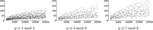
In Section 4.1, we study the distance between Galois conjugate pairs of vertices, that is, pairs of $\mathit{j}$-invariants of the form $\mathit{j}$, ${\mathit{j}}^p$. Our data suggest these vertices are closer to each other than a random pair of vertices in ${\mathcal{G}}_2({\overline{\mathbb{F}}}_p)$. In Section 4.2 we test how often the shortest path between two conjugate vertices goes through the spine $\mathcal{S}$, or equivalently, contains a j-invariant in ${\mathbb{F}}_p$. We find conjugate vertices are more likely than a random pair of vertices to be connected by a shortest path through the spine. Finally, we examine the distance between arbitrary vertices and the spine $\mathcal{S}$ in Section 4.3. Section 5 provides heuristics on how often conjugate $\mathit{j}$-invariants are $\mathcal{l}$-isogenous for $\mathcal{l}=2,3$, a question motivated by the study of mirror paths provided in Section 4.

Another family of Ramanujan graphs are certain Cayley graphs constructed by Lubotzky, Philips, and Sarnak (LPS graphs [20]). The relationship between LPS graphs and Supersingular Isogeny Graphs is studied in [5]. Sardari [22] provides an analysis of the diameters of LPS graphs, and in Section 6 of this article, we provide heuristics and a discussion of the diameters of supersingular 2-isogeny graphs.

Our experiments and data suggest a noticeable difference in the Supersingular Isogeny Graphs ${\mathcal{G}}_{\mathcal{l}}({\overline{\mathbb{F}}}_p)$ depending on the congruence class of the prime $p\text{mod}12$. It has been known since the introduction of Supersingular Isogeny Graphs into cryptography [6] that the congruence class of the prime p has an important role to play in the properties of the graph. In particular, it was shown there how the existence of short cycles in the graph depends explicitly on the congruence conditions on p. In this article, we extend this observation and find significant differences in the graphs depending on the congruence class of p. In summary, the data seem to suggest the following:

• $p\equiv 1\text{mod}12$:

  • smaller 2-isogeny graph diameters (Section 6.1),

  • larger number of spinal components (Section 3.6), and

  • larger proportion of 2-isogenous conjugate pairs (Section 5.2.1),

• $p\equiv 11\text{mod}12$:

  • larger 2-isogeny graph diameters,

  • smaller number of spinal components, and

  • smaller proportion of 2-isogenous conjugate pairs.

To accompany the experimental results of this article, we have made the Sage code for all the computations available, along with a short discussion of the different algorithms included. The code is posted at https://github.com/krstnmnlsn/Adventures-in-Supersingularland-Data.

1.1 Related work

Adj, Ahmadi, and Menezes [1] were the first to study the fine structure of the graph ${\mathcal{G}}_{\mathcal{l}}({\overline{\mathbb{F}}}_p)$. In particular, they studied ${\mathcal{G}}_{\mathcal{l}}({\mathbb{F}}_{p^2},t)$, which is the graph whose vertices are elliptic curves with fixed trace of Frobenius t and whose edges are ${\mathbb{F}}_{p^2}$-isogenies. They showed that the graph ${\mathcal{G}}_{\mathcal{l}}({\mathbb{F}}_{p^2},-2p)$ is isomorphic as a graph to ${\mathcal{G}}_{\mathcal{l}}({\overline{\mathbb{F}}}_p)$. Our approach in the current article also studies a subclass of curves and the paths passing through these curves. After our preprint appeared [2], a related approach was introduced by Boneh and Love [4] to study a subgraph which contains supersingular curves with small non-integer endomorphisms. Such small endomorphisms can be used to efficiently compute isogenies between the special curves.

Shortly after our work was first posted [2], Castryck, Panny, and Vercauteren posted a article on rational isogenies [10]. Their work gives an algorithm for computing an ideal to connect two supersingular elliptic curves over ${\mathbb{F}}_p$ which have the same ${\mathbb{F}}_p$-endomorphism ring. Their focus on ${\mathbb{F}}_p$-curves is parallel to our results regarding the structure of the ${\mathbb{F}}_p$ isogeny graph ${\mathcal{G}}_{\mathcal{l}}({\mathbb{F}}_p)$ and the spine $\mathcal{S}$.

More recently, Eisentraeger et al. [14] gave a cycle finding algorithm to compute endomorphism rings of supersingular elliptic curves. A key part of their algorithm involves finding j-invariants that are $\mathcal{l}$-isogenous to their conjugates. Since this is done by performing random walks, they determine a lower bound for the size of the set of such j-invariants. This gives a partial answer to our Question 3 in Section 5.

2 Definitions

Let k be a finite field of characteristic $p>3$ and let E be an elliptic curve over k. We may assume that is given by an equation $y^2=x^3+ax+b$ for some $a,b\in k$ (and such that $x^3+ax+b$ does not have a multiple root). A point on E is simply given by its coordinates (x_P, y_P) for $x_P,y_P\in \overline{k}$. Elliptic curves have a group law given by algebraic formulas that can be efficiently computed. Moreover, the number of points in these groups can be counted fast, which makes them both particularly rich objects to work with and very handy objects for cryptographic constructions.

We focus on supersingular elliptic curves: Curves E/k with endomorphism ring ${\text{End}}_{{\overline{\mathbb{F}}}_p}(E)$ a maximal order in a quaternion algebra. Equivalent definitions can be found in [24, Theorem V.3.1]. Endomorphism rings of elliptic curves with j-invariant in ${\mathbb{F}}_p$ are characterized in [11, Prop. 2.4]: for p > 3, a supersingular elliptic curve $E/{\overline{\mathbb{F}}}_p$ can be defined over ${\mathbb{F}}_p$ if and only if $\mathbb{Z}[\sqrt{-p}]\subset \text{End}(E)$.

Supersingular elliptic curves can all be identified with a j-invariant in ${\mathbb{F}}_{p^2}$. We will use the notation E_j to fix an elliptic curve with j-invariant j. The j-invariants classify the ${\overline{\mathbb{F}}}_p$-isomorphism classes of supersingular elliptic curves. When we instead consider supersingular elliptic curves with $j(E)\in {\mathbb{F}}_p$ up to ${\mathbb{F}}_p$-isomorphism, two ${\mathbb{F}}_p$-isomorphism classes share the same j-invariant [11, Prop. 2.3]. One can distinguish between the two classes by the Weierstrass models of the elliptic curves.

2.1 Isogeny graphs

To introduce the graphs, we borrow the following notions from Sutherland [25, Section 2.2]. We denote by ${\Phi }_{\mathcal{l}}(X,Y)$ the $\mathcal{l}$-modular polynomial. We let E_j denote an elliptic curve of j-invariant j, up to ${\overline{\mathbb{F}}}_p$ isomorphism. This is a polynomial of degree $\mathcal{l}+1$ in both X and Y, symmetric in X and Y, and such that there exists a cyclic $\mathcal{l}$-isogeny $\varphi :E_{j_1}\to E_{j_2}$ if and only if ${\Phi }_{\mathcal{l}}(j_1,j_2)=0$.

In principle, the modular polynomials can be computed and they are accessible via tables for small values of $\mathcal{l}$. However, their coefficients are rather large, as we see already for ${\Phi }_2(X,Y)$:(1) $$\begin{array}{cc}{\Phi }_2(X,Y)=\hfill & -X^2{Y}^2+X^3+1488X^{2}Y+1488X{Y}^2+Y^3-162000X^2\hfill \\ \hfill & +40773375XY-162000Y^2+8748000000X+8748000000Y\hfill \\ \hfill & -157464000000000\hfill \end{array}$$(1)

A separable isogeny is determined by its kernel [24]. In addition, we will need the notion of equivalence of isogenies:

Definition 2.1

(Equivalent isogenies). Let k be a field. We say two separable isogenies $\phi ,\phi \prime$ between k-isomorphism classes of elliptic curves are equivalent if $\phi \prime =\psi °\phi$, for some automorphism ψ of the codomain.

Notice that equivalent isogenies share the same kernel, and inequivalent isogenies from E correspond to distinct roots of ${\Phi }_{\mathcal{l}}(j(E),Y)=0$.

Definition 2.2

(Supersingular $\mathcal{l}$-isogeny graph over ${\overline{\mathbb{F}}}_p$: ${\mathcal{G}}_{\mathcal{l}}({\overline{\mathbb{F}}}_p)$). The graph ${\mathcal{G}}_{\mathcal{l}}({\overline{\mathbb{F}}}_p)$ has vertex set ${\overline{\mathbb{F}}}_p$-isomorphism classes of supersingular elliptic curves over ${\overline{\mathbb{F}}}_p$, labeled by their j-invariants in ${\mathbb{F}}_{p^2}$. There is a directed edge from vertex j to $j\prime$ for every root $j\prime$ of the modular polynomial ${\Phi }_{\mathcal{l}}(j,Y)$, considered with multiplicity.

We label the vertices of ${\mathcal{G}}_{\mathcal{l}}({\overline{\mathbb{F}}}_p)$ with j-invariants but sometimes it is more convenient to talk about elliptic curves. By definition, every edge $[j,j\prime ]$ corresponds to an $\mathcal{l}$-isogeny $E_j\to E_{j\prime }$ for any choice of E_j and $E_{j\prime }$.

Remark 2.3.

Every vertex in this graph has outgoing degree $\mathcal{l}+1$, however, vertices with j-invariant $\mathbf{j}=0$ or 1728 have fewer incoming edges (due to automorphisms). Identifying isogenies with their dual isogenies makes this graph undirected and $(\mathcal{l}+1)$-regular except at those vertices or their neighbors. The graphs displayed in this article are pictured as undirected, so we expect irregularities in these figures at j = 0, 1728.

The isogeny graphs ${\mathcal{G}}_{\mathcal{l}}({\overline{\mathbb{F}}}_p)$ are Ramanujan graphs for $p\equiv 1\mathrm{mod}12$ (see [7]). Kohel [19, Ch. 7] proved that every pair of supersingular elliptic curves are connected by a chain of $\mathcal{l}$-isogenies, which implies that the graph is connected. If p > 3, the number of vertices of ${\mathcal{G}}_{\mathcal{l}}({\overline{\mathbb{F}}}_p)$ is $\approx \frac{p}{12}$, depending on the congruence class of $p\text{mod}12$ [24, Section V.4].

If j is a supersingular j-invariant, then so is its ${\mathbb{F}}_{p^2}$-conjugate j^p. Moreover, because modular polynomials have integer coefficients, if j and $j\prime$ satisfy ${\Phi }_{\mathcal{l}}(j,j\prime )=0$ then also (in ${\overline{\mathbb{F}}}_p$)$${\Phi }_{\mathcal{l}}(j^p,{(j\prime )}^p)={({\Phi }_{\mathcal{l}}(j,j\prime ))}^p=0.$$

This means that for any edge $[j,j\prime ]\in {\mathcal{G}}_{\mathcal{l}}({\overline{\mathbb{F}}}_p)$, there is a mirror edge $[j^p,{(j\prime )}^p]$.

This leads to the idea of a mirror involution on ${\mathcal{G}}_{\mathcal{l}}({\overline{\mathbb{F}}}_p)$:

Definition 2.4.

The mirror involution on ${\mathcal{G}}_{\mathcal{l}}({\overline{\mathbb{F}}}_p)$ is the map defined by sending the vertex represented by $j\in {\mathbb{F}}_{p^2}$ to the vertex represented by j^p.

A vertex $j\in {\mathcal{G}}_{\mathcal{l}}({\overline{\mathbb{F}}}_p)$ is fixed under the mirror involution if and only if $j\in {\mathbb{F}}_p$. We are interested in the subgraph of ${\mathcal{G}}_{\mathcal{l}}({\overline{\mathbb{F}}}_p)$ induced by these vertices:

Definition 2.5

(Spine). The spine is the induced subgraph $\mathcal{S}$ of ${\mathcal{G}}_{\mathcal{l}}({\overline{\mathbb{F}}}_p)$ consisting of all vertices whose j-invariants lie in ${\mathbb{F}}_p$ and all edges between them in ${\mathcal{G}}_{\mathcal{l}}({\overline{\mathbb{F}}}_p)$.

Note that many of the edges do correspond to isogenies defined over ${\mathbb{F}}_p$ but there can be edges coming from isogenies only defined over ${\overline{\mathbb{F}}}_p$. In Section 3, we determine all possible such edges.

The number of vertices in the spine $\mathcal{S}$ depends on the class number of the imaginary quadratic field $\mathbb{Q}\left(\sqrt{-p}\right)$ and is of size $\tilde{O}\left(\sqrt{p}\right)$. The size, shape and number of connected components of the spine $\mathcal{S}$ will be studied in Section 3.

To study the spine, we introduce some notation that will help keep track of whether the j-invariants we are studying are defined over ${\mathbb{F}}_p$ or not: Whenever we want to stress that a j-invariant of an elliptic curve lies in ${\mathbb{F}}_p$, we use bold letters (such as j). If we want to stress that a particular j-invariant lies in ${\mathbb{F}}_{p^2}\setminus {\mathbb{F}}_p$, we will use the more curly bold $\mathit{j}$.

We were motivated to study the spine because the ${\mathbb{F}}_p$ vertices may play a role in attacks on Supersingular Isogeny Graph-based cryptosystems. In [11], Delfs and Galbraith construct an isogeny between two supersingular elliptic curves by first finding an isogeny from each curve to a curves whose j-invariant lies in ${\mathbb{F}}_p$, and then constructing an isogeny between the curves in ${\mathbb{F}}_p$. They argue that while taking random walks in ${\mathcal{G}}_{\mathcal{l}}({\overline{\mathbb{F}}}_p)$, one can find elements in $\mathcal{S}$ with probability given (roughly) by the size of the subgraph divided by the size of the full isogeny graph. However, we will see in Section 3 that there is still a lot of structure in $\mathcal{S}$ that cannot be discounted.

In Sections 4 and 5, we then investigate other questions relating to whether the spine $\mathcal{S}$ is close to a random subgraph or whether the bountiful structure of the spine $\mathcal{S}$ is visible inside the Supersingular Isogeny Graph ${\mathcal{G}}_{\mathcal{l}}({\overline{\mathbb{F}}}_p)$.

To explain the terminology ‘spine’: Starting from $\mathcal{S}$, we can construct ${\mathcal{G}}_{\mathcal{l}}({\overline{\mathbb{F}}}_p)$ by adding j-invariants in conjugate pairs: starting with j in $\mathcal{S}$, if there is an isogeny from $E_{\mathbf{j}}$ to $E_{\mathit{j}}$, there is a conjugate isogeny from $E_{\mathbf{j}}$ to the conjugate $E_{{\mathit{j}}^{(p)}}$. Hence we imagine the ‘spine’ as being the backbone of the Supersingular Isogeny Graph ${\mathcal{G}}_{\mathcal{l}}({\overline{\mathbb{F}}}_p)$.

Definition 2.6.

We say that a path P with vertices $\{j_0,j_1,j_2,\dots ,j_{n-1},j_n\}$ (considered as an undirected path) is a mirror path if it is invariant under the mirror involution.

There exists at least one mirror path between any two conjugate j-invariants: it suffices to find a path from one j-invariant, say ${\mathit{j}}_0$, to an ${\mathbb{F}}_p$ j-invariant and then conjugate this path.

In general, mirror paths have either the form$${\mathit{j}}_0\to {\mathit{j}}_1\to \cdots \to {\mathit{j}}_n\to \mathbf{j}\to {\mathit{j}}_n^p\to \cdots \to {\mathit{j}}_1^p\to {\mathit{j}}_0^p,$$passing through an ${\mathbb{F}}_p$-vertex, or$${\mathit{j}}_0\to {\mathit{j}}_1\to \cdots \to {\mathit{j}}_n\to {\mathit{j}}_n^p\to \cdots \to {\mathit{j}}_1^p\to {\mathit{j}}_0^p,$$ passing through a pair of conjugate j-invariants.

2.2 Special j-invariants

In this section, we discuss j-invariants with special properties which require attention in the discussions to follow, focusing on j-invariants with extra automorphisms and then on j-invariants that are contained in very short cycles in ${\mathcal{G}}_{\mathcal{l}}({\mathbb{F}}_p)$: self-loops and cycles of length 2 (double edges).

2.2 Automorphisms

First, $\mathbf{j}=1728$ and $\mathbf{j}=0$ correspond to curves with extra automorphisms, which make the graph ${\mathcal{G}}_{\mathcal{l}}({\overline{\mathbb{F}}}_p)$ undirected (see Remark 2.3). The j-invariant $\mathbf{j}=1728$ is supersingular if and only if $p\equiv 3\text{mod}4$ and $\mathbf{j}=0$ is supersingular if and only if $p\equiv 2\text{mod}3$ (see [24, Chapter V]).

2.2 Loops

Loops in the graph ${\mathcal{G}}_{\mathcal{l}}({\overline{\mathbb{F}}}_p)$ are easily read off from the factorization of ${\Phi }_{\mathcal{l}}(X,X)$: a vertex represented by a j-invariant j admits a loop if and only if ${\Phi }_{\mathcal{l}}(j,j)=0$. For $\mathcal{l}=2$, factoring over $\mathbb{Z}$ the polynomial ${\Phi }_2(X,X)$ from (1) we get:(2) $${\Phi }_2(X,X)=-{(X+3375)}^2(X-1728)(X-8000).$$(2)

Therefore, loops in ${\mathcal{G}}_2({\overline{\mathbb{F}}}_p)$ are only possible at the vertices $\mathbf{j}=-3375$ (two loops), $\mathbf{j}=1728$ (one loop, explained in Example 3.8) and $\mathbf{j}=8000$ (one loop). These j-invariants need not be supersingular for a particular prime p, so they do not always appear in ${\mathcal{G}}_2({\overline{\mathbb{F}}}_p)$.

2.2 Double edges

The following lemma describes double edges in the $\mathcal{l}$-isogeny graph. This lemma applies mutatis mutandis for ordinary curves, replacing ${\mathcal{G}}_{\mathcal{l}}({\overline{\mathbb{F}}}_p)$ by the $\mathcal{l}$-isogeny graph of ordinary elliptic curves.

Lemma 2.7

(Double edge lemma). If two j-invariants j₁, j₂ in the $\mathcal{l}$-isogeny graph ${\mathcal{G}}_{\mathcal{l}}({\overline{\mathbb{F}}}_p)$ have a double-edge between them, then j₁ and j₂ are both roots of the polynomial (3) $${\text{Res}}_{\mathcal{l}}(X):=\mathrm{Res}\left({\Phi }_{\mathcal{l}}(X,Y),\frac{d}{dY}{\Phi }_{\mathcal{l}}(X,Y);Y\right).$$(3)

The degree of ${\text{Res}}_{\mathcal{l}}(X)$ is bounded by $2\mathcal{l}·(2\mathcal{l}-1)$.

Proof.

Suppose that j₁ and j₂ are two vertices in the $\mathcal{l}$-isogeny graph connected with a double edge. Considered as a polynomial in Y, the polynomial ${\Phi }_{\mathcal{l}}(j_1,Y)={(Y-j_2)}^2·g(j_1,Y)$ for some $g(j_1,Y)\in {\overline{\mathbb{F}}}_p[Y]$. The derivative $\frac{d}{dY}{\Phi }_{\mathcal{l}}(j_1,Y)$ with respect to Y then also vanishes at $Y=j_2$. The polynomials ${\Phi }_{\mathcal{l}}(X,Y)$ and $\frac{d}{dY}{\Phi }_{\mathcal{l}}(X,Y)$ share the root X = j₁, and so by definition j₁ is a root of the resultant ${\mathrm{Res}}_{\mathcal{l}}(X)$. This argument is also true for j₂, so j₂ is also a root of ${\mathrm{Res}}_{\mathcal{l}}(X)$.

The total degree of ${\Phi }_{\mathcal{l}}(X,Y)$ is $2\mathcal{l}$ and the total degree of $\frac{d}{dY}{\Phi }_{\mathcal{l}}(X,Y)$ is $2\mathcal{l}-1$. Since the resultant of two polynomials P(X, Y) and Q(X, Y) of total degrees d and e generically has degree $d·e$, we obtain the bound $\#\{j:\mathrm{}\text{there}\mathrm{}\text{is}\text{a}\text{double}\mathrm{}\text{edge}\mathrm{}\text{from}\mathrm{}j\}\le 2\mathcal{l}·(2\mathcal{l}-1).$ □

Example 2.8

(Double edges for $\mathcal{l}=2$). For $\mathcal{l}=2$, we can factor the resultant over $\mathbb{Z}$ as follows:(4) $${\text{Res}}_2(X)=-2^2·X^2·(X-1728)·{(X+3375)}^2·{(X^2+191025X-121287375)}^2$$(4)

Therefore, any double edge in ${\mathcal{G}}_2({\overline{\mathbb{F}}}_p)$ can only appear between j-invariants from this list: $0,1728,-3375$ or a root of $X^2+191025X-121287375$.

By factoring ${\Phi }_2(j,X)$ for these values, we can for instance see that $\mathbf{j}=0$ is the only j-invariant that admits a triple edge in ${\mathcal{G}}_2({\overline{\mathbb{F}}}_p)$.

Remark 2.9

(Short cycles and tightness of the bound). Note that the bound on the degree in Lemma 2.7 is not tight. For example for $\mathcal{l}=2$, the bound is 12 whereas the polynomial has degree 9. A sharper estimate could be obtained as a sum of class numbers using an approach from [6] as follows. A double edge in ${\mathcal{G}}_{\mathcal{l}}({\overline{\mathbb{F}}}_p)$ gives a cycle of length 2 in the same graph. Short cycles were already studied in [6], where it was shown that for a fixed $\mathcal{l}$, the existence of short cycles depends on congruence conditions on p. A short cycle of length n corresponds to an element of norm ${\mathcal{l}}^n$ in the endomorphism rings of the curves whose j-invariants form this cycle. For instance, a double edge in ${\mathcal{G}}_2({\overline{\mathbb{F}}}_p)$ gives a non-trivial quadratic element of norm 4 in ${\text{End}}_{{\overline{\mathbb{F}}}_p}(E_j)$. Elliptic curves defined over a number field with CM by an imaginary quadratic field K reduce to supersingular elliptic curves modulo p if p is inert in K. The only imaginary quadratic fields that contain an element of norm 4 are $\mathbb{Q}\left(\sqrt{-3}\right),\mathbb{Q}\left(\sqrt{-1}\right),\mathbb{Q}\left(\sqrt{-7}\right)$ and $\mathbb{Q}\left(\sqrt{-15}\right)$ and the factors of ${\text{Res}}_2(X)$ are the Hilbert class polynomials for these fields. So it is not surprising that the resultants ${\text{Res}}_{\mathcal{l}}$ factor as a product of Hilbert class polynomials for imaginary quadratic fields, and thus the degree of ${\text{Res}}_2(X)$ can be bounded by the sum of the class numbers of these imaginary quadratic fields. For any given $\mathcal{l}$, there are at most $2\mathcal{l}$ such imaginary quadratic fields possible, all with discriminant bounded by $4{\mathcal{l}}^2$. So to get a sharper bound on the degree, we only need to sum the class numbers of these quadratic fields.

3 Structure of the ${\mathbb{F}}_p$-subgraph: the spine $\mathcal{S}$

In this section, we investigate the shape of the spine $\mathcal{S}$, which was introduced in Definition 2.5 as the subgraph of ${\mathcal{G}}_{\mathcal{l}}({\overline{\mathbb{F}}}_p)$ consisting of the vertices defined over ${\mathbb{F}}_p$. The motivation for studying the structure of this subgraph is the existence of attacks on SIDH that work by finding ${\mathbb{F}}_p$ j-invariants. This idea was presented in [11], and a quantum attack based on it was given by Biasse, Jao and Sankar [3]. See also [15] for an overview of the security considerations for SIDH.

In Section 3.1, we start with the graph ${\mathcal{G}}_{\mathcal{l}}({\mathbb{F}}_p)$, the structure of which is understood well. We base our investigations on the study of ${\mathcal{G}}_{\mathcal{l}}({\mathbb{F}}_p)$ done by Delfs and Galbraith in [11].

Moreover, a version of the ${\mathbb{F}}_p$-graph (allowing edges corresponding to $\mathcal{l}$-isogenies for multiple primes) has also been proposed for post-quantum cryptography in [8]. We recall the results of [11] in some detail and give a few explicit examples of their results about endomorphisms of certain elliptic curves.

In Section 3.2, we discuss how the spine $\mathcal{S}$ can be obtained from ${\mathcal{G}}_{\mathcal{l}}({\mathbb{F}}_p)$ in two steps: first vertices corresponding to the same j-invariant are identified and then a few new edges are added. The possible ways the connected components can identify are given by Definition 1 and we call them stacking, folding, attaching along a j-invariant and attaching by a new edge.

In Section 3.3 we study stacking, folding and attaching for $\mathcal{l}>2$ and give an example of the theory we develop for $\mathcal{l}=3$ in Section 3.3.1. In this section we also give a complete description of stacking, folding and attaching in Theorem 3.21. We return to the case $\mathcal{l}=2$ in Section 3.4, giving a similar complete description in Theorem 3.29 and some data on how often attachment of distinct components happens. Section 3.5 contains some experimental data on the distances between the connected components of $\mathcal{S}\subset {\mathcal{G}}_2({\mathbb{F}}_p)$.

In this section, we assume that all elliptic curves are supersingular.

3.1 Structure of the ${\mathbb{F}}_p$-Graph ${\mathcal{G}}_{\mathcal{l}}({\mathbb{F}}_p)$

To study the spine $\mathcal{S}$, we will use the following isogeny graph ${\mathcal{G}}_{\mathcal{l}}({\mathbb{F}}_p)$ defined over ${\mathbb{F}}_p$, first studied by Delfs and Galbraith [11].

Definition 3.1

(Supersingular $\mathcal{l}$-isogeny graph over ${\mathbb{F}}_p$). The graph ${\mathcal{G}}_{\mathcal{l}}({\mathbb{F}}_p)$ has vertex set the ${\mathbb{F}}_p$-isomorphism classes of supersingular elliptic curves defined over ${\mathbb{F}}_p$. The edges correspond to ${\mathbb{F}}_p$-equivalence classes (in the sense of Definition 2.1) of $\mathcal{l}$-isogenies defined over ${\mathbb{F}}_p$.

For p > 3, each supersingular j-invariant corresponds to exactly two ${\mathbb{F}}_p$-isomorphism classes of curves. These curves can be distinguished by other invariants (such as the c₄ and c₆ values from [24, III.1]). We will use notation such as v_a and w_a to denote the vertices corresponding to the two twists with j-invariant a. For visualization, we will label the vertices of the graph ${\mathcal{G}}_{\mathcal{l}}({\mathbb{F}}_p)$ only by j-invariants.

Remark 3.2.

We highlight the differences between $\mathcal{S}$ and ${\mathcal{G}}_{\mathcal{l}}({\mathbb{F}}_p)$:

• $\mathcal{S}$ has half as many vertices as ${\mathcal{G}}_{\mathcal{l}}({\mathbb{F}}_p)$, since the vertices in the spine $\mathcal{S}$ are considered up to ${\overline{\mathbb{F}}}_p$-isomorphism and up to ${\mathbb{F}}_p$-isomorphism in the graph ${\mathcal{G}}_{\mathcal{l}}({\mathbb{F}}_p)$.

• $\mathcal{S}$ can have edges between j-invariants previously not connected in ${\mathcal{G}}_{\mathcal{l}}({\mathbb{F}}_p)$. However, we will show in Lemma 3.14 that this is a fairly rare occurrence.

We will use the equivalent definition of supersingularity for elliptic curves over ${\mathbb{F}}_p$ pointed out by [11]: an elliptic curve $E/{\mathbb{F}}_p$ is supersingular if and only if $\mathbb{Z}[\sqrt{-p}]\subset {\text{End}}_{{\mathbb{F}}_p}(E)$. If $p\equiv 3\text{mod}4$, the order $\mathbb{Z}[\sqrt{-p}]$ is strictly contained in the maximal order $\mathbb{Z}\left[\frac{1+\sqrt{-p}}{2}\right]$. It is convenient to distinguish these two cases:

Definition 3.3

(Surface and Floor). Let E be a supersingular elliptic curve over ${\mathbb{F}}_p$. We say E is on the surface (resp. E is on the floor) if $\mathrm{End}{\mathbb{F}}_p(E)={\mathcal{O}}_K$ (resp. $\mathrm{End}{\mathbb{F}}_p(E)=\mathbb{Z}[\sqrt{-p}]$).

Note that for $p\equiv 1\text{mod}4$, surface and floor coincide.

Definition 3.4

(Horizontal and Vertical Isogenies.). Let $\phi$ be an $\mathcal{l}$-isogeny between supersingular elliptic curves E and $E\prime$ over ${\mathbb{F}}_p$. If ${\mathrm{End}}_{{\mathbb{F}}_p}(E)\cong {\text{End}}_{{\mathbb{F}}_p}(E\prime )$ then $\phi$ is called horizontal. Otherwise, $\phi$ is called vertical.

The following is Theorem 2.7 of [11].

Theorem 3.5

(Structure of ${\mathcal{G}}_{\mathcal{l}}({\mathbb{F}}_p)$). Let p > 3 and $\mathcal{l}$ be primes.

1. For $\mathcal{l}>2$, there are no vertical isogenies. If $\left(\frac{-p}{\mathcal{l}}\right)=1$, then there are two horizontal $\mathcal{l}$-isogenies from each vertex and beyond this no other $\mathcal{l}$-isogenies. Hence every connected component of ${\mathcal{G}}_{\mathcal{l}}({\mathbb{F}}_p)$ is a cycle.

2. Case $p\equiv 1\text{mod}4$. There is one level in ${\mathcal{G}}_{\mathcal{l}}({\mathbb{F}}_p)$: all elliptic curves E have ${\text{End}}_{{\mathbb{F}}_p}(E)=\mathbb{Z}[\sqrt{-p}]$. For $\mathcal{l}=2$: from each vertex there is one outgoing 2-isogeny.

   There are $h(-4p)$ vertices on the surface (which coincides with the floor).

3. Case $p\equiv 3\text{mod}4$. There are two levels in ${\mathcal{G}}_{\mathcal{l}}({\mathbb{F}}_p)$: surface and floor. For $\mathcal{l}=2$:

   1. If $p\equiv 7\text{mod}8$, there is exactly one vertical isogeny from any vertex on the surface to a vertex on the floor, every vertex on the surface admits two horizontal isogenies and there are no horizontal isogenies between the curves on the floor.

      There are $h(-p)$ vertices on the floor and $h(-p)$ vertices on the surface.

   2. If $p\equiv 3\text{mod}8$, from every vertex on the surface, there are exactly three vertical isogenies to the floor, and there are no horizontal isogenies between any vertices.

      There are $3·h(-p)$ vertices on the floor and $h(-p)$ vertices on the surface.

This implies that every connected component of ${\mathcal{G}}_2({\mathbb{F}}_p)$ is an isogeny volcano, first studied by Kohel [19]. For a reference on the name and basic properties we refer to [25].

Let $K=\mathbb{Q}\left(\sqrt{-p}\right)$ and $\mathfrak{p}$ be a prime above $\mathcal{l}=2$ in ${\mathcal{O}}_K$, and $h=\#\text{cl}({\mathcal{O}}_K)$ the class number of K. Let n be the order of $\mathfrak{p}$ in $\text{cl}({\mathcal{O}}_K)$. The surface of any volcano in ${\mathcal{G}}_2({\mathbb{F}}_p)$ is a cycle of precisely n vertices. There are h/n connected components (volcanoes) in ${\mathcal{G}}_2({\mathbb{F}}_p)$, the index of $〈\mathfrak{p}〉$ in $\text{cl}({\mathcal{O}}_K)$.

The following lemma is due to [11].

Lemma 3.6.

Let p > 5. Let E be a supersingular elliptic curve defined over ${\mathbb{F}}_p$. Then $${\text{End}}_{{\mathbb{F}}_p}(E)=\mathbb{Z}\left[\frac{1+\sqrt{-p}}{2}\right]\mathit{\hspace{1em}if\; and\; only\; if\hspace{1em}E}\left[2\right]\subset \mathrm{E}({\mathbb{F}}_{\mathrm{p}}).$$

Note that for $p\equiv 1\text{mod}4$, the ring $\mathbb{Z}\left[\frac{1+\sqrt{-p}}{2}\right]$ is not an order of ${\mathcal{O}}_K$, so no supersingular elliptic curves in ${\mathbb{F}}_p$ have their full 2-torsion defined over ${\mathbb{F}}_p$.

We recall the following definition from [24]: a twist of an elliptic curve E over a field K is a curve $E\prime$ which is isomorphic to E over $\overline{K}$. Two twists are considered equivalent if they are isomorphic over K. The group of twists of a given elliptic curve is given by the standard formula in [24, Proposition X.5.4]. For the field ${\mathbb{F}}_p$, every supersingular j-invariant will have precisely two isomorphism classes of twists: Curves with j-invariant not equal to 1728 have two isomorphism classes of quadratic twists, and j = 1728 has two isomorphism classes of quartic twists.

The following corollary of Lemma 3.6 will be essential in our discussion in Section 3.4.

Corollary 3.7

(Endomorphism rings of quadratic twists). Let p > 3 be a prime, let E be an elliptic curve defined over ${\mathbb{F}}_p$ and let E^t denote its quadratic twist. Then $${\text{End}}_{{\mathbb{F}}_p}(E)\cong {\text{End}}_{{\mathbb{F}}_p}(E^t).$$

Proof.

Suppose $E:y^2=x^3+ax+b$. Then the quadratic twist is $E^t:y^2=x^3+d^{2}ax+d^{3}b$, where d is a quadratic non-residue and the isomorphism over ${\overline{\mathbb{F}}}_p$ is given as $(x,y)\mapsto \left(\frac{x}{d},\frac{y}{d\sqrt{d}}\right).$ So $E[2]\subset E({\mathbb{F}}_p)$ if and only if $E^t[2]\subset E^t({\mathbb{F}}_p)$. □

Example 3.8

(The j-invariant 1728 is both on the surface and on the floor). Suppose $p\equiv 3\text{mod}4$. The isogeny $\varphi :y^2=x^3-x\to y^2=x^3+4x$ given as$$(x,y)\mapsto \left(\frac{x^2+x+2}{x+1},\frac{x^{2}y+2xy-y}{x^2+2x+1}\right)$$is a vertical 2-isogeny with kernel (0, 0) of non-${\mathbb{F}}_p$-isomorphic elliptic curves with j-invariant 1728.

Note that the curves in Example 3.8 are quartic, not quadratic twists, so this example does not contradict Corollary 3.7. The example is, up to equivalence, the only vertical isogeny between two supersingular elliptic curves with the same j-invariant.

Corollary 3.9.

If $j\ne 1728$, then the two distinct vertices corresponding to the j-invariant $\mathbf{j}\in {\mathbb{F}}_p$ are either both on the floor or on the surface of ${\mathcal{G}}_{\mathcal{l}}({\mathbb{F}}_p)$.

Another proof of this statement can be found in the appendix of [17] and is obtained by a careful examination of Hilbert polynomials of discriminant – p and $-4p$, considered modulo p.

3.2 Passing from the graph ${\mathcal{G}}_{\mathcal{l}}({\mathbb{F}}_p)$ to the spine $\mathcal{S}\subset {\mathcal{G}}_{\mathcal{l}}({\overline{\mathbb{F}}}_p)$

To understand the graph $\mathcal{S}$, we will describe it as a certain quotient of the graph ${\mathcal{G}}_{\mathcal{l}}({\mathbb{F}}_p)$ under an equivalence relation which identifies some vertices and some edges. This will allow us to identify which edges in $\mathcal{S}$ do not come from isogenies already defined over ${\mathbb{F}}_p$ and describe the shape of the spine $\mathcal{S}$ using the easily visualized graph ${\mathcal{G}}_{\mathcal{l}}({\mathbb{F}}_p)$.

We can obtain the spine $\mathcal{S}$ from the graph ${\mathcal{G}}_{\mathcal{l}}({\mathbb{F}}_p)$ in the following two steps:

1. Identify the vertices with the same j-invariant: these two vertices of ${\mathcal{G}}_{\mathcal{l}}({\mathbb{F}}_p)$ glue to a single vertex on ${\mathcal{G}}_{\mathcal{l}}({\overline{\mathbb{F}}}_p)$. Identify equivalent edges.

2. Add the edges from ${\mathcal{G}}_{\mathcal{l}}({\overline{\mathbb{F}}}_p)$ between vertices in ${\mathbb{F}}_p$ corresponding to isogenies which are defined over ${\overline{\mathbb{F}}}_p\setminus {\mathbb{F}}_p$.

Recall the notation that for a j-invariant a, the two vertices in ${\mathcal{G}}_{\mathcal{l}}({\mathbb{F}}_p)$ corresponding to this j-invariant will be labeled v_a, w_a. We extend this notation as follows: the vertex v_a, resp. w_a will lie on the connected component V, resp. W, of ${\mathcal{G}}_{\mathcal{l}}({\mathbb{F}}_p)$. Note that V and W are not necessarily distinct. The vertex correspoding to a in $\mathcal{S}$ will be simply denoted by a.

Remember that ${\mathcal{G}}_{\mathcal{l}}({\mathbb{F}}_p)$ is not a subgraph of $\mathcal{S}$ since both the vertices and edges of ${\mathcal{G}}_{\mathcal{l}}({\mathbb{F}}_p)$ may be merged in $\mathcal{S}$. However, distinct edges from the same vertex in ${\mathcal{G}}_{\mathcal{l}}({\mathbb{F}}_p)$ correspond to distinct edges in ${\mathcal{G}}_{\mathcal{l}}({\overline{\mathbb{F}}}_p)$.

Lemma 3.10

(${\mathbb{F}}_p$-edges from one vertex). Let E be an elliptic curve with $j(E)\notin \{0,1728\}$ defined over ${\mathbb{F}}_p$ (with $p\ge 5$). Suppose that there are two $\mathcal{l}$-isogenies from E defined over ${\mathbb{F}}_p$. Then they are equivalent over ${\mathbb{F}}_p$ if and only if they are equivalent over ${\overline{\mathbb{F}}}_p$.

Proof.

If the isogenies are equivalent over ${\mathbb{F}}_p$ via a pair of ${\mathbb{F}}_p$-isomorphisms, then they are equivalent over ${\overline{\mathbb{F}}}_p$ as well.

The reverse direction is easiest to see from the kernel definition of equivalence. If the kernels of ${\varphi }_1:E\to E\prime$ and ${\varphi }_2:E\to E\prime$ are equal over ${\overline{\mathbb{F}}}_p$ they are certainly equal over ${\mathbb{F}}_p$.

One can see the isogeny definition implies the kernel definition as follows. Let ${\varphi }_1:E\to E\prime$ and ${\varphi }_2:E\to E\prime$ be two isogenies that are equivalent over ${\overline{\mathbb{F}}}_p$. We want to show that they are equivalent over ${\mathbb{F}}_p$. By hypothesis, there exist (${\overline{\mathbb{F}}}_p$-)isomorphisms $\phi :E\to E$ and $\psi :E\prime \to E\prime$ such $\psi °{\varphi }_1={\varphi }_2°\phi$. We know that the kernel of the map $\psi °{\varphi }_1$ is $\ker {\varphi }_1$. Therefore, the kernel of the map ${\varphi }_2°\phi$ is also $\ker {\varphi }_1$. This means that $\phi (\ker ({\varphi }_1))=\ker {\varphi }_2.$ By the hypothesis on j(E), we have ${\text{Aut}}_{{\mathbb{F}}_p}(E)={\text{Aut}}_{{\overline{\mathbb{F}}}_p}(E)=\{\pm 1\}$, and since $[\pm 1]\ker {\varphi }_1=\ker {\varphi }_1$, it follows that $\ker {\varphi }_1=\ker {\varphi }_2$. □

Lemma 3.10

for $\mathcal{l}=2$ gives the following corollary.

Corollary 3.11.

If an elliptic curve E with j-invariant j in ${\mathbb{F}}_p$ has 3 neighbors with j-invariants ${\mathbf{j}}_1,{\mathbf{j}}_2$ and ${\mathbf{j}}_3$ (not necessarily distinct), then the 3 neighbors of j in ${\mathcal{G}}_2({\overline{\mathbb{F}}}_p)$ have j-invariants ${\mathbf{j}}_1,{\mathbf{j}}_2$ and ${\mathbf{j}}_3$.

Example 3.12.

($\mathcal{l}=2$) If the vertex v_a has neighbors $v_b,v_c,v_d$ in ${\mathcal{G}}_2({\mathbb{F}}_p)$ (with b, c, d not necessarily distinct), then the three neighbors of vertex a in ${\mathcal{G}}_2({\overline{\mathbb{F}}}_p)$ are b, c, d.

Since there are at most 2 neighbors of any vertex in ${\mathcal{G}}_{\mathcal{l}}({\mathbb{F}}_p)$ for $\mathcal{l}>2$, the above corollary does not generalize. However, it is true that if the neighbors of v_a, w_a have j-invariants $b,c,d,e$, then there are (not necessarily distinct) edges $[a,b],[a,c],[a,d]$ and $[a,e]$ in ${\mathcal{G}}_{\mathcal{l}}({\overline{\mathbb{F}}}_p)$. In Lemma 3.17, we will show that typically $\{b,c\}=\{d,e\}$ and explain how to find j-invariants a for which this property fails.

Let V and W be two components of ${\mathcal{G}}_{\mathcal{l}}({\mathbb{F}}_p)$. Passing from ${\mathcal{G}}_{\mathcal{l}}({\mathbb{F}}_p)$ to the spine $\mathcal{S}$, the following can happen (and we will show that the list of events is complete):

Definition 3.13

(Stacking, folding and attaching).

1. We say that the components V and W stack if, when we relabel the vertices v_a by the j-invariant a, they are the same graph.

2. We say that the component V folds if V contains vertices corresponding to both quadratic twists of every j-invariant on V. The term is meant to invoke what happens to this component when the quadratic twists are identified in ${\mathcal{G}}_{\mathcal{l}}({\overline{\mathbb{F}}}_p)$.

3. Two connected components V and W of ${\mathcal{G}}_{\mathcal{l}}({\mathbb{F}}_p)$ become attached by a new edge in ${\mathcal{G}}_{\mathcal{l}}({\overline{\mathbb{F}}}_p)$ if there is a new edge $[a,b]\in {\mathcal{G}}_{\mathcal{l}}({\overline{\mathbb{F}}}_p)$ corresponding to an isogeny between vertices $v_a\in V$ and $w_b\in W$ that is not defined over ${\mathbb{F}}_p$.

4. (for $\mathcal{l}>2$) We say that components V and W attach along the j-invariant a if they both contain a vertex with j-invariant a and the j-invariants of neighbors of v_a in V and the neighbors of w_a in W do not give the same (multi)sets.

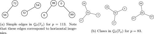
Examples of the first three of the four above are given by Figure 2. An example of attachment along a j-invariant can be seen in Figure 3. It can happen that an attachment is actually attaching the component V to itself. See Figure 4. We will show that attachment along the j-invariant for $\mathcal{l}=2$ cannot happen in Corollary 3.24, however, the j-invariant 1728 is the only possible j-invariant for which the two vertices in ${\mathcal{G}}_2({\mathbb{F}}_p)$ do not have the same neighbor set (Proposition 3.22), but in this case these vertices are already connected by an edge.

Fig. 1 The graph ${\mathcal{G}}_2({\mathbb{F}}_p)$ for p = 431 (case 3.a of Theorem 3.5). The vertices are labeled by j-invariants of each curve. Each component is a volcano, with an inner ring of surface curves and the outer vertices all being curves on the floor. The class number of $\mathbb{Q}\left(\sqrt{-431}\right)$ is $3·7=21$ and the orders of the two primes above 2 are 7.

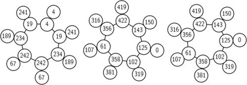
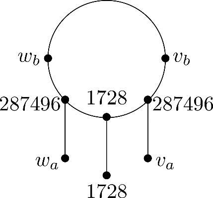
Fig. 2 Stacking, folding and attaching by an edge for p = 431 and $\mathcal{l}=2$. The leftmost component of ${\mathcal{G}}_2({\mathbb{F}}_p)$ folds, the other two components stack, and the vertices 189 and 150 get attached by a double edge.

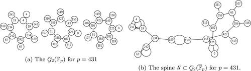
Fig. 3 Attachment along a j-invariant for p = 83 and $\mathcal{l}=3$. The two connected components of ${\mathcal{G}}_3({\mathbb{F}}_p)$ are attached along the j-invariant $68=1728\text{mod}83$. There are two outgoing double edges from j = 1728 but because of the extra automorphisms, these edges are identified in the undirected graph.

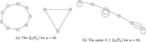
Fig. 4 Attachment by an edge that does not attach two distinct components. This component folds and the vertices with j-invariants 68 and 107 are joined by a double edge.

We now begin analyzing the ‘new’ edges in $\mathcal{S}$: the edges that do not come from isogenies defined over ${\mathbb{F}}_p$. For an elliptic curve E, all $\mathcal{l}$-isogenies are given by order $\mathcal{l}$ subgroups of the $\mathcal{l}$-torsion subgroup $E[\mathcal{l}]$. An $\mathcal{l}$-isogeny is defined over ${\mathbb{F}}_p$ if and only if its kernel is fixed by the Frobenius endomorphism. Note that this does not mean that all the points in the kernel need to be fixed by Frobenius.

Let us look at Figure 2 again: the edges in the spine $\mathcal{S}$ between vertices corresponding to j-invariants 150 and 189 in ${\mathcal{G}}_2({\overline{\mathbb{F}}}_p)$ do not correspond to isogenies defined over ${\mathbb{F}}_p$. Also, the vertex 4 (and note $4\equiv 1728\text{mod}431$) on the floor of ${\mathcal{G}}_2({\mathbb{F}}_p)$ has no edge to a curve with j-invariant 19, but there is an edge $[4,19]\in {\mathcal{G}}_2({\overline{\mathbb{F}}}_p)$ coming from the two isogenies from vertex 4 on the surface. Lemma 3.10 gives us that there is a double edge $[4,19]\in {\mathcal{G}}_2({\overline{\mathbb{F}}}_p)$. This not a coincidence, as we explain in Lemma 3.14.

Lemma 3.14

(One new isogeny implies two new isogenies). Let $v_a,v_b\in {\mathcal{G}}_{\mathcal{l}}({\mathbb{F}}_p)$ correspond to ${\mathbb{F}}_p$-elliptic curves E_a and E_b with j-invariants a, b respectively with $a\ne 1728,0$. Assume that there is no edge $[v_a,v_b]\in {\mathcal{G}}_{\mathcal{l}}({\mathbb{F}}_p)$, but there is an edge $[a,b]\in {\mathcal{G}}_{\mathcal{l}}({\overline{\mathbb{F}}}_p)$. Then there are two isogenies defined between $E_a\to E_b$ which are inequivalent over ${\overline{\mathbb{F}}}_p$ and hence a double edge $[a,b]\in {\mathcal{G}}_{\mathcal{l}}({\overline{\mathbb{F}}}_p)$.

Proof.

We know that there is an $\mathcal{l}$-isogeny $\varphi :E_a\to E$ to some elliptic curve E with j-invariant b. Since j(E) = b, then E is isomorphic to E_b over ${\mathbb{F}}_{p^2}$. Composing with this isomorphism, we obtain an $\mathcal{l}$-isogeny $\psi :E_a\to E_b$. However, ψ cannot be defined over ${\mathbb{F}}_p$, since we assumed there was no edge $[v_a,v_b]\in {\mathcal{G}}_{\mathcal{l}}({\mathbb{F}}_p)$.

The kernel of ψ is not defined over ${\mathbb{F}}_p$ (otherwise ψ would be defined over ${\mathbb{F}}_p$), so the p-power Frobenius map $\text{Frob}:{\mathbb{F}}_p\to {\mathbb{F}}_p$ does not preserve $\ker \psi$. There is an isogeny from E_a with kernel ${\psi }^{\text{Frob}}$. This isogeny has degree $\mathcal{l}$ since ${\psi }^{\text{Frob}}$ has order $\mathcal{l}$ and it is not equivalent to ψ. Using the construction of isogenies from Vélu’s formulae [27], we obtain the rational maps for defining ${\psi }^{\text{Frob}}$. In particular, the j-invariant of the target of ${\psi }^{\text{Frob}}$ is necessarily $\text{Frob}(b)=b$. Hence, there are two inequivalent isogenies between E_a and E_b and hence two edges $[a,b]\in {\mathcal{G}}_{\mathcal{l}}({\overline{\mathbb{F}}}_p)$. □

The corollary below explains why for both attachment by a new edge (cf. Figures 2 and 4) and attachment along a j-invariant (cf. Figure 3), we always see double edges.

Corollary 3.15.

Attachment of components by a new edge from v_a to w_b forces a double edge $[a,b]$ in ${\mathcal{G}}_{\mathcal{l}}({\overline{\mathbb{F}}}_p)$. Attachment along the j-invariant j implies a double edge from j in ${\mathcal{G}}_{\mathcal{l}}({\overline{\mathbb{F}}}_p)$.

Proof.

In the first case, we are adding an edge between v_a and w_b that is not defined over ${\mathbb{F}}_p$ and we can directly apply Lemma 3.14. In the second case, assume there is a neighbor v_b of $v_{\mathbf{j}}$ such that w_b is not a neighbor of $w_{\mathbf{j}}$. Apply the Lemma 3.14 to the ${\overline{\mathbb{F}}}_p$ isogeny from $w_{\mathbf{j}}$ to v_b. □

Because we take the isogeny graphs undirected, we need to make choices at $\mathbf{j}=1728$ or $\mathbf{j}=0$. In this case, double edges might get identified because of the choices for the undirectedness of the graph.

3.3 The spine for $\mathcal{l}>2$

For this section, we consider the spine $\mathcal{S}$ for $\mathcal{l}>2$. In this case, there are no vertical isogenies, hence the graph ${\mathcal{G}}_{\mathcal{l}}({\mathbb{F}}_p)$ is a union of disjoint cycles: the cycles of vertices corresponding to curves either only with endomorphism ring $\mathbb{Z}\left[\frac{1+\sqrt{-p}}{2}\right]$, or only with endomorphism ring $\mathbb{Z}[\sqrt{-p}]$. The main tool for understanding the spine will be the Neighbor Lemma 3.17, in which we show that the vertices v_a and w_a have neighbors with the same j-invariants, provided $a\ne 1728$. If the neighbors have different j-invariants, then we would get attachment along a vertex and this situation we solve in Proposition 3.16. Using the information about the shape of the graph ${\mathcal{G}}_{\mathcal{l}}({\mathbb{F}}_p)$ and the neighbor lemma, we can completely describe the spine $\mathcal{S}$ in Theorem 3.18.

We will avoid the case when the graph ${\mathcal{G}}_{\mathcal{l}}({\mathbb{F}}_p)$ is just a disjoint union of vertices (i.e., when there are no isogenies defined over ${\mathbb{F}}_p$) by assuming $\mathcal{l}$ is split in $\mathbb{Z}[\sqrt{-p}]$. If one assumes that $p\equiv -1\text{mod}\mathcal{l}$, then $\mathcal{l}|\#E({\mathbb{F}}_p)=p+1$ and there are ${\mathbb{F}}_p$-rational points of order $\mathcal{l}$. We will also assume that the class number $\text{cl}(\mathbb{Z}[\sqrt{-p}])$ is odd, which is equivalent to $p\equiv 3\mathrm{mod}4$.

Proposition 3.16

(Attachment along a vertex can only happen at a vertex with automorphisms). Let p and $\mathcal{l}$ be primes satisfying ${\mathcal{l}}^4<\frac{1}{4}p$. Let j be a j-invariant such that attachment along a vertex happens. Then $\mathbf{j}=1728$, the two neighbors in ${\mathcal{G}}_{\mathcal{l}}({\mathbb{F}}_p)$ of v₁₇₂₈ have the same j-invariant and the neighbors of w₁₇₂₈ have the same j-invariant.

The proof below uses the properties of the ${\overline{\mathbb{F}}}_p$-endomorphism ring $\text{End}(E)$ as a maximal order in a quaternion algebra. For references see Kohel’s thesis [19], the work of Kaneko [17] and Ibukiyama [16].

Proof.

We first show that j corresponds to an elliptic curve with automorphism group larger than $\{\pm 1\}$, so $\mathbf{j}=1728$ or 0. Then, we show that $\mathbf{j}=0$ cannot happen.

Let E be a supersingular elliptic curve and let $\text{End}(E)$ be its endomorphism ring. Recall that $\text{End}(E)$ is a maximal order in a quaternion algebra. Every element $\alpha \in \text{End}(E)\setminus \mathbb{Q}$ is quadratic, meaning α generates a quadratic number field $\mathbb{Q}(\alpha )$.

From Kaneko’s Theorem 2’ [17], we know that If $O,O\prime$ are maximal quadratic orders lying in different imaginary quadratic fields that embed to $\text{End}(E)$ then $\text{disc}(O)·\text{disc}(O\prime )\ge 4p.$

Suppose now that we have attachment at a vertex j. Let v_a, v_b be the neighbors of $v_{\mathbf{j}}$ and let w_c, w_d be the neighbors of $w_{\mathbf{j}}$, with $a\notin \{c,d\}$. Then, by Corollary 3.15, there is a double edge from $[a,\mathbf{j}]\in {\mathcal{G}}_{\mathcal{l}}({\overline{\mathbb{F}}}_p)$ and, by symmetry, there is a double edge from either c or d, assume without loss of generality that it is from c. Any double edge gives a non-trivial element of norm ${\mathcal{l}}^2$ in $\text{End}(E)$. Let α denote the cycle arising from the double edge at a, and γ the cycle arising from the double edge at c.

Suppose that α and γ generate different quadratic number fields. Then, we observe that$${\mathcal{l}}^2=\text{nrd}(\alpha )\ge \frac{1}{4}\text{disc}(\mathbb{Z})\left[\alpha \right]\ge \frac{1}{4}\text{disc}(\mathbb{Q}(\alpha ))$$and we obtain a similar statement for γ. Using Kaneko’s theorem we deduce that$${\mathcal{l}}^2·{\mathcal{l}}^2=\text{nrd}(\alpha )·\text{nrd}(\beta )\ge \frac{1}{16}\text{disc}(\mathbb{Q}(\alpha ))·\text{disc}(\mathbb{Q}(\gamma ))\ge \frac{1}{4}p,$$ which is impossible for ${\mathcal{l}}^4<\frac{1}{4}p$. We conclude that α and γ generate the same quadratic field, say K. Let ${\mathcal{O}}_K$ be the ring of integers in K. By uniqueness of ideal factorization:$$(\alpha )(\overline{\alpha })=({\mathcal{l}}^2)=(\gamma )(\overline{\gamma })={(\mathcal{l})}^2=\{\begin{array}{cc}{(\mathcal{l})}^2\hfill & \text{if}\mathrm{}\mathcal{l}\mathrm{}\text{is}\mathrm{}\text{inert},\hfill \\ {\mathfrak{l}}^4\hfill & \text{if}\mathrm{}\mathcal{l}\mathrm{}\text{is}\mathrm{}\text{ramified},\hfill \\ {(\mathfrak{l}\overline{\mathfrak{l}})}^2\hfill & \text{if}\mathrm{}\mathcal{l}\text{splits}.\hfill \end{array}$$

Since $\alpha \notin \mathbb{Q},\mathcal{l}$ cannot be inert. If $\mathcal{l}$ is ramified, we see:$$(\alpha )=(\gamma )={\mathfrak{l}}^2\to \alpha =u\gamma$$for some unit $u\in {\mathcal{O}}_K$. It is not possible that $\alpha =\pm \gamma$, so $\{\pm 1\}⊊\text{Aut}(E)$.

If $\mathcal{l}$ splits, suppose without loss of generality that $(\alpha )={\mathfrak{l}}^2$. Then either$$\begin{array}{c}(\gamma )={\mathfrak{l}}^2\to \gamma =u·\alpha \\ \text{or}(\gamma )={\overline{\mathfrak{l}}}^2\to \overline{\gamma }=u·\alpha \end{array}$$for some unit $u\in {\mathcal{O}}_K$. Again implies that ${\mathcal{O}}_K$ has non-trivial units and $\{\pm 1\}⊊\text{Aut}(E)$.

Curves with automorphism group larger than $\{\pm 1\}$ correspond to $\mathbf{j}=0,1728$. Suppose $j(E_0)=0$. If there is an isogeny from an elliptic curve E₀ to an elliptic curve E_a with j-invariant a, there have to be at least three distinct isogenies from E₀ to E_a: precompose the first one with ${\zeta }_3,{\zeta }_3^2\in \text{End}(E_0)$. However, suppose that there were three edges from 0 to a. By symmetry, there would be three edges from 0 to c in ${\mathcal{G}}_{\mathcal{l}}({\overline{\mathbb{F}}}_p)$. By combining these edges, we would have 6 cycles from 0 of length 2. But even in $\mathbb{Z}[{\zeta }_3]$, up to sign (±), there are not enough different elements of norm ${\mathcal{l}}^2$.

Hence attachment along a vertex can only happen for $\mathbf{j}=1728$. □

Lemma 3.17

(The neighbor lemma). Suppose $\mathcal{l}>2$. Let $a\ne 1728$ and suppose that v_a, w_a are the two vertices in ${\mathcal{G}}_{\mathcal{l}}({\mathbb{F}}_p)$ corresponding to elliptic curves with j-invariant a. If the neighbors of v_a have j-invariants b, c, then then neighbors of w_a have j-invariants b, c.

Proof.

Let w_d, w_e be the neighbors of w_a in ${\mathcal{G}}_{\mathcal{l}}({\mathbb{F}}_p)$. If $\{d,e\}\ne \{b,c\}$, then there is attachment along the j-invariant a, which is only possible for $\mathbf{j}=1728$. Hence the neighbors of v_a and w_a have the same j-invariants. □

Recall that the attachment of components by a new edge implies a double edge by Corollary 3.15. The main result of this section is the following one.

Theorem 3.18

(Stacking, folding and attaching for $\mathcal{l}>2$). Let p be a prime and let $\mathcal{l}$ be such that the order of the prime $\mathfrak{l}$ above $\mathcal{l}$ in the class group $\text{cl}(-p)$ of $\mathbb{Q}\left(\sqrt{-p}\right)$ is odd. While passing from ${\mathcal{G}}_{\mathcal{l}}({\mathbb{F}}_p)$ to $\mathcal{S}$, the following happens:

1. the components containing 1728 fold and get attached along the j-invariant 1728 (this only happens if $p\equiv 3\text{mod}4$),

2. all other components stack,

3. the number of new edges is bounded by $\mathrm{deg}Re{s}_{\mathcal{l}}(X)$ and there are at most n vertices at which a new edge is added, where n is the number of distinct roots of $Re{s}_{\mathcal{l}}(X)$.

Note that the conditions on p and $\mathcal{l}$ are always satisfied when $p\equiv 3\text{mod}4$ and $p\equiv -1\text{mod}\mathcal{l}$, which is the most cryptographically relevant application.

Proof.

We will pass from ${\mathcal{G}}_{\mathcal{l}}({\mathbb{F}}_p)$ to $\mathcal{S}$ in two steps: first, we identify the j-invariants and equivalent edges in ${\mathcal{G}}_{\mathcal{l}}({\mathbb{F}}_p)$, and after discussing what happens with the components of ${\mathcal{G}}_{\mathcal{l}}({\mathbb{F}}_p)$, we add the new edges in ${\mathcal{G}}_{\mathcal{l}}({\overline{\mathbb{F}}}_p)$.

We showed in Lemma 3.17 that for $a\ne 1728$, the vertices v_a and w_a have the same neighbors.

Suppose there is a component V that does not stack. This either means that there is a vertex v_a whose neighbors are different than those of w_a. But in this case a is an attaching j-invariant and so a = 1728 and we will treat this case later.

Or, there is a j-invariant a such that both the vertices v_a, w_a are in the component V. We know that V is a cycle with odd number of vertices. The vertices v_a, w_a divide the cycle in two halves. Choose either half H. Look at the neighbors of v_a and w_a. If they have the same j-invariant b, replace a with b and continue moving along the halves of the cycle, until either of the following happens:

1. the vertices v_a and w_a are neighbors in ${\mathcal{G}}_{\mathcal{l}}({\mathbb{F}}_p)$ and hence will induce a loop in ${\mathcal{G}}_{\mathcal{l}}({\overline{\mathbb{F}}}_p)$. Note that in this case, the number of vertices in H is necessarily even.

2. The only neighbor of v_a and w_a is a vertex v_j with j-invariant j. This is necessarily an attaching j-invariant because the neighbors of w_j cannot have j-invariants a. Hence $\mathbf{j}=1728$. This also means that H has an odd number of vertices.

3. The neighbor v_b of v_a has j-invariant b and the neighbor w_c of w_a has j-invariant c, for $b\ne c$. Then either the other neighbor of w_a is w_b or a is an attaching j-invariant (and a = 1728). Suppose a is not an attaching j-invariant. Continuing along the whole cycle V in the direction of the edge $[v_a,v_b]$, and symmetrically in the direction of $[w_a,w_b]$, we will reach a point when the neighbor of some v_c is not a neighbor of the w_c. This happens when the cycle has an odd number of vertices because two identical paths would give us a cycle of even length. Here we also obtain an attaching j-invariant.

The cases above actually cover every possibility: if we are in case (3.3), the half H has an even number of vertices, and then $V\setminus H\cup \{v_a,w_a\}$ necessarily has an odd number of vertices and since the neighbors of v_a, w_a have to have the same j-invariant, we are in case (3.3).

Let us remark that the last case (3.3) shows that the isogenies between twists go ‘in the other direction’: if one walks on the cycle V in the direction of the edge $[v_a,v_b]$, one will encounter an edge $[w_b,w_a]$, not an edge $[w_a,w_b]$.

We now discuss what happens with the components that contain 1728. We know that there are two components V and W containing curves with j-invariant 1728. Let $v_a\in V$ be on the surface (with curves having ${\text{End}}_{{\mathbb{F}}_p}(E)\cong {\mathcal{O}}_K$) and let $w_a\in W$ be on the floor (with curves having ${\text{End}}_{{\mathbb{F}}_p}(E)\cong \mathbb{Z}[\sqrt{-p}]$). We have shown in 3.16 that both v₁₇₂₈ and w₁₇₂₈ have two neighbors neighbors with the same j-invariant. We will show that both the components fold.

Starting at the vertex $v_{1728}\in V$, we know that its neighbors v_a, w_a have the same j-invariant by Lemma 3.16. Start walking away from v₁₇₂₈. By the Neighbor Lemma 3.17, the neighbors of the vertices v_a, w_a that are different from v₁₇₂₈ have the same j-invariants. Continuing this reasoning, since the cycle contains an odd number of vertices, one finally arrives at a pair of vertices v_b, w_b with same j-invariant b, which are connected by an $\mathcal{l}$-isogeny. The same proofs holds for the component W containing w₁₇₂₈.

Finally, adding new edges that are only defined over ${\overline{\mathbb{F}}}_p$, some components can get attached. However, we have proved in Corollary 3.15 that an attachment by a new edge from j to double $\mathbf{j}\prime$ means a double edge $[\mathbf{j},\mathbf{j}\prime ]\in {\mathcal{G}}_{\mathcal{l}}({\overline{\mathbb{F}}}_p)$. Hence j and $\mathbf{j}\prime$ are both roots of ${\text{Res}}_{\mathcal{l}}(X)$ by Lemma 2.7, which has degree bounded by $2\mathcal{l}·(2\mathcal{l}-1)$. □

Remark 3.19

(The ‘other side’ of 1728). We showed that the only component for which attachment by a vertex can happen are the two components containing 1728, moreover these components fold. This means that the neighbors of v₁₇₂₈ have the same j-invariant, their neighbors as well and if we continue walking along both sides, we will ultimately meet ‘opposite of’ v₁₇₂₈ at a pair of conjugate j-invariants. See Figure 4(a). Conversely, any such pair of conjugate j-invariants needs to be ‘opposite’ of a vertex with j-invariant 1728.

Since posting the first version of our article which did not fully explain these ideas, Castryck, Panny and Vercauteren posted a preprint [10] that arrives at the same conclusion using more highbrow tools. Their approach identifies the ‘opposite’ j-invariant as a certain CM j-invariant.

As noted Corollary 3.15, attachments imply double edges. To find vertices with attachment, we can use Lemma 2.7. Conversely, if we want a prime p with no attachments, we can find a congruence condition on p such that none of the roots if ${\text{Res}}_{\mathcal{l}}(X)$ are supersingular j-invariants.

3.3.1 Example: the spine for $\mathcal{l}=3$

In this section, we decsribe the spine $\mathcal{S}$ for $\mathcal{l}=3$ by means of stacking, folding and attaching behavior for $\mathcal{l}=3$. The case $\mathcal{l}=3$ is interesting, because of the use of ${\mathcal{G}}_3({\overline{\mathbb{F}}}_p)$ in SIDH and SIKE (and analogously, the case $\mathcal{l}=2$ will be discussed in Section 3.4). Since the starting vertex for these protocols is typically taken in ${\mathbb{F}}_p$, understanding the spine is important for understanding where the ${\mathbb{F}}_p$ j-invariants are located in the graph ${\overline{\mathbb{F}}}_p$.

We start with factoring over $\mathbb{Z}$ the polynomial ${\text{Res}}_3(x)$ introduced in (3):$$\begin{array}{c}{\text{Res}}_3(x)=\left(-1\right)·3^3·x^2·{(x-8000)}^2·{(x-1728)}^2·{(x+32768)}^2\\ ·{(x^2-52250000x+12167000000)}^2·{(x^2-1264000x-681472000)}^2\\ ·{(x^2+117964800x-134217728000)}^2.\end{array}$$

The irreducible factors are Hilbert class polynomials of discriminants $-3,-8,-4,$ $-11,-32,-20$ and –35, respectively. Removing the repeated factors, we see that there are at most 10 vertices at which a double edge can occur.

Double-edges also arise in loops (double self-3-isogenies), which accounts for some of the factors of ${\text{Res}}_3(x)$. We find the self loops by factoring the modular 3-isogeny polynomial:$${\Phi }_3(x,x)=\left(-1\right)·x·(x-54000)·{(x-8000)}^2·{(x+32768)}^2.$$

At $\mathbf{j}=8000$ and $\mathbf{j}=-32768$, there are two self-3-isogenies and no attachment at these vertices.

Example 3.20

(Vertices with loops). In this example, we determine the ${\mathcal{G}}_3({\mathbb{F}}_p)$ neighbors of $\mathbf{j}=0,8000,54000$ and –32768. This is done by factoring ${\Phi }_3(\mathbf{j},x)$:

1. $\mathbf{j}=0$: Factor ${\Phi }_3(0,x)={(x+12288000)}^3·x$. The isogeny v₀, w₀ is defined over ${\mathbb{F}}_p$: the factor x has multiplicity 1, so it is not a double-edge and cannot appear only over ${\mathbb{F}}_{p^2}$. Moreover, the neighbors of v₀ are w₀ and $v_{-12288000}$ and the neighbors of w₀ are $w_{-12288000}$ and v₀. Hence there cannot be attaching edges.

2. $\mathbf{j}=54000$: There is one self-3-isogeny which arises from a 3-isogeny ψ between (non-isomorphic) quadratic twists with j = 54000 and that can be written explicitly. Factoring ${\varphi }_3(54000,x)$ we can check that the j-invariant 54000 does not admit a double edge.

3. $\mathbf{j}=8000$: we have ${(x-8000)}^2|{\Phi }_3(8000,x)$ and so there is a double loop $[8000,8000]\in {\mathcal{G}}_3({\overline{\mathbb{F}}}_p)$. Neither of the loops occur over ${\mathbb{F}}_p$: both cannot occur over ${\mathbb{F}}_p$ because there are no double edges in ${\mathcal{G}}_3({\mathbb{F}}_p)$. If only one of them came from an isogeny over ${\mathbb{F}}_p$, then we could use Lemma 3.14 to get a third loop, which is not possible (for large p).

4. $\mathbf{j}=-32768$: again, ${(x+32768)}^2|{\Phi }_3(-32768,x)$. Repeating the argument we gave above for $\mathbf{j}=8000$, the self loops cannot come from isogenies over ${\mathbb{F}}_p$.

To conclude: For $\mathbf{j}=0$ and 54000, the self-3-isogeny comes from an isogeny between the twists in ${\mathcal{G}}_3({\mathbb{F}}_p)$, and for $\mathbf{j}=8000,-32768$, the double self-3-isogenies are not defined over ${\mathbb{F}}_p$.

The following theorem is a specialization of Proposition 3.18. We are mainly interested in the cryptographic applications, so we restrict to the case $p\equiv 3\text{mod}4$. Then, the class numbers $h(-p)$ and $h(-4p)=3·h(-p)$ are both odd. With our assumption $p\equiv 2\text{mod}3$, we have $p\equiv 11\text{mod}12$.

Theorem 3.21

(Stacking, folding and attaching for $\mathcal{l}=3$). Let p be prime, $p\equiv 11\text{mod}12$. When passing from ${\mathcal{G}}_3({\mathbb{F}}_p)$ to the spine $\mathcal{S}\subset {\mathcal{G}}_3({\overline{\mathbb{F}}}_p)$,

1. all components that do not contain 0 or 54000 stack,

2. there are two distinct connected components V and W that contain a j-invariant 1728, one of them contains both vertices with j-invariant 0 and the other one both vertices with j-invariant 54000. V and W fold and get attached at the j-invariant 1728.

3. At most 8 vertices admit new edges, attaching at most 4 pairs of components by a new edge.

Proof.

This follows from Theorem 3.18. In Example 3.20, we showed that the only possible opposite vertices have j-invariants 0 and 54000. For $p\equiv 3\text{mod}4$, there are two components containing 1728: by Example 3.8, one of the vertices corresponding to 1728 is on the floor and the other one is on the surface, so they are on different components of ${\mathcal{G}}_3({\mathbb{F}}_p)$. One of these vertices is on the same component of ${\mathcal{G}}_3({\mathbb{F}}_p)$ as the vertices with j-invariant 0 and the other one will contain both vertices with j-invariant 54000. The rest comes from looking at the factors of ${\text{Res}}_3(x)$. □

3.4 The spine for $\mathcal{l}=2$

In this section, we describe the spine $\mathcal{S}$ for $\mathcal{l}=2$. The added difficulty are vertical isogenies (see Definition 3.4). We describe how the components of ${\mathcal{G}}_2({\mathbb{F}}_p)$ come together in $\mathcal{S}\subset {\mathcal{G}}_2({\overline{\mathbb{F}}}_p)$ in a way analogous to $\mathcal{l}>2$ (see Theorem 3.29). We determine whether attachment can happen for $p\equiv 1\text{mod}4$ and $p\equiv 3\text{mod}8$ (see Corollary 3.30) and we give experimental data on $p\equiv 7\text{mod}8$.

Delfs and Galbraith [11] described the possible shapes for ${\mathcal{G}}_2({\mathbb{F}}_p)$, which we will extensively use in this section:

Table

Residue class of p	Endomorphism rings	Shape of ${\mathcal{G}}_2({\mathbb{F}}_p)$
$p\equiv 1\text{mod}4$	$\mathbb{Z}[\sqrt{-p}]$	Each connected component is two vertices connected by one edge, corresponding to a horizontal isogeny (see Figure 6(a)).
$p\equiv 3\text{mod}8$	$\mathbb{Z}[\sqrt{-p}],\mathbb{Z}\left[\frac{1+\sqrt{-p}}{2}\right]$	Each connected component is “claw”: one vertex on the surface connected to three vertices on the floor by vertical isogenies (see Figure 6(b).)
$p\equiv 7\text{mod}8$	$\mathbb{Z}[\sqrt{-p}],\mathbb{Z}\left[\frac{1+\sqrt{-p}}{2}\right]$	Each connected component is a 2-level “volcano” with surface a cycle of size $\ge 1$. From any vertex on the surface there is exactly one vertical isogeny. There are no horizontal isogenies on the floor (see Figure 1.)

Recall that we form the graph $\mathcal{S}$ from ${\mathcal{G}}_2({\mathbb{F}}_p)$ in two steps: first merge vertices corresponding to the same j-invariant and their edges, then add new edges. We will show that:

1. Two vertices with the same j-invariant also have the same j-invariants as neighbors (Proposition 3.22). This will imply that only stacking and folding is possible in Theorem 3.29.

2. At most one component folds, and for $p\equiv 3\text{mod}4$ this is the component containing $\mathbf{j}=1728$ (Proposition 3.26).

3. Attaching of components by a new edge happens between at most one pair of vertices, and those vertices are roots of the Hilbert class polynomial of $\mathbb{Q}\left(\sqrt{-15}\right)$ (Proposition 3.25).

We begin with some results on the neighbors of vertices with the same j-invariant. From Corollary 3.7, we know that (except for 1728) twists have isomorphic endomorphism rings and hence lie on the same level in the volcano. More is true:

Proposition 3.22.

Let j be a supersingular j-invariant and let $v_{\mathbf{j}}$ and $w_{\mathbf{j}}$ be two distinct vertices in ${\mathcal{G}}_2({\mathbb{F}}_p)$ corresponding to elliptic curves with j-invariant j. If $\mathbf{j}\ne 1728$, then two vertices with the same j-invariants have the same neighbors, that is:

1. If $p\equiv 1\text{mod}4$ and the neighbor of $v_{\mathbf{j}}$ is $v_{\mathbf{j}\prime }$, then the neighbor of $w_{\mathbf{j}}$ is $w_{\mathbf{j}\prime }$.

2. If $p\equiv 3\text{mod}4$ and if

   1. the vertices $v_{\mathbf{j}}$ and $w_{\mathbf{j}}$ are both on the floor, then $v_{\mathbf{j}}$ and $w_{\mathbf{j}}$ are each connected to a vertex with j-invariant $\mathbf{j}\prime$,

   2. the vertices $v_{\mathbf{j}}$ and $w_{\mathbf{j}}$ are both on the surface, then $v_{\mathbf{j}}$ has 3 neighbors with distinct j-invariants a, b, c and $w_{\mathbf{j}}$ has three neighbors with the same distinct j-invariants a, b, c.

Proof.

1. For $p\equiv 1\text{mod}4$, any connected component of ${\mathcal{G}}_2({\mathbb{F}}_p)$ is an edge. If $v_{\mathbf{j}}$ and $w_{\mathbf{j}}$ lie on the same component, then the result follows. Otherwise, the result can be obtained by contradiction and an application of Lemma 3.14.

2. If $p\equiv 3\text{mod}4$, Corollary 3.9 gives $v_{\mathbf{j}},w_{\mathbf{j}}$ are either both on the surface and on the floor of their respective components.

If they are both on the surfaces of their respective components, then they each have three neighbors: one on the floor and two on the surface. The j-invariants of the neighbors of $v_{\mathbf{j}}$ match the j-invariants of the neighbors of $w_{\mathbf{j}}$. Any coincidences of these j-invariants would contradict the fact that there can be no cycles of length 2: for $p\equiv 3\text{mod}4$, the class number $h(-p)$ is odd.

If they are both on the floors of their respective components, then they each have one neighbor on the surface. The j-invariants of these neighbors must be the same, otherwise we arrive at a contradiction via Lemma 3.14 as in 1.

Corollary 3.23

(Isogenies for twists). Let $\varphi :E\to E\prime$ be an ${\mathbb{F}}_p$-isogeny of degree 2 and assume $j(E),j(E\prime )\ne 1728$. Then, there is an 2-isogeny over ${\mathbb{F}}_p$ between the quadratic twists $E^t\to {(E\prime )}^t$.

Corollary 3.24

(Attachment along a j-invariant for $\mathcal{l}=2$). Attachment along a j-invariant cannot happen for $\mathcal{l}=2$.

We already know that attaching two components by a new edge would imply a double edge (Corollary 3.15).

Proposition 3.25

(Possible attachment by a double edge). Attachment by an edge can only happen between vertices whose j-invariants correspond to the roots of $$f(X)=X^2+191025X-121287375$$

in ${\mathbb{F}}_p$, provided these are supersingular ${\mathbb{F}}_p$ j-invariants not equal to $-3375,1728$ or 0.

Proof.

By Lemma 2.7 and Corollary 3.15, any such attaching j-invariants need to be roots of ${\text{Res}}_2(X)$. By examining the neighbors of the j-invariants 0, 1728 and –3375, we can easily see that they do not admit new edges coming from isogenies not defined over ${\mathbb{F}}_p$. □

Proposition 3.26

(The component of $\mathbf{j}=1728$ folds). Let $p\equiv 3\text{mod}4$ be prime. The connected component $V\in {\mathcal{G}}_2({\mathbb{F}}_p)$ containing the vertices corresponding to $\mathbf{j}=1728$ is symmetric over a reflection passing through the vertices v₁₇₂₈ lying on the surface of V and w₁₇₂₈ lying on the floor of V. In particular, the component V folds when we pass from ${\mathcal{G}}_2({\mathbb{F}}_p)$ to $\mathcal{S}$.

To understand this symmetry, picture the surface of the component V as a perfect circle with equidistant vertices and all the edges to the floor are perpendicular to the surface. Then V is symmetric with respect to the line extending the edge $[v_{1728},w_{1728}]$. See the leftmost component in Figure 1. This symmetry has already mentioned in Remark 5 of [8], albeit without proof or reference.

Proof.

1. Case $p\equiv 3\text{mod}8$. V is a claw (see Figure 6(a)) and the proof of Proposition 3.25 shows that there is one 2-isogeny down from the surface vertex corresponding to $\mathbf{j}=1728$ to each vertex with j-invariant 287496 and the other vertex corresponding to j-invariant 1728. The claw V is clearly symmetric and folds as described.

2. Case $p\equiv 7\text{mod}8$. In this case, $h(-p)$ is odd. We may assume that $h(-p)>1$ (otherwise we are in the claw situation discussed above).

Fig. 5 The graph ${\mathcal{G}}_3({\mathbb{F}}_p)$ for p = 179. We see that the neighbors of vertices with j-invariant 0 both have j-invariant $-12288000\text{mod}179=171$.

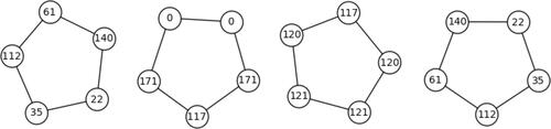
Fig. 6 Possible shapes for ${\mathcal{G}}_2({\mathbb{F}}_p)$ for $p\equiv 1\text{mod}4$ (left) and $p\equiv 3\text{mod}8$.

Then $v=v_{287,496}$ and $w=v_{287,496}^t$ are both on the surface. By Proposition 3.22, their neighbors have the same j-invariants, say: $1728,a,b$. Say the neighbors of v are v_a, v_b and the neighbors of w are w_a, w_b. Assume that v_a is on the floor. Since $a\ne 1728$, Lemma 3.9 tells us w_a is also on the floor. Thus, both v_b and w_b are on the surface and the symmetry is preserved.

Continuing in this manner, because $h(-p)$ is odd, we will arrive at a pair of vertices $v_{\mathbf{c}},w_{\mathbf{c}}$ that share an edge, accounting for all of the vertices in the component. The symmetry holds. □

Remark 3.27.

In Proposition 3.26 for $p\equiv 7\text{mod}8$, the opposite vertices $v_{\mathbf{c}},w_{\mathbf{c}}$ from j = 1728 necessarily induce a loop in ${\mathcal{G}}_2({\overline{\mathbb{F}}}_p)$. Since $v_{\mathbf{c}},w_{\mathbf{c}}$ are on the surface of ${\mathcal{G}}_2({\mathbb{F}}_p)$, we conclude that $\mathbf{c}=8000$ (see Section 2.2). So there always is an ${\mathbb{F}}_p$-rational 2-power isogeny between any two supersingular elliptic curves with j-invariants 1728 and 8000.

Corollary 3.28

(Folding). Suppose $V\subset {\mathcal{G}}_2({\mathbb{F}}_p)$ is a component which folds when passing from ${\mathcal{G}}_2({\mathbb{F}}_p)$ to $\mathcal{S}\subset {\mathcal{G}}_2({\overline{\mathbb{F}}}_p)$.

1. If $p\equiv 1\text{mod}4$, then V is a single edge between vertices with j = 8000.

2. If $p\equiv 3\text{mod}4$, then V contains both the vertices corresponding to $\mathbf{j}=1728$.

Proof.

1. If $p\equiv 1\text{mod}4$, then V is an edge: $[v_a,v_b]$. Folding happens if and only if a = b, resulting in a self-2-isogeny in ${\mathcal{G}}_{\mathcal{l}}({\overline{\mathbb{F}}}_p)$. For $p\equiv 1\text{mod}4$, the only vertices with self-2-isogenies are $\mathbf{j}=-3375,8000$, when these j-invariants are supersingular (see Section 2.2).

   For j = 8000, there is a 2-isogeny from the curve with j-invariant 8000 given by the equation $E:y^2=x^3-4320x-96768$ to its twist $y^2=x^3-17280x-774144$. The latter is a twist of E by 2, and 8000 is only supersingular for $p\equiv 5\text{mod}8$, so 2 is a nonsquare modulo p.

   For $\mathbf{j}=-3375$, there are two self-loops in ${\mathcal{G}}_2({\overline{\mathbb{F}}}_p)$, and at least one of them is not defined over ${\mathbb{F}}_p$. Applying Lemma 3.14 to this loop, we conclude that neither of these loops are defined over ${\mathbb{F}}_p$ and folding does not happen for the edge containing –3375.

2. If $p\equiv 3\text{mod}4$, then let V be a component that folds. The surface has $h(-p)$ vertices and this class number is odd. We assume that V folds, so every vertex in it gets identified with the vertex corresponding to its twist. By Corollary 3.9, for $\mathbf{j}\ne 1728$, the two vertices are either both on the surface or both on the floor. Since there are odd number of vertices on the surface, there cannot only be pairs of twists on the surface, so V must contain the two vertices corresponding to $\mathbf{j}=1728$, one on the floor and the other on the surface. □

We are now ready to prove the main theorem describing the spine $\mathcal{S}$:

Theorem 3.29

(Stacking, folding and attaching). Only stacking, folding or at most 1 attachment by a new edge are possible. No attachments at a j-invariant are possible.

Proof.

First, let $p\equiv 1\text{mod}4$. The components of ${\mathcal{G}}_2({\mathbb{F}}_p)$ are edges. Corollary 3.28 shows that the edge containing the two vertices with j-invariant 8000 folds (if 8000 is a supersingular j-invariant for p, i.e., $p\equiv 5\text{mod}8$). For the other edges, Proposition 3.22 says that for any edge $[v_a,v_b]\in {\mathcal{G}}_2({\mathbb{F}}_p)$ the twists w_a, w_b also give an edge $[w_a,w_b]\in {\mathcal{G}}_2({\mathbb{F}}_p)$. Moreover, Proposition 3.25 gives that there is at most 1 attachment among these edges.

For $p\equiv 3\text{mod}4$, take any component V of ${\mathcal{G}}_2({\mathbb{F}}_p)$ and any vertex v_a on the surface of V, $a\ne 1728$. Choose a neighbor v_b of v_a. Continue along the surface in the direction of the edge $[v_a,v_b]$ and consider the sequence j-invariants of neighbors $\mathcal{V}=\left\{a_i\right\}$ until we reach a vertex with j-invariant a. Similarly, on the component W containing the edge w_a, w_b, consider the sequence of j-invariants of the neighbors $\mathcal{W}=\left\{b_i\right\}$ until we reach a vertex with j-invariant a (every surface is a cycle, so this will happen in finitely many steps). We have the following possible outcomes:

1. For some i, we find that $a_i\ne b_i$. This means that the curve i away from v_a on V has a different neighbor than its twist, which is i away from w_a. But this can only happen for b_i = 1728 and hence the component folds by Proposition 3.26.

2. The sequences are equal, but $\mathcal{V}$ stops at the twist w_a and $\mathcal{W}$ stopped at the curve v_a. Then v_a, w_a are on the same component V and the cycle on the surface has length $2·\text{length}(\mathcal{V})$. As $h(-p)$ is odd, this is not possible.

3. The sequences $\mathcal{V}$ and $\mathcal{W}$ are the same: the components V and W are isomorphic as graphs upon replacing the labels of vertices by their j-invariants. The components V and W stack.

Finally, in Proposition 3.25, we showed that at most one attachment is possible. □

To conclude this section, we study the possible attachments given by the roots of the polynomial $f(X)=X^2+191025X-121287375$. Because the polynomial f(X) is the Hilbert class polynomial of $\mathbb{Q}\left(\sqrt{-15}\right)$, roots of f(X) in ${\overline{\mathbb{F}}}_p$ give a supersingular j-invariant if and only if $\left(\frac{-15}{p}\right)=-1$. By factoring the discriminant of f(X) as $3^6·5^3·7^4·{13}^2,$ we see that there is a root in ${\mathbb{F}}_p$ if and only if $p\equiv \pm 1\text{mod}5$. Combining these, we obtain that the roots of f(X) are j-invariants of a supersingular elliptic curves defined over ${\mathbb{F}}_p$ if and only if $p\equiv 1,11,24$ or $59\text{mod}60$.

We have an additional result about when attachment occurs, as a corollary to Proposition 3.25:

Corollary 3.30

(Attachment happens for $p\cancel{\equiv }7\text{mod}8$). Suppose that $p\cancel{\equiv }7\text{mod}8$ and suppose that j and $\mathbf{j}\prime$ are two distinct ${\mathbb{F}}_p$-roots of $f(X)=X^2+191025X-121287375$ (it suffices to assume p > 101). Then, the new edge $[\mathbf{j},\mathbf{j}\prime ]\in {\mathcal{G}}_{\mathcal{l}}({\overline{\mathbb{F}}}_p)$ is an attaching edge.

This means that attachment happens whenever it can happen (i.e., when the roots of f(X) are in ${\mathbb{F}}_p$) for $p\cancel{\equiv }7\text{mod}8$. This is not true for $p\equiv 7\text{mod}8$ (See Section 3.5).

Proof.

First, let $p\equiv 1\text{mod}4$. The ${\mathcal{G}}_2({\mathbb{F}}_p)$ components are horizontal edges. Suppose that the j-invariant j admits a double edge $[\mathbf{j},\mathbf{j}\prime ]\in {\mathcal{G}}_{\mathcal{l}}({\overline{\mathbb{F}}}_p)$ that it is not an attaching edge, i.e., there is an edge $[v_{\mathbf{j}},v_{\mathbf{j}\prime }]$ in ${\mathcal{G}}_2({\mathbb{F}}_p)$. By Lemma 3.14, there is then a triple edge $[\mathbf{j},\mathbf{j}\prime ]$. This is only possible if $\mathbf{j}=0$. For j or $\mathbf{j}\prime$ to be equal to 0, we would need X to be a factor of f(X). Since $121287375=3^6·5^3·{11}^3$, for p > 11 attachment happens whenever it can.

Next, let $p\equiv 3\text{mod}8$. The components of ${\mathcal{G}}_2({\mathbb{F}}_p)$ are claws. If the double edge is not between two different components, then $v_{\mathbf{j}}$ and $v_{\mathbf{j}\prime }$ are on the same claw (for some choice of the twists). Assuming, $\mathbf{j}\ne 1728$, they both lie on the floor.

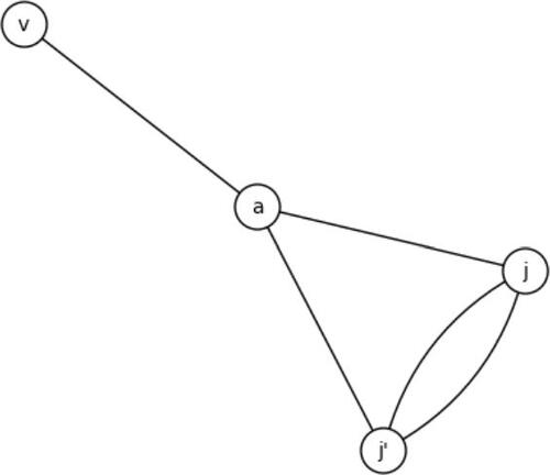
Let v_a be the unique surface vertex of V (see Figure 7). This gives us two distinct loops in ${\mathcal{G}}_2({\overline{\mathbb{F}}}_p)$ of length 3 corresponding to endomorphisms of norm 8 in ${\text{End}}_{{\overline{\mathbb{F}}}_p}(E_{\mathbf{j}})$.

Fig. 7 The double edge from j to $\mathbf{j}\prime$.

To check for the existence of such an endomorphism, we need to check whether the roots of f(X) can simultaneously be the roots of the modular polynomial ${\Phi }_8(X,X)$. Taking the resultant $\mathrm{Res}(f(X),{\Phi }_8(X,X))$ we get$$(-1)·3^{72}·5^{36}·7^{48}·{11}^{34}·{13}^{24}·{37}^{10}·{41}^2·{43}^8·{59}^2·71·{89}^2·{101}^2.$$

For primes p > 101, this will be nonzero, and there is no such a loop in ${\mathcal{G}}_2({\overline{\mathbb{F}}}_p)$; hence, attachment happens. In the factorization of the resultant, there are two primes satisfying $p\equiv 11,59\text{mod}60$ and $3\text{mod}8$. For p = 11, we only have one connected component of ${\mathcal{G}}_2({\mathbb{F}}_p)$, for p = 59, attachment happens. □

In the case $p\equiv 7\text{mod}8$, not all attachments that can happen necessarily do. We checked this for all primes $p\equiv 7\text{mod}8$ between 50, 000 and 100, 000 such that the primes above 2 do not generate the class group (in this case, there is clearly only one connected component of $\mathcal{S}$). There are 217 such primes, and for 41 of them the attachment happens. However, there are 12 primes p for which the attachment can happen ($p\equiv 11$ or 59 $\text{mod}60$) but there is no attachment. For instance, for p = 53639, the two roots of f(X) are $\mathbf{j}=30505$ and $\mathbf{j}=46665$. There are two elliptic curves with these j-invariants on the same component of ${\mathcal{G}}_2({\mathbb{F}}_p)$ which are 48 edges apart.

3.5 Distances between the components of the $\mathcal{S}\subset {\mathcal{G}}_2({\mathbb{F}}_p)$

In Sections 3.3 and 3.4, we described how the spine $\mathcal{S}$ is formed by passing from ${\mathcal{G}}_{\mathcal{l}}({\mathbb{F}}_p)$ to ${\mathcal{G}}_{\mathcal{l}}({\overline{\mathbb{F}}}_p)$. In principle, one can then describe the shape and connectedness of $\mathcal{S}$ based on the knowledge of ${\mathcal{G}}_{\mathcal{l}}({\overline{\mathbb{F}}}_p)$ and congruence conditions on p. A natural and important question is how the spine $\mathcal{S}$ sits inside the graph ${\mathcal{G}}_{\mathcal{l}}({\overline{\mathbb{F}}}_p)$. We study this question for $\mathcal{l}=2$.

For primes $p\equiv 1\text{mod}4$, the subgraph is given by single edges (with a possibility of an isolated vertex and one component of size 4), as we showed in Section 3.2. We expect the distances between components of the graph to behave like the distances between random vertices of the graph. 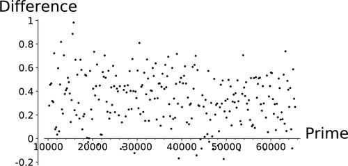To investigate if the ${\mathbb{F}}_p$-components are somehow distinguished, we compare the distances between ${\mathbb{F}}_p$-components with the distances between random vertices of the graph: In Figure 8, we compare these distances for 254 primes with $p\equiv 1\text{mod}4$ from 10253 to 65437. The primes were chosen to be spaced with a gap of at least 200. To approximate the distance between random points, we sample the distances between 100 pairs of random points on the graph. The vertical axis of this figure represents the difference [(average distance of ${\mathbb{F}}_p$-components) – (average distance between 100 random pairs of points)]. For this range of primes, the average distances between ${\mathbb{F}}_p$-components ranged between 8.20 and 10.95. The average distances between pairs of randomly chosen vertices ranged between 7.82 and 10.85. Notice that these differences are mostly positive: The average distances between components is slightly larger than distance between two random points in ${\mathcal{G}}_2({\overline{\mathbb{F}}}_p)$ (around 3.6% larger).

Fig. 8 Comparing average distances between random vertices in ${\mathcal{G}}_2({\overline{\mathbb{F}}}_p)$ and between connected components of $\mathcal{S}\subset {\mathcal{G}}_2({\overline{\mathbb{F}}}_p)$. On the horizontal axis, we have primes $p\equiv 1\text{mod}4$. The height of each point represents (avg. distance between ${\mathbb{F}}_p$-components) - (avg. distance between 100 random points of ${\mathcal{G}}_2({\overline{\mathbb{F}}}_p)$).

We now consider the case where $p\equiv 7\text{mod}8$. In this case, the graph ${\mathcal{G}}_2({\mathbb{F}}_p)$ is a union of 2-level volcanoes, each with $h(-p)$ vertices on the surface and $h(-p)$ vertices on the floor. The size of the surface of any volcano is the order of the prime above 2 in the class group $\text{cl}({\mathcal{O}}_K)$. If a prime above 2 generates the class group, ${\mathcal{G}}_2({\mathbb{F}}_p)$ is connected and so is $\mathcal{S}$. The converse is not true, as it is possible for $\mathcal{S}$ to become connected via attaching. In this case, we again compare the distances between ${\mathbb{F}}_p$-components and the distances between random vertices. In the range $50000<p<100000$, there are 217 primes for which a prime ${\mathfrak{p}}_2$ above 2 does not generate the class group. For these 217 primes, we observed that for 12 primes, the spine $\mathcal{S}$ is nonetheless connected. For 57 of those primes, there were exactly two connected components. The distances between these connected components was less than or equal to 6.

Table 1 Size and shape of the spine, depending on primes modulo 8, the integer n denotes the order of any prime above 2 in $\text{cl}({\mathcal{O}}_K)$.

prime mod 8	shape of ${\mathcal{G}}_2({\mathbb{F}}_p)$	$\#\mathcal{S}$	$\approx \#(\mathcal{S}$-Components)
$1\text{mod}4$	edges	$\frac{1}{2}h(-4p)$	$\frac{1}{4}h(-4p)$
$3\text{mod}8$	claw	$2h(-p)$	$\frac{1}{4}·2h(-p)=\frac{1}{2}h(-p)$
$7\text{mod}8$	volcanoes	$h(-p)$	$\frac{1}{2n}·h(-p)$

Note: The first dataset contains around 100 primes in each congruence class, the latter between 10 and 17 primes.

The graphs have between 5400 and 8300 vertices and diameters of length between 14 and 16. For 2-isogeny graphs of this size, the average distance between two random vertices is around 9 ($\sim 0.6\times$ diameter). This number grows slowly (for primes $p\approx 500000$, the average distance between two random vertices is $\sim 0.7\times$ diameter) and we expect it to converge to the diameter. We also computed the average of the mean distances between connected components of $\mathcal{S}\subset {\mathcal{G}}_2({\mathbb{F}}_p)$ for these primes. The mean is 4.3395, with standard deviation 1.1092. The maximum is 7.000 and the minimum 2.333, which indicates that the components tend to be close to each other.

3.6 The number of components in the spine for $\mathcal{l}=2$

In this section, we briefly comment on the number of connected components of $\mathcal{S}$ and relatedly, on the number of connected components in ${\mathcal{G}}_2({\mathbb{F}}_p)$. By Theorem 3.29, we know at most one component of $\mathcal{S}$ folds, and at most two components are attached by a new edge. It is therefore easy to determine the approximate number of components depending on the size of the spine and the shape of the connected components in ${\mathcal{G}}_2({\mathbb{F}}_p)$.

The number of vertices in $\mathcal{S}$ can be determined from [9]$$\#\mathcal{S}=\{\begin{array}{cc}\frac{1}{2}h(-4p)\hfill & \mathrm{}\text{if}\mathrm{}p\equiv 1\text{mod}4,\hfill \\ h(-p)\hfill & \mathrm{}\text{if}\mathrm{}p\equiv 7\text{mod}8,\hfill \\ 2h(-p)\hfill & \mathrm{}\text{if}\mathrm{}p\equiv 3\text{mod}8.\hfill \end{array}$$where h(d) is the class number of the imaginary quadratic field $\mathbb{Q}\left(\sqrt{d}\right)$. Using standard estimates for class numbers, one typically approximates $h(d)\approx \sqrt{\left|d\right|}$.

4 Conjugate vertices, distances, and the spine

The existence of mirror paths (see Definition 2.6) in ${\mathcal{G}}_{\mathcal{l}}({\overline{\mathbb{F}}}_p)$ motivates us to question their length in relation to the diameter of the graph. Delfs and Galbraith [11] show that if one navigates to the spine $\mathcal{S}$, one can solve the path finding problem in subexponential time using the quantum algorithm in [3]. This leads naturally to the question of how the spine $\mathcal{S}$ sits in the full $\mathcal{l}$-isogeny graph. We consider these questions from three perspectives in this chapter. In Section 4.1 we study the distance between Galois conjugate pairs of vertices, that is, pairs of $\mathit{j}$-invariants of the form $\mathit{j}$, ${\mathit{j}}^p$. Our data suggest these vertices are closer to each other than a random pair of vertices in ${\mathcal{G}}_2({\overline{\mathbb{F}}}_p)$. In Section 4.2, we test how often the shortest path between two conjugate vertices goes through the spine $\mathcal{S}$ (contains a j-invariant in ${\mathbb{F}}_p$). We find conjugate vertices are more likely than a random pair of vertices to be connected by a shortest path through the spine. Finally, we continue to examine the question of navigating to the spine $\mathcal{S}$ by considering the distance between arbitrary vertices and the spine $\mathcal{S}$ in Section 4.3.

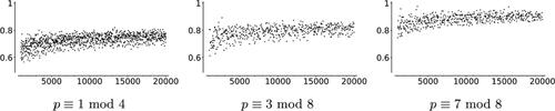
4.1 Distance between conjugate pairs

Isogeny-based cryptosystems such as cryptographic hash functions and key exchange algorithms rely on the difficulty of computing paths (routing) in the supersingular graph ${\mathcal{G}}_{\mathcal{l}}({\overline{\mathbb{F}}}_p)$. Our experiments with $\mathcal{l}=2$ show that two random conjugate vertices are closer than two random vertices. These shorter distances may indicate that it is computationally easier to find paths between conjugate vertices, when compared with random graph vertices. We analyze the differences between these distances in this section, using the following experimental practices: Given prime p, we constructed the graph ${\mathcal{G}}_2({\overline{\mathbb{F}}}_p)$. Then we computed the distances $\text{dist}({\mathit{j}}_1,{\mathit{j}}_2)$ between all pairs of $({\mathbb{F}}_{p^2}\setminus {\mathbb{F}}_p)$-vertices ${\mathit{j}}_1,{\mathit{j}}_2\in {\mathcal{G}}_2({\overline{\mathbb{F}}}_p)$. These values were organized into two lists: $$\begin{array}{c}{C}_p=[\text{dist}(\mathit{j},{\mathit{j}}^p):\mathit{j}\in {\mathbb{F}}_{p^2}\setminus {\mathbb{F}}_p],\\ A_p=[\text{dist}({\mathit{j}}_1,{\mathit{j}}_2):{\mathit{j}}_1,{\mathit{j}}_2\in {\mathbb{F}}_{p^2}\setminus {\mathbb{F}}_p].\end{array}$$

We call the pairs from C_p conjugate pairs and pairs from A_p arbitrary pairs.

The distributions C_p and A_p for p = 19489 are shown in Figure 9. For a larger prime, it is too costly to iterate over all vertices. Instead, we took a random sample of 1000 conjugate and arbitrary pairs. The data collected for the prime p = 1000003 is shown in Figure 10.

Fig. 9 Histogram of distances measured between conjugate pairs and arbitrary pairs of vertices not in ${\mathbb{F}}_p$ for the prime $p=19,489$.

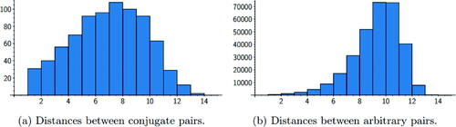
Fig. 10 Histogram of distances between 1000 randomly sampled pairs of arbitrary and conjugate vertices for the prime $p=1,000,003$.

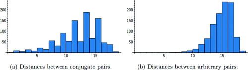
In these examples, we see different distributions for the conjugate pair distances compared with the arbitrary pair distances. For both primes, conjugate pairs are more likely to be closer than arbitrary pairs. This indicates that conjugate pairs of vertices have a somehow special position in the graph. This is likely related to the fact that the neighbors of curves with conjugate j-invariants are also conjugate, as discussed in Section 2.

In Figure 10, we see a clear bias toward paths of odd length (that is, paths with an odd number of edges). This is due to the fact that conjugate j-invariants often admit a shortest path that is a mirror path (Definition 2.6). These paths do not usually go through the spine $\mathcal{S}$, so they have an even number of vertices and an odd number of edges. This topic is studied further in Section 4.2.

Further studies on a broader sample of primes would be required to fully explore the differences between the distributions of distances between conjugate and arbitrary vertices.

4.2 How often do shortest paths go through the spine $\mathcal{S}$

Motivated by the work of Delfs and Galbraith [11], we consider the question of how easy it is to navigate to the spine $\mathcal{S}$. In their work, Delfs–Galbraith use L-isogenies to navigate to the spine $\mathcal{S}$, where L is a set of small primes. We study the situation when $L=\left\{2\right\}$. Any path from $\mathit{j}$ to a vertex j in the spine $\mathcal{S}$ can then be mirrored to obtain a path of equal length from j to ${\mathit{j}}^p$, and hence a path between $\mathit{j}$ and ${\mathit{j}}^p$ passing through the spine. This construction motivates the following definition:

Definition 4.1.

A pair of vertices are opposite if there exists the shortest path between them that passes through the ${\mathbb{F}}_p$ spine.

4.2.1 Experimental methods

We used built-in functions of Sage [26] to perform our computations. We tested how often a shortest path between two conjugate vertices went through the spine $\mathcal{S}$. Shortest paths are not necessarily unique, so it is not enough to compute a shortest path and check whether it passes through the spine. Instead, to verify whether a pair ${\mathit{j}}_1,{\mathit{j}}_2$ is opposite, we run over all vertices in $\mathbf{j}\in {\mathbb{F}}_p$ and check whether there is a j such that$$\mathit{dist}({\mathit{j}}_1,{\mathit{j}}_2)=\mathit{dist}({\mathit{j}}_1,\mathbf{j})+\mathit{dist}(\mathbf{j},{\mathit{j}}_2).$$

For smaller primes (< 5000), we computed the proportions for all pairs of vertices in ${\mathbb{F}}_{p^2}\backslash {\mathbb{F}}_p$. For larger primes, we randomly selected 1000 pairs of points ${\mathit{j}}_1,{\mathit{j}}_2$ in ${\mathbb{F}}_{p^2}\backslash {\mathbb{F}}_p$ and checked whether each of the pairs $({\mathit{j}}_1,{\mathit{j}}_2),({\mathit{j}}_1,{\mathit{j}}_1^p)$ were opposite.

In the following two subsections, we present these data sorted in two ways: comparing conjugate pairs and arbitrary pairs, and comparing differences in distances between arbitrary vertices for different congruence classes of $p\text{mod}8$.

4.2.2 Conjugate pairs vs. arbitrary pairs

For each prime p ranging between 50000 and 100000, we sampled data from 1000 random conjugate pairs of vertices and 1000 pairs of arbitrary vertices. We computed the proportions of conjugate pairs which are opposite and the proportions of arbitrary pairs which are opposite. This data is displayed in Figure 11.

Fig. 11 Proportions of vertex pairs that are opposite; x-axis represents primes. The data are for a random sample of 1000 pairs of conjugate and arbitrary pairs.

Our data suggest conjugate vertices are more likely to be opposite than arbitrary vertices and that this bias increases with p. For the primes displayed in Figure 11, conjugate pairs are more than four times as likely to be opposite, compared with arbitrary pairs. For $1000<p<5000$ (not displayed), conjugate pairs are approximately twice as likely to be opposite than random pairs.

The graph ${\mathcal{G}}_{\mathcal{l}}({\overline{\mathbb{F}}}_p)$ can be symmetrically constructed from $\mathcal{S}$ by adding edges and mirror edges at once, leading one to suspect $\mathcal{S}$ to be central to the graph. However, we have found the shortest paths between arbitrary pairs of vertices are less likely to pass through the spine, contradicting that perspective.

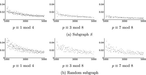
4.2.3 Varying the residue class of p

In this section, we consider only arbitrary pairs of vertices, and we study the overall connectivity of the graph by looking at the proportions of opposite arbitrary vertices, for primes p in different congruence classes modulo 8. See Figure 12.

Fig. 12 The horizontal axes of these figures are primes. The heights are proportions of 1000 pairs of arbitrary vertices which are opposite, normalized by $\left|\mathcal{S}\right|$.

In these data, we have computed for each prime p a random sample of 1000 arbitrary pairs of vertices and checked how many are opposite. Then, we take this number and divide by $1000·\left|\mathcal{S}\right|$, to account for differences in the numbers of ${\mathbb{F}}_p$ vertices for these primes. We have sorted the data by primes $p\text{mod}8$ and displayed it in the graphs in Figure 12. Our results suggest that the size and connectedness of the spine $\mathcal{S}$ could be the key factor affecting the proportion of opposite pairs:

1. Size of $\mathcal{S}$: Shortest paths are more likely to pass through $\mathcal{S}$ if it is larger. We account for this by dividing the proportions of opposite arbitrary pairs of vertices by $\left|\mathcal{S}\right|$ in Figure 12. The normalized proportions still differ modulo 8, indicating another factor is at play, possibly the connectedness of $\mathcal{S}$.

2. Connectedness of $\mathcal{S}$: When $\mathcal{S}$ is less connected, pairs are more likely to have shortest paths through it. From the table in Section 3.6, the spine is the least connected when $p\equiv 1\text{mod}4$, and can be most connected when $p\equiv 7\text{mod}8$. This could explain the difference in proportions when normalized by the size of $\mathcal{S}$.

   For example, consider $p_1=19991$ ($p_1\equiv 7\text{mod}8,\mathcal{S}$ is connected, $\left|\mathcal{S}\right|=199$) and $p_2=19993$ ($p\equiv 1\text{mod}4,\mathcal{S}$ is maximally disconnected, $\left|\mathcal{S}\right|=30$). We would expect $199/30>6$ times more opposite pairs in the p₁ case. However, for 1000 arbitrary pairs, only 266 pairs were opposite for p₁ compared to 112 pairs for p₂.

To further study whether differences occurring in the normalized proportions of vertices which are opposite for $p\text{mod}8$ were due to the connectedness of $\mathcal{S}$, we took a random subgraph of the same size as $\mathcal{S}$ and obtained the proportion of pairs of arbitrary vertices with a shortest path passing through the random subgraph. We took the average of these results over 10 random subgraphs for each prime between 1000 and 5000. The data, in Figure 13, show less distinction $\text{mod}8$ compared to the data in Figure 12. This suggests that the connectedness of $\mathcal{S}$ is a dominant factor affecting the normalized proportion of opposite pairs of vertices.

Fig. 13 Normalized proportion of pairs with a shortest path through the specified subgraph, as p varies.

4.3 Distance to spine

In this section, we investigate how connected the spine is to the rest of the graph, motivated by the path-finding algorithm of Delfs and Galbraith [11].

4.3.1 Distance to the spine versus a random subgraph

For two fixed primes, we study how the spine fits into the graph, and compare this with a randomly selected subgraph. Specifically, we compare a random vertex’s distance to the spine, with a random vertex’s distance to a random subgraph of the same size as the spine. We observe that if the spine is connected, then the distance to the spine seems greater than the distance to a random subgraph. This agrees with the intuition that a small connected subgraph ($\left|\mathcal{S}\right|\approx O\left(\sqrt{p}\right)$) will be further from most vertices than a random subgraph, which will have many connected components uniformly distributed throughout the graph.

We studied these distances for the primes, p = 19991 and $p=19993$. For p = 19991, the subgraph $\mathcal{S}$ is connected, and for p = 19993, $\mathcal{S}$ is maximally disconnected (see [11]). For each value of p, we constructed the graph ${\mathcal{G}}_2({\overline{\mathbb{F}}}_p)$, the spine $S_0:=\mathcal{S}$, and chose several random subgraphs $S_1,\dots ,S_n$. We define the distance between a vertex j and a subgraph S_i to be$$\text{dist}(j,S_i)=\min \{\text{dist}(j,j\prime ):j\prime \in S_i\}.$$

We computed lists $d_i=[\text{dist}(j,S_i):j\in {\mathcal{G}}_2({\overline{\mathbb{F}}}_p)]$ in order to measure how dispersed S_i is in ${\mathcal{G}}_2({\overline{\mathbb{F}}}_p)$. Histograms of the distributions of the d_i are given in Figure 14.

Fig. 14 Distances to the spine $\mathcal{S}$ contrasted with distances to a random subgraph R of the same size. The spine $\mathcal{S}$ is connected for p = 19, 991 and a union of disconnected edges for p = 19, 993.

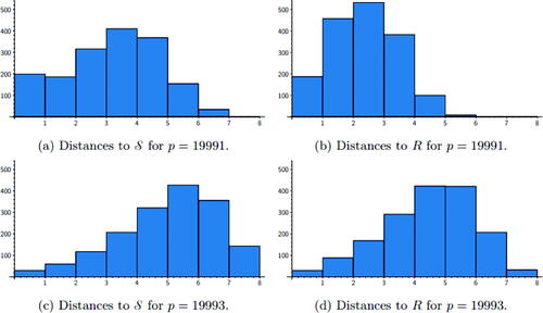
The significant difference between the two primes shown in Figure 14 can also be explained by the number of vertices in $\mathcal{S}$. Since ${\mathcal{G}}_2({\overline{\mathbb{F}}}_p)$ is a 3-regular graph, for a random vertex j, there are at most $3·2^{d-1}$ vertices of distance d away from j (and this limit is achieved if there are no collisions on the paths leaving j). If ${\mathcal{G}}_2({\overline{\mathbb{F}}}_p)$ has N vertices and H is a random subgraph with M vertices, then the expected distance to H from a random vertex should be $\approx {\hspace{0.17em}\text{log}\hspace{0.17em}}_2(N/M)$. For p = 19991, $\left|\mathcal{S}\right|=199$, so we expect the average distance to $\mathcal{S}$ to be 3.06. For p = 19993, $\left|\mathcal{S}\right|=30$, so we expect the average distance to $\mathcal{S}$ to be 5.80.

When maximally disconnected, the distances to the spine were similar to that of a random subgraph. However, when the spine is connected, the distances are slightly longer. This shows that modeling the spine as a random subgraph may lead to an underestimate of the distances.

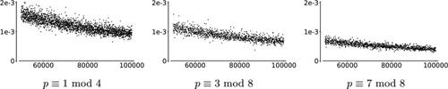
4.3.2 Comparison across primes p

In order to compare the distances to $\mathcal{S}$ across different primes and account for the expected average distance based on the size of $\mathcal{S}$ we consider normalized distances as follows:$$d_p=(\text{average}\mathrm{}\text{distance}\mathrm{}\text{to}\mathrm{}\mathcal{S}\mathrm{}\text{for}\mathrm{}\text{prime}\mathrm{}p)/{\hspace{0.17em}\text{log}\hspace{0.17em}}_2(|{\mathcal{G}}_2({\overline{\mathbb{F}}}_p)|/|\mathcal{S}|).$$

Recall that ${\hspace{0.17em}\text{log}\hspace{0.17em}}_2(|{\mathcal{G}}_2({\overline{\mathbb{F}}}_p)|/|\mathcal{S}|)$ is the expected distance to the spine from a random vertex. We observed that the average distances were lower than the expected distance based on the connectedness of $\mathcal{S}$. There are also clear differences in the distributions of d_p when considering residue classes of p modulo 8. This is shown in Figure 15. In particular, the data $\text{mod}8$ match our findings on the proportion of opposite pairs, see Figure 12.

Fig. 15 Normalized average distances d_p to the spine $\mathcal{S}$, as prime p varies on the horizontal axes.

However, the different behavior of d_p for the different congruence classes $\text{mod}8$ can be explained by the size of the spine. If the size of the spine $\left|\mathcal{S}\right|$ is large, we will need fewer steps to reach the spine from a random vertex v. Hence, when counting the paths of length d from v, we will encounter less backtracking and the estimate is more precise. Looking at Figure 16, we see that for $p\equiv 7\text{mod}8$, the size of the spine is the largest, and for $p\equiv 1\text{mod}4$, the size of the spine is the smallest.

Fig. 16 Size of the spine as prime p varies on the horizontal axes.

We also tested this within a fixed congruence class: for primes p with $p\equiv 7\text{mod}8$ and $15000<p<20000$, the mean distance to the spine is 4.040 with standard deviation 0.413 if $\left|\mathcal{S}\right|<100$ and mean 3.007 with standard deviation 0.335 if $\left|\mathcal{S}\right|>100$.

5 When are conjugate j-invariants $\mathcal{l}$-isogenous?

5.1 Motivation

In Section 4.2, we studied paths between conjugate j-invariants in ${\mathcal{G}}_2({\overline{\mathbb{F}}}_p)$ that go through the spine $\mathcal{S}$. If $\mathit{j}$ and ${\mathit{j}}^p$ happen to be 2-isogenous, then the shortest path between them has length one and does not go through $\mathcal{S}$. This leads us to the natural question:

Question 1. How often are conjugate ${\mathbb{F}}_{p^2}\setminus {\mathbb{F}}_p$ j-invariants $\mathcal{l}$-isogenous, for $\mathcal{l}=2,3$?

5.2 Experimental data: 2-isogenies

We collected data on supersingular j-invariants over ${\mathbb{F}}_{p^2}$ for all primes $5\le p\le 100193$ (a total of 9605 primes). For each p, we determined all of the ${\mathbb{F}}_{p^2}\setminus {\mathbb{F}}_p$ j-invariants and counted those that are also 2-isogenous to their conjugates.

With a few exceptions, all of the proportions computed are positive and strictly less than 1. The small primes (roughly p < 5000) have a wide range of proportions, between 0 and 1. This is expected due to the small number of points on their ${\mathcal{G}}_{\mathcal{l}}({\overline{\mathbb{F}}}_p)$ graphs. For example: there are some primes p such that all of the pairs of conjugates are 2-isogenous. On the other hand, if ${\mathcal{G}}_{\mathcal{l}}({\overline{\mathbb{F}}}_p)\setminus {\mathcal{G}}_{\mathcal{l}}({\mathbb{F}}_p)=\varnothing$ then the proportion will be trivially zero. This happens only for 15 small primes, namely those dividing the order of the Monster group [21]. Notably, the only examples of p for which the proportion is zero, but not trivially zero, are p = 101, 131.

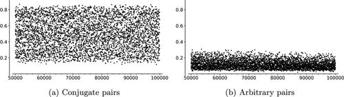
To avoid small prime phenomena, we focused on analyzing the data we collected for $10007\le p\le 100,193$, a total of 8378 primes. The graph of proportions for these data can be found in Figure 17. We found that the mean proportion in the data is 0.032780 with a standard deviation of 0.019134.

Fig. 17 Proportion of 2-isogenous conjugate pairs in ${\mathcal{G}}_2({\overline{\mathbb{F}}}_p)$ for $10,007\le p\le 100,193.$

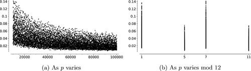
We then sorted the data by congruence conditions to look for patterns. The biggest difference appeared when we re-sorted the data according to the congruence class of the primes modulo 12. The primes in this range are fairly evenly distributed into the congruence classes modulo 12, as one can see in Table 2.

Table 2 Proportions of 2-isogenous conjugates, $10007\le p\le 100193$, sorted by $p\text{mod}12$.

	$p\equiv 1\text{mod}12$	$p\equiv 5\text{mod}12$
Total # of primes:	2079	2104
Mean:	0.043551	0.021969
Standard deviation:	0.019815	0.010206
	$p\equiv 7\text{mod}12$	$p\equiv 11\text{mod}12$
Total # of primes:	2101	2094
Mean:	0.043375	0.022244
Standard deviation:	0.020140	0.010512

5.2.1 Primes modulo 12

In Table 2, we summarize the differences between the congruence classes modulo 12. Note the similar, higher means for $p\equiv 1,7\text{mod}12$ and the similar, lower means for $p\equiv 5,11\text{mod}12$. These distributions are skewed according to the congruence class, as we can also see from the graph in Figure 17(b). There appears to be a correlation between primes $p\equiv 1,7\text{mod}12$ and between primes $p\equiv 5,11\text{mod}12$. A two-sample t-test confirms these correlations at the 99.8% level.

5.3 Experimental data: 3-isogenies

We collected data on the supersingular j-invariants over ${\mathbb{F}}_{p^2}$ for all the primes $5\le p\le 100193$ (a total of 9,605 primes) and computed the proportion of conjugate pairs that are also 3-isogenous. We present these data in the same format as the 2-isogeny data presented in Section 5.2.

Once again, we observe some small prime phenomena (proportions of 1 and 0 for p small). However, in the 3-isogeny case we do not have nontrivial examples of primes p for which the proportion of 3-isogenous conjugates is 0. On the contrary, if there exist conjugate j-invariants in ${\mathbb{F}}_{p^2}\setminus {\mathbb{F}}_p$, then there is at least one pair of 3-isogenous conjugates. (Recall that the two counterexamples to this statement in the 2-isogeny case were p = 101131.)

To avoid small prime phenomena, we again focused on analyzing the data we collected for $10007\le p\le 100193$, a total of 8378 primes. The graph of proportions for these data can be found in Figure 18.

Fig. 18 Proportion of 3-isogenous conjugate pairs in ${\mathcal{G}}_2({\overline{\mathbb{F}}}_p)$ for $10,007\le p\le 10,0193.$

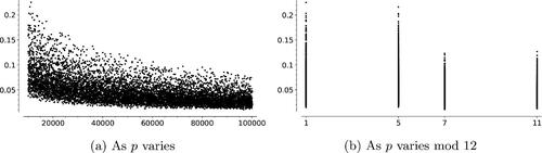
In this collection of data, for primes $10007\le p\le 100193$, we found there to be a mean proportion of 3-isogenous conjugate pairs of 0.047306, with standard deviation of 0.026568.

As in the 2-isogeny case, we again sorted the data by congruence conditions to look for patterns. The biggest difference appeared when we re-sorted the data according to the congruence class of the primes modulo 12.

5.3.1 Primes modulo 12

In Table 3, we summarize the differences between the different congruence classes modulo 12. Note the similar and higher means for $p\equiv 1,5\text{mod}12$ and the similar and lower means for $p\equiv 7,11\text{mod}12$, as we can also observe in Figure 18(b). There appears to be a correlation between primes $p\equiv 1,5\text{mod}12$ and between primes $p\equiv 7,11\text{mod}12$. A two-sample t-test confirms these correlations at the 99.8% level.

Table 3 Proportions of 3-isogenous conjugates for $10007\le p\le 100193$, sorted by $p\text{mod}12.$

	$p\equiv 1\text{mod}12$	$p\equiv 5\text{mod}12$
Total # of primes:	2079	2104
Mean:	0.058526	0.059034
Standard deviation:	0.029488	0.029729
	$p\equiv 7\text{mod}12$	$p\equiv 11\text{mod}12$
Total # of primes:	2101	2094
Mean:	0.035620	0.036107
Standard deviation:	0.016369	0.016706

5.4 Further Questions

Our experimental data suggest that, at least for $\mathcal{l}=2,3$ and with the exception of a few small primes, the proportion of conjugate pairs that are $\mathcal{l}$-isogenous is a small positive number. In particular, all of the primes $p\ne 101,131$ with supersingular j-invariants in ${\mathbb{F}}_{p^2}\setminus {\mathbb{F}}_p$ observed have at least one such pair. This motivates the following two questions:

Question 2. For p > 131, is there always at least one pair of $\mathcal{l}$-isogenous conjugate j-invariants on ${\mathcal{G}}_{\mathcal{l}}({\overline{\mathbb{F}}}_p)$?

Question 3. For large p, is there a nontrivial lower and/or upper bound for the proportion of $\mathcal{l}$-isogenous conjugate j-invariants on ${\mathcal{G}}_{\mathcal{l}}({\overline{\mathbb{F}}}_p)$?

A partial answer to Question 3 can be found in Lemma 6 of [6], which states that, in the case when $p\equiv 1\text{mod}12$, the set of j-invariants that are adjacent to their conjugates in ${\mathcal{G}}_{\mathcal{l}}({\overline{\mathbb{F}}}_p)$ is of size $\sqrt{\mathcal{l}}\tilde{O}\left(\sqrt{p}\right)$, which yields an upper bound. [14] provided an answer regarding the lower bound in Question 3, and thus also for Question 2. [14] is concerned with computing endomorphism rings of supersingular elliptic curves over ${\mathbf{F}}_{p^2}$ by finding cycles in ${\mathcal{G}}_2({\overline{\mathbb{F}}}_p)$. The construction of these cycles involves finding j-invariants that are adjacent to their ${\mathbb{F}}_p$-conjugates. As part of the analysis of the algorithm, they proved that the cardinality of the set of such j-invariants is larger than $C\frac{\sqrt{p}}{\hspace{0.17em}\text{log}\hspace{0.17em}\hspace{0.17em}\text{log}\hspace{0.17em}p}$, for some constant C depending on $\mathcal{l}$ (assuming GRH). Both of these proofs assume that $\mathcal{l}<p/4$.

However, these bounds do not seem to explain the significant difference in the average of the proportion of $\mathcal{l}$-isogenous conjugate pairs when we vary the congruence class of p modulo 12. This prompts us to formulate the question:

Question 4. How does the proportion of $\mathcal{l}$-isogenous conjugate j-invariants on ${\mathcal{G}}_{\mathcal{l}}({\overline{\mathbb{F}}}_p)$ relate to the conjugacy class of $p\text{mod}12$?

Remark 5.1.

We can also consider $\mathcal{l}$-isogenous conjugate pairs of j-invariants in the context of the modular curve $X_0(\mathcal{l})$. In [21], Ogg defined $X_0{(\mathcal{l})}^{+}$, the Atkin-Lehner quotient of $X_0(\mathcal{l})$ by the Fricke involution. If two conjugate ${\mathbb{F}}_{p^2}\setminus {\mathbb{F}}_p$ j-invariants $\mathit{j},{\mathit{j}}^p$ are $\mathcal{l}$-isogenous, then $(\mathit{j},{\mathit{j}}^p)$ is a point of $X_0(\mathcal{l})$. The image of $(\mathit{j},{\mathit{j}}^p)$ under the quotient map is an ${\mathbb{F}}_p$-rational point of $X_0{(\mathcal{l})}^{+}$. Conversely, any ${\mathbb{F}}_p$-rational point of $X_0{(\mathcal{l})}^{+}$ whose preimage in $X_0(\mathcal{l})$ contains a non-${\mathbb{F}}_p$ point corresponds to an $\mathcal{l}$-isogenous conjugate pair $\mathit{j},{\mathit{j}}^{\mathrm{p}}$. Intersecting with the supersingular locus, we have an alternative description of the set of ${\mathbb{F}}_{p^2}\setminus {\mathbb{F}}_p$ $\mathcal{l}$-isogenous conjugate pairs in the Supersingular Isogeny Graph.

6 Diameter

Numerical experiments in [22] estimated the diameters of k-regular LPS Ramanujan graphs and random Cayley graphs to be asymptotically $\frac{4}{3}·{\hspace{0.17em}\text{log}\hspace{0.17em}}_{k-1}(n)$ and ${\hspace{0.17em}\text{log}\hspace{0.17em}}_{k-1}(n)$ respectively, where n is the number of vertices. We present data on the diameters of the supersingular 2-isogeny graphs, which are 3-regular on $p/12+ϵ$ vertices, with $ϵ=0,1$, or 2, depending on the congruence class of p $\text{mod}12$.

For $p\equiv 3\text{mod}4$, the j-invariant 1728 appears in a special place of the graph - it is only 2-isogenous to one other curve. This isolated position in the graph may lead to longer diameters of ${\mathcal{G}}_{\mathcal{l}}({\overline{\mathbb{F}}}_p)$ for $p\equiv 3\text{mod}4$.

We can see a lower bound$${\hspace{0.17em}\text{log}\hspace{0.17em}}_2\left(\lfloor \frac{p}{12}\rfloor \right)-{\hspace{0.17em}\text{log}\hspace{0.17em}}_2(3)+1$$on the diameter as follows. Starting from a random vertex and taking a walk of length n, the walk reaches at most $3·2^{n-1}$ vertices as endpoints (exactly that number if there are no collisions). Since there are $\lfloor \frac{p}{12}\rfloor +ϵ$ vertices in the graph, with $ϵ=0,1,2$, the diameter cannot be less that the smallest n₀ such that$$3·2^{n_0-1}+1\ge \lfloor \frac{p}{12}\rfloor +ϵ.$$

We collected graph data for the diameters of the supersingular 2-isogeny graphs ${\mathcal{G}}_2({\overline{\mathbb{F}}}_p)$ for 4600 primes p. We used the built-in Sage” diameter” function [26] on the graphs. The implementation can be found in the walk.sage worksheet available on our github repository. We collected diameters of ${\mathcal{G}}_2({\overline{\mathbb{F}}}_p)$ in batches for ranges of primes. The smallest prime we have data for is $p=1009$ and the largest is p = 9501511. This data is displayed in Figure 19.

Fig. 19 Diameter of ${\mathcal{G}}_2({\overline{\mathbb{F}}}_p)$ for 4600 primes p with $1009\le p\le 9,501,511$ with $y={\hspace{0.17em}\text{log}\hspace{0.17em}}_2(p/12)+1+{\hspace{0.17em}\text{log}\hspace{0.17em}}_2(12)$ (dashed), $y=4/3{\hspace{0.17em}\text{log}\hspace{0.17em}}_2(p/12)+1$ (solid) and the proven lower bound $y={\hspace{0.17em}\text{log}\hspace{0.17em}}_2(p/12)-{\hspace{0.17em}\text{log}\hspace{0.17em}}_2(3)+1$ (dotted).

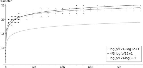
The shifted $(4/3){\hspace{0.17em}\text{log}\hspace{0.17em}}_2(p/12)$ graph (in a solid line) seems to increase too steeply for larger prime values. This could suggest that the 2-isogeny graph diameters may be more like random Cayley graphs, i.e. with distribution closer to ${\hspace{0.17em}\text{log}\hspace{0.17em}}_2(p/12)$. However, our numerical data are inconclusive: diameters for larger primes would be needed to make a conclusion, but our algorithm would not be able to find those in a reasonable amount of time.

For this reason, we adjusted our algorithm to find lower bounds on the diameter: We chose $\mathbf{j}=0$ as the starting vertex and in every step, we added the neighbors of all the known vertices, and truncated the computation instead of computing the entire graph. This gives a lower bound on the diameter. This algorithm allowed us to find lower bounds for the diameters of ${\mathcal{G}}_{\mathcal{l}}({\overline{\mathbb{F}}}_p)$ for larger primes p, shown in Figure 20. We see in Figure 20(b) that the dashed curve $y={\hspace{0.17em}\text{log}\hspace{0.17em}}_2(p/12)+{\hspace{0.17em}\text{log}\hspace{0.17em}}_2(12)+1$ no longer fits the data. We chose primes $p\equiv 23\text{mod}24$. See Section 6.1 for discussion on the difference $\text{mod}12$; we also chose $p\equiv 7\text{mod}8$ so that the spine $\mathcal{S}$ (see Definition 2.5) has the same structure and approximate size (see Section 3.6).

Fig. 20 Lower bounds on the diameter of ${\mathcal{G}}_2({\overline{\mathbb{F}}}_p)$ for 431 primes $p\equiv 23\text{mod}24$ with $1020431<p<15201671$, along with the graphs of $y={\hspace{0.17em}\text{log}\hspace{0.17em}}_2(p/12)+\alpha$ (dashed), $y=4/3{\hspace{0.17em}\text{log}\hspace{0.17em}}_2(p/12)+\beta$ (solid).

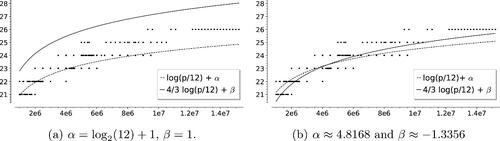
We tried fitting the curves ${\hspace{0.17em}\text{log}\hspace{0.17em}}_2(p/12)+\alpha$ and $4/3{\hspace{0.17em}\text{log}\hspace{0.17em}}_2(12)+\beta$ with the best constants α, β and as a first approximation we tried minimizing the sum of squares of distances to these curves, yielding $\alpha \approx 4.8168$ and $\beta \approx -1.3356$.

6.1 How does diameter vary for different congruence classes of primes modulo 12?

We investigated the behavior of the diameter as p varies modulo 12. We found a slight, but noticeable, bias: Primes $p\equiv 5,11\text{mod}12$ tend to have a 2-isogeny graph of larger diameter compared with primes $p\equiv 1,7\text{mod}12$. This is visible in Figures 21(a) and 21(b). In Figure 21(b), the diameters tend to be slightly larger than the graph of $y={\hspace{0.17em}\text{log}\hspace{0.17em}}_2(p/12)+{\hspace{0.17em}\text{log}\hspace{0.17em}}_2(12)+1$, whereas those in Figure 21(a) tend to be more evenly distributed above and below $y={\hspace{0.17em}\text{log}\hspace{0.17em}}_2(p/12)+{\hspace{0.17em}\text{log}\hspace{0.17em}}_2(12)+1$. Table 4 supports the visible bias.

Fig. 21 Diameters of 2-isogeny graph over ${\overline{\mathbb{F}}}_p$ for different congruence classes of the prime p, shown with $y={\hspace{0.17em}\text{log}\hspace{0.17em}}_2(p/12)+{\hspace{0.17em}\text{log}\hspace{0.17em}}_2(12)+1$

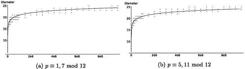
Table 4 Average diameters sorted by primes modulo 12.

average diameter for $100,000<p<300,000$
$1\text{mod}12$	17.2190476190476	$5\text{mod}12$	17.8761061946903
$7\text{mod}12$	17.7346938775510	$11\text{mod}12$	17.9919354838710
average diameter for $300,000<p<500,000$
$1\text{mod}12$	18.4000000000000	$5\text{mod}12$	18.9230769230769
$7\text{mod}12$	18.8235294117647	$11\text{mod}12$	19.1000000000000

7 Conclusions

We determined how the connected components of ${\mathcal{G}}_{\mathcal{l}}({\mathbb{F}}_p)$ merge together to give the spine $\mathcal{S}\subset {\mathcal{G}}_{\mathcal{l}}({\overline{\mathbb{F}}}_p)$. For any specific $\mathcal{l}$ and any p, one can determine the resulting shape explicitly if one knows the structure of the class group $\text{cl}({\mathcal{O}}_K)$.

For $\mathcal{l}=2$, we summarize the biases we observed in our heuristic data, for the different congruence classes of $p\text{mod}12$. The data suggest the following, although more careful analysis is needed to confirm:

• $p\equiv 1\text{mod}12$:

  • smaller 2-isogeny graph diameters,

  • larger number of spinal components, and

  • larger proportion of 2-isogenous conjugate pairs,

• $p\equiv 11\text{mod}12$:

  • larger 2-isogeny graph diameters,

  • smaller number of spinal components, and

  • smaller proportion of 2-isogenous conjugate pairs.

Netherlands Organisation for Scientific Research;

Acknowledgments

This article is the result of a collaboration started at Alice Silverberg’s 60th birthday conference on open questions in cryptography and number theory https://sites.google.com/site/silverberg2018/. We would like to thank Heidi Goodson for her significant contributions to this project. We are grateful to Microsoft Research for hosting the authors for a follow-up visit. We would like to thank Steven Galbraith, Shahed Sharif, and Katherine E. Stange for helpful conversations. We thank the reviewers for their thoughtful and helpful comments, leading to a many improvements in this article. Authors are listed in alphabetical order; see https://www.ams.org/profession/leaders/ culture/CultureStatement04.pdf.

Declaration of Interest

No potential conflict of interest was reported by the author(s).

Additional information

Funding

CCN was partially supported by Universidad de Costa Rica. TS was partially supported by Alfred P. Sloan Foundation grant number G-2014-13575. JS was partially supported by the Dutch Research Council (NWO) through Gravitation-grant Quantum Software Consortium - 024.003.037.

References

- Gora Adj, O. A., Menezes, A. On isogeny graphs of supersingular elliptic curves over finite fields. Finite Fields Their Appl., 55, 268–283.
- Arpin, S., Camacho-Navarro, C., Lauter, K., Lim, J., Nelson, K., Scholl, T., Sotáková, J. (2019). Adventures in supersingularland.
- Biasse, J.-F., Jao, D., and Sankar, A. (2014), A quantum algorithm for computing isogenies between supersingular elliptic curves. In Progress in cryptology—INDOCRYPT 2014, volume 8885 of Lecture Notes in Comput. Sci., Springer, Cham, pp. 428–442.
- Costache, A., Feigon, B., Lauter, K., Massierer, M., Pusks, A. Ramanujan graphs in cryptography. In: Jennifer, S. B., Folsom, A., Laln, M., Manes, M. Eds., Research Directions in Number Theory, Association for Women in Mathematics Series, Springer International Publishing, pp. 1–40.
- Charles, D., Goren, E., Lauter, K. (2006), Cryptographic hash functions from expander graphs. Cryptology ePrint Archive, Report 2006/021. Available at: https://eprint.iacr.org/2006/021.
- Charles, D., Goren, Ey., and Lauter, K. (2009), Families of Ramanujan graphs and quaternion algebras, In: Groups and symmetries, CRM Proc. Lecture Notes, Amer. Math. Soc., Vol. 47, pp. 53–80.
- Castryck, W., Lange, T., Martindale, C., Panny, L., and Renes, J. CSIDH: An efficient post-quantum commutative group action. In: Peyrin, T., Galbraith, S., Advances in Cryptology ASIACRYPT 2018, Lecture Notes in Computer Science, Springer International Publishing, pp. 395–427.
- Cox, D. (1989), Primes of the form x2 + ny2. New York: John Wiley and Sons, Inc.
- Castryck, W., Panny, L., and Vercauteren, F. (2020), Rational isogenies from irrational endomorphisms. In: Canteaut, A., Ishai, Y., Eds., Advances in Cryptology EUROCRYPT 2020, Lecture Notes in Computer Science, Springer International Publishing, pp. 523–548.
- Delfs, C., and Galbraith, S. D. (2016), Computing isogenies between supersingular elliptic curves over 𝔽p. Des. Codes Cryptog., 78: 425–440. Available at: https://arxiv.org/pdf/1310.7789.pdf.
- Hallgren, E.S., Lauter, K., Morrison, T., and Petit, C. (2018), Supersingular isogeny graphs and endomorphism rings: Reductions and solutions. In: Nielsen, J. B., Rijmen, V., Eds., Advances in Cryptology EUROCRYPT 2018, Lecture Notes in Computer Science, Springer International Publishing, pp. 329–368.
- Eisentrger, K., Hallgren, S., Leonardi, C., Morrison, T., Park, J. Computing endomorphism rings of supersingular elliptic curves and connections to path-finding in isogeny graphs. In Proceedings of the Fourteenth Algorithmic Number Theory Symposium, Vol. 4, Mathematical Sciences Publishers, pp. 215–232.
- Galbraith, S. D., Petit, C., Shani, B., and Ti, Y. B. (2016), On the security of supersingular isogeny cryptosystems. In: Cheon, J. H., Hee, J., Takagi, T., Eds., Advances in Cryptology ASIACRYPT 2016, Lecture Notes in Computer Science, Springer.
- Ibukiyama, T. (1982), On maximal orders of division quaternion algebras over the rational number field with certain optimal embeddings. Nagoya Math. J., 88: 181–195.
- Jao, D., De Feo, L. Towards quantum-resistant cryptosystems from supersingular elliptic curve isogenies. In: Yang, B-Y., Ed., Post-Quantum Cryptography, Lecture Notes in Computer Science, Springer, pp. 19–34.
- Kaneko, M. (1989), Supersingular j-invariants as singular moduli mod p. Osaka J. Math., 26, 12.
- Kohel, D., Lauter, K., Petit, C., and Tignol, J-P. (2014), On the quaternion ℓ-isogeny path problem. LMS J. Comput. Math., 17: 418–432.
- Kohel, D. (1996), Endomorphism rings of elliptic curves over finite fields. PhD thesis, Berkely: University of California.
- Love, J., Boneh, D. Supersingular curves with small noninteger endomorphisms. In: Proceedings of the Fourteenth Algorithmic Number Theory Symposium, Vol. 4, Mathematical Sciences Publishers, pp. 7–22.
- Lubotzky, A., Phillips, R. S., Sarnak, P. C. (1988), Ramanujan graphs. Combinatorica, 8: 261–277. doi:10.1007/BF02126799
- Ogg, A. P. (1975), Automorphismes de courbes modulaires. Séminaire Delange-Pisot-Poitou. Théorie des nombres, 16:1–8.
- Sardari, N. T. Diameter of Ramanujan graphs and random cayley graphs. 39: 427–446.
- Shor, P. W. (1999), Polynomial-time algorithms for prime factorization and discrete logarithms on a quantum computer. SIAM Rev., 41: 303–332.
- Silverman, J. H. (2009), The Arithmetic of Elliptic Curves, 2nd ed. New York: Springer-Verlag.
- Sutherlandm, A. V. (2013), Isogeny volcanoes. In: ANTS X—Proceedings of the Tenth Algorithmic Number Theory Symposium, volume 1 of Open Book Ser. Berkeley, CA: Math. Sci. Publ., pp. 507–530.
- The Sage Developers. (2019), SageMath, the Sage Mathematics Software System (Version 8.7). Available at: https://www.sagemath.org.
- Vlu, J. (1971), Isognies entre courbes elliptiques. Comptes Rendus de l’Acadmie des Sciences de Paris, 273: 238–241.